1. Introduction
In negative ion plasma sources, the design of the extraction system must consider a possibly large current density of electrons
 $j_{e}$
, which are co-extracted with the ions,
 $\text{H}^{-}$
for example. A transverse magnetic field is applied to reduce the ratio
 $R_{j}$
of
 $j_{e}$
and the ion current density
 $j_{\text{H}^{-}}$
so that collisional effects needs to be modelled before any
 $R_{j}$
optimization. While the complete physics is overwhelmingly complex and 3-D in space, here we present a 1-D kinetic model of electron transport which retains the main effects of the collisions and magnetic field accounted for by adequate integrals, calculated in detail from a kinetic equation with a simple collisional term.
Use of integrodifferential equations (Morse & Feshbach Reference Morse and Feshbach1953), even if less common than PDE (partial differential equation) and ODE (ordinary differential equation) in source modelling, is necessary when kinetic effects are projected to spatial coordinates, as indicated by a classic model (Tonks & Langmuir Reference Tonks and Langmuir1929), where electric field component
 $E_{z}$
and ion production and motion along
 $z$
were included in the ‘complete plasma–sheath equation’. Its solutions, numerically obtained by (Self Reference Self1963), have no singularities at the plasma–sheath interface; its approximations, namely the plasma equation (neglecting Poisson’s equation) and the sheath equation (neglecting details of the kinetic effects) have singularities at the joining interface. Among a vast literature and reviews (Lieberman & Lichtenberg Reference Lieberman and Lichtenberg1994; Forrester Reference Forrester1996; Brown Reference Brown2004), we note other classical papers on two length scales joining (Caruso & Cavaliere Reference Caruso and Cavaliere1962), fluid models (Hutchinson Reference Hutchinson1987; Franklin Reference Franklin2003), Bohm speed (Riemann Reference Riemann1991) and sheath singularity matching (Benilov Reference Benilov2009). Additional physical information is presented in other fluid models (Chodura Reference Chodura1982) and integrodifferential kinetic models, with no magnetic field (Emmert et al.
Reference Emmert, Wieland, Menzel and Davidson1980), zero speed after collision (Schmitz, Riemann & Daube Reference Schmitz, Riemann and Daube1996) or with linearized kinetic equations (Dikman & Meierovich Reference Dikman and Meierovich1973), in several numerical simulation papers (Takado, Miyamoto & Hatayama Reference Takado, Miyamoto and Hatayama2004; Taccogna et al.
Reference Taccogna, Schneider, Longo and Capitelli2008; Mochalskyy, Lifschitz & Minea Reference Mochalskyy, Lifschitz and Minea2010; Taccogna, Minelli & Longo Reference Taccogna, Minelli and Longo2013).
In our model, the temperature of the electrons, protons and
 $\text{H}^{-}$
is assumed equal to
 $T_{0}$
(in energy units), particle densities (for example electron density
 $n_{e}$
) are divided by a reference density
 $N_{0}$
(so that
 $n_{a}=n_{e}/N_{0}$
is dimensionless), momenta are divided by
 $\sqrt{mT_{0}}$
and similarly for velocities and particle flow density
 $j=-j_{e}/eN_{0}v_{th}$
with
 $v_{th}=\sqrt{T_{0}/m}$
. For simplicity, here we discuss only electron transport with a kinetic model;
 $\text{H}^{-}$
transport may be similarly described (Cavenago Reference Cavenago2008) or with a fluid model (Cavenago Reference Cavenago2010); protons are described with a Maxwellian equilibrium or, when recombination with
 $\text{H}^{-}$
is included, with a fluid model (Cavenago Reference Cavenago2010). Particle net flow density
 $j=j^{\,\mathit{fo}}-j^{b}$
can be separated in forward flow
 $j^{\,\mathit{fo}}$
and backward flow
 $j^{b}$
(here for convention
 $j^{b}\geqslant 0$
as well as
 $j^{\,\mathit{fo}}\geqslant 0$
); averaged absolute value is defined as
 $j_{a}=(j^{\,\mathit{fo}}+j^{b})/2$
; see before (2.4) for detail.
The rest of the paper is organized as follows. In § 2, from the kinetic equation, we will derive the integrodifferential equation system
 $$\begin{eqnarray}\displaystyle & \displaystyle \frac{\partial j_{a}(z)}{\partial z}=-\frac{j}{2{\it\lambda}}+\int \,\text{d}z_{2}\,K(z_{2}-z;z)\frac{2j_{a}(z_{2})}{{\it\lambda}}, & \displaystyle\end{eqnarray}$$
 $$\begin{eqnarray}\displaystyle & \displaystyle n_{a}(z)=\int \,\text{d}z_{2}\,N(z_{2}-z;z)\frac{2j_{a}(z_{2})}{{\it\lambda}}, & \displaystyle\end{eqnarray}$$
 ${\it\lambda}$
is the mfp and the
 $K$
and
 $N$
expressions include the recirculation effect due to the magnetic field; we also introduce the effective Larmor radius
 $L_{e}$
and related parameters. In § 3 the phase space, integrals in
 $K$
and
 $N$
are calculated, introducing accurate approximations, when needed (see also appendices A and B). In § 4, self-consistent solutions of (1.1) and (1.2) and the Poisson equation are discussed, both in steady state (zero electric field gradient
 $E_{z,z}=0$
) and in the presheath, where gradients are small. Presheath solutions are approximated with reliable ODE numerical tools (Wolfram 2003) and a regularization technique; then they are refined with an iterative procedure. All of these solutions confirm that a quiet quasi-neutral plasma presheath for
 $z\rightarrow -\infty$
may match to an increasing field
 $E_{z}$
for positive
 $z$
, as in the sheath solution.
2. Stationary model basic equations
Let
 $v(z)=-e{\it\phi}/T_{0}$
and
 $a(z)=-eA_{y}/\sqrt{mT_{0}}$
, with
 ${\it\phi}$
the electric potential and
 $(0,A_{y},0)$
the vector potential; we assume no variations along
 $x$
and
 $y$
(1-D model) and time. The scaled Hamiltonian
 $H/T_{0}$
is
 $$\begin{eqnarray}h(z,p_{z};P_{y})={\textstyle \frac{1}{2}}p_{z}^{2}+{\textstyle \frac{1}{2}}(P_{y}-a(z))^{2}+v(z),\end{eqnarray}$$
where
 $P_{y}$
is a canonical momentum component and is conserved (except for collisions); mechanical momentum is
 $p_{y}=P_{y}-a(z)$
. In notation here, semicolon(s) separate blocks of function arguments, which can be omitted for brevity or transformed; moreover we use
 $\partial _{x}b=b_{,x}$
as shorthand for the partial
 $x$
-derivative of
 $b$
and also
 $b^{\prime }(x)$
for the ordinary derivative. The phase-space density
 $f(z,p_{z},P_{y})$
of each species (integrated on
 $p_{x}$
) satisfies a kinetic equation
 $$\begin{eqnarray}p_{z}\,f_{,z}-h_{,z}\,f_{,p_{z}}={\mathcal{S}}+{\mathcal{C}},\end{eqnarray}$$
where
 ${\mathcal{S}}$
is the source term and
 ${\mathcal{C}}$
is the collisional term (in scaled variables); when
 ${\mathcal{S}}={\mathcal{C}}=0$
we have the Vlasov equation. Let
 ${\it\lambda}_{a}$
be the attenuation length (due to recombination with protons, ionization of
 $\text{H}^{-}$
ions or attachment of the electrons to
 $\text{H}_{2}$
) and let
 ${\it\lambda}_{i}$
be the mfp including any other collisions (elastic and inelastic, mainly with gas of density
 $n_{g}$
). A reasonably simple approximation for
 ${\mathcal{C}}$
is a fixed inelastic scatterer 1-D model:
 $$\begin{eqnarray}{\mathcal{C}}=|p_{z}|\left\{-\frac{f}{{\it\lambda}_{t}}+\frac{f_{g}(p_{z})f_{g}(p_{y})}{c_{{\rm\pi}}{\it\lambda}_{i}}\int ^{\prime }|p_{z}|f\right\},\quad \frac{1}{{\it\lambda}_{t}}=\frac{1}{{\it\lambda}_{i}}+\frac{1}{{\it\lambda}_{a}},\end{eqnarray}$$
with
 $\int ^{\prime }=\int \text{d}p_{z}\,\text{d}P_{y}$
, the Gaussian factor
 $f_{g}(x)=\exp (-x^{2}/2)/(2{\rm\pi})^{1/2}$
and
 $c_{{\rm\pi}}=\sqrt{2/{\rm\pi}}$
.
In the model discussed here, the mfp
 ${\it\lambda}_{i}$
is taken as a constant parameter; it may be argued that other cases must be considered, as for example a constant collision frequency
 ${\it\nu}_{m}$
, often used (Lieberman & Lichtenberg Reference Lieberman and Lichtenberg1994), or a Coulomb collision case, where
 ${\it\nu}_{m}\propto p^{-3}$
with a large reduction due to the low ionization degree of
 $\text{H}^{-}$
source plasmas (order of
 $n_{e}/n_{g}=0.001$
). A detailed comparison of these terms is beyond the scope of this paper, due to the increase in labour and/or the approximations required by the kinetic calculations in these cases, and is worth future investigation. The motivations for the (2.3) model assumption are the possibility of considering
 ${\it\lambda}$
as a parameter to be adjusted (to real atomic physics cross sections), and the simplicity of orbit integration in this model.
Furthermore, we neglect
 ${\it\lambda}_{a}^{-1}$
and
 ${\mathcal{S}}$
in the following, so that
 ${\it\lambda}_{t}={\it\lambda}_{i}={\it\lambda}$
. With these assumptions, applying
 $\int ^{\prime }$
to the kinetic equation (2.2) gives simply the net flow conservation
 $j_{,z}=0$
. Forward and backward particle flows are defined as
 $j^{\,\mathit{fo}}=\int ^{\prime }p_{z}\,f{\rm\Theta}(p_{z})$
and
 $j^{b}=-\int ^{\prime }p_{z}\,f{\rm\Theta}(-p_{z})$
with the Heaviside function
 ${\rm\Theta}(x)$
; note that
 ${\rm\Theta}(0)=1$
. We have
 $j^{\,\mathit{fo}}=j_{a}+j/2$
. Applying
 $\int ^{\prime }{\rm\Theta}(p_{z})$
to the kinetic equation, we obtain
 $$\begin{eqnarray}j_{a,z}(z)=j_{,z}^{\,\mathit{fo}}=-\frac{1}{2}(j/{\it\lambda})-\int \text{d}P_{y}\,h_{,z}\,f(z,0,P_{y}).\end{eqnarray}$$
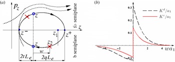
(a) A closed orbit in the
 $zp_{z}$
plane, with observation points
 $z$
(open circles) and collision points (crosses); note
 $w=2L_{e}q_{0}$
and other coordinates
 $q$
and
 $t$
and open orbits are shown by the dashed lines; (b) the kernel parts, direct
 $K^{d}/a_{1}$
and circulating
 $K^{c}/a_{1}$
versus
 $wa_{1}$
, in the case
 $v_{1}/a_{1}=-0.4$
,
 $v_{2}/a_{1}^{2}=-0.2$
and
 $a_{1}{\it\lambda}=2.5$
(which gives
 $c_{d}=1$
).

2.1. Reversal points of each orbit
Let
 $P_{y}^{D}$
be the value of
 $P^{y}$
corresponding to a trajectory with
 $z$
constant (called an equilibrium orbit). From the Hamilton equations, we have
 $$\begin{eqnarray}P_{y}^{D}(z)=a(z)+\{v_{,z}(z)/a_{,z}(z)\},\end{eqnarray}$$
which defines a
 $P_{y}^{D}(z)$
function; moreover the function of
 $z$
equal to
 $v_{D}(z)\equiv P_{y}^{D}-a(z)=p_{y}=v_{,z}(z)/a_{,z}(z)$
is also the drift velocity for this equilibrium orbit.
For a generic orbit
 ${\it\gamma}$
, the
 $p_{z}=0$
points are called reversal points, with a maximum of two points,
 $z^{-}$
and
 $z^{+}$
, with
 $z^{-}\leqslant z^{+}$
, see figure 1; orbits with one only reversal point correspond to extracted electrons (with
 $z^{-}$
finite and
 $z^{+}\rightarrow +\infty$
) or to electrons lost into the plasma (with
 $z^{+}$
finite and
 $z^{-}\rightarrow -\infty$
). Orbits with no reversal points, possible in regions with negligible magnetic field or in small sources, are discussed elsewhere (Cavenago Reference Cavenago2008).
Reversal points divide an orbit into two arcs, the forward arc
 ${\it\gamma}^{\,\mathit{fo}}$
with
 $p_{z}\geqslant 0$
and the backward arc
 ${\it\gamma}^{b}$
with
 $p_{z}\leqslant 0$
. The quantity
 $p=p_{y}-v_{D}(z)=P_{y}-P_{y}^{D}$
oscillates as
 $z$
does along an orbit, but its value
 $p^{-}$
at
 $z^{-}$
, that is
 $p^{-}=P_{y}-P_{y}^{D}(z^{-})$
, is a gauge invariant constant of motion and is a measure of deviation from equilibrium orbit; similarly for
 $p^{+}=P_{y}-P_{y}^{D}(z^{+})$
, which is not independent of
 $p^{-}$
.
Let
 $({\it\eta}_{z},{\it\eta}_{y})$
be the values of
 $(p_{z},p_{y})$
just after a collision at point
 $z_{2}$
, and
 $h_{2}$
be the Hamiltonian at this orbit point. We relate
 ${\it\eta}_{y}$
to
 $p_{y}$
at an observation point
 $z$
by
 $$\begin{eqnarray}p+v_{D}(z)=p_{y}=P_{y}-a(z)=P_{y}-a(z_{2})-\bar{a}={\it\eta}_{y}-\bar{a},\end{eqnarray}$$
with the shorthand for the potential differences
 $\bar{a}=a(z)-a(z_{2})$
and
 $\bar{v}=v(z)-v(z_{2})$
. Since
 $h_{2}=h$
we also have
 ${\it\eta}_{z}=\pm \sqrt{p_{z}^{2}+2V_{e}}$
with the effective potential
 $$\begin{eqnarray}V_{e}(z,z_{2},p)=h_{2}-\frac{{\it\eta}_{y}^{2}+p_{z}^{2}}{2}-v(z_{2})=\bar{v}+\frac{1}{2}\bar{a}^{2}-\bar{a}{\it\eta}_{y}=\bar{v}-\frac{1}{2}\bar{a}^{2}-\bar{a}(p+v_{D}(z)).\end{eqnarray}$$
2.2. Integration of the kinetic equation on orbits
Integrating equation (2.2) along an orbit arc (for example the forward arc), from point
 $z_{1}$
to point
 $z$
for
 $p_{z}\geqslant 0$
, we obtain
 $$\begin{eqnarray}f(z,p_{z},P_{y})=f(z_{1},p_{z}^{{\it\gamma}},P_{y})\text{e}^{-(|z_{1}-z|)/{\it\lambda}}+\int _{z_{1}}^{z}\,\text{d}z_{2}\,\text{e}^{-(|z-z_{2}|)/{\it\lambda}}\frac{2j_{a}(z_{2})}{{\it\lambda}}G^{{\it\gamma}},\end{eqnarray}$$
with
 $z\geqslant z_{2}\geqslant z_{1}\geqslant z^{-}$
and
 $p_{z}^{{\it\gamma}}=p_{z}$
at
 $z_{1}$
determined by the orbit; the scattering factor
 $$\begin{eqnarray}G^{{\it\gamma}}\equiv \frac{f_{g}({\it\eta}_{z})f_{g}({\it\eta}_{y})}{c_{{\rm\pi}}}=\frac{\text{e}^{v(z_{2})-h_{2}}}{2\sqrt{2{\rm\pi}}}=\frac{\text{e}^{-\bar{v}-(1/2)(p_{z}^{2}+p_{y}^{2})}}{2\sqrt{2{\rm\pi}}}{\it\theta}_{C}=G(z,p_{z},P_{y};z_{2}),\end{eqnarray}$$
can be transformed from a function of
 ${\it\eta}_{z},{\it\eta}_{y}$
to a function of
 $\boldsymbol{p}$
,
 $z$
and
 $z_{2}$
as shown, thanks to the
 $h=h_{2}$
energy conservation, represented by the factor
 ${\it\theta}_{C}$
, equal to zero when
 $z,\boldsymbol{p}$
and
 $z_{2}$
,
 $\boldsymbol{{\it\eta}}$
are not on the same orbit and equal to one if they are. A convenient formula is
 ${\it\theta}_{C}={\rm\Theta}(p_{z}^{2}+2V_{e}){\rm\Theta}(z_{2}-z^{-}){\rm\Theta}(z^{+}-z_{2})$
. The expression for
 $f$
on the backward arc is similar to (2.8), with
 $z\leqslant z_{2}\leqslant z_{1}\leqslant z^{+}$
, the integration limits reversed and the same
 $G$
, since
 $G$
is even in
 $p_{z}$
. For
 $z_{1}=z^{+}$
we obtain
 $$\begin{eqnarray}f(z,p_{z}\leqslant 0,P_{y})=f(z^{+},0,P_{y})\text{e}^{(z-z^{+})/{\it\lambda}}+\int _{z}^{z^{+}}\,\text{d}z_{2}\,\text{e}^{(z-z_{2})/{\it\lambda}}\frac{2j_{a}(z_{2})}{{\it\lambda}}G^{{\it\gamma}}.\end{eqnarray}$$
2.3. The recirculation effect
When an orbit has two reversal points, which is the most common case in sources much larger than the Larmor radius, the orbit is closed and electrons may recirculate from
 $z^{-}$
to
 $z^{+}$
and vice versa, if not scattered during travel. Using (2.8) in the case
 $z=z^{+}$
and
 $z_{1}=z^{-}$
we find:
 $$\begin{eqnarray}f(z^{+},0,P_{y})=f(z^{-},0,P_{y})\text{e}^{-s_{d}}+\int _{z^{-}}^{z^{+}}\,\text{d}z_{2}\,\text{e}^{(z_{2}-z^{+})/{\it\lambda}}G(z^{+},0,P_{y};z_{2})\frac{2j_{a}(z_{2})}{{\it\lambda}},\end{eqnarray}$$
with
 $s_{d}=(z^{+}-z^{-})/{\it\lambda}$
. Similarly substituting
 $z=z^{-}$
in (2.10) for the
 $p_{z}\leqslant 0$
arc,
 $$\begin{eqnarray}f(z^{-},0,P_{y})=f(z^{+},0,P_{y})\text{e}^{-s_{d}}+\int _{z^{-}}^{z^{+}}\,\text{d}z_{2}\,\text{e}^{(z^{-}-z_{2})/{\it\lambda}}G(z^{-},0,P_{y};z_{2})\frac{2j_{a}(z_{2})}{{\it\lambda}}.\end{eqnarray}$$
For any fixed
 $z_{2}$
, we can apply (2.9) twice, once with
 $z=z^{-}$
and the other time with
 $z=z^{+}$
, so proving the equalities
 $$\begin{eqnarray}G^{{\it\gamma}}=G(z^{-},0,P_{y};z_{2})=G(z^{+},0,P_{y};z_{2})={\textstyle \frac{1}{2}}{\it\theta}_{C}\text{e}^{v(z_{2})-v(z^{\pm })}f_{g}(p^{\pm }+v_{D}(z^{\pm })),\end{eqnarray}$$
since
 $p_{z}=0$
at reversal points and
 $p_{y}$
may be expressed with (2.6). Solving the (2.11) and (2.12) system for
 $f(z^{\pm },0,P_{y})$
and rearranging we obtain
 $$\begin{eqnarray}f(z^{-},0,P_{y})=\frac{2}{{\it\lambda}}\int _{z^{-}}^{z^{+}}\,\text{d}z_{2}\,R^{-}G^{{\it\gamma}}j_{a}(z_{2}),\quad f(z^{+},0,P_{y})=\frac{2}{{\it\lambda}}\int _{z^{-}}^{z^{+}}\,\text{d}z_{2}\,R^{+}G^{{\it\gamma}}j_{a}(z_{2}),\end{eqnarray}$$
with the response factors
 $$\begin{eqnarray}R^{+}=\frac{\cosh ((z_{2}-z^{-})/{\it\lambda})}{\sinh s_{d}},\quad R^{-}=\frac{\cosh ((z_{2}-z^{+})/{\it\lambda})}{\sinh s_{d}}.\end{eqnarray}$$
We may rewrite these as
 $R^{-}=R(z^{-}-z_{2})$
and
 $R^{+}=R(z^{+}-z_{2})$
with the response function
 $$\begin{eqnarray}R(x)=\exp \left(-\frac{|x|}{{\it\lambda}}\right)+\cosh \left(\frac{x}{{\it\lambda}}\right)\frac{\text{e}^{-s_{d}}}{\sinh s_{d}}.\end{eqnarray}$$
Let
 $R^{d}$
be the first term above and
 $R^{c}$
the second term. Note that
 $R^{d}$
is the expression obtained neglecting recirculation (Cavenago Reference Cavenago2008). For
 ${\it\lambda}\rightarrow 0$
, with
 $z^{+}-z^{-}$
fixed, we have
 $s_{d}\rightarrow \infty$
and
 $R/R^{d}$
converges to
 $1$
. Thus
 $R^{d}$
is the no-recirculation response (or direct response) and
 $R^{c}$
expresses the additional effect of recirculation, which has a pole for
 ${\it\lambda}\rightarrow \infty$
(cancelled by the
 $2/{\it\lambda}$
factor in (2.14)), as expected.
2.4. The kernel
 $K$

The Lorentz force is
 $-h_{,z}=p\,a_{,z}$
thanks to (2.6). With no loss of generality, we assume
 $a_{,z}>0$
; so we have
 $p>0$
at a
 $z^{-}$
point (since it is a minimum of
 $z$
on the orbit), and
 $p<0$
at a
 $z^{+}$
point. We now substitute (2.14) into (2.4), changing the integration variable from
 $P_{y}$
to
 $p$
; since (2.13) and (2.16) hold, exchanging
 $p$
and
 $z_{2}$
integrations we find (1.1) with a kernel
 $$\begin{eqnarray}K(z_{2}-z;z;a,v)=\frac{1}{2}a_{,z}\text{e}^{v(z_{2})-v(z)}\int _{-\infty }^{\infty }\,\text{d}p\,{\it\theta}_{C}^{0}R(z-z_{2})pf_{g}(p+v_{D}(z)),\end{eqnarray}$$
where
 ${\it\theta}_{C}^{0}$
is
 ${\it\theta}_{C}$
at
 $p_{z}=0$
; this factor implicitly selects the
 $p$
integration domain
 $D^{1}$
according to the (2.14) integration limits. It is convenient to introduce the quantity
 $w=z_{2}-z$
to compute the domain
 $D_{w}^{1}(p)$
, as detailed in appendix A, with results:
 $$\begin{eqnarray}D_{w}^{1}(p)=\{s_{w}p\geqslant \max (0,s_{w}q_{0})\},\quad q_{0}(w)=(\bar{v}/\bar{a})-{\textstyle \frac{1}{2}}\bar{a}-v_{d},\end{eqnarray}$$
where we introduced the shorthand
 $s_{w}=\text{sign}(w)$
and
 $v_{d}=v_{D}(z)$
. For example, at any fixed
 $z$
the local second-order approximation is defined by:
 $$\begin{eqnarray}v(z+w)=v_{0}+v_{1}w+{\textstyle \frac{1}{2}}v_{2}w^{2}+O(w)^{3},\quad a(z+w)\cong a_{0}+a_{1}w+O(w)^{3},\end{eqnarray}$$
where the variations of the coefficients
 $a_{1}$
and
 $v_{2}=v^{\prime \prime }(z)$
are assumed zero or adiabatically slow with
 $z$
with respect to the fast oscillations of orbit with
 $w$
; note
 $a_{1}=a^{\prime }(z)>0$
and
 $a_{2}=0$
. We have
 $v_{d}=v_{1}/a_{1}$
and
 $q_{0}(w)=w/(2L_{e})$
with
 $L_{e}=a_{1}/(a_{1}^{2}+v_{2})$
an effective Larmor radius. Also it results in
 $z^{+}-z^{-}=2L_{e}|p^{-}|$
and
 $p^{+}=-p^{-}$
, which clearly shows that the oscillation width is
 $2L_{e}$
for
 $p=1$
. In this example, when
 $v_{2}+a_{1}^{2}>0$
all orbits are closed and the integration domain
 $D^{1}$
is simply
 $p/w\geqslant 1/(2L_{e})$
. When
 $v_{2}+a_{1}^{2}<0$
, the effective Larmor radius is negative, indicating instability of the equilibrium orbit, and the domain
 $D^{1}$
is simply
 $p/w\geqslant 0$
.
2.5. The kernel
$N$

We calculate first
 $n_{a}^{b}$
, that is the density due to backward moving particles:
 $n_{a}^{b}=\int ^{\prime }f{\rm\Theta}(-p_{z})=(2/{\it\lambda})\int \,\text{d}z_{2}\,N^{b}j_{a}$
with the kernel part
 $N^{b}$
. Then we will use symmetry to calculate the density contribution of the forward flow:
 $n_{a}^{\,\mathit{fo}}=\int ^{\prime }f{\rm\Theta}(p_{z})=(2/{\it\lambda})\int \,\text{d}z_{2}\,N^{\,\mathit{fo}}j_{a}$
, where
 $N^{\,\mathit{fo}}$
is the other part of the kernel
 $N$
. We consider all orbits closed. Using
 $f$
value from (2.10) and exchanging the order of integration, we find
 $$\begin{eqnarray}N^{b}(w;z;a,v)=\int \,\text{d}p_{y}\int _{-\infty }^{0}\,\text{d}p_{z}[\text{e}^{-w/{\it\lambda}}{\rm\Theta}(w)+\text{e}^{-w^{+}/{\it\lambda}}R(w^{+}-w)]G(z,p_{z},P_{y};z+w),\end{eqnarray}$$
with the shorthand
 $w^{+}=z^{+}-z$
and
 $w^{-}=z^{-}-z$
and integration domain restricted by the
 ${\it\theta}_{C}$
factor in
 $G$
. Transformation from
 $p_{y},p_{z}$
to quantities
 $$\begin{eqnarray}q={\textstyle \frac{1}{2}}(p-p^{+}),\quad t={\textstyle \frac{1}{2}}(p^{-}-p),\end{eqnarray}$$
(where
 $t$
from this point is not the time) is useful for calculating
 $N^{b}$
, at least with (2.19) potential; transformation and domains
 $D_{w}^{2}(q,t)$
and
 $D_{w}^{3}(p_{z},p_{y})$
are calculated in (A 3), (A 4) and (A 6). Expanding
 $G$
, note that
 $N^{b}$
can be factorized as
 $N^{b}=k_{a}\text{e}^{-\bar{v}}{\check{N}}^{b}$
with
 $$\begin{eqnarray}{\check{N}}^{b}(w;c_{1},v_{d},c_{d})=\int _{D_{w}^{2}}\,\text{d}q\,\text{d}t\frac{q+t}{\sqrt{qt}}[\text{e}^{-c_{d}q_{0}}{\rm\Theta}(w)+\text{e}^{-c_{d}q}R(c_{d}(q-q_{0}))]E_{1},\end{eqnarray}$$
where
 $E_{1}=\text{e}^{-{\textstyle \frac{1}{2}}(q^{2}+t^{2}+v_{d}^{2})-c_{1}qt-v_{d}(q-t)}$
and
 $k_{a}=((L_{e}a_{1}/2{\rm\pi})^{1/2})/2$
; the dependence on
 $a$
and
 $v$
is now expressed by the parameters
 $c_{1}=2L_{e}a_{1}-1$
,
 $v_{d}$
and
 $c_{d}=2L_{e}/{\it\lambda}$
. The integral for
 $N^{\,\mathit{fo}}$
is as (2.22), but with
 $t$
instead of
 $q$
in the square bracket factor. The symmetry
 $S_{1}$
sends
 $w$
into
 $-w$
and
 $v_{d}$
into
 $-v_{d}$
as explained at the end of appendix A and the domain change due to symmetry is equivalent to the exchange of
 $q$
and
 $t$
in the integral above; so we have
 $$\begin{eqnarray}\displaystyle N^{\,\mathit{fo}}=k_{a}\text{e}^{-\bar{v}}{\check{N}}^{\,\mathit{fo}},\quad {\check{N}}^{\,\mathit{fo}}(w;c_{1},v_{d},c_{d})={\check{N}}^{b}(-w;c_{1},-v_{d},c_{d}). & & \displaystyle\end{eqnarray}$$
3. Kernels and damped partial waves
In this section, we simplify the kernel
 $N$
calculation and give approximated analytic results for the kernel
 $K$
, developing a common approach for both.
For simplicity, we consider (2.19) potentials. Note that the non-recirculating part
 $K^{d}$
can be exactly calculated and is proportional to the
 $\text{e}^{-|z-z_{2}|/{\it\lambda}}M_{,z}$
calculated for more general examples elsewhere (Cavenago Reference Cavenago2008), while the non-recirculating part of
 $N$
corresponds to
 $\text{e}^{-|z-z_{2}|/{\it\lambda}}N$
there. To approximate
 $K^{c}$
we note first the tight upper bound
 $b_{2}(x)$
of
 $$\begin{eqnarray}b(x)=x\text{e}^{-x}/\!\sinh x\leqslant 2x\text{e}^{-2x}+\text{e}^{-3x}\equiv b_{2}(x)\end{eqnarray}$$
for
 $0\leqslant x\leqslant \infty$
. The so-called damped partial waves
 $\text{e}^{-2x}$
and
 $\text{e}^{-3x}$
will make analytic calculations possible, and notwithstanding that we use only two terms, we obtain a good approximation for the whole range discussed. Replacing
 $b(c_{d}p)$
with
 $b_{2}(c_{d}p)$
in (2.17),
 $K$
becomes the sum of five terms of the form
 $\hat{K}_{n;k}^{i}$
defined as
 $$\begin{eqnarray}\hat{K}_{n;k}^{i}(q_{0},v_{d},c_{d})=\frac{1}{2}\text{sign}(q_{0})\text{e}^{-ic_{d}|q_{0}|}\int _{|q_{0}|}^{\infty }\,\text{d}p\,p^{n}\text{e}^{-kc_{d}p}f_{g}(ps_{0}+v_{d}),\end{eqnarray}$$
with
 $s_{0}=\text{sign}(q_{0})$
, typical values of indexes
 $n=0,1$
,
 $i=\pm 1$
and
 $k=0,2,3$
; where the index separator ‘;’ is usually dropped. In detail,
 $K=K^{d}+K^{c}$
and
 $$\begin{eqnarray}\displaystyle & \displaystyle K^{d}(w;z;v_{d},c_{d})=a_{,z}\text{e}^{-\bar{v}}\hat{K}_{10}^{1}(w/2L_{e},v_{d},c_{d}), & \displaystyle\end{eqnarray}$$
 $$\begin{eqnarray}\displaystyle & \displaystyle K^{c}\cong a_{,z}\text{e}^{-\bar{v}}\left[\hat{K}_{12}^{1}\left(\frac{w}{2L_{e}},v_{d},c_{d}\right)+\hat{K}_{12}^{-1}+\frac{\hat{K}_{03}^{1}+\hat{K}_{03}^{-1}}{2c_{d}}\right], & \displaystyle\end{eqnarray}$$
 $t_{0}\geqslant 0$
and for any
 $s$
as
 $$\begin{eqnarray}f_{n}(t_{0},s)=\int _{t_{0}}^{\infty }\,\text{d}t\,t^{n-(1/2)}\text{e}^{-ts-(1/2)t^{2}},\quad\end{eqnarray}$$
whose exact values are listed in appendix B when known, is convenient to express
 $\hat{K}$
, and it also helps for
 ${\check{N}}$
. For
 $q_{0}\geqslant 0$
we can write
 $$\begin{eqnarray}\hat{K}_{nk}^{i}(q_{0},v_{d},c_{d})={\textstyle \frac{1}{2}}\text{e}^{-ic_{d}q_{0}}f_{g}(v_{d})f_{n+(1/2)}(q_{0},v_{d}+kc_{d}),\end{eqnarray}$$
with
 $f_{n+(1/2)}$
given by (B 3) in terms of the complementary error function
 $\text{erfc}(x)=1-\text{erf}(x)$
; for
 $q_{0}<0$
the symmetry property
 $\hat{K}_{nk}^{i}(q_{0},v_{d},c_{d})=-\hat{K}_{nk}^{i}(-q_{0},-v_{d},c_{d})$
is used. Note that
 $\hat{K}$
is discontinuous at
 $q_{0}=0$
, see figure 1(b); the pole of
 $c_{d}$
was previously discussed. From (B 5) we see that
 $\hat{K}_{nk}^{i}$
is asymptotically bounded by
 $\exp [-(i+k)|q_{0}|c_{d}]$
for large
 $w$
(with a strong safety factor
 $\text{e}^{-q_{0}^{2}/2}$
), so the
 $i=-1$
effect is dominated by
 $k=2$
and
 $K_{12}^{-1}$
is as damped as
 $K_{10}^{1}$
.
3.1. Calculation of density kernel N
To exploit the partial waves formula (3.1), we define the density terms
 $$\begin{eqnarray}\hat{N}_{nk;m}^{i}(q_{0};c_{1},v_{d},c_{d})=\text{e}^{ic_{d}q_{0}}\int _{D_{w}^{2}}\,\text{d}q\,\text{d}t\frac{(q+t)^{n}}{\sqrt{qt}}E_{1}\text{e}^{-kc_{d}(q+t)-mc_{d}(q-t)},\end{eqnarray}$$
with
 $E_{1}$
given after (2.22); from it, the kernel part
 ${\check{N}}^{b}$
, thanks to (3.1) and (A 5), becomes
 $$\begin{eqnarray}{\check{N}}^{b}(w,c_{1},v_{d},c_{d})\cong {\rm\Theta}(w)\hat{N}_{10;0}^{-1}+\hat{N}_{12;0}^{-1}+\hat{N}_{11;1}^{1}+\hat{N}_{13;1}^{1}+\frac{\hat{N}_{03;0}^{-1}+\hat{N}_{04;1}^{1}}{2c_{d}},\end{eqnarray}$$
where all density terms are evaluated at
 $q_{0}=w/2L_{e}$
,
 $c_{1},v_{d},c_{d}$
. The symmetry relation for
 $\hat{N}$
is
 $$\begin{eqnarray}\hat{N}_{nk;m}^{i}(-q_{0},c_{1},v_{d},c_{d})=\hat{N}_{nk;-m}^{-i}(q_{0},c_{1},-v_{d},c_{d}).\end{eqnarray}$$
Therefore, in the total density kernel (backward plus forward parts)
 $$\begin{eqnarray}\displaystyle N(w;z;c_{1},v_{d},c_{d}) & = & \displaystyle k_{a}\text{e}^{-\bar{v}} [\hat{N}_{10;0}^{-s_{w}}+\hat{N}_{12;0}^{-1}+N_{12;0}^{1}+\hat{N}_{11;-1}^{-1}+\hat{N}_{11;1}^{1}\nonumber\\ \displaystyle & & \displaystyle +\,\hat{N}_{13;-1}^{-1}+\hat{N}_{13;1}^{1}+(2c_{d})^{-1}(\hat{N}_{03;0}^{-1}+\hat{N}_{03;0}^{1}+\hat{N}_{04;-1}^{-1}+\hat{N}_{04;1}^{1})]\qquad \quad\end{eqnarray}$$
all density terms
 $\hat{N}$
are evaluated at
 $q_{0}=w/2L_{e}$
,
 $c_{1},v_{d},c_{d}$
(one change of sign of
 $v_{d}$
from
 ${\check{N}}^{b}$
to
 ${\check{N}}^{\,\mathit{fo}}$
thanks to (2.23) and another change applying (3.9)); the first term, with
 $s_{w}=\text{sign}(w)$
, includes the first terms of
 ${\check{N}}^{b}$
and of
 ${\check{N}}^{\,\mathit{fo}}$
.
In (3.7), for
 $q_{0}\geqslant 0$
the integration on
 $t$
runs from 0 to
 $\infty$
so it can be performed analytically with (3.5), obtaining an intermediate computation step:
 $$\begin{eqnarray}\hat{N}_{nk;m}^{i}(q_{0};c_{1},v_{d},c_{d})=\text{e}^{ic_{d}q_{0}-(v_{d}^{2}/2)}\int _{q_{0}}^{\infty }\,\text{d}q\,\text{e}^{-qs^{+}-(q^{2}/2)}g_{n}(c_{1}q+s^{-},q),\end{eqnarray}$$
with the shorthand
 $s^{-}=(k-m)c_{d}-v_{d}$
and
 $s^{+}=(k+m)c_{d}+v_{d}$
; the functions
 $g_{0}(x,q)=f_{0}(0,x)$
and
 $g_{1}(x,q)=f_{1}(0,x)+qf_{0}(0,x)$
are given by (B 4); in general the integration of
 $q$
should be obtained numerically. For
 $q_{0}<0$
, the symmetry relation is used. For
 $q_{0}=0$
and
 $c_{1}=1$
a good approximation is reported in (B 6).
3.2. Moments of the kernels
$K$
and
$N$


Since
 $K$
has positive and negative values, initial information on its effect is given by
 $\int \!\,\text{d}w\,K$
, or in general by the
 $\ell$
th moment
 ${\mathcal{K}}_{\ell }=\int \,\text{d}w\,Kw^{\ell }/\ell !$
with integer
 $\ell \geqslant 0$
. We first calculate the integral moments term by term in the
 $w>0$
range
 $$\begin{eqnarray}\text{}^{+}\hat{{\mathcal{K}}}_{nk}^{\ell i}(v_{d},c_{d})=a_{1}\int _{0}^{\infty }\,\text{d}w\,\text{e}^{-\bar{v}}\frac{w^{\ell }}{\ell !}\hat{K}_{nk}^{i}\left(\frac{w}{2L_{e}},v_{d},c_{d}\right);\end{eqnarray}$$
the similar integral
 $^{-}\hat{{\mathcal{K}}}_{nk}^{\ell i}$
on the
 $w<0$
range satisfies the symmetry property
 $$\begin{eqnarray}\text{}^{-}\hat{{\mathcal{K}}}_{nk}^{\ell i}(v_{d},c_{d})=(-1)^{\ell +1}\times ^{+}\hat{{\mathcal{K}}}_{nk}^{\ell i}(-v_{d},c_{d});\end{eqnarray}$$
their sum is
 $\hat{{\mathcal{K}}}_{nk}^{\ell i}\equiv \text{}^{-}\hat{{\mathcal{K}}}_{nk}^{\ell i}+{\text{}^{+}\hat{{\mathcal{K}}}}_{nk}^{\ell i}$
. Exact calculation is possible in the
 $v_{2}=0$
case (that is
 $c_{1}=1$
): first by changing the integration variable to
 $y=w/2L_{e}$
we obtain
 $$\begin{eqnarray}\text{}^{+}\hat{{\mathcal{K}}}_{nk}^{\ell i}=a_{1}(2L_{e})^{\ell +1}\int _{0}^{\infty }\,\text{d}y\,\text{e}^{-c_{y}y}y^{\ell }\int _{y}^{\infty }\,\text{d}p\,\frac{1}{2}p^{n}\text{e}^{-kc_{d}p}f_{g}(p+v_{d})/\ell !,\end{eqnarray}$$
with
 $c_{y}=ic_{d}-2L_{e}a_{1}v_{d}$
. Exchanging the
 $y$
and
 $p$
integration order, the integration on
 $y$
is elementary and gives
 $$\begin{eqnarray}\int _{0}^{p}\,\text{d}y\frac{y^{\ell }}{\ell !}\exp (-c_{y}y)=c_{y}^{-\ell -1}\left[1-\text{e}^{-c_{y}p}\mathop{\sum }_{{\it\nu}=0}^{{\it\nu}=\ell }\frac{(c_{y}p)^{{\it\nu}}}{{\it\nu}!}\right].\end{eqnarray}$$
Now we define the value
 $\tilde{k}(c_{y})=k+(c_{y}/c_{d})$
, which is real since
 $c_{d}>0$
, while the index
 $k$
was an integer; note that the
 $\hat{K}_{n;\tilde{k}}^{0}(0,v_{d},c_{d})$
integrand contains a factor
 $\text{e}^{-c_{y}p-kc_{d}p}$
and the same factor appears by substituting (3.15) into (3.14). This allows us to write
 $\text{}^{+}\hat{{\mathcal{K}}}_{nk}^{\ell i}$
with known functions
 $$\begin{eqnarray}\text{}^{+}\hat{{\mathcal{K}}}_{nk}^{\ell i}=a_{1}\left(\frac{2L_{e}}{c_{y}}\right)^{\ell +1}\left[\hat{K}_{nk}^{0}(0,v_{d},c_{d})-\mathop{\sum }_{{\it\nu}=0}^{{\it\nu}=\ell }\frac{(-c_{y})^{{\it\nu}}}{{\it\nu}!}{{\mathcal{O}}_{c}}^{{\it\nu}}\hat{K}_{n;\tilde{k}(c_{y})}^{0}(0,v_{d},c_{d})\right],\end{eqnarray}$$
with the differential operator
 ${\mathcal{O}}_{c}\equiv \partial /\partial c_{y}$
. For example
 $$\begin{eqnarray}\text{}^{+}\hat{{\mathcal{K}}}_{nk}^{1i}(v_{d},c_{d})=a_{1}(2L_{e}/c_{y})^{2}[\hat{K}_{nk}^{0}(0,v_{d},c_{d})-\hat{K}_{n;\tilde{k}}^{0}(0,v_{d},c_{d})-c_{y}\hat{K}_{n+1;\tilde{k}}^{0}].\end{eqnarray}$$
Moments
 ${\mathcal{K}}_{\ell }=\int \,\text{d}w\,Kw^{\ell }/\ell !$
simply correspond to the sum of the terms from (3.4) and (3.3), using (3.16) and (3.6) and satisfy the symmetry
 ${\mathcal{K}}_{\ell }(-v_{d},c_{d})=(-1)^{\ell +1}{\mathcal{K}}_{\ell }(v_{d},c_{d})$
.
The case
 $v_{2}\not =0$
can be studied with a power series in
 $v_{2}$
. We prefix a label
 $\text{}^{0}$
to
 ${\mathcal{K}}$
to indicate moments calculated at
 $v_{2}=0$
and a label
 $\text{}^{2}$
to indicate the expansion in powers of
 $v_{2}$
as
 $\text{}^{2}{\mathcal{K}}_{\ell }=\text{}^{0}{\mathcal{K}}_{\ell }+(v_{2}(\ell +2)(\ell +1)\;\text{}^{0}{\mathcal{K}}_{\ell +2})/2+O(v_{2})^{2}$
.
The same considerations apply for the moments of
 $N$
, defined as
 ${\mathcal{N}}_{\ell }(c_{1},v_{d},c_{d})=\int \,\text{d}w\,Nw^{\ell }/\ell !$
, whose term by term calculation reduces to (B 6).
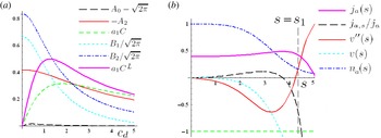
(a) Density factors
 $A_{0}-\sqrt{2{\rm\pi}}$
and
 $-A_{2}$
and
 $B_{1}/\sqrt{2{\rm\pi}}$
and
 $B_{2}/\sqrt{2{\rm\pi}}$
and the conductivity factors
 $a_{1}C$
and
 $a_{1}C^{L}$
, as functions of the parameter
 $c_{d}$
; (b) tracing of
 $j_{a}(s)$
solution from (4.7), with
 $j=0.05$
and
 $c_{d}(0)=1.0$
; potential
 $v(s)$
and density
 $n_{a}(s)$
and criteria
 $v^{\prime \prime }(s)\geqslant -1$
and
 $|j_{a,s}/j_{a}|\ll 1$
are also shown.

4. Approximations of integral equation solution
First we study the quasi-equilibrium solution, where
 $j_{a}$
is constant, that is
 $j_{a,z}=0$
; this allows for an electric field, but a constant electric field, that is
 $v_{2}=0$
everywhere. Then
 $c_{1}=1$
and
 $2/{\it\lambda}=a_{1}c_{d}$
. From (1.1) and § 3 and especially (3.16), we find
 $$\begin{eqnarray}\frac{j}{j_{a}}=4\int \,\text{d}w\,K=4^{0}{\mathcal{K}}_{0}=-v_{d}c_{d}\left[1-\left(\frac{4}{3}+\frac{1}{4}v_{d}^{2}\right)c_{d}^{2}+O(c_{d})^{3}\right],\end{eqnarray}$$
where the series expansion in
 $c_{d}$
is the strong recirculation limit and simplifies the long analytic expression of
 $\text{}^{0}{\mathcal{K}}_{0}$
, given in (B 9). Similarly, from (1.2)
 $$\begin{eqnarray}\frac{n_{a}}{j_{a}}=\frac{2}{{\it\lambda}}\int \,\text{d}w\,N=\frac{{\rm\pi}}{v_{d}}\text{erf}\frac{v_{d}}{\sqrt{2}}+A_{22}(v_{d})c_{d}^{2}+\frac{7{\rm\pi}(3+v_{d}^{2})}{12}c_{d}^{3}+O(c_{d})^{4},\end{eqnarray}$$
with coefficient
 $A_{22}(v_{d})\cong \sqrt{2{\rm\pi}}[(1/3)+(11v_{d}^{2}/160)+O(v_{d}^{4})]$
. Note that
 $n_{a}/j_{a}\cong \sqrt{2{\rm\pi}}$
within second-order terms, so that (4.1) shows that current is proportional to
 $-v_{1}n_{a}$
; we define a conductivity (in scaled units) as
 $$\begin{eqnarray}C=-\!\left(\frac{\partial j/n_{a}}{\partial v_{1}}\right)_{v_{1}=0}=\frac{c_{d}-c_{5}c_{d}^{3}}{a_{1}\sqrt{2{\rm\pi}}}+O(c_{d}^{4})=\frac{(8/{\rm\pi})^{1/2}}{a_{1}c_{d}}-\frac{8}{{\rm\pi}a_{1}c_{d}^{2}}+O(c_{d}^{-3}),\end{eqnarray}$$
where
 $c_{5}=5/3$
and we show two expansions of
 $C$
, one for small
 $c_{d}$
values, the other for
 $c_{d}\rightarrow \infty$
(last step). For all
 $c_{d}$
values, the quantity
 $a_{1}C$
(which is dimensionless) is shown in figure 2, together with the density factors
 $A_{0}$
and
 $A_{2}$
, which are defined by the
 $n_{a}/j_{a}=A_{0}(c_{d})+A_{2}(c_{d})v_{d}^{2}+O(v_{d}^{4})$
expansion.
The typical result from fluid equations (Lieberman & Lichtenberg Reference Lieberman and Lichtenberg1994) for the electron mobility
 ${\it\mu}_{e}$
as a function of the collision frequency
 ${\it\nu}_{m}$
(also sometimes referred as a Chapman–Cowling like formula (Tsuda, Fukao & Maeda Reference Tsuda, Fukao and Maeda1969)) must be represented, in the units used here for conductivity
 $C$
, as
 $C^{L}={\it\mu}_{e}mv_{th}/e$
where
 $v_{th}=\sqrt{T_{0}/m}$
, as previously defined. With
 ${\it\nu}_{m}=k_{1}v_{th}/{\it\lambda}$
and
 $k_{1}$
a numerical factor of approximately one, we find
 $a_{1}C^{L}=2k_{1}c_{d}/(4+c_{d}^{2}k_{1}^{2})$
.
This quantity
 $a_{1}C^{L}$
is plotted in figure 2 with
 $k_{1}=(8/{\rm\pi})^{1/2}$
(the value for a hard sphere model). Even if
 $C$
and
 $C^{L}$
display similar behaviour for
 $c_{d}\rightarrow 0$
and
 $c_{d}\rightarrow \infty$
, note that
 $C$
results up to 40 % less than
 $C^{L}$
for intermediate regimes. Corrections to
 ${\it\mu}_{e}$
(and
 $C^{L}$
) formula for crossed electric and magnetic fields were proposed elsewhere (Tsuda et al.
Reference Tsuda, Fukao and Maeda1969; Daniłko & Barral Reference Daniłko and Barral2015), with numerical simulations and physical reasoning based on kinetic effects; there, mobility
 ${\it\mu}_{e}$
increases or decreases depending on
 $v_{d}$
and electron temperature. In view of the motivations here, following (2.3), we may consider
 $k_{1}$
as an adjustable parameter, which determines
 ${\it\lambda}$
in terms of the collision frequency
 ${\it\nu}_{m}$
. For the
 $c_{d}\rightarrow 0$
limit, we obtain
 $C^{L}\cong (k_{1}c_{d}/a_{1})/2$
so that
 $C$
matches
 $C^{L}$
with
 $k_{1}=(2/{\rm\pi})^{1/2}$
. For
 $c_{d}\rightarrow \infty$
, we find
 $C^{L}\cong 2/(k_{1}c_{d}a_{1})$
so that
 $C$
matches
 $C^{L}$
with
 $k_{1}=({\rm\pi}/2)^{1/2}$
, which value is not very different from
 $(8/{\rm\pi})^{1/2}$
. Whilst further investigations are certainly worthwhile, some partial agreement between
 $C$
and
 $C^{L}$
is already evident.
4.1. Integral equation for
$j_{a}$
and presheath

Equation (1.1) can be formally expanded as
 $$\begin{eqnarray}y(z)\equiv \frac{{\it\lambda}}{2}j_{a,z}+\frac{1}{4}j=\int \,\text{d}w\,K(w;z)j_{a}(w+z)\cong \mathop{\sum }_{n=0}^{\infty }{\mathcal{K}}_{n}j_{a}^{(n)}(z),\end{eqnarray}$$
when the variation of
 $K$
with
 $z$
(due to variation of
 $v_{0}$
,
 $v_{1}$
and
 $v_{2}$
with
 $z$
) is much slower than the variation due to
 $w$
, with the typical scale length
 $L_{e}$
, so that the fast
 $w$
spatial scale can be integrated out. Moments satisfy
 ${\mathcal{K}}_{n}\propto L_{e}^{n}\propto (a_{1})^{-n}$
from dimensional analysis, so that higher-order derivatives
 $j_{a}^{(n)}(z)$
should be bounded by
 $({\it\beta}_{0}a_{1})^{n}$
with a constant
 ${\it\beta}_{0}<1$
for the convergence of sum. This defines the presheath conditions, matching
 $j_{a}$
constant at a given
 $z=z_{p}$
(which may goes to
 $-\infty$
). By restricting the sum index as
 $n\leqslant n_{T}$
, with
 $n_{T}$
a given integer, we obtain an ODE that can be numerically traced up to some
 $z_{0}$
; the region
 $z\leqslant z_{1}$
of validity of the solution (depending on
 $n_{T}$
and
 $v(z)$
) has to checked case by case, and is smaller than the traced solution:
 $z_{1}<z_{0}$
. We use a combination of criteria
 $a_{1}^{2}+v_{2}>0$
(which translates to
 $E_{z,z}>-eB_{x}^{2}/m$
) and
 $|j_{a,z}/j_{a}a_{1}|<1$
to estimate
 $z_{1}$
; results for the
 $n_{T}=3$
case are shown in examples later.
To improve
 ${\mathcal{K}}_{n}$
convergence, we introduce the so-called regularization technique. Let us define the operators
 $$\begin{eqnarray}{\mathcal{O}}_{2}^{z}=a-b\partial _{z}+c{\partial _{z}}^{2},\quad {\mathcal{O}}_{2}^{w}=a+b\partial _{w}+c{\partial _{w}}^{2}\end{eqnarray}$$
and apply
 ${\mathcal{O}}_{2}^{z}$
to the integral form of (4.4), obtaining
 $$\begin{eqnarray}{\mathcal{O}}_{2}^{z}y(z)=[K_{,w}j_{a}+(bj_{a}-j_{a,z})K]_{w=-{\it\epsilon}}^{w={\it\epsilon}}+\unicode[STIX]{x2A0D}_{-\infty }^{\infty }\quad \,\text{d}w\,j_{a}{\mathcal{O}}_{2}^{w}K(w;z),\end{eqnarray}$$
where we consider only the case of
 $a$
and
 $b$
constant and
 $c=1$
for simplicity, and in the last term (named
 $I_{P}$
in the following) the range
 $R_{P}\equiv \{-{\it\epsilon}<w<{\it\epsilon}\}$
, with
 ${\it\epsilon}\rightarrow 0^{+}$
, is excluded from the integration, similarly to a principal value integral.
Applying the operator
 ${\mathcal{O}}_{2}^{z}$
to the sum in (4.4), we find
 $$\begin{eqnarray}{\mathcal{O}}_{2}^{z}y(z)=\frac{1}{4}aj+\frac{{\it\lambda}}{2}(aj_{a}^{\prime }-bj_{a}^{\prime \prime }+j_{a}^{\prime \prime \prime })=\mathop{\sum }_{n=0}^{\infty }\check{{\mathcal{K}}}_{n}j_{a}^{(n)}(z),\end{eqnarray}$$
where the regularized moments are
 $\check{{\mathcal{K}}}_{n}=a{\mathcal{K}}_{n}-b{\mathcal{K}}_{n-1}+{\mathcal{K}}_{n-2}$
with
 ${\mathcal{K}}_{-1}=0={\mathcal{K}}_{-2}$
for convenience.
If
 ${\mathcal{O}}_{2}^{w}K(w;z)=0$
, except for the range
 $R_{P}$
, (4.6) and (4.7) reduce to differential equations, showing also that
 $\check{{\mathcal{K}}}_{n}=0$
for
 $n\geqslant 2$
; such simplification can be achieved (Cavenago Reference Cavenago2008) for the kernel of the purely electrostatic case, with a first order operator
 $c=0$
,
 $b=-v^{\prime }(z)$
and
 $a=(v^{\prime })^{2}+{\it\lambda}^{-1}|v^{\prime }|-v^{\prime \prime }$
. In general,
 ${\mathcal{O}}_{2}^{w}K(w;z)\not =0$
, (4.6) and (4.7) remain integral equations, for which we note some approximate solution methods.
We can simply choose
 $a$
and
 $b$
to make
 ${\mathcal{O}}_{2}^{w}K(w;z)$
much smaller than
 $K$
, especially in regions
 $|w|\geqslant L_{e}$
, in order to decrease regularized moments
 $\check{{\mathcal{K}}}_{n}$
for
 $n>n_{T}=3$
; in detail
 $a$
and
 $b$
are optimized at the initialization of a numerical solver, considering the attenuation lengths of
 $K$
; then (4.7) is solved, keeping only terms up to
 $n\leqslant 3$
in the sum; we call this procedure the regularized solver or the (4.7) solution.


4.2. Coupling to Poisson equation and numerical solutions
The density expression (1.2) is now expanded, keeping up quadratic terms in
 $v_{d}=v_{,z}/a_{1}$
and
 $\partial _{z}$
, and consistently, linear terms in
 $v_{2}=v_{,zz}$
; this requires us to include the
 $\text{}^{2}{\mathcal{N}}_{0}j_{a}=(\text{}^{0}{\mathcal{N}}_{0}+\text{}^{0}{\mathcal{N}}_{2}v_{2})j_{a}$
terms. Changing coordinate to
 $s=a_{1}(z-z_{p})$
, we write the density
 $$\begin{eqnarray}n_{a}=2{\it\lambda}^{-1}[(A_{0}+(v_{,s})^{2}A_{2}+B_{2}v_{,ss})j_{a}+B_{1}v_{,s}j_{a,s}+B_{2}j_{a,ss}],\end{eqnarray}$$
keeping only the
 $v_{,s}$
and
 $v_{,ss}$
dependences explicitly shown; the terms
 $B_{1}(c_{d})$
and
 $B_{2}(c_{d})$
which are defined by the expansions
 $\text{}^{0}{\mathcal{N}}_{1}a_{1}=v_{d}B_{1}+O(v_{d}^{3})$
and
 $\text{}^{0}{\mathcal{N}}_{2}a_{1}^{2}=B_{2}(c_{d})+O(v_{d}^{2})$
are shown in figure 2(a). With the scaled potential
 $v(z)=-e{\it\phi}(z)/T_{0}$
the Poisson equation becomes
 $$\begin{eqnarray}(a_{1}{\it\lambda}_{D})^{2}v_{,ss}=n_{p0}\text{e}^{v(z)}-n_{\text{H}-}-n_{e0}n_{a},\end{eqnarray}$$
where
 ${\it\lambda}_{D}$
is the Debye length and
 $n_{p0}$
and
 $n_{e0}$
are constants, depending on plasma equilibrium at
 $z=z_{p}$
(deep inside the plasma), which we take as a ground reference
 $v=0$
. In this analysis, we set
 $n_{\text{H}-}=0$
, so
 $n_{e0}=1=n_{a}(0)$
and
 $n_{p0}=1$
at
 $s=0$
; moreover the net flow
 $j$
(which is a constant parameter under the
 ${\mathcal{S}}=0$
assumption) is set at a small value. For a perfect equilibrium, from (4.3) we see that
 $v^{\prime }(0)$
is proportional to
 $j$
, thus
 $v^{\prime }(0)=0$
is a suitable boundary condition (bc), producing only a short transient near
 $s=0$
. Other bc are
 $j_{a}^{\prime }=j_{a}^{\prime \prime }=0$
and
 $j_{a}(0)$
as determined by (4.8).
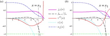
Solutions of the (4.7)–(4.9) system are traced in figures 2 and 3, with a fixed value of the
 $c_{d}(0)=2/(a_{1}{\it\lambda})$
parameter; in these examples we set
 $N_{0}=3.2\times 10^{17}~\text{m}^{-3}$
,
 $T_{0}=1$
eV,
 $j=0.05$
(equivalent to
 $j_{e}=1.1$
kA m
 $^{-2}$
) which are realistic values for intense ion sources. Magnetic flux density
 $B_{x}$
is set to
 $5\times 10^{-4}$
T (a low constant value for simplicity), so that
 $a_{1}=200$
m
 $^{-1}$
. Two values for
 ${\it\lambda}$
were considered:
 ${\it\lambda}=20$
mm (that is
 $c_{d}=0.5$
) and
 ${\it\lambda}=10$
mm that is
 $c_{d}=1.0$
; since
 ${\it\lambda}_{D}=0.014$
mm and thus
 $(a_{1}{\it\lambda}_{D})^{-2}=1.3\times 10^{5}$
is large, charge quasi-neutrality is satisfied up to approximately
 $z_{0}$
(if charge quasi-equilibrium cannot be maintained, the numerical solution breaks up). The criteria for the (4.4) approximation limits the validity of the solutions, at a
 $s_{1}=a_{1}(z_{1}-z_{p})$
shown in figure 3(a); similarly for (4.7), see a comparison in figure 3.
Another method of solution, which avoids truncation of sums of
 $j_{a}^{(n)}$
, is the iterative solution of (4.6): after evaluating the integral term
 $I_{P}$
for a trial solution
 $T_{0}=\{j_{a}(s),v(s),n_{a}(s)\}$
, solving the ODE part of (4.6) gives a new solution
 $T_{1}$
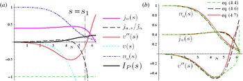
; this procedure is repeated until convergence (typically slow at 30 iterations, since we require 6 digit stability of the
 $z_{0}$
value). The converged solution is shown in figure 4, including the value of the integral term
 $I_{P}(s)$
; note that the final value of
 $I_{P}(s)$
is small, which helps the convergence of the procedure.
For
 $s\leqslant s_{1}$
, we note that
 $j_{a}$
stays roughly constant, while
 $n_{a}$
has to decrease to maintain quasi-neutrality since the proton density decreases with the decrease of potential
 $v(s)$
, and
 $-v^{\prime }(s)$
has to increase for consistency with the conservation of
 $j$
. The
 $v_{,ss}$
term in (4.8) interacts with the Poisson equation (4.9), with stabilizing effects.
The case of
 $B_{x}$
slowly rising towards extraction may be similarly studied.
(a) Solution components as in figure 3(b), but with
 $c_{d}(0)=0.5$
and use of iterative solver from (4.6), showing its integral term
 $I_{P}(s)$
; (b) comparison of solution components
 $n_{a}$
and
 $v_{,ss}$
from three solvers, respectively with (4.6), (4.7) and (4.4); axis
 $s$
origin was shifted to align
 $j_{a}$
.

5. Conclusions, discussion and perspectives
Investigation of a collisional and kinetic model of electron transport in crossed magnetic and electric fields has shown the convenience of expressing the phase density
 $f$
(a function of two velocities and one space coordinate
 $z$
) from an absolute flow density
 $j_{a}$
, a function of the space coordinate
 $z$
only as is the number density
 $n_{a}$
. With the Poisson equation, the IDE for
 $j_{a}$
and
 $n_{a}$
make a closed system. Their kernels
 $K$
and
 $N$
strongly depend on trapped orbits when the effective Larmor radius
 $L_{e}$
is smaller than the mfp
 ${\it\lambda}$
; suitably approximated analytic formulas were here developed for all
 $c_{d}=2L_{e}/{\it\lambda}$
values, in terms of the error function, including moments of
 $K$
and
 $N$
.
When fields are uniform (translation invariance), the IDE can be simply solved, finding a conductivity value that can be compared to the electron mobility from fluid equations.
The methods used for IDE solution with moderate non-uniform fields (presheath) are mainly numerical, and include (best method last): truncation to a third order ODE of (4.4); truncation to a third order ODE of regularized (4.7); and iterative solution of (4.6). The converged solution of (4.6) agrees well with the (4.7) solution, see figure 4(b), which so corroborates the use of the regularized solver for a rapid approximated solution of (1.1), (1.2) and (4.9). The criteria
 $E_{z,z}>-eB_{x}^{2}/m$
and
 $j_{a}^{\prime }(z)/a_{1}j_{a}\ll 1$
are required for the presheath, and quasi-neutrality holds in the presheath; note that
 $E_{z,z}$
(proportional to
 $v_{,ss}$
plotted in figures) appears not only in the Poisson equation (4.9), but also in the
 $n_{a}$
expression (4.8), which mainly determines it.
The presheath solution gives the conditions of the electrons from the plasma, while a different regime (
 $j_{a}^{\prime }(z)/a_{1}j_{a}\not \ll 1$
) holds for the sheath. Matching to fluid models of beam extraction from the sheath is also being investigated.
Appendix A. Integration domains for kernels
$K$
and
$N$


In the (2.17) context, a positive
 $w$
implies that the force
 $-h_{,z}=pa_{,z}$
has to be non-negative at a reversal point
 $z^{-}$
, so
 $p\geqslant 0$
restricts the domain
 $D^{1}$
. Using the
 ${\it\theta}_{C}^{0}$
expression, we note that
 $V_{e}\geqslant 0$
is required in (2.17), that is
 $\bar{v}-(\bar{a})^{2}/2\geqslant \bar{a}(p+v_{d})$
. When
 $w>0$
, it also holds that
 $\bar{a}<0$
, therefore we require
 $p>q_{1}(w)\equiv \max _{w_{1}\in [0,w]}q_{0}(w_{1})$
, with
 $q_{0}$
defined in (2.18). Assuming reasonable
 $a$
and
 $v$
profiles, so that
 $q_{0}$
is a monotonic function of
 $w$
, then
 $q_{1}(w)$
is equal to
 $q_{0}(w)$
or to zero. Joining conditions, the domain
 $D^{1}$
is determined by
 $p\geqslant \max (0,q_{0}(w))$
for
 $w>0$
. Similarly, for
 $w<0$
we find that
 $D^{1}$
is given by
 $p\leqslant \min (0,q_{0})$
. Both expressions join into the
 $D_{w}^{1}(p)$
formula of (2.18).
With respect to the domain
 $D^{2}$
, first note that when
 $z_{2}=z^{-}$
or
 $z^{+}$
, we have
 ${\it\eta}_{z}(z_{2})=0$
, that is
 $p_{z}^{2}+2V_{e}(z,z_{2})=0$
or
 $$\begin{eqnarray}p_{z}^{2}+2\bar{v}-(\bar{a})^{2}-2\bar{a}(p_{y}-\bar{a})=0,\end{eqnarray}$$
with
 $\bar{a}=a(z)-a(z+w)=-a_{1}w$
and
 $\bar{v}=-v_{1}w-v_{2}w^{2}/2$
from (2.19). So
 $$\begin{eqnarray}w^{2}-2wL_{e}(p_{y}-v_{d})-p_{z}^{2}(L_{e}/a_{1})=0,\end{eqnarray}$$
whose solutions satisfy
 $w^{-}\leqslant 0\leqslant w^{+}$
, for positive
 $L_{e}/a_{1}$
. Second,
 $P_{y}^{D}(z+w)=a_{0}+v_{d}+(w/L_{e})$
so that the definitions in (2.21) give
 $q=w^{+}/(2L_{e})$
and
 $t=-w^{-}/(2L_{e})$
; the conditions for
 ${\it\theta}_{C}=1$
that are
 $z^{-}\leqslant z\leqslant z^{+}$
and
 $z^{-}\leqslant z_{2}\leqslant z^{+}$
may be translated to
 $-t\leqslant 0\leqslant q$
and
 $-t\leqslant q_{0}(w)\leqslant q$
, so a compact expression of the integration domain is
 $$\begin{eqnarray}D_{w}^{2}(q,t)=\{q\geqslant \max [0,q_{0}(w)],t\geqslant \max [0,-q_{0}(w)]\}.\end{eqnarray}$$
Third, from (A 2) it follows that
 $$\begin{eqnarray}q-t=p=p_{y}-v_{d},\quad qt=p_{z}^{2}/(4a_{1}L_{e}).\end{eqnarray}$$
Moreover, in terms of the parameter
 $c_{d}=2L_{e}/{\it\lambda}$
, we have
 $$\begin{eqnarray}s_{d}=c_{d}(q+t),\quad \frac{w}{{\it\lambda}}=c_{d}q_{0},\quad \frac{w^{+}}{{\it\lambda}}=c_{d}q,\quad \frac{w^{-}}{{\it\lambda}}=c_{d}t.\end{eqnarray}$$
Using (A 4), the domain
 $D^{2}$
can be mapped onto the
 $p_{z},p_{y}$
plane to domains
 $D^{b}$
(choosing
 $\text{sign}(p_{z})=-1$
)) or
 $D^{\,\mathit{fo}}$
(choosing
 $\text{sign}(p_{z})=1$
), whose union is the domain
 $D^{3}$
:
 $$\begin{eqnarray}D_{w}^{3}(p_{z},p_{y})=\left\{\frac{p_{z}^{2}}{4L_{e}a_{1}}+[p_{y}-v_{d}-q_{0}(w)]q_{0}(w)\geqslant 0\right\},\quad D^{\,\mathit{fo}}=D^{3}\cap \{p_{z}\geqslant 0\}\end{eqnarray}$$
and
 $D^{b}=D^{3}\cap \{p_{z}\leqslant 0\}$
, with
 $\cap$
the intersection.
At any fixed
 $z$
, we consider a symmetry operation
 $S_{1}$
mapping
 $w$
onto
 $-w$
, written as
 $S_{1}w=-w$
; and
 $S_{1}z_{2}=2z-z_{2}$
. Here, the symmetry group consists only of the identity
 $I$
and
 $S_{1}$
, due to the fact that it is a 1-D model. Representation of
 $S_{1}$
on potentials must be consistent with
 $S_{1}^{2}=I$
, but we can choose signs as follows:
 $Sv(z+w)\equiv v_{S}(z+w)=v(z-w)$
,
 $Sa(z+w)\equiv a_{S}(z+w)=-a(z-w)$
and
 $S(p_{z},p_{y})=(-p_{z},-p_{y})$
. In this way, the effective potential
 $V_{e}$
expression remains unchanged; moreover
 $S_{1}a_{1}=a_{1}$
(so we need to consider only the case
 $a_{1}>0$
in all expressions),
 $S_{1}v_{2}=v_{2}$
and
 $S_{1}v_{1}=-v_{1}$
. We expect that larger finite symmetry groups may be helpful in 2-D and 3-D models.
Appendix B. Integrations for kernel
$K$
and
$N$


Exact values for the (3.5) integral are:
 $$\begin{eqnarray}\displaystyle & \displaystyle f_{1/2}(t_{0},s)=\sqrt{\frac{{\rm\pi}}{2}}\text{e}^{s^{2}/2}\text{erfc}\frac{s+t_{0}}{\sqrt{2}}, & \displaystyle\end{eqnarray}$$
 $$\begin{eqnarray}\displaystyle & \displaystyle f_{3/2}(t_{0},s)=\text{e}^{-(1/2)t_{0}^{2}-t_{0}s}-sf_{1/2}(t_{0},s), & \displaystyle\end{eqnarray}$$
 $$\begin{eqnarray}\displaystyle & \displaystyle f_{n+1}(t_{0},s)=-\partial _{s}f_{n}(t_{0},s). & \displaystyle\end{eqnarray}$$
 $t_{0}=0$
are:
 $$\begin{eqnarray}\displaystyle f_{n}(0,s)=2^{n_{1}-1}{\it\Gamma}(n_{1})\text{}_{1}F_{1}(n_{1};{\textstyle \frac{1}{2}};{\textstyle \frac{1}{2}}s^{2})-2^{n_{3}-1}s{\it\Gamma}(n_{3})\text{}_{1}F_{1}(n_{3};{\textstyle \frac{3}{2}};{\textstyle \frac{1}{2}}s^{2}) & & \displaystyle\end{eqnarray}$$
with the shorthand
 $n_{1}=(n/2)+(1/4)$
and
 $n_{3}=(n/2)+(3/4)$
, where
 $\text{}_{1}F_{1}$
is the Kummer confluent hypergeometric function (an expression of (B 4) with Bessel functions is longer).
The leading term for
 $t_{0}\rightarrow \infty$
is:
 $$\begin{eqnarray}f_{n}(t_{0},s)=t_{0}^{n-(3/2)}\text{e}^{-(1/2)t_{0}^{2}-t_{0}s}(1+O(1/t_{0})).\end{eqnarray}$$
The partial wave expansion of
 $\hat{N}$
for the
 $q_{0}=0$
and
 $c_{1}=1$
case is:
 $$\begin{eqnarray}\hat{N}_{nk;m}^{i}(0;1,v_{d},c_{d})\cong {\rm\pi}\text{e}^{-v_{d}^{2}/2}\mathop{\sum }_{i=0}^{n_{M}}w_{i}f_{n+(1/2)}(0,kc_{d}+b_{i}(mc_{d}+v_{d})),\end{eqnarray}$$
where
 $n_{M}$
is an integer,
 $w_{i}$
are weights and
 $b_{i}$
are exponents in the following approximation of a modified Bessel function
 $$\begin{eqnarray}I_{0}(s)\cong \mathop{\sum }_{i=0}^{n_{M}}w_{i}\text{e}^{-b_{i}s}=\frac{1}{4}[1+2\cosh (s/\sqrt{2})+\cosh s];\end{eqnarray}$$
here the last step is an example with
 $n_{M}=4$
,
 $w_{i}=1/4$
except for
 $w_{0}=w_{4}=1/8$
; the exponents are
 $b_{4}=-b_{0}=1$
,
 $b_{3}=-b_{1}=2^{-1/2}$
and
 $b_{2}=0$
. The (B 6) follows from the observation that in the case
 $q_{0}=0$
, the integration domain
 $D^{2}$
is
 $q\geqslant 0$
and
 $t\geqslant 0$
, so
 $s=q+t$
and
 $p=q-t$
are also convenient coordinates, and in the case
 $c_{1}=1$
the exponential factor
 $E_{1}$
in (3.7) greatly simplifies, so that
 $$\begin{eqnarray}\hat{N}_{nk;m}^{i}(0;1,v_{d},c_{d})=\int _{0}^{\infty }\,\text{d}s\int _{-s}^{s}\,\text{d}p\frac{s^{n}}{\sqrt{s^{2}-p^{2}}}\text{e}^{-(v_{d}^{2}+s^{2})/2-kc_{d}s-p(v_{d}+mc_{d})}.\end{eqnarray}$$
The integration on
 $p$
gives
 ${\rm\pi}I_{0}(s(v_{d}+mc_{d}))$
, which is then approximated by (B 7), with error
 $O(s^{10})$
, whose contribution is suppressed by
 $\text{e}^{-s^{2}/2}$
, with a maximum error
 $1.8\times 10^{-5}$
around
 $s=3$
. So the typical relative
 $e_{d}(x_{d})$
error of (B 6) generally increases with
 $x_{d}=|v_{d}+mc_{d}|-kc_{d}$
; in detail
 $e_{d}(1.)\cong 3\times 10^{-4}$
and
 $e_{d}(2.)\cong 1.2\times 10^{-2}$
and
 $e_{d}\cong 6\times 10^{-8}$
for
 $x_{d}\leqslant 0$
, as easily tested in numerical examples.
The rest of the calculations are straightforward. For example, from (3.16), the expression of
 $\text{}^{0}{\mathcal{K}}_{0}$
contains terms with
 $\ell =0,i=\pm 1$
, so the denominator
 $c_{y}$
takes the values
 $\pm c_{d}-2v_{d}$
(for integration on the range
 $w>0$
) and
 $\pm c_{d}+2v_{d}$
. Grouping together terms, we obtain
 $$\begin{eqnarray}\text{}^{0}{\mathcal{K}}_{0}(v_{d},c_{d})=\frac{a_{{\mathcal{K}}}(v_{d},c_{d})}{2(c_{d}-2v_{d})}-\frac{a_{{\mathcal{K}}}(-v_{d},c_{d})}{2(c_{d}+2v_{d})},\end{eqnarray}$$
where the coefficient
 $a_{{\mathcal{K}}}(v_{d},c_{d})$
contains 8 occurrences of the
 $\text{erfc}$
function and, defining
 $h_{e}(x)=\text{e}^{x^{2}/2}\text{erfc}(x/\sqrt{2})$
and
 $h_{f}(x)=xh_{e}(x)$
, it may be more compactly written as
 $$\begin{eqnarray}\displaystyle a_{{\mathcal{K}}}(v_{d},c_{d}) & = & \displaystyle \text{e}^{-v_{d}^{2}/2}\left[\vphantom{\displaystyle \frac{h_{e}(3c_{d}+v_{d})-h_{e}(4c_{d}-v_{d})}{2c_{d}}}h_{f}(c_{d}+v_{d})+h_{f}(c_{d}-v_{d})-h_{f}(2c_{d}-v_{d})-h_{f}(v_{d})\right.\nonumber\\ \displaystyle & & \displaystyle +\,(c_{e}+c_{d}-v_{d})h_{e}(3c_{d}-v_{d})-(c_{e}+v_{d})h_{e}(2c_{d}+v_{d})\nonumber\\ \displaystyle & & \displaystyle +\,\left.\frac{h_{e}(3c_{d}+v_{d})-h_{e}(4c_{d}-v_{d})}{2c_{d}}\right],\end{eqnarray}$$
with the shorthand
 $c_{e}=2c_{d}+(2c_{d})^{-1}$
. Note the odd symmetry of (B 9) with respect to
 $v_{d}$
and that
 $a_{{\mathcal{K}}}(c_{d}/2,c_{d})=0$
, so that
 $\text{}^{0}{\mathcal{K}}_{0}$
remains bounded at
 $v_{d}=\pm c_{d}/2$
. The expression of
 $\text{}^{0}{\mathcal{N}}_{0}(1,v_{d},c_{d})$
(omitted for brevity) is similar to (B 9), but with even symmetry respect to
 $v_{d}$
reflection and a coefficient
 $a_{{\mathcal{N}}}(v_{d},c_{d})$
containing 57 occurrences of
 $\text{erfc}$
function.