Introduction
In this paper, I try to incorporate the dictumFootnote 1 of William James (Reference James1890) about “the sense of sameness” into a modern view of the neurophysiology of the primary visual cortex. It is one of a group about the linking assumptions underlying visual neuroscience, and its title proclaims its right to belong there, but I have ambivalent feelings about linking assumptions. Davida Teller’s papers (Teller, Reference Teller and Harris1980; Teller & Pugh, Reference Teller, Pugh, Mollon and Sharpe1983; Teller, Reference Teller1984) were admirably serious and thorough, and concepts that she helped to develop, such as equivalence classes and the bridging locus, were interesting and useful, as was Brindley’s (Reference Brindley1960, Reference Brindley1970) earlier classification into classes A and B. I think, however, that the emphasis on linking assumptions is misguided because it implies acceptance of the doctrine of dualism. This holds that a gulf with special properties separates the physical world of the brain and the mental world of the mind. Many of us do not now believe that this gulf is as deep and difficult as dualism makes it out to be. Computer vision can, after a fashion, do almost any visual task you mention—detecting edges, making decisions about motion or stereo-depth, reading text, and so on—but it still has difficulty doing these jobs as well as natural vision. This implies that computer vision needs improvement, but it also suggests that we are dealing with how well a proposed computation can perform a task requiring thought, not whether a nearly unbridgeable gulf has to be crossed. What we really need to know about any suggested neural computation is just: “Does it perform its task as well as our brain can perform it?” If it does not, it must be modified or ruled out, and that is useful to know.
The question of real interest is “How far have we got in finding and describing the neural circuits that link mind and brain?” A convenient point to start is David Marr’s publication of his influential book in 1982.
Table 1 shows his view on the different levels at which neural systems can be studied and understood computationally. It was written 20 years after Hubel and Wiesel (Reference Hubel and Wiesel1959, Reference Hubel and Wiesel1962) had published their early results on the responses of single neurons in the visual cortex, and during the intervening years almost all their experimental findings had been amply confirmed and extended, but still no satisfactory answers had been found for two questions that arose directly from those early results. The first, concerning the complex cells they had discovered, asks “What are they for?” And the second, concerning the hierarchy of levels they had proposed, asks “What can the higher level do that the lower level cannot?” I believe that the development of our knowledge of the thinking brain is still held up by doubts about the answers to those two questions.
Three levels for solving information processing tasks (Marr, Reference Marr1982)

Comment: David Marr published this table in 1982, but advances had been very uneven since Hubel and Wiesel (Reference Hubel and Wiesel1959, Reference Hubel and Wiesel1962) reported their early work: a good understanding of simple cells as cross-correlators had been gained at all three levels, whereas complex cells remained largely a mystery, and many of us feel that they still are. Perhaps autocorrelation is their unrecognized computational goal.
Marr put computational theory first of the three levels at which neural information processing tasks can be described and analyzed, and this is surely right, because we need to know the purpose of any job before we can understand whether any system, neural or not, does it well or poorly. In their analysis of complex cell receptive fields, Movshon et al. (Reference Movshon, Thompson and Tolhurst1978) considered briefly the possibility that complex cells played a part in autocorrelation. They did not rule it out, but neither did they present a strong case for it, and I do not think that there has been any general consensus at any time that autocorrelation is particularly important, except perhaps among admirers, and careful readers, of William James. I shall argue that autocorrelation is a much underappreciated statistical computation that starts very early in cortical processing and is perhaps its distinguishing characteristic.
Following Marr, then, we ought to attach high priority to understanding the goals of the computations that the cortex does for us. Jerison (Reference Jerison1973) said the cortex abstracted and stored knowledge of the environment; and earlier, Herrick (Reference Herrick1926, Reference Herrick1928) had written these three pithy epithets to define what the cerebral cortex does: “It is the organ of correlation”; “It provides the filing cabinets of the central executive”; and “It is the organ of civilization.” The implications of these phrases badly need to be incorporated in our neurophysiological account of the cortex, and they fit well with a view derived from information theory that I have been advocating for many years (Barlow, Reference Barlow and Rosenblith1961, Reference Barlow2001). This says that identifying redundancy (nonrandomness of any kind) in sensory messages is a crucial step in perception because it is the source of Jerison’s “knowledge of the environment,” without regard to whether it is directly associated with reward or punishment, the aspect that learning theorists tend to emphasize.
If you browse through the writings of neurophysiologists about the role of the cerebral cortex you will only rarely find either redundancy, or the views of comparative neuroanatomists mentioned. Allman (Reference Allman1990, Reference Allman1999) is an exception, for he jolts our thoughts by saying that the cerebral cortex is like the fur that keeps mammals warm, though acting to make more energy available rather than to diminish heat loss. The resources a mammal needs in order to eat, to avoid hazards, and to reproduce are unevenly distributed over the environment, he writes, and we therefore require a knowledge-gathering cortex to help us find them. This view is familiar to information theorists because regularities are indicators of redundancy, as defined by Shannon and Weaver (Reference Shannon and Weaver1949), but it may seem strange to others.
If the prime role of V1 is to search for regularity or redundancy in the input, we need to think again about the very early computations brought about in V1. Hubel (Reference Hubel1988) vividly described how he and Torsten Wiesel discovered orientational selectivity: they accidentally observed that a cortical neuron they were recording from responded vigorously to movement of the sharp straight shadow created by the edge of a glass slide as they advanced it into their projector, while it did not respond to contrasty black or white dots, nor to an edge except when it was oriented within a quite narrow range, likely to be different for each neuron.
They assumed that oriented bars and edges were detected by neurons having elongated receptive fields, and most of us accepted that assumption, but maybe this was incautious. The stimulus could have been nonrandom, regular, or redundant in other ways than being of different mean luminance from the background and elongated along one axis. In arrays of random independently positioned dots one can create oriented patterns either by modulating the mean dot density, or by introducing restrictions on their independent positioning by creating pairs of coherently oriented dots such as Glass (Reference Glass1969) employed to make his streaky patterns. Perhaps the moving image of the edge of the slide was being detected by autocorrelations. Hubel and Wiesel are unlikely to have made the distinction between simple and complex cells before they had discovered orientational selectivity itself, so we shall probably never know how they would have classified the cell that led to that discovery, but in retrospect, one certainly cannot be sure that it was a simple cell activated by cross-correlations: it could have been a complex cell.
In the next section, evidence about the numbers of neurons at different stages of the visual pathway is examined because this strongly suggests that an explosive increase occurs right at the entry to the cortex, and this could correspond to the first use of autocorrelation.
The divergence of the visual pathway
In the penultimate row of cells in Table 2, the first three entries show the approximate numbers of neurons at the levels named above them; the entries below them show the ratios of these three numbers to the first one, the number of retinal ganglion cells whose axons plunge into the brain to reach the visual cortex. Averaged over the whole visual field, there is a massive increase (160 times) in the total number of neurons in the striate cortex per retinal ganglion cell, and this ratio is only increased by a factor of 2.3 if one considers the average numbers taken over the whole visual cortex. But the ratio increases to 2200 to 7400 (lower right cell of the table) if one confines one’s attention to the foveal projection in V1. That is a very impressive figure and needs further discussion, for a stepwise increase of this magnitude in the number of parallel elements in a pathway certainly suggests a radical change in the type or types of computations that are being done. I think this is indeed the case and that the explosive divergence marks the earliest point at which the second-order associative structure is discriminated, but there are alternative explanations for a large expansion that must first be mentioned.
The extraordinary divergence in the visual pathway at the entry to the visual cortex, especially in the foveal region

Sources: for columns 2–4, Chow et al. (Reference Chow, Blum and Blum1950); for columns 5 and 6, estimates were derived from the lowest datapoint, and the average of the eight lowest datapoints, of fig 6.5 of Hawken and Parker (Reference Hawken, Parker, Landy and Movshon1991), together with figures from Beaulieu et al. (Reference Beaulieu, Kisvarday, Somogyi, Cynader and Cowey1992) and Ahmad et al. (Reference Ahmad, Klug, Herr, Sterling and Schein2003). Figures from Connolly and Van Essen (Reference Connolly and Van Essen1984) differ slightly but carry a similar message.
There is a large body of experimental work on the Pulfrich effect (Morgan & Thompson, Reference Morgan and Thompson1975) and other illusions connected with moving images (Westheimer & McKee, Reference Westheimer and McKee1975; Burr, Reference Burr1979). This was reviewed in Barlow (Reference Barlow1979) and further built upon by Crick et al. (Reference Crick, Marr, Poggio and Schmitt1981). This evidence strongly suggests that the first thing the cortical visual system does to the image it receives from the LGN is to reconstruct a finer grained representation of the original spatiotemporal stimulus by interpolation in space and time. Such a finer grained representation of the stimulus would have many more elements and would have to be more redundant, for no new information is added by interpolation, but it would enable the system to integrate accurately along more finely spaced trajectories, and this might be necessary for the system to achieve the astonishing feats of ball-players when hitting, kicking, and catching moving balls, of predators and prey when catching or evading each other in three dimensions, and other such skills. The compelling evidence comes from the experiments by Westheimer and McKee (Reference Westheimer and McKee1975) and Burr (Reference Burr1979) on the preservation of high acuity when vernier acuities are measured while the test target is moving.
It would be too large a digression to describe this work in comprehensible detail here, and it is doubtful if it could account for the full 5000-fold divergence we are seeking to explain, but for honesty’s sake, two more possible causes need to be mentioned.
One of the undoubted roles of striate cortex is to distribute knowledge of its input to many different parts of the brain, and this is likely to require many outputs per input. It is also possible that striate neurons are sensitive to temporal patterns, as the neurons of auditory cortex are known to be. But again it seems unlikely that these could raise the total divergence enough. If, on the other hand, a detailed knowledge of the associative structure of the stimuli presented by the environment is needed to aid survival, then a plausible explanation for the divergence shown in Table 2 emerges at once: it is simply that, since the number of possible forms of the associative structure is vastly greater than the number of elements forming the representation, a vastly greater number of neurons have to be used in their differentiation and description.
The task of making good guesses about the locations where food is likely to be found is much harder than simply compiling a list of cues that are positively associated with food. Such a neocortex must not only determine the probability of food when cue A is present, and do the same for other cues B, C, etc.; it must also determine whether these cues are independent of each other or not, and if not, how they are connected. It must construct what Craik (Reference Craik1943) called “working models” and Tolman (Reference Tolman1948) “cognitive maps,” for without such knowledge it could not combine cues properly, giving each its appropriate weight. And remember that there are likely to be several alternative foodstuffs, each with its own cues for identification; and there are also a host of cues about hazards and mates to be attended to. There will be other creatures interested in the food and the hazards, so the situation is highly competitive: the winner will be the one with the cerebral cortex that makes the best guesses, and the losers with their offspring are not likely to survive for long.
Suppose striate cortex (V1) is the earliest point in the visual pathway that can use conditional probabilities to compute autocorrelations in a versatile way, and thereby discriminate between patterns that differ in their “associative second-order structure.” This would mean that they classify the patterns encountered in the environment according to the joint occurrences of the simpler elements that compose the patterns. The number of different ordered pairs of N different elements is N(N − 1); so for 100 elements, there are already 9900 different possible pairs of this kind to keep track of. It would be too simple to believe that one neuron is required for every possible pair of such features, but one surely needs some kind of separate structure to store tallies of different pairs, if the computation requires keeping separate track of them.
Such a large expansion just for exploring the frequencies of ordered binary pairs among 100 elements makes one realize that acquiring statistical knowledge of conjunctions is expensive in terms of the resources required. The full number of possible logical functions, using combinations of coincidences, and ones of higher order, is difficult even to contemplate.
Notice here, and in what follows, that caution is needed about the words “second” and “order” because not all authors attach the same meaning to them. This is why “associative structure” is usually used in conjunction with them here.
Other views on complex cells
Perhaps the main impediment to the wider acceptance of autocorrelation as the basis of cortical function, is that we do not, anywhere that I know, have a satisfactorily worked out model of it being carried out in any neural system. Hassenstein and Reichardt (Reference Hassenstein and Reichardt1956), and Reichardt (Reference Reichardt and Rosenblith1961), attached the name autocorrelation to their elegant and influential model of visual motion detection in beetles, but some objected to this because the displacement in time that temporal autocorrelation requires was achieved in their model by low-pass temporal filtering of one of the pathways, rather than a time delay that was constant for all temporal frequency components. That seems to me a minor quibble, but a more serious failure is that, although Reichardt’s model has been around for a long time and can quantitatively match a wide range of behavioral results, nobody has yet been able to identify the neural structures that could perform the necessary parts of the computation—indeed the model that will emerge here may be the first that has even attempted to explain how neural circuits might compute autocorrelations.
Carandini et al. (Reference Carandini, Demb, Mante, Tolhurst, Dan, Olshausen, Gallant and Rust2005) made a determined effort to gather evidence about whether an account of a cortical neuron’s responses to well-controlled “clean” laboratory stimuli, such as lines, edges, dots, and gratings, was sufficient to predict its responses to visual stimuli whose pattern properties were more like those encountered in the natural environment. In many cases, quantitative measures revealed that the predictions were hopelessly wrong, but it seems possible that a large fraction of the error resulted from the difficulty of measuring eye positions accurately enough, and were therefore not necessarily due to special properties of natural images. Some of the rather depressing negative results of the studies they reviewed can perhaps be safely ignored, but this would certainly not include the fact that, for instance, the directional responses of complex cells cannot be explained by intuitively simple interactions of subregions of their receptive fields, and we should heed the advice that, at least for responses at higher levels, “most of the knowable is still unknown.”
Carandini (Reference Carandini2006) went on to try to decide specifically “What simple and complex cells compute,” but this is not the same as asking about computational goals, which was the first level Marr recommended. The aspects Carandini mainly dealt with were about the application of systems theory to vision, and the answers he found did not do much to answer the question “What are complex cells for?”—possibly because complex cells do important things, such as autocorrelation, that he did not consider.
There are other advances in knowledge of striate cortex responses that are promising. Work on pinwheels (e.g., Blasdel & Salama, Reference Blasdel and Salama1986; Hübener et al., Reference Hübener, Shoham, Grinvald and Bonhoeffer1997) shows at least that the model of the connections between simple and complex cells proposed by Hubel and Wiesel was too simple, and these studies may begin to suggest how the projective fields of simple cells might guide the connections needed for autocorrelation. In addition, models incorporating nonlinear coding, especially thresholds and normalization (Heeger, Reference Heeger1992; Carandini et al., Reference Carandini, Heeger and Movshon1997; Carandini & Heeger, Reference Carandini and Heeger2012) now provide a more accurate and acceptable basis for computational models.
These studies have promoted an air of optimism in those trying to develop plausible computational and physiological models of V1, but if we regard autocorrelation as its chief computational goal, we need to understand how autocorrelation differs from cross-correlation, which I think is widely accepted as the main computational goal of simple cells, and the next section explains this. But what we need to know most is whether our brains actually do compute autocorrelations, and a further section will therefore describe a psychophysical test of this possibility.
Conceptual differences between cross- and autocorrelation
Table 3 gives the answers to four questions about cross- and autocorrelation. They should be read in conjunction with the expressions below showing the crucial difference between the two computations. Almost all actual computations would involve more than a single pair of arrays, leading to the requirement for more subscripted summations to indicate the ranges over which the core operations are to be performed. For simplicity, these are avoided here by defining the size and shape of the image-patch in the subscript to the summation sign.
Frequently asked questions about cross- and autocorrelation

The difference between cross- and autocorrelation lies in the nature of the right-hand array of each pair that is to be cross-multiplied and summed; for cross-correlation, this array has already been normalized and is the same for each pair, therefore the cross-multiplication contributes no additional variability. For autocorrelation, on the other hand, it has not been normalized and is generally different for each pair, thereby adding variability. This explains why the denominator is different for cross-correlation and autocorrelation.
For cross-correlation,
 $$\lambda = {1 \over N}\sum\limits_{{\rm{All (}}x,y{\rm{) in patch}}} {{{{\rm{(1(}}x{\rm{,}}y) - \bar I)(T(x_0 + x,y_0 + y) - \bar T)} \over {\sigma _I }}} .$$
For autocorrelation,
 $$\alpha = {1 \over N}\sum\limits_{{\rm{All (}}x,y{\rm{) in patch}}} {{{{\rm{(}}I{\rm{(}}x{\rm{,}}y) - \bar I)(I(x - u,y - v) - \bar I)} \over {\sigma _{_I }^2 }}.}$$
Start by defining the patch in the image that will be subjected to cross- or autocorrelation: for both eqns. (1) and (2), it is an array of luminance values at N agreed locations (x N,y N) for N = 1 to N. In the left-hand arrays of both eqns. (1) and (2), the mean luminance of the whole image patch is then subtracted from each individual luminance in order to express these as positive and negative deviations from the mean luminance.
It is the members of the right-hand arrays that differ in the two types of correlation. In cross-correlation (eqn. 1), it is a template, or two-dimensional weighting-function, derived from the receptive field of a cortical neuron and normalized to have zero mean and unity standard deviation. Think of this template as centered on the origin and having the same size and shape as the already defined image patch; it is then shifted by adding the appropriate set of x and y values to make the template overlie the patch, and the products of the superimposed values in the pair of image patches are summed.
For autocorrelation (eqn. 2), the second array, taking the place of the template in eqn. 1, is composed of the luminances in a second patch of the image whose position is related to that of the first patch by an agreed transformation; in this case, a simple displacement of the first patch through u in x and v in y. Unlike the template of eqn. 1, this is not normalized; but in the simple treatment given here, the luminances are assumed to have the mean and s.d. of an independent sample from the image; this would not be valid for stimuli showing strong autocorrelations, but we think the error is unimportant for stimuli with autocorrelations in the threshold range, such as are involved in our threshold measurements.
Now return to Table 3. The first three FAQs summarize what has been described above and the answers in the table serve to emphasize that cross- and autocorrelations are very different computations. The fourth asks something new. Different computations are optimal for different tasks: so, for what different tasks are cross- and autocorrelation respectively, best suited as decision variables? The answers are that cross-correlation is optimal for discriminating first order regularities in random dot patterns, but cannot by itself handle associative second order regularities, whereas autocorrelation can handle specific second-order associative regularities and thus compute decision variables for making a vast number of new discriminations.
These conclusions are reached by closer inspection of eqns. (1) and (2). For cross-correlation, each of the N terms that are summed depends upon the product of the luminance of a single position in the image and the value at a single position in a fixed template; there are no terms that depend upon the joint luminances of two or more positions. This means that you cannot discriminate between patterns by cross-correlation alone if that would require distinguishing joint events from the same events occurring independently.
Contrast this with autocorrelation, where all the terms that are summed depend upon the luminances at exactly two different positions, so if any autocorrelation is done, at least some patterns characterized by the occurrence of joint events can be distinguished. And if autocorrelation is used at two or more levels in succession, the final result can differentiate occurrences characterized by joint events of higher order. Thus autocorrelation not only detects second-order associative structures, but also prepares the way for their further use in detecting higher-order structures.
Now return to cross-correlation and consider its inability to use a second-order associative structure. Notice that this is only true for as long as the templates used for the cross-correlations are unchanged. If they are changed by adaptation, normalization (Heeger, Reference Heeger1992), or decorrelation (Barlow & Foldiak, Reference Barlow, Földiák, Miall, Durbin and Mitchison1989; Barlow, Reference Barlow and Blakemore1990), this will in general change a cross-correlator’s responses. Paradoxically, it is thus possible for a system to be capable of adapting and changing its templates over a period of a minute or so, and it has been suggested that this does occur in contingent pattern adaptation (Barlow, Reference Barlow and Blakemore1990), but that within the duration of a single test trial, the adaptive changes remain too small to alter the relevant templates significantly.
How to distinguish whether cross- or autocorrelation is actually performed
Table 4 answers four more questions, this time about how cross- and autocorrelation are differently affected by the noise in random dot patterns. If the goals of two computations are the same, it will not matter whether the responses being used come from the reports of a human observer, or the responses of a neuron in the visual cortex, but if the goals of the computations are different, the effect of the noise will in general be different, and it may be possible to deduce the nature of the computation and its goal from the way thresholds depend on the noise. In the current case, the noise levels expected for a cross-correlator and for an autocorrelator differ, and when the mean dot density changes, the background noise for cross- and autocorrelation will be affected differently. Conversely, if you determine experimentally how performance varies with mean dot density, you can get evidence about which type of correlation the system that performed the discrimination task has used.
How mean density of random dot noise affects cross- and autocorrelation thresholds expressed as %modulation and %coherence

The first key to understanding the answers given in Table 4 is to appreciate that unwanted false positive responses result from unusually high values arising by chance in the decision variable. For FAQ (1) and cross-correlation, the situation is the standard one considered in signal detection theory: the observer, or the neuron being recorded from, has to set a criterion value of the decision variable, computed using eqn. 1, that is high enough not to be exceeded in the absence of the test stimulus, except on the small fraction of tests that is determined by the allowable false-positive rate. For autocorrelation, the situation is the same except that eqn. 2 is now used to compute the decision variable, and it is the average product of two arrays that are both composed of variables subject to random variation. For eqn. 1, the right-hand array was the same template for all values summed, and only the left-hand array contained variables with a random element.
This leads intuitively and directly to the answers given to FAQ (1) in Table 4. The answers to FAQ (2) follow as soon as it is realized that the probability of the joint occurrence of two independent events is the product of their separate probabilities.
Finding whether first-order or associative second-order patterns are used
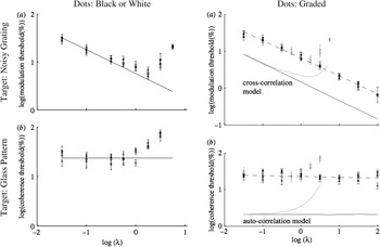
The prediction of FAQ (1) in Table 4 was tested by a psychophysical experiment whose results are shown in Fig. 1, from Barlow and Berry (Reference Barlow and Berry2011). Arrays of random dots can be given a streaky appearance by sinusoidal spatial modulation of the mean dot density to form a noisy sinusoidal grating whose distinctness increases with the depth of modulation, expressed here on double logarithmic coordinates as a percentage of the mean dot density at zero modulation. Observers report whether the streaks run top-left to bottom-right, or top-right to bottom-left, in many sample patterns with varying mean dot densities and %depths of modulation. Threshold was defined as the %modulation required to obtain D′ = 2 for correct discrimination and measured using a computer-controlled staircase method. Since the sequence of the trials was randomized, the observer never knew which of the many staircases was in use at any time. The results from three observers are the three U-shaped sets of data points in the top-left plot of Fig. 1.
.Human observers use both cross- and autocorrelation to detect orientational anisotropy in random dot displays. In these log/log plots, the experimental points are expected to lie on lines of slope −0.5 if cross-correlation is used, and 0.0 if autocorrelation is used, as explained in the text and in the original paper. When the anisotropy is produced by sinusoidal spatial modulation of mean dot density, as in the grating targets (upper pair), cross-correlation is used, but when it is generated by coherently oriented dot pairs, as in Glass patterns (lower pair), autocorrelation is used. The range of mean dot densities over which the relation holds is small—only about 30-fold for the left pair of plots,—but the pair on the right shows that this can be extended to 3000-fold by using graded dots to avoid the priority occlusion that becomes prominent in displays of binary (black or white) dots when the mean dot density approaches or exceeds 0.5 (see text). The thin lines without data points in the right-hand plots show the performance of computer models making ideal discriminations using cross-correlation (upper plots) or autocorrelation (lower plots) on the same dot patterns that were presented to the observers. They follow the forms of the psychophysical results very well, but the thresholds are lower. This figure is adapted from Barlow and Berry (Reference Barlow and Berry2011). For more details, consult text or original paper.

Oriented streakiness can also be produced by the procedure defined by Glass (Reference Glass1969). A fraction of the dots in a random dot pattern is given a companion dot displaced from it in a given direction and distance. If the directions of displacement are the same, and the separations subtend between about 6 and 10 min of arc at the observer’s eye, streakiness or “flow” is seen (Wilson & Wilkinson, Reference Wilson and Wilkinson1998). Again, thresholds for obtaining this effect can be measured by finding the minimum detectable percentage of coherently paired dots required for the appearance of flow; notice that a few such pairs will occur by chance, not by deliberate placement. The results are shown in the lower part of the figure. The coordinates are both logarithmic, using log(%amplitude modulation) and log(%coherence) as ordinates and log(mean dot density) as abscissa.
Using these coordinates, we expected the observers’ log(%modulation thresholds) for gratings, and log(%coherence thresholds) for Glass patterns, to be straight lines following the inverse square root relation (slope −0.5) with mean dot density in the first case and to be horizontal straight lines (slope 0.0) in the second case. These laws seem to hold well at low mean dot densities, but when the mean dot density is raised 30-fold and its log exceeds about −0.5 log(dots per pixel), both types of observed threshold are elevated more and more above their expected values.
We attribute this elevation to a well-known phenomenon we call “priority occlusion.” When using cells or pixels that are either black or white, as was the case in our first experiments, once a dot has been changed from black to white, it becomes insensitive to instructions to increase its luminance further, and obviously the threshold will rise. We therefore switched to using graded pixels, changing a line or two in our programs to delay the display, and first count the total number of dots programmed for each cell or pixel. The array was then displayed with each cell or pixel at a luminance proportional to the total number of dots programmed for that location. The displays then contain the information required for the eye to calculate cross- and autocorrelations correctly, averting priority occlusion, and it is clear from the results in Fig. 1 that it did so; now the expected laws are valid over ranges of mean dot densities above 3000-fold, instead of the 30-fold ranges when using binary (black or white) dots.
The lines without data points in the right-hand plots of Fig. 1 are computer simulations of ideal cross- and autocorrelators making threshold decisions on the same sets of test stimuli as those used for the psychophysical measurements. Notice that priority occlusion affects the simulations in the same way as it affects the psychophysical results; the strong implications of this result are mentioned later.
The good fit for the slopes using graded dots holds over very large ranges of mean dot density in both cases, but the fit does not hold for the absolute values of the thresholds. The psychophysical thresholds are higher than those for the simulations by a factor of about four for cross-correlations and about 12 for autocorrelation. The greater sensitivity of the simulations results largely from the fact that, being ideal detectors, their thresholds were calculated on the assumption that they combine information efficiently over the whole display area of the target, namely a circle of about 4° diameter. We cannot expect the real detectors to combine evidence with high efficiency over such large areas, partly no doubt because, if they did so, they would loose the information that enables them to localize the cross- or autocorrelated areas within the whole target area. We have found that, when the display area is reduced, all the thresholds are increased, but those for the simulations more than those of the psychophysical tests; consequently, the estimated psychophysical efficiencies are increased. We hope to consider elsewhere the highest attainable statistical efficiencies for psychophysical thresholds for these tasks.
Discussion
This is organized around four questions about the function and neural circuitry of the primary visual cortex of mammals and will be followed by stating the main conclusions and future outlook.
What are the main computational goals of the neural circuits in V1?
First, it is assumed that acquiring knowledge of the environment by appropriate statistical analysis of the sensory messages being received is a very important goal of sensory mechanisms in the visual cortex. Some are disconcerted by this approach and feel that it is obviously more important to pay attention to how the visual system responds to a “signal” than it is to analyze the unwanted responses to “noise.” The snag is that the difference between signal and noise is not necessarily known, so one is forced to study mixtures of them. There is no room for further justification of this approach, but the above snag may explain why the test signals used here are composed predominantly of randomly positioned dots, even though our real interest lies in detecting the small fraction of dots that follow some regularity or pattern.
Computational models are often tricky to interpret because the model contains unknown, or inaccurately known, parameters that leave plenty of room for spuriously improving the match between theory and experiment by making adjustments that cannot be justified by direct evidence. This is not a problem in the interpretation of Fig. 1. The two types of model considered here are very general, and probably should not be called “neural models” at all, but rather “possible computations.” They are: cross-correlation between a patch of the image and a fixed template, and spatial autocorrelation between two synchronous image patches. All the parameters of the detectors are determined by the requirement that they should be ideal for the purpose for which they are being used, and in our case, this means that they must be chosen to perform optimally for the parameters of the test stimuli that the observers were exposed to. These choices are based on first principles and cannot be adjusted arbitrarily to improve the match between theoretical predictions and experimental observations.
Another factor that strengthens our confidence in the significance of the differences in slopes of the experimental data in the right-hand pair of plots in Fig. 1, is the extraordinary range over which they hold. I think it is true that most psychophysical tests of theoretical predictions give results like those of the left pair of plots: the predictions hold, but only over a limited range of the variables concerned (here about 30-fold in mean dot density) and one is left with the awkward question: “Why do these laws not hold elsewhere?” We were lucky to be able to expand the ranges to about 3000-fold simply by avoiding priority occlusion. If standard programs for computing cross- or autocorrelations are run on images produced in this way, the computed thresholds will match those of psychophysical observers if their neural circuits also compute standard cross- or autocorrelations, and they will not match them if they do not. The results in the right half of Fig. 1 show that they do.
Notice also that the cross- and autocorrelation models were given the tasks of predicting the cross- or autocorrelation thresholds on the black/white dot patterns in which priority occlusion did occur, and these are shown by the curves for the models that have upward bends in them; the departures from predicted performances parallel those of the real system, and this surely strengthens one’s confidence that straightforward computations of cross- and autocorrelation are the appropriate ones for these neural circuits to perform.
What these results do not show is also important. They do not provide plausible neurophysiological models, simply because they do not deal with the variables one records in neurophysiological experiments on primary visual cortex. But the next step must be to find models that are neurophysiologically plausible, and it is surely true progress to have found two computations that account for observers’ thresholds over such large ranges.
Taking all the results shown in Fig. 1 together, I do not think one can avoid the conclusion that two distinct statistical mechanisms are available in early vision for detecting what can be termed “orientational anisotropies.” The noisy background of dots used in these experiments has dots positioned completely randomly over the whole target area, and completely independent of the positions of other dots. Orientational anisotropy was introduced either by making the mean dot density nonuniform over the target area, as we did with our noisy, spatially sinusoidal diagonal gratings, or by making the positions of some of the dots depend upon the positions of others, as we did by introducing coherently oriented diagonal dot pairs. The observers had no difficulty in responding to examples of either type of test target by signaling one of the three answers: “I see irregular streaks aligned bottom-left to top-right”; or “I see irregular streaks aligned bottom-right to top-left”; or “I am uncertain that it has either type of streak.” When the oriented streaks were well above threshold, the two types, produced either by modulating mean dot density or by introducing diagonally separated dot pairs, could be quite easily distinguished from each other, but this was not the case for streaks at threshold or just above it, and we did not ask for such distinctions to be attempted.
Hubel and Wiesel could not suspect that there were two different mechanisms for detecting orientational anisotropies when they claimed that the orientationally selective neurons in primary visual cortex could be divided into two classes, because Leon Glass only made his observations on moiré patterns in 1969, 10 years after Hubel and Wiesel had made the distinction between simple and complex cells. If they had known that orientational anisotropy is detectable by two different neural mechanisms, I feel sure they would have considered the possibility that simple cells use one mechanism, complex cells the other, and although it is a bit late in the day, I think we should now reexamine this possibility. Let us therefore cautiously consider the hypothesis that the simple cell/complex cell dichotomy is based on the cross-correlation/autocorrelation dichotomy: simple cells use cross-correlation, and complex cells use autocorrelation.
Missing neurophysiological evidence for autocorrelation
The strongest confirmation of the suggested role of complex cells would be to find that they are selectively sensitive to many different specific types of second-order associative structure in the input from the retina. Confining the tests to stationary stimuli, this would include stationary coherently organized dot pairs (as in Glass patterns), but with moving stimuli, it could include selectivity for colinear acceleration or deceleration, or for clockwise or anticlockwise changes in the direction of motion. Simple cells should obviously be tested in the same way, but they are not currently thought to be selective for such second- or higher-order associative characteristics of dot patterns: they are thought to be selective for a much smaller (but still large) number of first-order characteristics, depicted in random dot patterns solely by variations of mean dot density and not dependent at all upon relative positioning in pairs or larger groups of dots.
Neurophysiological efforts to sort this out may at first be thought superfluous because present methods are adequate for distinguishing complex from simple cells, but on the simplest form of the current hypothesis, one would expect the complex cells to belong to a much more heterogeneous group than the simple cells, simply because there are so many more types of second-order associative structure than there are types of simple first-order structure. If this is the case, we surely need to know it.
So far, when discussing cross- and autocorrelation, they have been considered as parallel operations, but Hubel and Wiesel thought that the inputs to complex cells came, mainly at least, from the simple cells. This suggests a serial model in which the second stage consists of a very large number of parallel autocorrelations between pairs of elements in the wavelet representation provided by the simple cells, selected from among the even vaster number of possible such pairs. The system could not possibly specify them all—there are far too many—so how does it restrict the choice to a limited number of suitable candidate pairs? How this is done is clearly a crucial question for such a model, which could not really be taken seriously without a suggested answer.
Fortunately, the answer seems obvious once one takes into account another important early result of the work of Hubel and Wiesel that has not so far even been mentioned: their discovery of cortical columns. Their evidence was based on determining the properties of single neurons recorded in succession at a large number of positions along a linear track through the cortex. From a large number of such tracks, they could find the rules governing the arrangements in three dimensions of neurons having particular orientational preferences and receptive field positions that were compatible with those they had actually found.
These and other experiments led them to conclude that the cortex has a columnar structure, with neurons having the same orientation preference arranged in columns normal to the cortical surface. This anatomical discovery points to a simple rule, based simply on propinquity, that might restrict what pairs of simple cells are tested for their joint activity, namely “Consider only pairs of simple cell inputs that lie close at hand in the same or neighboring columns, and at the same or similar depth from the cortical surface; exclude all others.”
Assigning a functional role to the columnar model of Hubel and Wiesel gives it a certain beauty and elegance, but an additional exclusion rule could have further functional significance. Consider a rule that says “If a potential autocorrelator detects too small a number of autocorrelations, disconnect one or both its inputs and try others.” Such a rule might, by selection, play a role in the actual formation of cortical columns; if not, it could at least improve the stability of the model by selective preservation.
A serial, cross-then-autocorrelation version of the hierarchical model of Hubel and Wiesel seems to be shaping up nicely, and we already know from Smith et al. (Reference Smith, Bair and Movshon2002) that cortical neurons are selective for the orientation of moving Glass-type patterns. Those experiments were not, however, designed to test whether autocorrelation was responsible, and they could usefully be extended in four ways:
• Stationary stimuli of about 160 ms duration should be used, since the type of autocorrelation contemplated works with stationary stimuli.
• The power spectrum of a Glass pattern is periodic, and to detect this with sufficient selectivity and statistical efficiency, one should probably use a receptive field that matches the whole periodic pattern, not just the single strongest frequency band in its power spectrum.
• To decide if the models perform well enough to explain behavioral results requires measurements of statistical efficiencies or another transferable measure.
• Priority occlusion should be avoided in order to increase the range of dot densities that can be used, as in the experiments of Fig. 1.
The missing background of psychophysical evidence
Before the experiments of Fig. 1 were done, we thought hard about tests that might depend on detecting either first-order statistical structure alone, or second-order statistical structure alone. The results show either that we thought and chose well, or were just lucky, but this needs to be followed up, for a large number of psychophysical questions in early vision suddenly present themselves, and it would be nice not to be alone in recognizing their importance. Can one detect motion either by autocorrelation or by cross-correlation, or both? How about autocorrelation in stereovision? Does it have a role in color? Is it specially important in coping with the effects of the unexpectedly large residual eye movements that have recently been described by Cherici et al. (Reference Cherici, Kuang, Poletti and Rucci2012) and Kuang et al. (Reference Kuang, Poletti, Victor and Rucci2012)?
It is clear that detecting Glass patterns requires the detection of a form of second-order associative structure, but we do not know if the second-order structure aids ordinary reading ability, or performance on the familiar Snellen test chart for acuity. Is it possible that detecting a second-order structure is more easily affected pathologically than detecting a first-order structure? What is its role in dyslexia or the visual problems of Alzheimer patients? Further investigations of the roles of first and second-order associative statistical structures are much needed and could be revealing in many ways.
Are plausible neuronal models for detecting autocorrelations within sight?
For the neural modeler, the main difficulty is likely to be that correlations can be of either sign, and any computation that can handle them easily should preferably use variables that can assume negative as well as positive values; but nerve cells communicate with each other chiefly by means of propagated all-or-none impulses, and there is no such thing as a negative number of impulses. Of course impulses can have inhibitory as well as excitatory effects, but knowing what we do about how synapses work, it is hard to imagine how linearity could be maintained across a synaptic junction simply by assigning negative numbers to inhibitory inputs: 10 excitatory impulses plus 10 inhibitory impulses are not expected to produce the same postsynaptic response as one (or none) of each.
One of the earliest discoveries about messages from the eye to the brain may provide the key to understanding how the brain resolves this difficulty: impulse frequencies in optic nerve fibers of vertebrates do not correspond to the illuminance of the parts of the retinal image they are connected to, but to the direction of change of illuminance in those parts, as shown by Hartline (Reference Hartline1938). It was later found (Barlow, Reference Barlow1953; Kuffler, Reference Kuffler1953) that change of spatial contrast, rather than change of illuminance, is what matters. Finally Heeger and his colleagues (Heeger, Reference Heeger1992; Carandini et al., Reference Carandini, Heeger and Movshon1997; Carandini & Heeger, Reference Carandini and Heeger2012) have shown that their nonlinear, threshold normalizing models predict well the responses actually generated by cortical neurons. Though it has not, to my knowledge, been done, Heeger-type models for computing both cross- and autocorrelation might be developed in which the ON and OFF systems are initially kept separate and only combined positively at the last moment. It is worth mentioning that some of the features of the model of the complex cell receptive field of Spitzer and Hochstein (Reference Spitzer and Hochstein1985) might fit such a model, though there are some discrepant features.
Conclusions
The main conclusions are that autocorrelation is the computation performed by the second level in the hierarchy Hubel and Wiesel proposed, that it is a much more powerful regularity-finding tool than cross-correlation alone, and that the columnar structure of the cortex, which Hubel and Wiesel also discovered, is an anatomical feature whereby pairs of inputs appropriate for the computation of autocorrelation could be selected by a simple rule. A scaffold constructed in this way would lead to the selection of pairs, just by their propinquity in the cortex, that would lead to them having receptive fields close to each other in the visual field, with similar optimal orientation selectivity, often coming from the same eye, though sometimes from different eyes. Such pairs are ones more likely to have substantial positive autocorrelations than the vast majority of all possible pairs that are remote from each other in the columnar-organized cortex, and thereby excluded by the suggested propinquity rule.
If different types of autocorrelation are performed in different parts of the cortex, these would, according to the scheme suggested here, result from differences in the columnar structure between different regions, for this is what determines the structure of the propinquities of different types of cortical neurons in the cortex itself, and this in turn determines what autocorrelations can and cannot be detected. This “structure of propinquities” would then play the part for autocorrelating cells that Hartline’s receptive fields play in determining what can be detected by cross-correlation, but it is not an altogether simple concept to grasp nor is it easy to see how to determine it experimentally.
These conclusions mean that we are closer to having a neurophysiologically plausible model of how the brain thinks than seemed likely only a few years ago, but note one final point: the conclusions do not follow from any prescriptive linking assumptions, but simply from the requirement (which has not yet actually been met, but I hope can be) that the computations postulated do their jobs as well as measures of behavioral performance show that the real brain can do them.
Future outlook
When the economist, Maynard Keynes, was sitting on an important government policy committee, the chairman is reputed to have taxed him with changing his opinion on some matter since the last meeting. “Well yes, I have,” Keynes replied, “but when the facts change, after due deliberation I do not hesitate to change my opinions. Pray tell me, sir, what do you recommend should be done in such circumstances?” After many years without much progress in understanding the functional significance of complex cells and cortical hierarchies, I think the facts have changed: the visual cortex uses autocorrelation as well as cross-correlation to detect and discriminate orientational anisotropies, and we now see that cortical columns may be an arrangement aiding the selection of suitable pairs for autocorrelation. We now need a nimble approach, perhaps more like that of Keynes than the one he suspected his chairman of following. If we take on board the importance of autocorrelation, and use computer simulations to test our theories intelligently, we may quite soon create models of how the brain thinks that are plausible at the neuronal level. In other words, we still do not know exactly how we think, but the answer is closer than many of us ever expected it to be.
Acknowledgments
The experimental work of fig 1 could not have been done without David Berry’s help, and the contents of Table 2 owes much to Mike Hawken. Graeme Mitchison, Dave Tolhurst, Tony Movshon, Eero Simoncelli and their colleagues at NYU have corrected some, but probably not all, of my misapprehensions about cortical neurophysiology and autocorrelation. The Department of Physiology, Development and Neuroscience in the University of Cambridge has provided space for experiments, and the Gatsby Foundation has provided welcome financial support for equipment and for Professor Berry’s visits, as has Trinity College. I have been helped by discussions about the brain with so many people over so many years that I cannot name you all, though I can and do thank you all.