1 Introduction
In the last two decades, feedback control of turbulent shear flows has become a grand challenge problem due to its important impact on technological applications (Brunton & Noack Reference Brunton and Noack2015). Closed-loop control has been shown to be necessary for changing operating conditions and can even improve on a working open-loop control at design conditions (King Reference King2010). Feedback controllers can reduce sensitivity to changing parameters in the system being controlled and to external perturbations, thus improving the robustness of the control (Aström & Murray Reference Aström and Murray2010). A plethora of model-based feedback control have been tested both numerically and experimentally with different flow configurations. For example, linear feedback control has been successfully employed in numerical studies to control the backward-facing step flow (Hervé et al. Reference Hervé, Sipp, Schmid and Samuelides2012) and the laminar flat plate boundary layer (Bagheri, Brandt & Henningson Reference Bagheri, Brandt and Henningson2009).
However, the application of closed-loop flow control to experiments dealing with transitional and turbulent flows focuses on slow variations of the operating conditions or in-time phasor control of oscillations. Indeed, physics-based linear models used by Rowley et al. (Reference Rowley, Williams, Colonius, Murray and Macmynowski2006) or Galerkin-based reduced-order models by Samimy et al. (Reference Samimy, Debiasi, Caraballo, Serrani, Yuan, Little and Myatt2007) led to effective closed-loop control of the cavity modes. Pastoor et al. (Reference Pastoor, Henning, Noack, King and Tadmor2008) achieved significant pressure drag reduction of bluff bodies using low-dimensional vortex models. Both the cavity and bluff body wake flows are dominated by an absolute instability and behave, therefore, as oscillators. Such oscillator flows are less sensitive to stochastic perturbations and their inherent global mode can be well identified for the purpose of control, as illustrated by the above-mentioned examples.
In contrast, free shear layers are dominated by convective instabilities and, therefore, behave as pure noise amplifiers. Consequently, each measurable property of the flow (characteristic frequencies, mixing layer thickness, etc.) continuously evolves along the streamwise direction and can only be interpreted locally. In addition, in case of a turbulent shear layer, the spatial evolution of dominant frequencies with respect to the locations of a sensor is the result of highly nonlinear mechanisms. The challenges are substantial for model-based control design in experiments (Cordier et al. Reference Cordier, Noack, Tissot, Lehnasch, Delville, Balajewicz, Daviller and Niven2013) and the flow control community frequently turns to model-free control methods.
Due to their conceptual simplicity, proportional–integral–derivative (PID) controllers were the first to be implemented. For example, Wiltse & Glezer (Reference Wiltse and Glezer2011) obtained a successful feedback control of the mixing rate in a fully developed mixing layer using a proportional–derivative (PD) controller. The feedback sensor was located just downstream of the splitter plate generating the mixing layer, and registered the initial Kelvin–Helmholtz (K–H) frequency of the flow. The PD control was then tuned to actuate in- or out-of-phase of the initial instability, and the effects on the mixing rate further downstream were explored. In Pinier et al. (Reference Pinier, Ausseur, Glauser and Higuchi2007), the proper orthogonal decomposition (POD) modes of the flow field of a separated shear layer were used as feedback information in order to reattach the flow to the surface of an airfoil. A mode which contained the relevant amplitude and frequency information was selected and a simple proportional control was applied to generate the actuation signal. Both of these cases required some tuning of the controller coefficients. In the former case, the control was locked at the natural frequency and the tuning was used to select the phase relationship, while in the latter, the frequency was given by a selection of the POD mode and the proportional control coefficient was tuned manually for an optimal amplitude response of the controller. Similar to Pinier et al. (Reference Pinier, Ausseur, Glauser and Higuchi2007), the POD mode feedback approach was successfully implemented in the control of a free shear layer by Parezanović et al. (Reference Parezanović, Laurentie, Fourment, Delville, Bonnet, Spohn, Duriez, Cordier, Noack and Abel2014). The POD modes of the unactuated flow which exhibited clear periodic behaviour were selected as the candidates for the feedback signal. This feedback approach modified the mixing layer by reinforcing flow synchronisation at the frequency of the selected POD mode, very similar to what is observed with periodic forcing at the same frequency.
These examples show that in the simplest cases the optimal parameters can be determined by a gradient search strategy. However, in more complex configurations, where multiple sensors and actuators of the plant are available, or when a specific objective should be achieved, it becomes hard to guess the appropriate parameters or feedback laws. In this case, the questions arise of how to automatically select the relevant flow sensors and how to automatically optimize the coefficients of the control law given a specific objective? One common way is to exploit the information contained in training data obtained by running the experiment with different control laws.
The question of inferring a function, here the feedback law, from training data can be reformulated as a symbolic regression problem. Symbolic regression extends classical regression techniques in the sense that no prespecified function structure is imposed in the identification. Instead, both model structure (analogous to selecting the best sensors or POD modes, and their combinations) and model parameters (analogous to tuning the coefficients of a PID controller) are sought. Since there is no assumption on the structure that best fits the data, symbolic regression is well suited to discover the hidden functional relationship between variables without the presence of a human expert. This relationship can be used to gain insight into the data-generating process and even to identify analytical laws that underlie physical phenomena in nature as in Schmidt & Lipson (Reference Schmidt and Lipson2009). Symbolic regression problems enter into the supervised learning subclass of the machine learning techniques (Murphy Reference Murphy2012). Genetic programming (GP), first introduced by Koza (Reference Koza1992) to train computers to solve problems without being explicitly programmed, is generally used for symbolic regression. GP belongs to the same family of evolutionary algorithms as the more familiar genetic algorithms (GA). Both techniques are biologically inspired heuristic optimization algorithms, imitating the process of natural evolution (Wahde Reference Wahde2008). An initial set of randomly created, suboptimal solutions undergoes an iterative process of improvement through genetic operations (elitism, replication, mutation and cross-over) in order to converge, after several generations, to the optimal solution. The optimization principles of evolutionary algorithms have been proved very successful in engineering problems such as aerodynamic shape optimization by Rechenberg (Reference Rechenberg1971). They are also well suited for turbulent flows and multiple-input, multiple-output (MIMO) control problems (Fleming & Purshouse Reference Fleming and Purshouse2002) since they can handle noisy objective functions and are easily implemented in optimization of multiple variables. Although GP and GA operate in a similar manner, they should not be confused. While for GP the search space corresponds to functions of variables, only parameters are optimized in GA. In that sense, GP can be interpreted as a generalization of GA. In the domain of flow control, Milano & Koumoutsakos (Reference Milano and Koumoutsakos2002) were among the first to use GA for the optimization of actuation parameters in order to minimize the drag of a cylinder. More general applications for system identification and control of nonlinear systems related to engineering applications can be found in Chang (Reference Chang2007).
In the case of a turbulent mixing layer, Parezanović et al. (Reference Parezanović, Laurentie, Fourment, Delville, Bonnet, Spohn, Duriez, Cordier, Noack and Abel2014) employed GP to determine the analytical expression for the best feedback control law, maximizing the turbulent kinetic energy. While the POD mode feedback approach relies on a specific selection of a particular POD mode, the GP process takes advantage of many sensor signals and their mutual phase and frequency differences to obtain an optimal closed-loop control law. The resulting closed-loop frequency was situated very close to the best open-loop frequency. Furthermore, due to the parameter optimization contained in the GP search process, the actuation signal became more periodic compared to the POD feedback. This type of closed-loop control has also been successfully applied by Gautier et al. (Reference Gautier, Aider, Duriez, Noack, Segond and Abel2015) in a single-input, single-output (SISO) experiment to minimize the recirculation zone of a backward-facing step.
This experimental study extends the preceding work implicating the use of closed-loop control in a turbulent mixing layer. The main objective is to explore what feedback frequencies can be established, when the control is based on sensors situated far downstream of the origin of a convective instability. In order to draw the most general conclusions, we decide to enlarge the solution space by using a model-free GP method for the design of the control laws. By analysing the actuated flow states, we aim to better understand the physical mechanisms which are exploited by the closed-loop control. This allows us to propose some general conditions for successfully establishing a feedback control in a convective mixing layer flow.
This paper is organized as follows. In § 2 we present the experimental set-up and outline the GP methodology. The performance and the robustness of the closed-loop control laws obtained by GP are evaluated in § 3. The composition of the control laws is analysed in § 4, to distil the main features of the optimization process performed by GP. In § 5 we discuss the physical mechanisms that are stimulated by forcing the mixing layer. Finally in § 6 the main findings are summarized and conclusions are drawn. In appendix A we give supplementary information on the influence of the streamwise position on the performance of both open- and closed-loop control, and the impact on feedback frequency selection. Appendix B details the GP procedure used in the experiments.
2 Experimental set-up and methodology
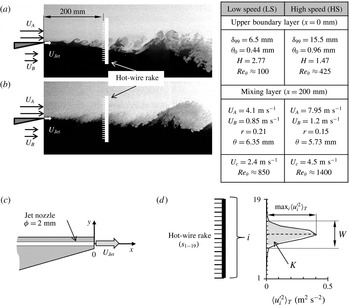
The mixing layer is created in a dual stream wind tunnel specifically designed for flow control. At the inlet of the test section, the wall between the two streams ends in a splitter plate, with a 3 mm thick trailing edge. Two speed configurations of the mixing layer are used: a low-speed (LS) configuration (figure 1
a) with a laminar upper boundary layer at separation, and a high-speed (HS) configuration (figure 1
b) featuring a turbulent upper boundary layer. The properties of these configurations and their upper boundary layers are given in the appropriate tables in figure 1. For characterizing the top boundary layer a single hot-wire probe was placed at the end of the splitter plate (
 $x=0$
) and displaced in the vertical
 $y$
direction in steps of 0.1 mm. The addition of a head loss device (foam) in the low-velocity stream reduced the maximum operational velocity for the lower stream in such a way that hot-wire measurements close to the lower boundary of the trailing edge were not sensitive enough. Additional information on the wind tunnel installation is available in Parezanović et al. (Reference Parezanović, Laurentie, Fourment, Delville, Bonnet, Spohn, Duriez, Cordier, Noack and Abel2014).
Mixing layer experiment. Visualization of the natural flow for: (a) LS and (b) HS configurations. (c) Close-up view of the splitter plate trailing edge and the actuator nozzle orientation. (d) Estimation of objective functions
 $W$
and
 $K$
using the velocity fluctuations profile.

The actuator system comprises 96 microvalves (MATRIX 820 Series) which pilot the opening of the 96 exit nozzles along the entire span of the trailing edge. The microjets produced by these nozzles are aligned with the horizontal
 $x$
axis to inject their momentum into the streamwise flow direction at the origin of the mixing layer (figure 1
c). Although the actuators are distributed discretely they are always activated unisonous, creating a continuous two-dimensional (2-D) spanwise disturbance. Since the actuators operate in a binary manner (open or closed), any input from the controller must be in a binary form. The highest frequency of actuation available to the microvalves is up to 800 Hz. The average amplitude of actuation is regulated by the pressure in the plenum chamber of the actuator system, which is kept constant. In this study, the average nozzle velocity of the jets was fixed to about
 $U_{jet}\approx 3~\text{m}~\text{s}^{-1}$
, which is of the same order of magnitude as the convective speed of the mixing layer. The actuation amplitude can be characterized by a mass flow rate coefficient
 $C_{q}={\dot{m}}_{a}/{\dot{m}}_{{\it\theta}}$
where
 ${\dot{m}}_{a}$
is the average mass flow rate of compressed air entering the plenum (measured by a Brooks 5863S mass flow meter) and
 ${\dot{m}}_{{\it\theta}}$
is the mean mass flow rate through the upper boundary layer.
With the exception of appendix A, where some results are presented at
 $x=500~\text{mm}$
from the origin of the mixing layer and the actuators, all the feedback experiments discussed in the text are done with the sensors placed at
 $x=200~\text{mm}$
. This distance corresponds to more than
 $450\times {\it\theta}_{0}$
, where
 ${\it\theta}_{0}$
is the momentum thickness of the upper stream boundary layer before detachment, for the LS configuration. The sensor system comprises a rake of 19 hot-wire probes, and furnishes both the feedback signals to the controller and the evaluation data for the objective function in the GP process. Discussion on the impact of the dual use of the sensors (both feedback and performance evaluation) is provided in appendix A.
The sensors are equally spaced every 8 mm and cover a vertical range between
 $-88~\text{mm}\leqslant y\leqslant +56~\text{mm}$
with respect to the trailing edge centre (
 $y=0$
). This is equivalent to almost five times the local vorticity thickness (
 ${\it\delta}_{{\it\omega}}\approx 30~\text{mm}$
) of the natural LS mixing layer as deduced from the hot-wire measurements. The downstream distance of the sensors implies a time delay which depends on the average convective velocity
 $U_{c}=(U_{A}+U_{B})/2$
, where
 $U_{A}$
and
 $U_{B}$
are the mean velocities of the upper and lower streams. The role of this convection effect in terms of frequency selection will be discussed in § 5.3. The reference values of
 $U_{c}$
and
 $Re_{{\it\theta}}$
for both mixing layer configurations in the self-similar region at
 $x=200~\text{mm}$
are also given in the tables in figure 1. Here, the local Reynolds number of the mixing layer is defined as
 $Re_{{\it\theta}}={\it\theta}U_{c}/{\it\nu}$
and the velocity ratio of the two streams as
 $r=U_{B}/U_{A}$
.
The hot-wire probes are of the classic single-wire design. Sensor signals used for feedback are acquired at a rate of 1 kHz, which corresponds also to the refresh rate of the real-time controller (Concurrent iHawk). The same sensor signals are simultaneously acquired by a second acquisition board at 5 kHz. These high-resolution data are used for a posteriori performance evaluation. The time delay caused by the controller hardware can be neglected compared with the dominant time scales of the flow configuration. In a plane turbulent mixing layer, the mean streamwise velocity is always larger than the two other mean velocity components. A wire perpendicular to the streamwise direction and aligned along the spanwise direction
 $z$
is then mainly sensitive to the streamwise component of the velocity (Bradshaw Reference Bradshaw1971; Delville Reference Delville1995). Hence, each sensor
 $i$
of the hot-wire rake measures the streamwise component of velocity. Fluctuations
 $u_{i}^{\prime }$
are obtained using the mean streamwise velocity
 $U_{i}$
averaged on a period of 2 s, which corresponds to around 180–240 K–H vortices (depending on the mixing layer speed configuration).
In this study, we use the so-called genetic programming control (GPC) framework to obtain optimal closed-loop control laws. This approach consists of using GP to determine the function of
 $n_{s}$
sensors
 $s_{i}$
(
 $i=1,\ldots ,n_{s}$
) which leads to a maximization of an imposed (arbitrary) objective function
 $J$
. Let
 $b(s_{i})$
be such a determined feedback control law, then the optimization is equivalent to the determination of a regression model
 $\mathscr{F}^{GP}$
such that
 $b(t)=\mathscr{F}^{GP}(s_{1}(t),\ldots ,s_{n_{s}}(t))$
for which
 $J$
is maximized. The closed-loop control laws obtained by GP are then continuous functions, based on the sensor signals as variables. However, the actuation system used in our experiments requires a binary command in order to operate. Therefore, the Heaviside function
 $\mathscr{H}$
must be applied to the control law
 $\mathscr{F}^{GP}$
, so that the actuation signal is given by
 $b(t)=\mathscr{H}(\mathscr{F}^{GP}(t))$
. As a consequence, all amplitude information in the control laws is lost, and there is an infinite number of control law expressions leading to the same actuation signal
 $b(t)=\mathscr{H}(\mathscr{F}^{GP})=\mathscr{H}({\it\lambda}\mathscr{F}^{GP})$
, for any
 ${\it\lambda}$
. With these considerations in mind, only the zero-crossings of the continuous functions
 $\mathscr{F}^{GP}$
are meaningful in terms of optimization. The decision of choosing GP to solve the symbolic regression problem was guided by the possibility of employing the same optimization algorithm independently of the actuators’ characteristics.
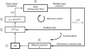
The control system schematically shown in figure 2 can be described as a multiple-input, single-output (MISO) system, considering that all actuators follow one control output
 $b(t)$
and we use multiple hot-wires as the sensor input
 $s_{i}=u_{i}^{\prime }$
.
Schematic representation of GPC framework in the experiment. The learning process starts with an initial set of randomly generated control laws
 $\mathscr{F}^{GP}$
 $\unicode[STIX]{x2460}$
. These are evaluated by the controller
 $\unicode[STIX]{x2461}$
using the real-time sensor signals
 $s_{i}$
as input. Since in our case, the actuator command of microjets is restricted to on/off signals, the controller output
 $\mathscr{F}^{GP}$
has to be binarized by the Heaviside function
 $\mathscr{H}$
 $\unicode[STIX]{x2462}$
before it can be used as actuation signal
 $b(t)$
. The flow data from the mixing layer plant
 $\unicode[STIX]{x2463}$
are recorded by the multiple sensors and sent back to the controller for continuous real-time evaluation of
 $\mathscr{F}^{GP}$
. The efficiency of the control law is estimated during the learning phase by computing the objective function
 $J$
 $\unicode[STIX]{x2464}$
. Based on the values of this objective function, the GP decides whether to keep, optimize or discard the tested control law. This learning process is repeated until the optimal control law is selected (subject to preimposed criteria). The learning phase is then completed and the controller continues to provide actuation based on the optimal control law and the real-time sensor data.

For the GP maximization, we consider two different objective functions defined as
 $$\begin{eqnarray}\displaystyle K=\mathop{\sum }_{i=1}^{n_{s}}\langle {u_{i}^{\prime }}^{2}(t)\rangle _{T}\quad \text{and}\quad W=\frac{2K}{\max _{i\in [1,n_{s}]}\langle {u_{i}^{\prime }}^{2}(t)\rangle _{T}}, & & \displaystyle\end{eqnarray}$$
where
 $n_{s}=19$
is the number of hot-wire probes and
 $T=10~\text{s}$
is the averaging time for obtaining velocity variances
 $\langle {u_{i}^{\prime }}^{2}\rangle _{T}$
. This averaging interval corresponds to a typical evaluation time of open-loop actuation or a closed-loop control law candidate. The objective function
 $K$
is proportional to an estimation of the turbulent kinetic energy in the mixing layer. The objective function
 $W$
is based on the local thickness of the mixing layer inferred from the velocity fluctuation profile shape, as represented on a sample profile shown in figure 1(d). The control effectiveness of both open-loop actuation and closed-loop control laws is presented in a non-dimensional form as
 $J_{K}=K/K_{u}$
and
 $J_{W}=W/W_{u}$
, where
 $K_{u}$
and
 $W_{u}$
are reference values of the objective functions for the unactuated mixing layer. Using all 19 hot-wires improves the resolution of the velocity fluctuations profiles and, therefore, the estimation of the objective function. To simplify the optimization problem, only every third hot-wire is available for the GP learning process. Hence, only the sensors
 $s_{1}$
,
 $s_{4}$
,
 $s_{7}$
,
 $s_{10}$
,
 $s_{13}$
,
 $s_{16}$
and
 $s_{19}$
can be used as variables by the GP, in any control law. Preliminary test showed that the spectral content of these sensors gives a good representation of the variety of physical scales present at a given streamwise location in the mixing layer.
The GP learning phase is completed by reaching either the imposed criterion on the value of the objective function, or the predetermined final generation of individuals. The best performing individual of the final generation is selected as the closed-loop control law, and the GP module is disconnected to engage autonomous real-time control. The specific aspects of implementing GPC in the mixing layer experiment are discussed in appendix B. Further details on the GPC framework can be found in Duriez et al. (Reference Duriez, Parezanović, Laurentie, Fourment, Delville, Bonnet, Cordier, Noack, Segond and Abel2014).
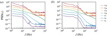
PSD of the selected hot-wire sensors of the unactuated mixing layer at
 $x=200~\text{mm}$
, for (a)
 $Re_{{\it\theta}}=850$
(LS) and (b)
 $Re_{{\it\theta}}=1400$
(HS) flow speed configurations. The PSD plots are in log–log scale with amplitudes offset by a decade, for clarity. The dashed line corresponds to a Strouhal number
 $St_{{\it\theta}}\approx 0.032$
.

3 Closed-loop control performance
In this section we evaluate the impact of the GP-optimized control laws on the mixing layer. We first characterize the spectral content of the unactuated baseline flow, in § 3.1. The performance of the best closed-loop control laws is compared with the reference open-loop forcing, in § 3.2. Finally, in § 3.3, we test the robustness of both open- and closed-loop control, with respect to the changes of the free-stream velocities.
3.1 The unactuated mixing layer
Analysing the temporal evolution of the different hot-wire signals at
 $x=200~\text{mm}$
provides indications on the naturally present frequencies at this location. Figure 3 shows the power spectral density (PSD) of each sensor signal (used in closed-loop control) for the two flow configurations. With the exception of the sensor signals at the centre of the mixing layer,
 $s_{10}$
and
 $s_{13}$
, all the spectra of the sensors show a distinct local maximum. In accordance with previous findings of Winant & Browand (Reference Winant and Browand1974) and Morris & Foss (Reference Morris and Foss2003), this ‘hump’ points to the existence of a preferred mode of the flow, which occupies a narrow band of frequencies. Following Ho & Huerre (Reference Ho and Huerre1984), the natural Strouhal number in a laminar mixing layer is
 $St_{{\it\theta}}=(f_{n}{\it\theta})/U_{c}=0.032$
, where
 ${\it\theta}$
is the local momentum thickness. The frequencies corresponding to this Strouhal number are estimated using the values of
 ${\it\theta}$
and
 $U_{c}$
given in the tables of figure 1. The estimation yields 12 and 25 Hz for the LS and HS configurations, respectively. As indicated in figure 3, these values are well inside the frequency range of the humps, visible in the spectra of the sensors outside the centre of the mixing layer. Hot-wire sensors
 $s_{10}$
and
 $s_{13}$
, close to the centre of the mixing layer are less sensitive to vortex shedding due to a vanishing mean value of the vertical velocity component. For comparison, the PSD measured near the trailing edge of the splitter plate at
 $x=50~\text{mm}$
(not shown here) feature much more clearly defined peaks around 90 Hz (LS) and 120 Hz (HS). These higher frequencies are related to the K–H instability caused by the boundary conditions imposed at the trailing edge of the splitter plate (Morris & Foss Reference Morris and Foss2003). The lower frequencies measured at
 $x=200~\text{mm}$
(shown in figure 3) correspond to the amplifier dynamics of the mixing layer in the self-similarity region, which is no longer influenced by the local formation conditions of the shear layer.
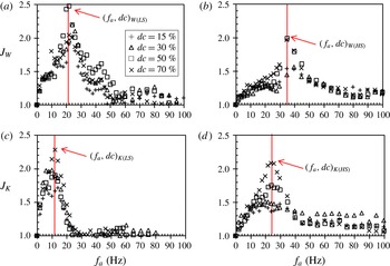
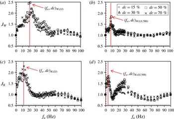
Mapping of objective functions
 $J_{W}$
and
 $J_{K}$
, for a range of open-loop actuation frequencies
 $0~\text{Hz}<f_{a}<100~\text{Hz}$
, and four different duty cycles (15 %, 30 %, 50 %, 70 %), in (a,c)
 $Re_{{\it\theta}}=850$
(LS) and (b,d)
 $Re_{{\it\theta}}=1400$
(HS) configurations of the mixing layer (sensors located at
 $x=200~\text{mm}$
). Red vertical line (colour online only) in each case represents the obtained frequency and the associated duty cycle of open-loop control for which the corresponding objective function is maximized. These values are noted as value pairs (
 $f_{a},dc$
) in the text, for each case.

3.2 Periodic forcing and closed-loop control
In order to set a reference for the closed-loop control, the mixing layer response to periodic forcing has been mapped for the entire range of available actuation frequencies (
 $f_{a}$
), up to 500 Hz and for several values of duty cycles (
 $dc$
). The mapping results for the LS and HS configurations are shown in further text up to
 $f_{a}=100~\text{Hz}$
, since this is the most interesting actuation range with respect to the defined objective functions.
From the open-loop mapping we find the optimal settings of
 $(f_{a},dc)_{W(LS)}=(21~\text{Hz},50\,\%)$
for maximization of the objective function
 $J_{W}$
in the LS configuration (figure 4
a). The maximum of
 $J_{K}$
is obtained for
 $(f_{a},dc)_{K(LS)}=(12~\text{Hz},70\,\%)$
(figure 4
c). The open-loop mapping experiment in the HS configuration of the mixing layer is shown in the right column of the figure 4. In the this configuration, open-loop mapping yields
 $(f,dc)_{W(HS)}=(35~\text{Hz},50\,\%)$
as the best periodic actuation parameter pair for the maximization of
 $J_{W}$
(figure 4
b), and
 $(f_{a},dc)_{K(HS)}=(24~\text{Hz},70\,\%)$
for the maximization of
 $J_{K}$
(figure 4
d).
We can conclude that the two objective functions are maximized for two different actuation frequencies. Also, the mapping experiments in LS and HS configurations show that the optimal actuation frequency depends on the free-stream velocities of the mixing layer. In both mixing layer configurations, the objective function
 $J_{K}$
is maximized when the actuation frequencies are around the estimated local natural frequency. Objective function
 $J_{W}$
reaches a maximum when the actuation is performed around 1.45–1.75 times the optimal frequency for
 $J_{K}$
.
The duty cycle of actuation apparently plays a significant role only around the actuation frequency where a given objective function is maximized. This means that by choosing an arbitrary objective function, we may not see the effect of the duty cycle outside of the actuation range corresponding to the optimal parameters for this objective function.
These results show that a maximization of an arbitrary objective function might require a frequency of actuation which is not necessarily the local natural frequency, nor its multiple. Such an actuation frequency can be easily imposed by an open-loop control, but the question is: can we build a closed-loop controller which will be able to find and use such frequency automatically, taking into account that such a hypothetical frequency may not be a dominant natural mode?
The GP search process has been performed for the maximization of the two objective functions
 $J_{W}$
and
 $J_{K}$
, yielding control laws
 $\mathscr{F}_{W(LS)}^{GP}$
and
 $\mathscr{F}_{K(LS)}^{GP}$
for the LS mixing layer configuration:
 $$\begin{eqnarray}\displaystyle \mathscr{F}_{W(LS)}^{GP}=\sin (\exp (s_{19}\times \exp (s_{1}^{2})-s_{16})-\cos (\exp (s_{13})\times s_{1}^{2}\times s_{19}\times s_{16})) & & \displaystyle\end{eqnarray}$$
and
 $$\begin{eqnarray}\displaystyle \mathscr{F}_{K(LS)}^{GP}=s_{19}+s_{19}+\sin (\sin (\sin (\sin (s_{16}-s_{1})))). & & \displaystyle\end{eqnarray}$$
The index
 $K$
or
 $W$
denotes that the control law
 $\mathscr{F}^{GP}$
is the optimal solution for the maximization of the respective objective function. Index (LS) or (HS) indicates in which flow configuration has the control law been trained by the GP.
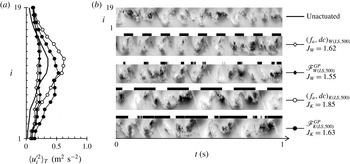
Resulting
 $\langle {u_{i}^{\prime }}^{2}\rangle _{T}$
profiles (a) and pseudovisualizations (b) for maximization of
 $J_{W}$
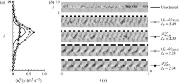
and
 $J_{K}$
experiments in LS configuration of the mixing layer. The best open- and closed-loop control are compared. Actuator system input is marked using black and white stripes above each case (black stands for active). The pseudovisualizations are constructed from
 $u_{i}^{\prime }$
in a range of
 $-1.5$
to
 $1.5~(\text{m}~\text{s}^{-1})$
and are based on Taylor’s hypothesis of frozen turbulence.

The results of both open- and closed-loop control on the velocity fluctuation profiles can be seen in figure 5(a). When maximizing the cost function
 $J_{W}$
, the resulting fluctuation profiles are a near match for both controls. However, their shape is significantly different compared to the natural flow; we observe a larger spread of fluctuations across the mixing layer and a lower maximum amplitude around the middle. Maximization of
 $J_{K}$
leads to an increase in fluctuation amplitude across the entire profile, while the general shape is similar to the natural case.
Figure 5(b) shows the pseudovisualizations of the natural LS flow, followed by open- and closed-loop control cases for the two objective functions. The closed-loop control laws
 $\mathscr{F}_{W(LS)}^{GP}$
and
 $\mathscr{F}_{K(LS)}^{GP}$
feature almost perfectly periodic actuation, although time is not an explicit variable in the control laws. Clearly, in both cases, the feedback control has caused a resonance close to the specific frequency which was found the most effective for open-loop control; around 20 Hz for
 $J_{W}$
and around
 $12~\text{Hz}$
for
 $J_{K}$
. The actuation stripes in figure 5(b) indicate that the duty cycles are also similar to the open-loop reference case. Corresponding pseudovisualizations reveal that the mixing layer flow is well ordered on the scales of actuation. The cost function values of open- and closed-loop control are comparable to within 5 %.
The whole process of the GP search for the best control law was repeated five times for each of the objective functions, and in all cases the control laws produced identical frequency selection. The resulting values of the objective function were reproducible for any given control law. The standard deviation of the maximum values of both objective functions, measured over all experiments (typically more than 20 evaluations), lies in the range
 $0.08<J_{rms}<0.2$
for both open- and closed-loop control.
3.3 Robustness of closed-loop control
In this section, we test and compare the robustness of both open- and closed-loop control strategies with respect to changes of the mixing layer stream velocities. The best solutions presented in § 3.2 for the closed-loop control have been trained by the GP in the LS mixing layer configuration. Using the GP search, we find the best closed-loop control law optimized specifically for the HS configuration:
 $$\begin{eqnarray}\displaystyle \mathscr{F}_{W(HS)}^{GP}=s_{7}\times \exp (s_{4}-s_{1})+s_{4}. & & \displaystyle\end{eqnarray}$$
For this control law, as well as for the open-loop actuation
 $(f,dc)_{W(HS)}=$
(
 $35~\text{Hz}$
, 50 %), the HS configuration of the mixing layer is the design point. To test their robustness, we apply both of them to off-design conditions. For this purpose, the LS configuration, studied in more detail in the previous section, is selected as the off-design condition. We emphasize that the HS design condition comprises a fully turbulent mixing layer, from the onset. The off-design LS configuration with a laminar origin of the mixing layer is therefore the most different flow configuration available in our experiments, without significantly changing stream velocity ratio
 $r$
. Other stream velocities between the LS and HS configurations represent comparatively minor modifications of the flow conditions.
Comparative tests of the best open-loop actuation
 $(f_{a},dc)_{W(HS)}$
and the best closed-loop control law
 $\mathscr{F}_{W(HS)}^{GP}$
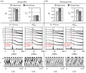
applied at the design point HS and the off-design point LS. In the upper row, the objective function
 $J_{W}$
and the corresponding mass flow rate coefficient
 $C_{q}$
values are represented. In the middle row, the PSD of every third hot-wire probe are shown in log–log scale, shifted by a decade for clarity. The PSD of the binary actuation signal is shown in a linear-log scale in the bottom of each window (line ‘b’). In the lower row, pseudovisualizations are shown on a time duration of
 $t=0.25~\text{s}$
. The associated grey-scale map depicts
 $u^{\prime }$
in a range of
 $-1.5$
to
 $1.5~(\text{m}~\text{s}^{-1})$
. Black and white stripes depict the associated actuation (black for active).

Figure 6 compares best open- and closed-loop control when applied to (a) design and (b) off-design flow conditions. The values of the objective function
 $J_{W}$
and the actuation cost
 $C_{q}$
are comparable for the two controls in the design case (bar diagrams in figure 6
a), with a slight advantage for the open loop. However, the corresponding diagrams in the LS off-design case (figure 6
b) show a drastic decrease in performance when the open-loop actuation for the HS configuration is applied, while the best closed-loop control for HS maintains its effectiveness.
Under design conditions the spectral analysis shown in figure 6(a) shows for both types of control the fluctuation energy concentrated around the actuation frequency. In figure 6(b) when the best HS closed-loop control law
 $\mathscr{F}_{W(HS)}^{GP}$
is applied under the LS off-design conditions, the closed-loop control selects the correct optimal actuation frequency and synchronizes the mixing layer in a similar way as in figure 5. Furthermore, when the best HS open-loop
 $(f_{a},dc)_{W(HS)}$
is applied in the off-design case (LS), we observe a significant reduction in the energy content at the actuation frequency. In the LS mixing layer, the frequency of
 $35~\text{Hz}$
no longer corresponds to the optimal frequency, and the pseudovisualization reveals only weakly defined structures inside the mixing layer. The closed-loop control adapted itself to a nearly periodic 21 Hz actuation regime, in agreement with the optimal open-loop control for this flow configuration. Although the spectra for this case show other frequencies present, the most energetic peak is at this optimal frequency, and appears to be as well amplified as in the design case. The corresponding imposed periodic structures inside the mixing layer, visible in the pseudovisualization are very similar to the optimum for the LS case (see figure 5
b).
For these off-design conditions, the comparison between open- and closed-loop control clearly favours the closed loop. The reference control for the LS configuration is the optimal open-loop actuation
 $(f_{a},dc)_{W(LS)}$
, which achieves
 $J_{W}=2.49$
(see figure 4
a). Using the optimal HS actuation
 $(f_{a},dc)_{W(HS)}$
in the LS off-design configuration results in
 $J_{W}=1.4$
. This is a reduction of
 $44\,\%$
with respect to the reference objective function value. The closed-loop control
 $\mathscr{F}_{W(HS)}^{GP}$
adapts to off-design conditions much more efficiently: objective function value of
 $J_{W}=1.91$
is obtained, yielding only 22 % of reduction in effectiveness compared with the reference value. A reverse robustness test reveals similar results, when optimal closed- and open-loop actuation signals for the LS case are applied to the HS configuration as the off-design condition.
A priori, closed-loop control can perform either better or worse than the open-loop control in design and off-design conditions. Here, the robustness property of the GP process can be partially attributed (see the survey of Beyer & Sendhoff (Reference Beyer and Sendhoff2007)) to the stochastic nature of evolutionary algorithms for which the optimal solution is obtained after many generations of evolution by operating on a large population of potential solutions. In § 5.1, we propose another explanation of this particular robustness result based on the anatomy of the best control laws found by GP in the HS configuration (§ 4.1) and on the frequency response to periodic forcing at the sensor location. It may be noted that like in
 $\mathscr{H}_{\infty }$
-control problems (Burl Reference Burl1999), GP can, in principle, take into account the robustness to external perturbations if the operating conditions are taken into consideration in the cost function during the learning phase. In addition, GP can combine periodic forcing and sensor feedback or even choose between open- and closed-loop control, depending on which performs better. These generalizations shall be part of future publications.
4 Analysis of closed-loop control laws
In § 4.1, the best control laws obtained by GP are analysed in detail in order to provide more understanding of how a specific feedback frequency is obtained. In § 4.2, we show that closed-loop control laws exist, which synchronize the mixing layer at frequencies other than optimal frequencies for the maximization of the imposed objective functions. In § 4.3, we discuss the observed periodicity of the feedback control and propose mechanisms which could enable it.
4.1 The anatomy of the best control laws
The probabilistic manner in which the GP constructs and manipulates the expressions of the control laws (see appendix B) means that there may be multiple control laws with different analytical expressions, but which perform the same action. For example, we can consider a simple hypothetical situation where two control laws
 $\mathscr{F}_{n}^{GP}=s_{19}$
and
 $\mathscr{F}_{m}^{GP}=s_{19}+s_{1}-s_{1}$
are produced during the GP process. At a first glance we can immediately acknowledge that these two control laws are identical, but the GP process treats them as different individuals. In addition to this, the actuator system design requires that the Heaviside function is applied on the control law (see § 2), which is another reason why control laws of different analytical expressions may produce a similar result
 $b(t)$
.
With this in mind, an efficient way to classify the solutions obtained by GP is to compare the spectra of the actuation signals
 $b(t)$
. If the actuation spectra of two control laws match, we consider that the two control laws are equivalent, regardless of their analytical expressions. The matching is computed as a linear correlation coefficient
 $r_{c}$
between spectral amplitudes and needs to be better than
 $r_{c}\geqslant 0.95$
. If we examine the analytical expressions of control laws matched in this way, we can obtain a statistical image of participation of different sensors in their expressions. Only a single occurrence of any given sensor is counted, regardless of how many times this sensor was repeated in the control law expression. A histogram is then computed with bins corresponding to the different sensor labels
 $s_{i}$
.
We consider the best HS control law
 $\mathscr{F}_{W(HS)}^{GP}$
(3.3) as reference for the matching of actuation spectra. The reference spectrum of the control law actuation signal PSD(
 $b$
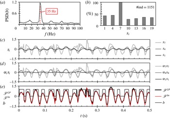
) is shown in figure 7(a). The search for equivalent control laws yields 1151 matches of the actuation spectrum within the whole GP experiment. The histogram of the participating sensors, in the control laws acting similarly as
 $\mathscr{F}_{W(HS)}^{GP}$
, is shown in figure 7(b). We can see that sensor
 $s_{7}$
is present
 $100\,\%$
of the time, while other sensors appear less often in relatively equal proportions. We can conjecture that this sensor is necessary to enable a nearly periodic actuation at 35 Hz. But do the remaining sensors play a role, or are they just artefacts of the GP optimization process?
Analysis of the best control law
 $\mathscr{F}_{W(HS)}^{GP}$
: (a) power spectral density of the square wave actuation signal
 $b_{W(HS)}(t)$
, (b) histogram of sensor occurrence in all individuals matching the actuation spectra of
 $\mathscr{F}_{W(HS)}^{GP}$
, (c) recorded sensor signals
 $s_{i}$
, (d) sensor signals with linear regression weighting applied (
 ${\it\alpha}_{i}s_{i}$
) and (e) linear regression reconstruction corresponding to
 $\mathscr{F}_{W(HS)}^{lin}=-0.34\times s_{1}+1.266\times s_{4}+0.943\times s_{7}$
, plotted for comparison with
 $\mathscr{F}_{W(HS)}^{GP}$
and
 $b_{W(HS)}(t)$
for reference. Label #ind indicates the number of individuals matching the reference actuation spectrum.

It turns out that the best control laws obtained by GP (3.1)–(3.3) can all be represented by a linear expression. We have used linear regression to reconstruct the actuation signal
 $b(t)$
by representing the control laws as a linear combination of the sensors
 $s_{i}$
, with associated weighting coefficients
 ${\it\alpha}_{i}$
. This is further illustrated in figure 7(c–e) for the HS configuration. The three hot-wire sensors used (
 $s_{1}$
,
 $s_{4}$
and
 $s_{7}$
) are all located on the lower part of the sensor rake, inside the low-velocity region of the mixing layer. As shown in figure 7(c), the closer the sensor is to the centre of the mixing layer, the larger are the recorded velocity fluctuations. All these data were obtained for the actuated state and all three sensors show fluctuations principally caused by actuation. However, significant differences exist between each of the signals; sensor
 $s_{7}$
recorded a much noisier signal than the other two. The transient events observed in this signal appear to be stochastic perturbations caused by the evolution of small-scale structures inside the core of the mixing layer. Nevertheless, the linear regression weighting shown in figure 7(d) further highlights that sensor
 $s_{7}$
represents the main sensor input, in accordance with its domination in the histogram 7(b). Here
 $s_{4}$
is scaled up to roughly the same amplitude level as
 $s_{7}$
but
 $s_{1}$
is significantly reduced. The corresponding linear approximation of the control law
 $\mathscr{F}_{W(HS)}^{lin}$
in figure 7(e) suggests that the dominant (but noisy) signal of
 $s_{7}$
is smoothed out by its combination with
 $s_{4}$
.
The apparently non-essential sensors contribute to the efficiency of a control law by a modification of the duty cycle. As shown in figure 4, the objective functions are highly sensitive to the values of the duty cycle around the optimal open-loop parameters. In our experiment, the duty cycle is the only way to modify the amplitude of actuation, taking into account that the actuator system works with a fixed level of pressure, and that the Heaviside function must be applied to binarize the control signal. If we use only a single weighted sensor signal
 ${\it\alpha}_{i}s_{i}$
at a time, for the linear approximation, we can estimate what duty cycle would each sensor produce. The results for
 $\mathscr{F}_{W(HS)}^{lin}$
are:
 $48\,\%$
using
 $s_{1}$
,
 $54\,\%$
with
 $s_{4}$
and
 $60\,\%$
with
 $s_{7}$
only. The measured duty cycle of this control law is
 $55\,\%$
.
This implies that combining the signals contributes to the optimization of the duty cycle. However, there is no reason why scaling the ‘dominant’ sensor signal with an appropriate constant generated randomly by GP could not perform the same task. Genetic programming can generate random constants in a range of
 $-1.00$
to 1.00 (see appendix B), but in our experience, the GP seems to be more efficient in using other variables as scaling instead of constants. Moreover, from the histogram of the sensor participation in this control law, it appears that all of the other ‘supporting’ sensors can be used equally often, and that there is no obvious pattern for their selection. Therefore, in the case of
 $\mathscr{F}_{W(HS)}^{GP}$
, the use of other sensors can be considered as an idiosyncrasy of genetic programming.
The control laws
 $\mathscr{F}_{W(LS)}^{GP}$
(3.1) and
 $\mathscr{F}_{K(LS)}^{GP}$
(3.2), which are trained to maximize the two objective functions in the LS flow configuration, similarly have a single sensor which is always present in the control law expression. In the case of
 $\mathscr{F}_{W(LS)}^{GP}$
, only the sensor
 $s_{16}$
appears all the time, and the flow is synchronized around
 $20~\text{Hz}$
in the LS configuration. For
 $\mathscr{F}_{K(LS)}^{GP}$
, the dominant sensor is
 $s_{19}$
which produces synchronization around
 $12~\text{Hz}$
. We will further discuss some aspects of the vertical location of the dominant sensor in § 5.3.
4.2 Diversity of the feedback frequency selection
The chosen objective functions
 $J_{K}$
and
 $J_{W}$
are arbitrary, but physics based. Each is maximized by causing a lock-on state of the mixing layer at a different optimal frequency. The GP successfully designed closed-loop control laws which are based on those frequencies (see § 3.3). If the feedback control can be designed to use these two frequencies, can we then expect that there are other frequencies, on which the feedback can be established?
The GP process, in its learning phase, creates a multitude of control law individuals which are discarded because they do not maximize the imposed objective function. This does not mean, however, that all of them are meaningless and that such control laws would not maximize some other arbitrary objective function. The results in § 3 suggest that the most efficient control laws produce near-periodic actuation. In these cases, the spectrum of the actuation signal features a well-defined energy peak around a single frequency. If the spectrum of actuation features a badly defined peak or a broadband energy distribution, such a control law usually performs badly. In the experiments performed, non-periodic or stochastic actuation does not appear to produce any remarkable effects within the observed portion of the mixing layer. We therefore assume that any existing alternative solution of the feedback control will feature a nearly periodic actuation signal based on a frequency, other than what was observed so far. The control laws deemed as suboptimal and discarded by the GP process, can provide a large sample base in which alternative synchronized states of the mixing layer might be found. Instead of designing many new objective functions which would enable us to find these alternative solutions, we can simply browse through the already existing, but apparently suboptimal solutions.
After a short search through all the individuals produced within one GP experiment in the HS mixing layer configuration, we can find at least five control laws which feature an actuation spectrum with a well-defined peak around a suboptimal frequency (with respect to
 $J_{W}$
). The matching of the actuation spectra (as in the § 4.1) allows us to discover all of the individuals which produce these alternative actuation spectra, and to analyse the sensor participation histograms. Since these control laws do not maximize
 $J_{W}$
, we identify them using the number of the individual, in the first generation of the experiment, for which this type of actuation spectrum has been first observed.
Examples of suboptimal control laws found in the GP experiment for the maximization of
 $W$
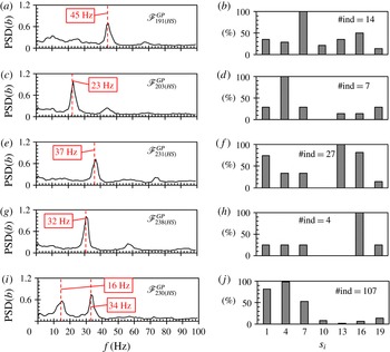
in HS mixing layer configuration. Shown on the left are power spectral densities of different actuation signals
 $b(t)$
used for the matching analysis. The corresponding histograms of occurrence of specific sensors are shown on the right. The numbering in the control law name denotes the number of the individual in the first generation of the experiment. Label #ind indicates the number of individuals matching the reference actuation spectrum.

The actuation spectra of these alternative solutions are shown in figure 8, with their associated histograms of sensor participation. Of particular interest is the case (figure 8
a,b) where the control law
 $\mathscr{F}_{191(HS)}^{GP}$
provokes a well-defined actuation at
 $45~\text{Hz}$
. From its histogram, it appears that the hot-wire
 $s_{7}$
(same as in
 $\mathscr{F}_{W(HS)}^{GP}$
discussed earlier in § 4.1) is the only essential sensor. It follows that the selection of a dominant sensor is not the only condition to obtain a given feedback frequency. The scaling in the control law or the combination with another sensor(s) also plays an important part in determining the behaviour of the solution. The control law
 $\mathscr{F}_{203(HS)}^{GP}$
(figure 8
c,d) selects 23 Hz as the dominant actuation frequency, which is very close to the open-loop frequency which maximizes
 $J_{K}$
in the HS configuration (see figure 4
d). We have not performed a dedicated GP search to maximize
 $J_{K}$
in the HS flow, but this individual appears as a candidate to fulfil this objective. The other solutions found include well-defined peaks at actuation frequencies very close, yet distinctly different from the optimal actuation (35 Hz) for maximizing
 $W$
:
 $\mathscr{F}_{231(HS)}^{GP}$
37 Hz (figure 8
e,f) and
 $\mathscr{F}_{238(HS)}^{GP}$
32 Hz (figure 8
g,h). This confirms that an automatic selection of the sensor and an optimized scaling of the signal(s) within the control law can tune a mixing layer synchronisation frequency with high precision.
Finally, in spite of the MISO design of the control system in this experiment, and the ability to impose only a single actuation frequency in the open-loop case, the closed-loop control
 $\mathscr{F}_{230(HS)}^{GP}$
might even be able to produce some kind of frequency cross-talk effect, as evidenced in the spectra in figure 8(i,j), where two well-defined peaks can be observed. Here, the first peak is a low-frequency modulation of the actuation frequency based around the second peak. This case, however, does not appear in sufficient number of samples to provide a solid base for further discussion of the dynamics involved. Finally, all of these examples represent control laws either created randomly in the first GP generation or created by modification of later individuals by random mutations. This means that they have not undergone the optimization process and might still be improved if an objective function would target them.
4.3 The periodicity of feedback control
The linear approximation of the GP control law expression has been performed using the data from the actuated flow, i.e. where the controlled state of the mixing layer is fully established. Hence, the synchronization mechanism found by GP greatly simplifies the dynamics of the actuated mixing layer in comparison to the natural flow, presented in § 3.1. For both open- and closed-loop control, the input frequency of the actuation system was recovered by the sensor system, as shown in the spectra in figure 6. It seems therefore that this phenomenon called the lock-on flow in the literature (Baek & Sung Reference Baek and Sung2000) is a crucial lead for understanding the potential capabilities of the frequency selection by the feedback control. In our experiments, the amplitude of actuation is large and the energy of perturbations inserted into the mixing layer is of the same order of magnitude as the energy of the unactuated flow (
 $U_{jet}\approx U_{c}$
). In this case it is expected (Oster & Wygnanski Reference Oster and Wygnanski1982; Fiedler & Mensing Reference Fiedler and Mensing1985) that the mixing layer will be well organized at the frequency of actuation in the streamwise region where these perturbations are amplified (see also figure 9).
For closed-loop control this means that once the first perturbation created by the actuators reaches the sensor array, every consequent cycle of actuation might be triggered by the perturbations created by one of the previous cycles. This is also the reason, why the observed closed-loop actuation becomes so periodic; establishing a controlled state means triggering a perturbation of specific properties. The controller then just acts on the perturbation and the cycle is self-repeating. Therefore, the basic requirement is that the perturbation created by actuation is amplified sufficiently to be captured by the sensor array. Here, the well-known mechanism of wave amplification by a shear flow (Michalke Reference Michalke1965; Ho & Huerre Reference Ho and Huerre1984) contributes to the determination of which types of perturbations can be used for feedback synchronization at a given location of the sensor array.
Nonlinear mechanisms present in the turbulent mixing layer can sometimes affect a cycle in unpredicted ways. This is why the closed-loop control can never be as periodic as the open-loop, i.e. the next cycle depends on how the previous cycle was registered by the sensors. Clearly, the control law must be designed in such a way as to minimize the negative effects of random flow perturbations on the repeated creation of an optimal actuation pulse.
5 Physical mechanisms in the forced mixing layer
We have previously proposed that a perturbation created by actuation needs to be amplified by the mixing layer in order to cause a successful self-repeating cycle. In § 5.1, we examine, based on open-loop actuation, what types of perturbations can potentially fulfil this condition. In § 5.2, we explore different physical mechanisms that can be observed in the actuated mixing layer flow, which lead to the maximization of the imposed objective functions. Finally, in § 5.3, we discuss the possible influence of the convection speed of coherent structures on the frequency selection by the feedback control.
5.1 Frequency response to periodic forcing
The optimal closed-loop control laws presented in § 3 (see figures 5 and 6), demonstrate a significant ordering of the flow, which corresponds to the dominant frequency of the actuation signal. This is confirmed by the spectra of the sensor signals in figure 6. In the case of the closed-loop control, these frequencies are not fixed; they are continuously established by the control law as a function of the signals from the selected sensors. Yet, in both open- and closed-loop controlled flow, the achieved lock-on states appear very similar when we observe the flow pseudovisualizations. Therefore, we consider that a synchronized state of the flow, obtained either by open- or closed-loop, is identical as long as the dominant frequencies measured in the flow are the same. For this reason, open-loop experiments are used to analyse the actuated flow dynamics for a range of discrete forcing frequencies. The open-loop experiments provide a more complete sample base where we can track the physical phenomena, not only on the few known closed-loop solutions, but rather on many different open-loop actuation frequencies in between.
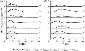
Frequency response to periodic forcing at
 $f_{a}$
with respect to individual hot-wire probes at
 $x=200~\text{mm}$
, for the (a)
 $Re_{{\it\theta}}=850$
(LS) and (b)
 $Re_{{\it\theta}}=1400$
(HS) flow configurations. Duty cycle used is
 $50\,\%$
. Measurements are taken from the spectra of the flow actuated by open-loop in the range of
 $1~\text{Hz}<f_{a}<100~\text{Hz}$
. The horizontal axis denotes the range of actuation frequencies employed. The vertical axis represents the normalized amplitude of power spectral density at the frequency
 $f_{a}$
. Here
 $\text{PSD}(s_{i};f_{a})[f]$
denotes the amplitude of the power spectral density of sensor signal
 $s_{i}$
measured at the frequency of actuation
 $f_{a}$
and
 $P(s_{i};f_{a})$
represents the power of the signal. Values of the vertical axis are shifted by
 $m$
for clarity (where
 $m=0,1,2,3,4,5,6$
). The symbols (see legend) mark the frequencies and the sensors which are selected by the different closed-loop control laws.

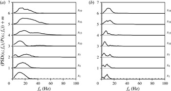
Figure 9 shows amplitudes of power spectral density of the mixing layer flow as a function of the frequency of open-loop actuation
 $\text{PSD}(s_{i};f_{a})$
, for the LS and HS configurations. The amplitude is normalized by the power of the signal. This serves as an estimation of the amplitude of the fluctuations appearing at the frequency of actuation, with respect to the combined amplitudes of fluctuations on all other resolved frequencies.
In figure 9(b), the hot-wires
 $s_{1}$
,
 $s_{4}$
and
 $s_{7}$
are used by the control law
 $\mathscr{F}_{W(HS)}^{GP}$
(3.3). From figure 7 we can see that probe
 $s_{7}$
is dominant in building the actuation signal. In figure 9(b) we note that the most amplified signal that this probe can register, corresponds to the actuation frequency of
 $35~\text{Hz}$
(see legend); exactly what the closed-loop control law selects as the dominant feedback frequency. Moreover, in figure 9(a), we observe that the PSD of the sensor
 $s_{7}$
is maximized for an actuation frequency approximately equal to
 $21~\text{Hz}$
, precisely the frequency found by using the GP control law
 $\mathscr{F}_{W(HS)}^{GP}$
(trained in the HS configuration) in the off-design LS configuration (figure 6
b). This observation suggests that the robust behaviour presented in § 3.3 may result from the dominant role of
 $s_{7}$
, and from the perturbation amplification properties of the actuated mixing layer that makes
 $s_{7}$
sensitive to
 $35~\text{Hz}$
in HS and
 $21~\text{Hz}$
in LS configurations, respectively. Hot-wire probes
 $s_{10}$
to
 $s_{19}$
were not used in the optimal HS control law, but are shown here to illustrate what kind of actuation frequencies they detect. For example, if the control law could be based on
 $s_{10}$
, one might expect a feedback on a frequency from 10 to
 $30~\text{Hz}$
, since these actuation frequencies appear most amplified at this probe’s location (figure 9).
The symbols in figure 9 denote the selected feedback frequencies and the dominant sensors for the closed-loop control laws presented in figures 5, 6 and 8. We can conclude that the frequency selected by using the dominant sensor in the control law is always well amplified. The control law
 $\mathscr{F}_{K(LS)}^{GP}$
(3.2), for example, has sensor
 $s_{19}$
as the dominant sensor and this control always selects a frequency around
 $12~\text{Hz}$
. In figure 9(a), we see that the signature of the open-loop actuation at
 $12~\text{Hz}$
is the most amplified for the sensor
 $s_{19}$
(filled circle). We can make similar statements for the rest of the closed-loop control laws marked on the diagram. In some cases the selected frequency was the most amplified for the sensor in question, but in other cases it was not a maximum. An example is the control law
 $\mathscr{F}_{191(HS)}^{GP}$
(empty circle) in figure 9(b). The frequency selected by this feedback is amplified, but it is not the maximum amplification for this sensor. We can therefore conclude that not only the most amplified, but also sufficiently amplified perturbations can be periodically returned by the feedback control.
The amplification envelopes shown in figure 9 resemble the universal amplification curve, proposed by Fiedler & Mensing (Reference Fiedler and Mensing1985), which follows a nonlinear growth until saturation, then a linear decay. In the case of sensor
 $s_{10}$
, the decay is interrupted by a sudden extinction of amplitude much earlier than for other sensors. This occurs for both LS and HS configurations, albeit for different frequency ranges. As we will discuss in the following § 5.2, this is a consequence of the mean flow modifications induced by the forcing.
We can conclude that the feedback control created by the search process of GP can potentially be based on any frequency
 $f_{a}$
, if the growth rate of the created perturbation estimated for the lock-on condition (
 $f=f_{a}$
) is strictly positive and significant up to and including the location of the feedback sensors.
5.2 Vortex interactions
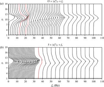
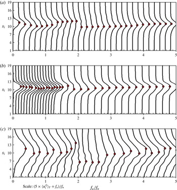
Mean velocity variance profiles (at
 $x=200~\text{mm}$
) in (a)
 $Re_{{\it\theta}}=850$
(LS) and (b)
 $Re_{{\it\theta}}=1400$
(HS) mixing layer configurations, for different open-loop actuation frequencies (
 $0~\text{Hz}<f_{a}<100~\text{Hz}$
,
 $dc=50\,\%$
). Fluctuation magnitudes are scaled and shifted by the value of actuation frequency for clarity. Black dots denote the maximum value of
 $\langle {u_{i}^{\prime }}^{2}(t)\rangle _{T}$
. Variance profiles at open-loop frequencies 12 and 20 Hz, for the LS case, and 35 Hz in the HS case are highlighted in red (colour online only), as being the closest to the best closed-loop solutions presented in § 3.

In this section, we analyse the influence of the actuation frequency
 $f_{a}$
on the structure organization of the forced mixing layer and more precisely on the vortex interactions between the vortices created by the actuator system and those issued from the natural mixing layer. We first turn our attention to the evolution of the velocity variance profiles with respect to a range of open-loop actuation frequencies. The velocity variance profiles for actuation frequencies from 0 to
 $100~\text{Hz}$
are shown in figure 10, for the LS (a) and the HS (b) flow configurations. In both flow configurations, the respective natural profiles feature a single maximum, located between sensors
 $s_{10}$
and
 $s_{13}$
. As the actuation is applied with a progressively higher frequency, the vertical position of the maximum of variance is shifted vertically downwards. The single maximum of fluctuations achieves the lowest vertical position for relatively low frequencies of actuation: 8–10 Hz for LS and around 15 Hz for HS. The downward shift of the maximum of fluctuations indicates that the entrainment of the mixing layer is increased and the mixing layer is vectored towards the low-speed side. If the actuation frequency is still increased past this range, we observe a return of the maximum upwards, and a first appearance of a second, smaller velocity variance maximum. This second maximum starts to be visible from 10 to 12 Hz for the LS case in figure 10(a), and fully emerges as an equal to the first maximum for actuation at approximately 20 Hz. This significant discontinuity in the shape of the profiles appears around the actuation frequencies which maximize objective function
 $W$
. For both flow configurations, this change in the profile shape also corresponds to the abrupt extinction of the normalised PSD amplitude for the sensor
 $s_{10}$
, clearly visible in figure 9(a,b). The variance profiles featuring two maxima of velocity variance can be interpreted as representing the vortex pairing in the mixing layer (Winant & Browand Reference Winant and Browand1974; Ho & Huang Reference Ho and Huang1982). The sensor
 $s_{10}$
is the closest to the middle of the mixing layer and can find itself between two vortices if vortex pairing occurs (one vortex on top of the other, with the hot-wire vertically in between). For the HS case (figure 10
b) this discontinuity is much less pronounced, but is still quite discernible.
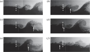
Receding location (indicated by the arrow) of vortex pairing for various open-loop frequencies (from unactuated to 65 Hz) in the HS flow configuration. The approximate streamwise location of the sensor rake is indicated with white crosses. Flow snapshots correspond to: unactuated (a),
 $f_{a}=15$
Hz (b), 5 Hz (c), 30 Hz (d), 10 Hz (e), 65 Hz (f).

It follows that by actuating in a given frequency range, we can promote vortex pairing to occur at the sensor location, while for other actuation frequencies no pairing is observed by the sensors. Smoke visualizations of the flow for several actuation frequencies are shown in figure 11. The selected snapshots all show a typical location of vortex pairing and the associated actuation frequency. We can clearly observe that this location is changing with the actuation frequency and for a certain case it simply coincides with the sensor location. The objective function
 $W$
is designed to select a thick velocity variance profile, and so the optimal control laws aim to cause the vortex pairing which dominates the sensors.
The observed phenomena are in general accordance with the criterion of Moore & Saffman (Reference Moore and Saffman1975) which guarantees a stable vortex arrangement in a turbulent mixing layer. The criterion is
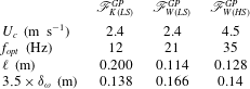
 $\ell \gtrsim 3.5\times {\it\delta}_{{\it\omega}}$
, where
 $\ell$
is the spacing between two vortices, for a single vortex to be stable. In the case of actuated mixing layer, the distance between two vortices is approximated as
 $\ell =U_{c}/f_{opt}$
, where
 $f_{opt}$
is the dominant frequency in the flow resulting from optimal open-loop actuation and the best GP closed-loop control laws. Resulting values are given for reference in table 1 for closed-loop control laws
 $\mathscr{F}_{W(LS)}^{GP}$
(3.1),
 $\mathscr{F}_{K(LS)}^{GP}$
(3.2) and
 $\mathscr{F}_{W(HS)}^{GP}$
(3.3). In the case of maximization of
 $K$
for the LS configuration, the control law produced coherent vortices at a frequency of approximately 12 Hz. In the velocity variance profile (
 $b_{K(LS)}$
in figure 5
a) no sign of vortex pairing is evident, i.e. a single maximum is observed. The corresponding values of
 $\ell$
and
 ${\it\delta}_{{\it\omega}}$
in table 1 show that the criterion for a stable single vortex has been achieved. In contrast, the values of vortex spacing for control laws which maximize
 $W$
are just below the local vorticity thickness criterion. Such values confirm that the vortices have begun to deteriorate due to interaction with the neighbouring vortices, as one would expect when vortex pairing commences. Therefore, the two objective functions are maximized when the controller is triggered either by a large coherent vortex (in the case of
 $K$
) or by a pair of vortices close together (in the case of
 $W$
).
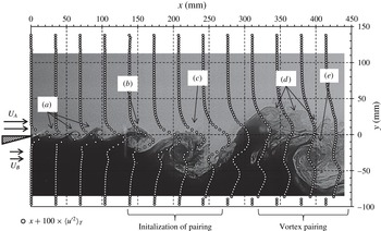
Example of the streamwise evolution of the LS mixing layer actuated with
 $f_{a}=10~\text{Hz}$
. The profiles of averaged streamwise velocity fluctuations
 $\langle {u^{\prime }}^{2}\rangle _{T}$
obtained by particle image velocimetry (PIV) are superimposed over an instantaneous snapshot of smoke visualization of the flow. The profiles which exhibit two peaks correspond to streamwise location where vortex pairing is clearly evident. Upstream of this location, the resurgence of the natural instability (a) can be observed between two cycles of actuation. Vortex (b) is another K–H vortex, already starting to be influenced by the vortex created by actuation (c). The vortex pairing observed at the right-hand side of the frame appears to involve a large vortex (e), created by the previous actuation cycle, as well as several older K–H vortices (d) coalescing around it. The PIV results were obtained using a commercial Dantec system, with a spatial resolution of 3.45 mm between vectors.

Comparison of vortex spacing
 $\ell$
and vorticity thickness
 ${\it\delta}_{{\it\omega}}$
values for the best GP control laws in LS and HS mixing layer configurations. These values are used for estimation of the criterion of stability of a vortex in a turbulent mixing layer
 $\ell \gtrsim 3.5\times {\it\delta}_{{\it\omega}}$
, as given by Moore & Saffman (Reference Moore and Saffman1975).

In addition to vortex pairing, the actuated state can also feature very complex interactions of actuation and natural Kelvin–Helmholtz vortices, as illustrated in figure 12. The visualization shown here, along with the statistically converged data from PIV acquisitions, allow us to shift the analysis from a fixed framework of the hot-wire sensors and explore the spatial development of an actuated mixing layer, albeit for only one frequency of actuation. This example is a typical case of what can be expected to occur when the LS mixing layer is actuated at a low frequency (
 $f_{a}=10~\text{Hz}$
). The wavelength of actuation is so large that it allows a resurgence of the natural instability between two cycles of actuation. In figure 12, several K–H vortices (a) are observed appearing in the wake of the last known actuation vortex (c). Vortex (b) directly in the trail of the actuation vortex (c) is another K–H vortex already starting to be destabilized by the influence of the bigger, turbulent actuation vortex. Further downstream, we can observe older K–H vortices (d) being entrained by a large vortex (e) which is a product of the previous cycle of actuation. The corresponding profiles of
 $\langle u^{\prime 2}\rangle _{T}$
show a typical shape associated with vortex pairing: two peaks of comparable amplitudes. In this case, the pairing occurs around
 $350~\text{mm}<x<450~\text{mm}$
in the streamwise direction. However, the process visible in this example corresponds to the ‘collective interaction’ (Ho & Nosseir Reference Ho and Nosseir1981), where the K–H vortices are entrained around a much larger vortex created by a large amplitude actuation.
5.3 The impact of convection speed on the frequency selection
Since the perturbations produced by actuation dominate the flow, one might expect that the frequency of their repetition by feedback would be locked to a frequency based on the convective time. This does appear to be true for the closed-loop control which maximizes objective function
 $K$
. For the LS configuration, the frequency based on the convective time would be
 $f_{c(LS)}\approx 12~\text{Hz}$
, with respect to
 $U_{c}$
given in the table of figure 1. In § 3.2, the frequency of the closed-loop control law
 $\mathscr{F}_{K(LS)}^{GP}$
is found equal to
 $12~\text{Hz}$
, in agreement with the convective frequency. In the HS case, the corresponding frequency would be
 $f_{c(HS)}\approx 24~\text{Hz}$
. Although the GP was not applied to maximize
 $K$
in the HS configuration, the open-loop mapping in figure 4(d) confirms a maximum of
 $J_{K}$
at
 $(f_{a},dc)_{K(HS)}=(24~\text{Hz},70\,\%)$
, which corresponds to the aforementioned frequency.
However, the speed at which the velocity fluctuations of different length scales are convected is not uniform across the vertical extent of a turbulent mixing layer. Studies by Wills (Reference Wills1964) and most recently by Buxton, de Kat & Ganapathisubramani (Reference Buxton, de Kat and Ganapathisubramani2013) show that a ‘global’ convection velocity, containing all the length scales present in the flow, is similar to the mean velocity profile
 $U(y)$
of the mixing layer, and that fluctuations on the low-speed side convect on average at speeds greater than the mean and fluctuations on the high-speed side are observed to convect at speeds less than the mean. If the local convection characteristics are the only parameters which determine the frequency of feedback, then the vertical location of the sensor might be directly linked with the frequency that the closed-loop control based on that sensor will select.
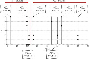
Participation of hot-wire sensors in various control laws and the resulting lock-on frequencies. The filled circles correspond to the sensors appearing in all the individuals matching a particular lock-on frequency. Sensors depicted with empty circles are not dominant, but appear in the control law from which the PSD of the actuation signal has been presented (see figure 8), or whose expression is given in the article (see § 3). The vertical dashed line differentiates between results obtained by tests in the LS configuration, from the results obtained in the HS configuration. Note that the control law
 $\mathscr{F}_{W(HS)}^{GP}$
appears two times, since it was tested in both LS and HS configurations yielding a different selected frequency (see figure 6).

In order to check this hypothesis, we can plot a summary of all of the closed-loop control laws in figure 13. Here we plot the participating sensors in each control law presented so far, versus the lock-on frequency they produce (see § 4). The sensors appearing in all of the matching individuals are referred to as the ‘dominant’ sensors (filled circles). The other sensors which appear in the reference control law are called the ‘supporting’ sensors (empty circles), and they do not appear in all the individuals which match the feedback frequency of the reference control law.
We can immediately recall that the control laws
 $\mathscr{F}_{W(HS)}^{GP}$
and
 $\mathscr{F}_{191(HS)}^{GP}$
share the same dominant sensor
 $s_{7}$
(see § 4.2), but produce different lock-on states (35 and 45 Hz). This already shows that the vertical location of that sensor does not impose a unique feedback frequency, based on the local convection speed.
Furthermore, there appears not to be a link between selecting a sensor on the high-speed side of the mixing layer and obtaining a high-frequency feedback. An obvious example is the control law
 $\mathscr{F}_{238(HS)}^{GP}$
which achieves a lock-on frequency of 32 Hz using only the high-speed side sensor
 $s_{16}$
, whereas
 $\mathscr{F}_{W(HS)}^{GP}$
achieves 35 Hz using always the low-speed side sensor
 $s_{7}$
.
We can conclude that some lock-on states produced by closed-loop control may be related to the convection speed, but certainly not all of them. In addition, the outermost sensors (
 $s_{1}$
and
 $s_{19}$
) are effectively in the far field of the mixing layer for both LS and HS configurations. In their case, the local convection speed observations from Buxton et al. (Reference Buxton, de Kat and Ganapathisubramani2013) probably do not apply. From these results, there is no clear and direct link to be made between the vertical location of the sensors and the selected frequency of feedback. If the feedback control was directly proportional to only one sensor, perhaps the vertical location would be the only parameter. This type of configuration is worth examining in future studies.
In the reported experiment, the transitional stage from the unactuated flow to the fully established actuated lock-on state is not elucidated. It is, however, this transitory period which must be studied in order to fully understand the selected lock-on frequency. It is also worth noting that the selection of the lock-on frequency is very robust. Every time the closed-loop control is activated using the same control law, the resulting lock-on frequency is the same, provided that there is no sensor drift between attempts. In other words, the lock-on state is independent of the unsteady conditions of the flow at the moment the control is activated.
6 Summary and conclusions
The objective of this experimental study was to examine what kind of control laws are physically eligible when closed-loop control of a feedback type is applied in a turbulent mixing layer. In the search for the optimal closed-loop control, the solution space was enlarged by using a model-free GP search/optimization method. GP allows us to search for the possible optimal solutions, without a priori knowledge of what these solutions look like. A critical step is to design an objective function with a unique maximum, which is representative of a distinctive flow state. The GP process will attempt to maximize the imposed objective function by creating and testing many different control laws, to find the most promising candidate.
In our experiments, the actuators are placed at the mixing layer origin, while the sensors are far downstream, in a dominantly convective flow. This arrangement does not allow in-time actuation of the flow dynamics at the sensor location. The instantaneous sensor signals measure the passage of flow structures, which are already far downstream and thus out of reach of the actuator system. However, the closed-loop control can still use the temporal dynamics captured by the sensors to modify the mean flow properties. At the same time, the convective nature of the mixing layer instability requires continual actuation; if the actuation ceases, the mixing layer relaxes into its natural state. Consequently, the mixing layer is continually actuated and the dynamics, captured by the sensors, can be significantly influenced by the signature of the actuation. This leads to a self-repeating feedback cycle, which the closed-loop control laws use to produce a quasiperiodic actuation. The control laws mimic the features of the best open-loop control, without using a fixed time constant. Moreover, the closed loop manages to select the optimal feedback frequency with a high degree of reliability; every time a specific control law is applied to the flow, it produces a synchronized state of the mixing layer with statistically identical properties. This remains true provided the sensor signals do not drift in time, and the flow conditions in the wind tunnel do not change between two tests of the control law.
For each of the two objective functions considered, GP has found distinctly different optimal flow states. When the fluctuation energy
 $K$
is maximized, the optimal flow state features periodic shedding of large coherent vortices at the sensor location. These structures induce an increase of the fluctuation energy across the entire sensor rake, which maximizes the objective function. If the width
 $W$
of the mixing layer has to be maximized, vortex pairing is generated at the sensor location. Thereby, the velocity variance is distributed over a wider range of sensors to satisfy the objective function. The open-loop experiments show that vortex pairing induced by forcing can be observed at different streamwise locations in the mixing layer, depending on the forcing frequency. It is quite remarkable that the closed loop is able to select a feedback frequency which induces the vortex pairing process precisely at the location of the sensors.
At the design point, the objective function values of the optimal periodic forcing and the best GP control laws are identical to within a few per cent. However, under off-design conditions, when the stream velocities are intentionally doubled, the closed-loop control is much more effective compared with the fixed open-loop forcing. The closed loop remains robust by selecting a new feedback frequency to satisfy the objective function. The GP process in our experiments does not use robustness to free-stream velocity changes as a criterion. Nevertheless, the nature of the GP selection process favours control laws which perform well over a large number of tests. This robustness with respect to stochastic fluctuations of the mixing layer flow might also play a role in the observed robustness of the feedback frequency selection when the global conditions change.
By examining the flow under periodic forcing in § 5, we have understood which synchronized states are possible to obtain thanks to the amplification mechanisms of the mixing layer instability. In the case of open-loop control, these states are established by external periodic forcing of our choice. In the case of the closed loop, such states need to be established by the feedback cycle. The closed-loop control permits a limited selection of different feedback frequencies, in spite of being ‘slaved’ to a single streamwise location. In the case of closed-loop control, the desired frequency must be amplified by the mixing layer, otherwise no synchronization is possible. The more the perturbation is amplified, the easier it will be for the feedback controller to produce a periodic signal for actuation. However, the most amplified frequency is not the only one eligible for feedback; other frequencies which are sufficiently amplified can be selected as well. Analyses in the appendix A indicate that the range of obtainable feedback frequencies is inversely proportional to the streamwise location of the sensors.
In order to understand how the closed-loop control synchronizes the mixing layer at different frequencies, the GP control laws functions were analysed with respect to their zero-crossings. Most of the control laws were based around one dominant sensor. However, some control laws were based on the same sensor, yet provoked different feedback frequencies. It therefore follows that the selection of the sensor may have a crucial role, but is not the only factor in the determination of the feedback frequency. The apparently non-essential sensors also contribute by modifying the dominant duty cycle. In this study, there is no observable pattern to the selection of these ‘supporting’ sensors (see § 4.1). Even if we take for granted that the same dominant sensor can provoke a different feedback frequency due to the different scaling imposed by the control law, there is still no clear connection between the vertical location of the selected sensor and the feedback frequency. As we discuss in § 5.3, the different convective speeds of coherent structures, across the vertical domain of the turbulent mixing layer, do not seem to be correlated with the sensor selection.
Finally, a crucial missing link is the process of transition from the unactuated flow to the established feedback state. It is likely that the transition is strongly related with the dynamic response of the mixing layer and the coupling of such response with the location of both the dominant and the supporting sensors. We can only hypothesize that the supporting sensors are used to trigger the initial and several subsequent actuations, leading the perturbations to the dominant sensor, which can then establish the desired feedback cycle. One way to clarify this process would be to model the instantaneous response of the mixing layer to single actuation pulses with specific duty cycles. Our attempts to build such a model, by applying a linear system identification method (ERA/OKID) to the sensor data, have not been successful. From the experimental side a more detailed investigation of the transition phase would need both temporally and spatially resolved flow data, which are out of reach in this study (for example, by time-resolved PIV measurements).
As illustrated by our experiments, the importance of flow control goes beyond obtaining a desired flow state; it also becomes an interesting tool in furthering our knowledge of the flow physics. Model-free control design frameworks such as genetic programming control can prove particularly helpful in this role, since by definition they do not require an a priori knowledge of the flow mechanisms to operate. Such methods can be applied to an unknown plant to extract an optimized control law, which can be analysed to reveal the governing physical mechanisms.
For the improvement of genetic programming and its use for feedback flow control, further efforts should be devoted to introduce methods that automatically balance accuracy and parsimony in the control law. Indeed, the use of arbitrary length representations in GP slows down the evolutionary search process, consumes memory, and even more important for flow control, complicates the understanding of the selection process. In the example of our experiment, some control laws use multiple sensors, and a large number of GP-created individuals are necessary to discover which sensors are crucial to achieve the desired performance. This is much like pinpointing the single gene in a gene sequence, responsible for a specific genetic trait, like the colour of the eyes. Only when a genetic aberration is found for one or few individuals, is it possible to establish the general rule which governs the bulk of the population. A manual selection of the models is generally not feasible. An alternative option is to direct the evolution toward simple models with sufficient accuracy by multiobjective optimization. A recent example is a special version of GP, called Pareto-front GP (Smits & Kotanchek Reference Smits and Kotanchek2005), which has significantly improved the efficiency of symbolic regression model development. The multiobjective optimization framework is, therefore, an appealing approach to determine sparse and robust control laws.
Acknowledgements
We would like to dedicate this work to our late colleagues Carine Fourment and Joël Delville who lost their lives in a road accident, while returning from a research assignment.
This work has been supported by the ANR TUCOROM (ANR-10-CHEX-0015), ANR SepaCoDe (ANR-11-BS09-018) and the ONERA INTACOO grants. M. Segond would like to acknowledge the support of the LINC project (no. 289447) funded by EC’s Marie-Curie ITN program (FP7-PEOPLE-2011-ITN). We appreciate valuable stimulating discussions with the TUCOROM team (D. Barros, J. Borée, E. Kaiser, N. Kutz, R. Li, R. Niven, M. Schlegel and G. Tissot), with the SepaCoDe team, in particular A. Kourta and M. Stanislas, our PMMH collaborators J.-L. Aider and N. Gautier, and O. Cadot, R. King, C. Nayeri, O. Paschereit, R. Radespiel, P. Scholz and R. Semaan. We also thank the referees for many important suggestions.
Appendix A. Impact of the streamwise sensor position
The results presented in the main text are all obtained for a single sensor location at
 $x=200~\text{mm}$
. In this appendix, we show how does the sensor location affect the possibility of establishing a periodic feedback control. In addition, we discuss what would happen if the feedback sensors were at a different streamwise location with respect to the performance evaluation sensors.
Experiments of open-loop mapping and GP-based closed-loop control are performed at
 $x=500~\text{mm}$
, only for the LS mixing layer configuration. The methodology and the general flow conditions are identical as in the main text, except that the vertical position of the sensor rake now covers
 $-104~\text{mm}<y<40~\text{mm}$
with respect to the coordinate system origin at the trailing edge.
Mapping of objective functions
 $J_{W}$
and
 $J_{K}$
for open-loop mapping at
 $x=200~\text{mm}$
(a,c) and
 $x=500~\text{mm}$
(b,d), and four different duty cycles (15 %, 30 %, 50 %, 70 %), in the LS mixing layer configuration.

The receptivity of the mixing layer at this location is tested with open-loop mapping in figure 14, compared to the results obtained previously at
 $x=200~\text{mm}$
. The resulting objective function values follow the expected trends and the maxima are obtained for a lower actuation frequency:
 $(f_{a},dc)_{W(LS,500)}=(9~\text{Hz},50\,\%)$
and
 $(f_{a},dc)_{K(LS,500)}=(5~\text{Hz},70\,\%)$
. The exception is an appearance of a second peak of
 $J_{K}$
for
 $f_{a}\approx 30~\text{Hz}$
. For both objective functions, the authority of actuation is lower at this streamwise location, compared with the results presented in the main text for
 $x=200~\text{mm}$
.
Resulting
 $\langle {u_{i}^{\prime }}^{2}\rangle _{T}$
profiles (a) and pseudovisualizations (b) for maximization of
 $J_{W}$
and
 $J_{K}$
experiments in LS configuration of the mixing layer at
 $x=500~\text{mm}$
. The best open- and closed-loop control are compared. Actuator system input is marked using black and white stripes above each case (black stands for active). The pseudovisualizations are constructed from
 $u_{i}^{\prime }$
in a range of
 $-1.5$
to
 $1.5~(\text{m}~\text{s}^{-1})$
and are based on Taylor’s hypothesis of frozen turbulence.

Figure 15 shows velocity fluctuation profiles and the pseudovisualizations of the natural LS flow, followed by open- and closed-loop control cases for the two objective functions. From visual inspection, the closed-loop control laws
 $\mathscr{F}_{W(LS,500)}^{GP}$
and
 $\mathscr{F}_{K(LS,500)}^{GP}$
appear less periodic than their counterparts from
 $x=200~\text{mm}$
(figure 5). However, the selected dominant frequencies are very close to the open-loop results. In the case of
 $J_{W}$
this is around
 $9~\text{Hz}$
and around
 $4.5~\text{Hz}$
for
 $J_{K}$
. In both cases, the duty cycles are not very well optimized. In the
 $J_{W}$
experiment the closed loop uses a very small duty cycle, while the control law in the
 $J_{K}$
experiment has a larger duty cycle than expected. We can conclude that sensors placement further downstream poses a harder problem to solve for the GP. This is not so surprising since the flow at this streamwise distance is much more unsteady with higher broadband noise levels. This increases the difficulty of obtaining a smooth feedback signal without dedicated filtering. Filtering can be implemented as a feature in GP, but was not available to us at this stage. Regardless of these optimization problems, we can still observe that the closed-loop control managed to perform a good selection of the desired frequencies, even in very adverse conditions.
Frequency response to periodic forcing at
 $f_{a}$
with respect to individual hot-wire probes at (a)
 $x=200~\text{mm}$
and (b)
 $x=500~\text{mm}$
for the LS flow configuration. See figure 9 for the notation.

Mean velocity variance profiles for open-loop actuation frequencies in (a)
 $Re_{{\it\theta}}=850$
(LS) at
 $x=200~\text{mm}$
, (b)
 $Re_{{\it\theta}}=1400$
(HS) at
 $x=200~\text{mm}$
and (c)
 $Re_{{\it\theta}}=850$
(LS) at
 $x=500~\text{mm}$
. The values on the horizontal axis are normalized by the local natural frequency
 $f_{n}$
estimated from
 $St_{{\it\theta}}\approx 0.032$
based on the measured local momentum thickness
 ${\it\theta}$
for each case.

Figure 16 shows a comparison of the frequency response to periodic forcing at the sensor locations (a)
 $x=200~\text{mm}$
and (b)
 $x=500~\text{mm}$
. In the latter case this range is severely truncated, and we can expect that a feedback control could select only frequencies lower than
 $15~\text{Hz}$
. Therefore, we can surmise that the second maximum of
 $J_{K}$
observable in figure 14 at approximately
 $30~\text{Hz}$
would not be obtainable by the closed-loop control.
In figure 17 we show mean velocity variance profiles for different open-loop actuation frequencies for three experiments. This figure is similar to figure 10 except for the addition of the LS experiment performed at
 $x=500~\text{mm}$
and the normalization of the values on the horizontal axis. Now, the horizontal axis is normalized by an estimated local frequency
 $f_{n}$
based on the measured
 ${\it\theta}$
at the sensor location. We can observe that in all three cases the vortex pairing at the location of the sensors is achieved when the actuation frequency is approaching twice the value of the estimated local natural frequency, i.e.
 $f_{a}/f_{n}\approx 2$
. If, on the other hand, the actuation is near the local natural frequency
 $f_{a}/f_{n}\approx 1$
, we obtain a maximum of fluctuation energy
 $K$
. However, since we cannot really observe a single, well-defined, natural frequency (see § 3.1), we caution the reader that this scaling is presented only as a guideline to the general similarity of the mean flow modifications for the cases shown.
The combined results (for the LS flow configuration) for the two studied locations of the sensor array allow us to discuss how would the closed-loop control work if the feedback sensors and the performance evaluation sensors were placed at different streamwise locations. For example, if the effects on the objective function would be estimated at
 $x=500~\text{mm}$
, the control targets would be 5 and
 $9~\text{Hz}$
for the
 $J_{K}$
and
 $J_{W}$
, respectively (after the data in figure 14). According to the frequency response to periodic forcing at
 $x=200~\text{mm}$
(figure 16
a), these low frequencies should be obtainable by the closed-loop control. At this upstream location,
 $5~\text{Hz}$
seems to be amplified well for the sensor
 $s_{7}$
, while
 $9~\text{Hz}$
should be obtainable through several sensors, especially those farther from the middle of the mixing layer. Therefore, a closed-loop control receiving information from an upstream sensor could be constructed to maximize an objective function at a given downstream location.
Can this work in the opposite case, i.e. can we pick up information on the feedback sensor which is placed far downstream and optimize an objective function for an upstream location? Objective function
 $J_{W}$
is maximized by a
 $21~\text{Hz}$
actuation at
 $x=200~\text{mm}$
(figure 14
a), which does not appear as an amplified frequency to any of the hot-wire sensors at
 $x=500~\text{mm}$
in figure 16(b). In other words, such a frequency cannot be filtered from the sensors at this streamwise length and a feedback cycle will not be established. On the other hand, the optimal actuation frequency of
 $12~\text{Hz}$
for the maximization of
 $J_{K}$
at
 $x=200~\text{mm}$
is still very visible by the sensors at
 $x=500~\text{mm}$
. In this case, we could expect a working closed-loop control to be established.
To conclude, a closed-loop feedback control based on two arrays of sensors at different streamwise locations can obtain a lock-on state only for the actuation frequencies which are amplified on both locations. The target frequency must be amplified at the location of the feedback sensors in order to establish a periodic feedback. At the same time, it must also be amplified at the location of the performance evaluation sensors, otherwise it would not be able to modify the flow toward a desired lock-on state.
Appendix B. Genetic programming in the experiment
This appendix provides more information about the GPC framework. We also discuss specific aspects of implementation of GP in the mixing layer experiment.
GP is a biologically inspired algorithm where the genetic operators (replication, mutation and cross-over) operate on a set of operations, elementary functions, variables and constants. When GP is used for symbolic regression, it combines automatically these elements to search for a symbolic expression that constitutes the best solution to a given optimization problem. Proposed symbolic expressions (examples shown in figure 18) are built as tree-like structures (Koza Reference Koza1992) which can be easily evaluated in a recursive manner and described by a Lisp expression. These trees are called individuals, while a population of individuals is a generation. GP is implemented as an iterative procedure in which a population of candidate solutions evolves toward better solutions by repeatedly undergoing genetic modifications based on their fitness.
The first generation of individuals is created in a random manner. All individuals are evaluated and a fitness value is attributed based on how well they minimize or maximize the objective function. A second generation of individuals is then created using three principal genetic operations: replication, mutation and cross-over. Each of the genetic operations occurs with a predetermined probability. If replication is selected as an operation to be performed, the candidate individual will simply be copied into the next generation (figure 18 a). Mutation causes a part of the individual’s tree to be replaced by a newly created random subtree as shown in figure 18(b). A cross-over operation involves a pair of individuals, which will exchange a randomly selected subtree between each other and two new individuals created in such a manner will become a part of the next generation (figure 18 c).
Biologically inspired operations performed by GP on the tree-like functions: (a) replication, (b) mutation and (c) cross-over. The tree represented in (a) corresponds to the function
 $b(t)=\text{C}\times s_{1}(t)+\exp (s_{2}(t))$
where
 $\text{C}$
is a constant to be determined by GP. For the mutation (b), the operation consists of selecting a node, erasing its subtree and replacing it by another one created randomly. Part of the information contained in the individual is kept while new information is allowed to enter the population. Mutation increases the diversity and is responsible for exploring the search space with large steps. For the cross-over (c), one node in each of the two individuals selected for the cross-over is randomly chosen, the nodes and their subtrees are then exchanged. The cross-over is responsible for exploring the search space around well-performing individuals.

The selection process of candidate individuals uses the tournament method; few random individuals are chosen to compete in a tournament and the winner (based on its evaluated fitness) is selected for one of the genetic operations to be performed on it. The tournament is an efficient way of controlling the selectiveness of the GP evolutionary process. Usually, the size of the tournament is small compared with the size of the population. The bigger the tournament size
 $N_{t}$
is, the more probable it is to include the overall best individuals as participants, leading to a more selective process. The selection ranges from a random individual for
 $N_{t}=1$
, to selection of the best individual of the generation if
 $N_{t}$
equals the size of the population of the current generation.
An additional operation available is elitism, which copies the single or few best individuals of one generation directly into the next generation, while avoiding the tournament process. This operation is generally used to ensure that the best individuals of one generation are not lost and remain available for further improvements in the future generations.
When all the individuals of the next generation are created, they are evaluated and the selection process begins anew in order to build a subsequent generation. This iterative process continues for a desired number of generations. A rule of thumb is that given a sufficient number of individuals in each generation, a solution should be obtained in less than
 $N_{g}=50$
generations. There is no mathematical proof of convergence, but the method has been successful in many applications (Lewis, Fagg & Solidum Reference Lewis, Fagg and Solidum1992; Nordin & Banzhaf Reference Nordin and Banzhaf1997).
The genetic programming part of GPC code is developed in-house based on an open-source code ECJ (Luke et al. Reference Luke, Panait, Balan, Paus, Skolicki, Kicinger, Popovici, Sullivan, Harrison and Bassett1993). Genetic programming codes using numerical simulations as evaluation data do not need to evaluate the same individual more than once. In the experiment, however, one is faced with uncertainties and stochasticity created by natural perturbations in the flow and the actuator system, measurement precision, etc. In order to be better adapted to experimental conditions, our GPC code contains crucial new features.
-
(1) An individual is evaluated every time it appears in the genetic programming process.
-
(2) The cost of an individual is averaged with the values recorded previously for the same individual, resulting in a cumulative moving average being used as the cost function value.
-
(3) A predetermined number of best individuals in each generation is re-evaluated several more times (five in our case) to ensure a stable sample size for the averaging process.
-
(4) No duplicate individuals are allowed during the creation of the first generation.
The GP learning module thus assigns a cumulative average cost function value (fitness) to an individual. The objective is to choose as the best individual, one which has a continuously good performance, rather than one with strongly varying performance due to external perturbations. Such perturbations may cause an undeserved high fitness value to be attributed to an otherwise unremarkable individual, which is the only real danger to the convergence process. The averaged cost approach is designed to promote robustness and prevent such events from having an influence, but at a price of being much more conservative in the selection of individuals. As a consequence, the control laws which are attributed with high values of fitness are those which also perform consistently well, which also means that the control laws themselves are selected to be more robust to stochastic perturbations.
Operations and elementary functions used in the experiment are:
 $+$
,
 $-$
,
 $\times$
,
 $/$
,
 $\sin$
,
 $\cos$
,
 $\exp$
,
 $\tanh$
and
 $\log$
. Sensitive operations such as
 $/$
and
 $\log$
are protected so that any value in
 $\mathbb{R}$
can be used as arguments. The variables available to GP are instantaneous values of velocity fluctuations from the hot-wire sensors i.e.
 $s_{i}(t)\equiv u_{i}^{\prime }(t)$
. Every third sensor in the rake is used as a variable since more would only carry redundant information for the sensor-based controller. Hence,
 $n_{s}=19$
for the evaluation of the cost functions (2.1a,b
), while only
 $7$
sensors across the shear layer are employed in the construction of the control laws
 $\mathscr{F}^{GP}$
. Finally, constants used are in a range of
 $[-1,1]$
with a precision up to a second decimal. The range and precision are adapted to be of the same order of magnitude as the typical velocity fluctuation information given by the sensors.
In the experiment, the standard rates for the genetic programming operations are 0 % for replication, 65 % for mutation and 35 % for cross-over. Elitism is set to
 $N_{e}=5$
, meaning that five best individuals in a generation are sent directly to the next generation. An experiment consists of
 $N_{g}=25$
generations, where each generation is composed of
 $N_{i}=50$
individuals. An individual is limited to a minimum tree depth of
 $2$
and a maximum tree depth of
 $10$
levels.
At the start of each generation, the unactuated flow and the best open-loop actuation are retested in order to keep track of these reference values. Hence, each individual’s cost (
 $J_{K}$
or
 $J_{W}$
) is calculated using the reference baseline flow values (
 $K_{u}$
or
 $W_{u}$
) obtained at the beginning of its own generation.
The evaluation time of every individual in the experiment is
 $T=10~\text{s}$
, while there is up to 6 s of various delays in order to facilitate communication between the learning module, the controller and the data recording system. Also, a few seconds must be allowed for the mixing layer to register the effects of each new actuation when changing individuals during the learning process. Taking this into account, a single evaluation of an individual takes around 20 s to complete. A standard GPC experiment of 25 generations is completed in approximately 10 h. However, depending on the parameters of the genetic operations, the optimal solution in our experiments emerges even after four to six generations. This is equivalent to approximately 2.5 h of wind tunnel time. With some experience and knowledge of the controlled plant, quick optimization tests can be performed without too much time investment.