1 Introduction
The prospects of creating magnetically confined electron–positron (pair) plasmas in dipole or stellarator geometries have been discussed since early 2000s (Pedersen et al.
Reference Pedersen, Boozer, Dorland, Kremer and Schmitt2003, Reference Pedersen, Danielson, Hugenschmidt, Marx, Sarasola, Schauer, Schweikhard, Surko and Winkler2012). In the near future, the first experiment APEX (A Positron-Electron EXperiment) will be constructed to confine such plasmas in a magnetic dipole geometry (Saitoh et al.
Reference Saitoh, Stanja, Stenson, Hergenhahn, Niemann, Pedersen, Stoneking, Piochacz and Hugenschmidt2015). Recently, efficient injection and trapping of a cold positron beam in a dipole magnetic field configuration has been demonstrated by Saitoh et al. (Reference Saitoh, Stanja, Stenson, Hergenhahn, Niemann, Pedersen, Stoneking, Piochacz and Hugenschmidt2015) using a supported permanent magnet. This result is a key step towards the ultimate aim of creating and studying the first man-made magnetically confined pair plasma in the laboratory. To achieve this, a device is now planned consisting of a cylindrical ca. 20 l vacuum vessel and a levitated coil. The electrons are to be injected with an electron gun and the positrons will be supplied from an already existing neutron source at the Technical University of Munich. One expects the following plasma parameters: plasma densities in the range
 $10^{10}~\text{m}^{-3}<n<10^{12}~\text{m}^{-3}$
, temperatures in the range
 $1~\text{eV}<T<10~\text{eV}$
, a Debye length
 $\unicode[STIX]{x1D706}_{D}=\sqrt{\unicode[STIX]{x1D716}_{0}T/(2ne^{2})}<10^{-2}~\text{m}$
and a gyroradius satisfying
 $\unicode[STIX]{x1D70C}\ll \unicode[STIX]{x1D706}_{D}$
. The plasmas will have very small pressure, i.e.
 $\unicode[STIX]{x1D6FD}=\unicode[STIX]{x1D707}_{0}nT/B^{2}\ll 1$
.
It has been shown by Helander (Reference Helander2014) that pair plasmas possess unique stability properties due to the mass symmetry between the particle species. For example, drift instabilities are completely absent in straight-field-line geometry, e.g. in a slab, provided that the temperature and density profiles of the two species are equal (‘symmetric’ pair plasmas). The symmetry between the species is broken if the temperature profiles of the electrons and positrons differ or there is an ion contamination. Then, the drift instabilities can be excited (Mishchenko et al. Reference Mishchenko, Zocco, Helander and Könies2018) even in an unsheared slab geometry. In a sheared slab, pure pair plasmas are prone to current-driven reconnecting instabilities, see (Chacón et al. Reference Chacón, Simakov, Lukin and Zocco2008; Zocco Reference Zocco2017) and references therein. It is clear that also in this case there is an asymmetry between the species since the ambient electron flow velocity must differ from the positron one for the ambient current to be finite. In contrast to a slab geometry, a dipole magnetic field has finite curvature. In this case, the symmetry between the species is broken by the curvature drifts and the plasma can be driven unstable for certain values of the temperature and density gradients (Helander Reference Helander2014), even without ion contamination and for identical temperature profiles of the two species. This result persists also in the electromagnetic regime (Helander & Connor Reference Helander and Connor2016). The nonlinear stability of dipole pair plasmas has also been addressed recently by Helander (Reference Helander2017).
Over the years, there have been a number of magnetic dipole experiments using conventional proton–electron plasmas, such as the Levitated Dipole Experiment (LDX) at MIT (Kesner et al. Reference Kesner, Bromberg, Garnier and Mauel1999), the Collisionless Terrella Experiment (CTX) at Columbia University (Warren & Mauel Reference Warren and Mauel1995), the Large Magnetic Mirror Experiment (LAMEX) at UCLA (Ferron et al. Reference Ferron, Wong, Dimonte and Leikind1983) and the Ring Trap-1 (RT-1) experiment at the University of Tokyo (Yoshida et al. Reference Yoshida, Saitoh, Morikawa, Yano, Watanabe and Ogawa2010). A large amount of work in the areas of plasma equilibrium, stability and transport has been done for such plasmas, which can serve as a useful reference for the study of pair plasmas in a magnetic dipole geometry (Krasheninnikov, Catto & Hazeltine Reference Krasheninnikov, Catto and Hazeltine1999; Krasheninnikov & Catto Reference Krasheninnikov and Catto2000; Simakov et al. Reference Simakov, Catto, Krasheninnikov and Ramos2000a ; Simakov, Hastie & Catto Reference Simakov, Hastie and Catto2000b ; Kesner et al. Reference Kesner, Simakov, Garnier, Catto, Hastie, Krasheninnikov, Mauel, Pedersen and Ramos2001; Simakov, Catto & Hastie Reference Simakov, Catto and Hastie2001; Wong et al. Reference Wong, Horton, Van Dam and Crabtree2001; Kesner & Hastie Reference Kesner and Hastie2002; Simakov et al. Reference Simakov, Catto, Ramos and Hastie2002a ; Simakov, Hastie & Catto Reference Simakov, Hastie and Catto2002b ; Krasheninnikova & Catto Reference Krasheninnikova and Catto2006; Ricci, Rogers & Dorland Reference Ricci, Rogers and Dorland2006a ; Ricci et al. Reference Ricci, Rogers, Dorland and Barnes2006b ; Kouznetsov, Freidberg & Kesner Reference Kouznetsov, Freidberg and Kesner2007; Kobayashi, Rogers & Dorland Reference Kobayashi, Rogers and Dorland2009, Reference Kobayashi, Rogers and Dorland2010; Porazik & Lin Reference Porazik and Lin2011; Xie et al. Reference Xie, Zhang, Huang, Ou and Li2017).
In this paper, we focus on pair plasmas, extending the results of Helander (Reference Helander2014) by performing a detailed study of the drift-kinetic stability of a pure pair plasma in a dipole geometry, making use of both the Z-pinch and point-dipole limits, where the dispersion relation is derived, analysed and numerically solved. We find that the parameter space of the instability can be characterised by two asymptotes: the resonant stability boundary, corresponding to the vanishing growth rate, and the fluid stability boundary. The latter reduces to a ‘singularity boundary’ with infinite growth rates when the finite-Debye-length effects are neglected. This finding can be compared with previous results concerning the resonant stability boundary corresponding to the entropy mode (Simakov et al. Reference Simakov, Catto and Hastie2001; Ricci et al. Reference Ricci, Rogers, Dorland and Barnes2006b ) and the fluid stability boundary corresponding to the electrostatic interchange mode (Kesner et al. Reference Kesner, Simakov, Garnier, Catto, Hastie, Krasheninnikov, Mauel, Pedersen and Ramos2001; Simakov et al. Reference Simakov, Catto and Hastie2001). The structure of the paper is as follows. In § 2, we introduce the magnetic dipole field and discuss the near-magnetic-axis (Z-pinch) and far-field (point-dipole) limits. In § 3, we introduce the linear drift-kinetic description and derive a ‘master’ equation, applicable to both Z-pinch and point-dipole limits. The Z-pinch and point-dipole limits are then individually treated in §§ 4 and 5, respectively. The conclusions are summarised in § 6.
2 Dipole magnetic field
In cylindrical coordinates
 $(r,\unicode[STIX]{x1D711},z)$
, the magnetic field of a circular conducting loop with the radius
 $r_{0}$
carrying the total current
 $I$
is
 $$\begin{eqnarray}\displaystyle \boldsymbol{B}(r,z)=\unicode[STIX]{x1D735}\unicode[STIX]{x1D713}(r,z)\times \unicode[STIX]{x1D735}\unicode[STIX]{x1D711},\quad \unicode[STIX]{x1D735}\unicode[STIX]{x1D711}=\frac{\boldsymbol{e}_{\unicode[STIX]{x1D711}}}{r}, & & \displaystyle\end{eqnarray}$$
with the poloidal magnetic flux given by (Landau & Lifshitz Reference Landau and Lifshitz1960; Simpson et al. Reference Simpson, Lane, Immer and Youngquist2001)
 $$\begin{eqnarray}\unicode[STIX]{x1D713}(r,z)=\frac{C}{2}\,\sqrt{(r_{0}+r)^{2}+z^{2}}\left[\frac{r_{0}^{2}+r^{2}+z^{2}}{(r_{0}+r)^{2}+z^{2}}K(\unicode[STIX]{x1D705})-E(\unicode[STIX]{x1D705})\right],\quad C=\frac{\unicode[STIX]{x1D707}_{0}I}{\unicode[STIX]{x03C0}},\end{eqnarray}$$
where
 $\unicode[STIX]{x1D707}_{0}$
is the magnetic permeability of free space. The elliptic integrals of the first and the second kind,
 $$\begin{eqnarray}K(\unicode[STIX]{x1D705})=\int _{0}^{1}\frac{\text{d}x}{\sqrt{(1-x^{2})(1-\unicode[STIX]{x1D705}^{2}x^{2})}},\quad E(\unicode[STIX]{x1D705})=\int _{0}^{1}\frac{\sqrt{1-\unicode[STIX]{x1D705}^{2}x^{2}}}{\sqrt{1-x^{2}}}\,\text{d}x,\end{eqnarray}$$
depend on the parameter
 $\unicode[STIX]{x1D705}$
defined in (2.4). Following Simpson et al. (Reference Simpson, Lane, Immer and Youngquist2001)
 $$\begin{eqnarray}\unicode[STIX]{x1D705}^{2}=1-\unicode[STIX]{x1D70C}^{2}/\unicode[STIX]{x1D6FD}^{2},\quad \unicode[STIX]{x1D70C}^{2}=(r-r_{0})^{2}+z^{2},\quad \unicode[STIX]{x1D6FD}^{2}=(r_{0}+r)^{2}+z^{2}.\end{eqnarray}$$
The components of the magnetic field are then expressed
 $$\begin{eqnarray}\displaystyle B_{r} & = & \displaystyle \frac{Cz}{2\unicode[STIX]{x1D70C}^{2}\unicode[STIX]{x1D6FD}r}\left[(r_{0}^{2}+r^{2}+z^{2})E(\unicode[STIX]{x1D705}^{2})-\unicode[STIX]{x1D70C}^{2}K(\unicode[STIX]{x1D705}^{2})\right]\end{eqnarray}$$
 $$\begin{eqnarray}\displaystyle B_{z} & = & \displaystyle \frac{C}{2\unicode[STIX]{x1D70C}^{2}\unicode[STIX]{x1D6FD}}\left[(r_{0}^{2}-r^{2}-z^{2})E(\unicode[STIX]{x1D705}^{2})+\unicode[STIX]{x1D70C}^{2}K(\unicode[STIX]{x1D705}^{2})\right].\end{eqnarray}$$
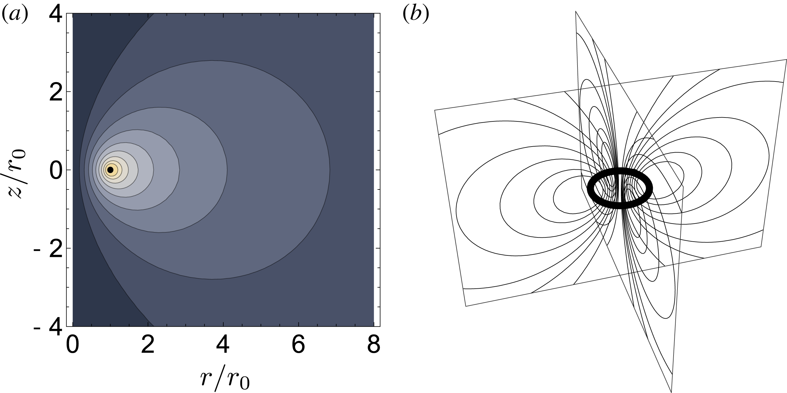
(a) is a plot of
 $\unicode[STIX]{x1D713}(r,z)$
, as defined in (2.2). Magnetic field lines (here, represented by contours of constant
 $\unicode[STIX]{x1D713}$
) are generated by the circular coil at
 $(r,z)=(r_{0},0)$
, whose cross-section is shown here as a small black disk. In the yellow region, close to the coil, the field is approximately that of a Z pinch, whereas in the grey region, far from the coil, it approaches the field of a point dipole. (b) is a three-dimensional cartoon of a dipole magnetic field.

We will consider two asymptotic cases of this magnetic geometry, depicted in figure 1. The first case arises in the region close to the current loop. This is the Z-pinch limit, corresponding to
 $$\begin{eqnarray}\frac{r-r_{0}}{r_{0}}\sim \frac{z}{r_{0}}\sim \frac{\unicode[STIX]{x1D70C}}{r_{0}}\ll 1.\end{eqnarray}$$
In this case,
 $\unicode[STIX]{x1D6FD}\approx 2r_{0}$
so that
 $\unicode[STIX]{x1D705}\rightarrow 1$
(Gradshteyn & Ryzhik Reference Gradshteyn and Ryzhik1980) and
 $$\begin{eqnarray}E(\unicode[STIX]{x1D705})\approx 1,\quad K(\unicode[STIX]{x1D705})\approx \ln \left(\frac{4}{\sqrt{1-\unicode[STIX]{x1D705}^{2}}}\right)\approx -\ln \left(\frac{\unicode[STIX]{x1D70C}}{8r_{0}}\right).\end{eqnarray}$$
Substituting these relations into (2.5) and (2.6), we obtain
 $$\begin{eqnarray}B_{r}\approx \frac{Cz}{2\unicode[STIX]{x1D70C}^{2}},\quad B_{z}\approx -\frac{C(r-r_{0})}{2\unicode[STIX]{x1D70C}^{2}},\quad \unicode[STIX]{x1D713}=-\frac{Cr_{0}}{2}\ln \left(\frac{\unicode[STIX]{x1D70C}}{8r_{0}}\right).\end{eqnarray}$$
Here, we employed
 $\unicode[STIX]{x1D70C}\ll r_{0}$
and invoked
 $$\begin{eqnarray}\lim _{x\rightarrow 0}x\ln x=0\Rightarrow \frac{\unicode[STIX]{x1D70C}}{r_{0}}\ln \left(\frac{\unicode[STIX]{x1D70C}}{r_{0}}\right)\ll 1.\end{eqnarray}$$
Introducing a new ‘quasi-polar’ coordinate system, with the axis corresponding to the magnetic axis (the current loop), we define the new ‘quasi-polar’ angle
 $\unicode[STIX]{x1D701}$
satisfying
 $$\begin{eqnarray}\sin \unicode[STIX]{x1D701}=\frac{z}{\unicode[STIX]{x1D70C}},\quad \cos \unicode[STIX]{x1D701}=\frac{r-r_{0}}{\unicode[STIX]{x1D70C}},\quad \boldsymbol{e}_{\unicode[STIX]{x1D701}}=\frac{\unicode[STIX]{x1D735}\unicode[STIX]{x1D701}}{|\unicode[STIX]{x1D735}\unicode[STIX]{x1D701}|}=-\boldsymbol{e}_{r}\sin \unicode[STIX]{x1D701}+\boldsymbol{e}_{z}\cos \unicode[STIX]{x1D701}.\end{eqnarray}$$
In these notations, the magnetic field becomes
 $$\begin{eqnarray}B_{r}=\frac{\unicode[STIX]{x1D707}_{0}I}{2\unicode[STIX]{x03C0}\unicode[STIX]{x1D70C}}\sin \unicode[STIX]{x1D701},\quad B_{z}=-\frac{\unicode[STIX]{x1D707}_{0}I}{2\unicode[STIX]{x03C0}\unicode[STIX]{x1D70C}}\cos \unicode[STIX]{x1D701},\quad \boldsymbol{B}=-\frac{\unicode[STIX]{x1D707}_{0}I}{2\unicode[STIX]{x03C0}\unicode[STIX]{x1D70C}}\boldsymbol{e}_{\unicode[STIX]{x1D701}}.\end{eqnarray}$$
This is the usual Z-pinch magnetic field, created by a linear current flowing in the axial direction.
The second case to be considered corresponds to the far-field limit. For this case, the spherical coordinate system
 $(\hat{r},\hat{\unicode[STIX]{x1D703}},\unicode[STIX]{x1D711})$
, with
 $\hat{r}$
the spherical radial distance,
 $\hat{\unicode[STIX]{x1D703}}$
the azimuthal angle and
 $\unicode[STIX]{x1D711}$
the polar angle, is more convenient. For
 $\hat{r}\gg r_{0}$
, the magnetic field is
 $$\begin{eqnarray}B_{r}\approx \frac{2M\cos \hat{\unicode[STIX]{x1D703}}}{\hat{r}^{3}},\quad B_{\unicode[STIX]{x1D703}}\approx \frac{M\sin \hat{\unicode[STIX]{x1D703}}}{\hat{r}^{3}},\quad \unicode[STIX]{x1D713}=\frac{M\sin ^{2}\hat{\unicode[STIX]{x1D703}}}{\hat{r}},\quad M=\frac{\unicode[STIX]{x1D707}_{0}Ir_{0}^{2}}{4}.\end{eqnarray}$$
These expressions are called the ‘point-dipole approximation’, valid far from the current loop. We neglect the pressure effects (Krasheninnikov et al.
Reference Krasheninnikov, Catto and Hazeltine1999; Krasheninnikov & Catto Reference Krasheninnikov and Catto2000) on the ambient magnetic field throughout the paper. This can be done since
 $\unicode[STIX]{x1D6FD}\ll 1$
is expected in the pair plasma experiment under construction (Saitoh et al.
Reference Saitoh, Stanja, Stenson, Hergenhahn, Niemann, Pedersen, Stoneking, Piochacz and Hugenschmidt2015).
3 Drift-kinetic theory
Following Helander (Reference Helander2014) and Helander & Connor (Reference Helander and Connor2016), we begin with gyrokinetic theory. It is convenient to write the gyrokinetic distribution function in the form:
 $$\begin{eqnarray}f_{a}=f_{a0}\left(1-\frac{e_{a}\unicode[STIX]{x1D719}}{T_{a}}\right)+g_{a}=f_{a0}+f_{a1},\quad f_{a1}=-\frac{e_{a}\unicode[STIX]{x1D719}}{T_{a}}\,f_{a0}+g_{a}.\end{eqnarray}$$
Here,
 $f_{a0}$
is a Maxwellian,
 $a$
is the species index with
 $a=e$
corresponding to the electrons,
 $a=p$
to the positrons. The linearised gyrokinetic equation in this notation is
 $$\begin{eqnarray}\text{i}v_{\Vert }\unicode[STIX]{x1D735}_{\Vert }g_{a}+(\unicode[STIX]{x1D714}-\unicode[STIX]{x1D714}_{\text{d}a})g_{a}=\frac{e_{a}}{T_{a}}\,\text{J}_{0}\left(\frac{k_{\bot }v_{\bot }}{\unicode[STIX]{x1D714}_{\text{c}a}}\right)\,(\unicode[STIX]{x1D714}-\unicode[STIX]{x1D714}_{\ast a}^{\text{T}})\,\unicode[STIX]{x1D719}\,f_{a0},\end{eqnarray}$$
with
 $\text{J}_{0}$
the Bessel function,
 $\unicode[STIX]{x1D714}_{\text{c}a}$
the cyclotron frequency,
 $k_{\bot }$
the perpendicular wavenumber and
 $\unicode[STIX]{x1D719}$
the perturbed electrostatic potential. The notation used is summarised as follows:
 $$\begin{eqnarray}\displaystyle & \displaystyle \unicode[STIX]{x1D714}_{\ast a}^{\text{T}}=\unicode[STIX]{x1D714}_{\ast a}\left[1+\unicode[STIX]{x1D702}_{a}\left(\frac{v^{2}}{v_{\text{th}a}^{2}}-\frac{3}{2}\right)\right],\quad v=\sqrt{v_{\Vert }^{2}+v_{\bot }^{2}},\quad \unicode[STIX]{x1D707}=\frac{m_{a}v_{\bot }^{2}}{2B} & \displaystyle\end{eqnarray}$$
 $$\begin{eqnarray}\displaystyle & \displaystyle \unicode[STIX]{x1D714}_{\ast a}=\frac{k_{\unicode[STIX]{x1D711}}T_{a}}{e_{a}}\frac{\text{d}\ln n_{a}}{\text{d}\unicode[STIX]{x1D713}},\quad \unicode[STIX]{x1D702}_{a}=\frac{\text{d}\ln T_{a}}{\text{d}\ln n_{a}},\quad v_{\text{th}a}=\sqrt{\frac{2T_{a}}{m_{a}}},\quad \unicode[STIX]{x1D714}_{\text{c}a}=\frac{e_{a}B}{m_{a}} & \displaystyle\end{eqnarray}$$
 $$\begin{eqnarray}\displaystyle & \displaystyle \unicode[STIX]{x1D714}_{\text{d}a}=\boldsymbol{k}_{\bot }\boldsymbol{\cdot }\boldsymbol{v}_{\text{d}a},\quad \boldsymbol{v}_{\text{d}a}=(mv_{\Vert }^{2}+\unicode[STIX]{x1D707}B)\,\frac{\boldsymbol{b}\times \unicode[STIX]{x1D735}B}{e_{a}B^{2}},\quad \boldsymbol{k}_{\bot }=k_{\unicode[STIX]{x1D713}}\unicode[STIX]{x1D735}\unicode[STIX]{x1D713}+k_{\unicode[STIX]{x1D711}}\unicode[STIX]{x1D735}\unicode[STIX]{x1D711}. & \displaystyle\end{eqnarray}$$
Here,
 $\unicode[STIX]{x1D713}$
is the poloidal flux and
 $\unicode[STIX]{x1D711}$
is the polar (toroidal) angle. We choose the sign convention such that
 $\unicode[STIX]{x1D714}_{\ast e}\geqslant 0$
for the electrons and
 $\unicode[STIX]{x1D714}_{\ast p}\leqslant 0$
for the positrons. We will assume the drift-kinetic limit in what follows, i.e.
 $k_{\bot }v_{\text{th}a}/\unicode[STIX]{x1D714}_{\text{c}a}\ll 1$
so
 $\text{J}_{0}\approx 1$
.
We expand the distribution function
 $g_{a}=g_{a}^{(0)}+g_{a}^{(1)}+\cdots \,$
in the small parameter
 $\unicode[STIX]{x1D700}_{b}=\unicode[STIX]{x1D714}/\unicode[STIX]{x1D714}_{b}$
where
 $\unicode[STIX]{x1D714}_{b}$
is the bounce frequency. To lowest order, we obtain
 $$\begin{eqnarray}v_{\Vert }\unicode[STIX]{x1D735}_{\Vert }g_{a}^{(0)}=0\end{eqnarray}$$
implying that
 $g_{a}^{(0)}$
coincides with its bounce average,
 $g_{a}^{(0)}=\overline{g}_{a}^{(0)}$
, where the bounce-average operation is defined as
 $$\begin{eqnarray}\left.\overline{(\ldots )}=\oint (\ldots )\frac{\text{d}l}{v_{\Vert }}\right/\oint \frac{\text{d}l}{v_{\Vert }}.\end{eqnarray}$$
Here,
 $l$
is the arc length measured along a magnetic field line and the integration is performed between bounce points for trapped particles, and over the entire closed field line for passing particles. Note that there are only trapped particles in the point-dipole limit and only passing particles in the Z-pinch limit. Applying the bounce average at the next order in
 $\unicode[STIX]{x1D700}_{b}$
, we obtain
 $$\begin{eqnarray}(\unicode[STIX]{x1D714}-\overline{\unicode[STIX]{x1D714}}_{\text{d}a})g_{a}^{(0)}=(\unicode[STIX]{x1D714}-\unicode[STIX]{x1D714}_{\ast a}^{\text{T}})\frac{e_{a}\overline{\unicode[STIX]{x1D719}}}{T_{a}}f_{a0}.\end{eqnarray}$$
We assume the temperature and the density profiles of the electrons and the positrons to be identical, and invoke the Poisson equation for the charge density perturbations, given by the distribution functions
 $f_{a1}$
:
 $$\begin{eqnarray}\left(\mathop{\sum }_{a=e,p}\frac{n_{a}e_{a}^{2}}{T_{a}}+\unicode[STIX]{x1D716}_{0}\,k_{\bot }^{2}\right)\unicode[STIX]{x1D719}=\mathop{\sum }_{a=e,p}e_{a}\int g_{a}^{(0)}\,\text{d}^{3}v.\end{eqnarray}$$
Note that
 $g_{a}\ll f_{a0}$
so that all terms in (3.9) can be of the same order. We find that the perturbed electrostatic potential satisfies the equation:
 $$\begin{eqnarray}(1+k_{\bot }^{2}\unicode[STIX]{x1D706}_{D}^{2})\unicode[STIX]{x1D719}=\frac{1}{n_{0}}\int \frac{\unicode[STIX]{x1D714}^{2}-\overline{\unicode[STIX]{x1D714}}_{d}\unicode[STIX]{x1D714}_{\ast }^{\text{T}}}{\unicode[STIX]{x1D714}^{2}-\overline{\unicode[STIX]{x1D714}}_{d}^{2}}\overline{\unicode[STIX]{x1D719}}\,f_{0}\,\text{d}^{3}v.\end{eqnarray}$$
Here and in the following, we use the notation
 $\unicode[STIX]{x1D714}_{\ast }^{\text{T}}\equiv \unicode[STIX]{x1D714}_{\ast e}^{\text{T}}$
,
 $\unicode[STIX]{x1D714}_{\ast }\equiv \unicode[STIX]{x1D714}_{\ast e}$
,
 $\overline{\unicode[STIX]{x1D714}}_{d}\equiv \overline{\unicode[STIX]{x1D714}}_{\text{d}e}$
,
 $n_{0}=n_{e}$
,
 $T_{0}\equiv T_{e}$
, and the Debye length is defined as usual,
 $\unicode[STIX]{x1D706}_{D}=\sqrt{\unicode[STIX]{x1D716}_{0}T_{0}/(2n_{0}e^{2})}$
.
For the pair plasmas expected in APEX, the densities will be small implying that the collisions are relatively unimportant (Saitoh et al. Reference Saitoh, Stanja, Stenson, Hergenhahn, Niemann, Pedersen, Stoneking, Piochacz and Hugenschmidt2015). Therefore, we can neglect collisions in this paper. The gyroradius is also expected to be much smaller than the Debye length so that finite Larmor radius (FLR) effects can be considered negligible. In contrast, the Debye length will not be as small as it usually is in fusion experiments, although it will still be much smaller than the system size. This relative importance of the Debye length for the particular case of the pair plasmas expected in the APEX (Saitoh et al. Reference Saitoh, Stanja, Stenson, Hergenhahn, Niemann, Pedersen, Stoneking, Piochacz and Hugenschmidt2015) motivates our interest in this effect.
Summarising, (3.10) is to be considered the ‘master’ equation for drift-kinetic stability in magnetic dipole geometry. It will be solved in Z-pinch and point-dipole limits, to give insight into the general properties of the stability of symmetric pair plasmas in a magnetic dipole geometry. We note also that, in addition to the connection with previous results concerning ion–electron plasmas, as mentioned in the introduction, (3.10) (and all the subsequent results) can be seen to apply exactly for sub-ion-bounce-frequency instabilities in symmetric (equal temperature) electron–ion plasmas, also satisfying
 $k_{\bot }^{-1}\sim \unicode[STIX]{x1D706}_{D}\gg \unicode[STIX]{x1D70C}_{i}$
(the species labels need not even be adjusted since this equation is written in terms of electron quantities).
4 Z-pinch case
In the Z-pinch limit, the components (in polar coordinates) of the magnetic field and the perpendicular wave vector, i.e.
 $\boldsymbol{B}\boldsymbol{\cdot }\boldsymbol{e}_{\unicode[STIX]{x1D701}}$
and
 $\boldsymbol{k}_{\bot }\boldsymbol{\cdot }\boldsymbol{e}_{\unicode[STIX]{x1D701}}$
, etc. are flux functions. In this case, there is no particle trapping, and the orbit average of the perturbed electrostatic potential
 $\bar{\unicode[STIX]{x1D719}}$
coincides with its field-line average
 $\langle \unicode[STIX]{x1D719}\rangle$
 $$\begin{eqnarray}\langle \unicode[STIX]{x1D719}\rangle =\left.\oint \unicode[STIX]{x1D719}\,\text{d}l\right/\oint \text{d}l.\end{eqnarray}$$
Taking the field-line average of (3.10), one can perform the velocity integrals appearing there analytically following Biglari, Diamond & Rosenbluth (Reference Biglari, Diamond and Rosenbluth1989). This results in
 $$\begin{eqnarray}\displaystyle 1+k_{\bot }^{2}\unicode[STIX]{x1D706}_{D}^{2}=\frac{1}{2}(D_{+}+D_{-}),\quad D_{\pm }=\frac{1}{\sqrt{\unicode[STIX]{x03C0}}}\int \frac{\unicode[STIX]{x1D6FA}\mp \unicode[STIX]{x1D6FA}_{\ast }^{\text{T}}}{\unicode[STIX]{x1D6FA}\mp {x_{\bot }}^{2}/2\mp {x_{\Vert }}^{2}}\exp (-x^{2})\,x_{\bot }\,\text{d}x_{\bot }\,\text{d}x_{\Vert }, & & \displaystyle \nonumber\\ \displaystyle & & \displaystyle\end{eqnarray}$$
where we write
 $\unicode[STIX]{x1D714}_{d}=\hat{\unicode[STIX]{x1D714}}_{d}({x_{\Vert }}^{2}+x_{\bot }^{2}/2)$
,
 $\unicode[STIX]{x1D6FA}=\unicode[STIX]{x1D714}/\hat{\unicode[STIX]{x1D714}}_{d}$
,
 $x=\sqrt{{x_{\Vert }}^{2}+{x_{\bot }}^{2}}$
,
 $\unicode[STIX]{x1D6FA}_{\ast }^{\text{T}}=\unicode[STIX]{x1D714}_{\ast }^{\text{T}}/\hat{\unicode[STIX]{x1D714}}_{d}=\unicode[STIX]{x1D6FA}_{\ast }[1+\unicode[STIX]{x1D702}(x^{2}-3/2)]$
, and
 $\unicode[STIX]{x1D6FA}_{\ast }=\unicode[STIX]{x1D714}_{\ast }/\hat{\unicode[STIX]{x1D714}}_{d}$
. Note that the function
 $D_{+}$
was obtained by Biglari et al. (Reference Biglari, Diamond and Rosenbluth1989), and here we generalise their calculation to obtain
 $D_{-}$
, which arises because of the sign difference between the ion (positron here) and the (non-adiabatic) electron drifts. To compute this function, one can perform the same integrals, but with the complex frequency in the lower half-plane. We find
 $$\begin{eqnarray}D_{\pm }(\unicode[STIX]{x1D6FA})=Y_{\pm }^{2}+\unicode[STIX]{x1D6FA}_{\ast }\left\{\left[\pm \frac{\unicode[STIX]{x1D702}-1}{\unicode[STIX]{x1D6FA}}-2\unicode[STIX]{x1D702}\right]Y_{\pm }^{2}\pm 2\unicode[STIX]{x1D702}Y_{\pm }\right\},\end{eqnarray}$$
where
 $$\begin{eqnarray}\displaystyle & \displaystyle Y_{+}(\unicode[STIX]{x1D6FA})=\int _{\infty }^{\unicode[STIX]{x1D6FA}}\frac{\text{d}z}{\sqrt{z}}\exp (z-\unicode[STIX]{x1D6FA})=-\sqrt{\unicode[STIX]{x1D6FA}}Z(\sqrt{\unicode[STIX]{x1D6FA}}), & \displaystyle\end{eqnarray}$$
 $$\begin{eqnarray}\displaystyle & \displaystyle Y_{-}(\unicode[STIX]{x1D6FA})=\int _{-\infty }^{\unicode[STIX]{x1D6FA}}\frac{\text{d}z}{\sqrt{z}}\exp (\unicode[STIX]{x1D6FA}-z)=\sqrt{\unicode[STIX]{x1D6FA}}\left[2\text{i}\sqrt{\unicode[STIX]{x03C0}}\exp (\unicode[STIX]{x1D6FA})-\text{i}Z(-\text{i}\sqrt{\unicode[STIX]{x1D6FA}})\right], & \displaystyle\end{eqnarray}$$
and
 $Z$
is the plasma dispersion function. When
 $\text{Im}[\unicode[STIX]{x1D6FA}]>0$
,
 $\sqrt{\unicode[STIX]{x1D6FA}}$
is defined as the principal root (which lies in the upper half-plane). To treat Landau damping,
 $Y_{\pm }$
must be analytically continued to perform the contour integral in the inversion of the Laplace transform. In particular, we must choose the branch of
 $\sqrt{\unicode[STIX]{x1D6FA}}$
so that the function remains analytic. Very closely related problems were treated by Sugama (Reference Sugama1999) and Helander et al. (Reference Helander, Mishchenko, Kleiber and Xanthopoulos2011), who chose the branch cut of the function
 $\sqrt{\unicode[STIX]{x1D6FA}}$
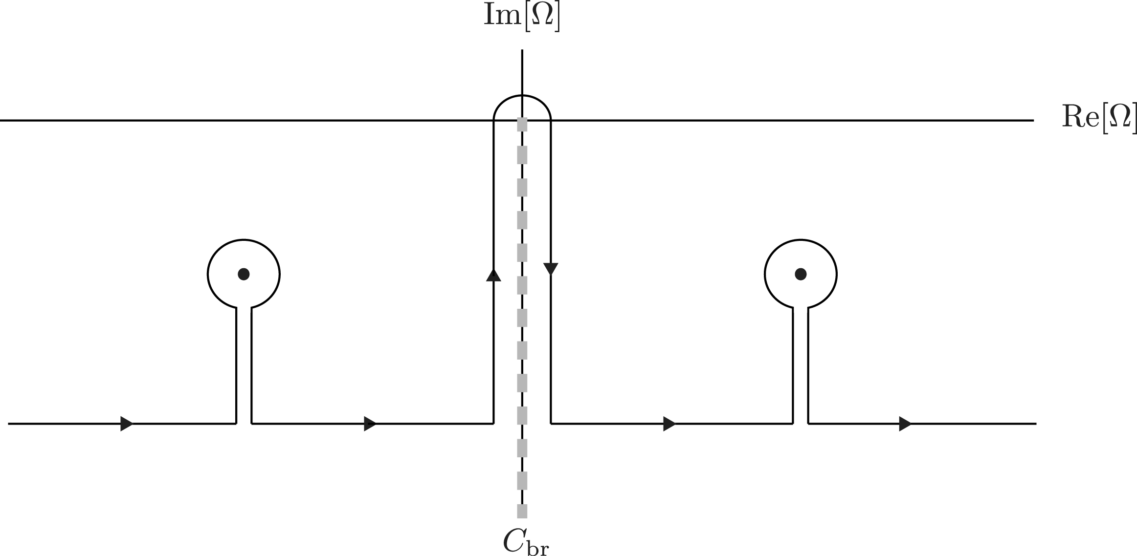
to lie along the negative imaginary axis. This approach allows pole contributions to be picked up in the usual fashion, with an additional contribution coming from integration along the branch cut; see figure 2.
Landau contour appearing in Sugama (Reference Sugama1999) and Helander et al. (Reference Helander, Mishchenko, Kleiber and Xanthopoulos2011). The branch cut is the grey dashed line labelled as
 $C_{\text{br}}$
.

In the present case we take a different approach, namely to perform the integral in the
 $\sqrt{\unicode[STIX]{x1D6FA}}$
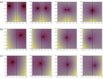
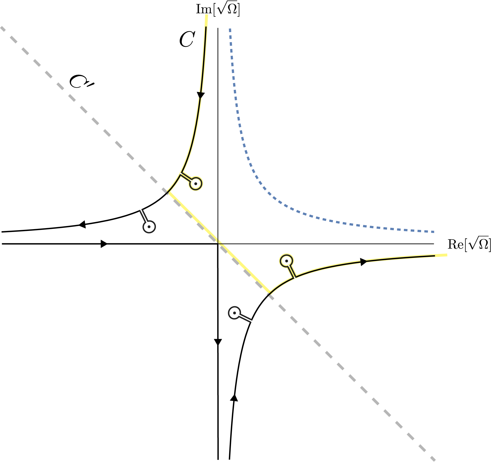
plane, in which it is possible to continue the dispersion function analytically over the entire plane, avoiding the need for a branch cut. The reason for this choice is that the pole contributions can cross the negative imaginary axis, and therefore evade detection; a case where this happens is shown in figure 3. The new contour for Laplace inversion is shown in figure 4. In this figure, the curved paths are contours of constant
 $\text{Im}[\unicode[STIX]{x1D6FA}]$
. Thus, the standard curve for inverting a Laplace transform is shown in dashed blue. The new contour is chosen so that it lies in the upper left and lower right quadrants, where
 $\text{Im}[\unicode[STIX]{x1D6FA}]<0$
. The curved portions of the path can be neglected as compared to the pole contributions, for the usual reason that the corresponding part of the solution is damped more strongly than the pole contributions.
Density plot of dispersion function
 $1+k_{\bot }^{2}\unicode[STIX]{x1D706}_{D}^{2}-(D_{+}+D_{-})/2$
in the complex
 $\unicode[STIX]{x1D6FA}$
plane. Poles are observed to cross the negative imaginary axis as
 $k_{\bot }^{2}\unicode[STIX]{x1D706}_{D}^{2}$
is varied. Here
 $\unicode[STIX]{x1D702}=10$
,
 $\unicode[STIX]{x1D6FA}_{\ast }=1$
, and the values of
 $k_{\bot }^{2}\unicode[STIX]{x1D706}_{D}^{2}$
are
 $6$
,
 $8$
,
 $10$
and
 $12$
. (a) Symmetrised case: branch cut of
 $\sqrt{\unicode[STIX]{x1D6FA}}$
lies on negative imaginary axis. Both poles present until they cross the branch cut and are lost. (b) With branch cut of
 $\sqrt{\unicode[STIX]{x1D6FA}}$
placed on negative real axis, one pole can be found. (c) With branch cut of
 $\sqrt{\unicode[STIX]{x1D6FA}}$
placed on positive real axis, one pole can be found.

As was found by Sugama (Reference Sugama1999) and Helander et al. (Reference Helander, Mishchenko, Kleiber and Xanthopoulos2011), part of the integral causes algebraic damping, while the pole contributions, i.e. the complex mode frequencies, can be obtained as the roots of (4.2). In the present case, the algebraic damping comes from the integral running along the negative
 $\text{Re}[\sqrt{\unicode[STIX]{x1D6FA}}]$
and
 $\text{Im}[\sqrt{\unicode[STIX]{x1D6FA}}]$
axes. The long-time limit of this contribution is dominated by the
 $\unicode[STIX]{x1D6FA}\rightarrow 0$
point, and goes as
 $1/t^{2}$
. We further note that this algebraic contribution corresponds to integrals along the real axis in the
 $\unicode[STIX]{x1D6FA}$
plane. Thus, the damping can be assured to be non-exponential, and any exponential damping comes explicitly from the identified poles.
Extended Landau contour,
 $C$
. Note that the negative imaginary
 $\unicode[STIX]{x1D6FA}$
axis is mapped to the grey dashed line, labelled
 $C^{\prime }$
, and the contour of figure 2 is shown in light yellow for comparison. Note that the path of figure 2 does not encircle the depicted poles that lie beneath
 $C^{\prime }$
, which is why we use the modified contour here.

In practice, the consequence of the above discussion is that the complex frequency of Landau-damped modes is determined by roots of the dispersion function
 $1+k_{\bot }^{2}\unicode[STIX]{x1D706}_{D}^{2}-(D_{+}+D_{-})/2$
that lie in either the upper-left or lower-right quadrant in the complex
 $\sqrt{\unicode[STIX]{x1D6FA}}$
plane. Landau damping will occur at sufficiently large values of
 $k_{\bot }\unicode[STIX]{x1D706}_{D}$
.
At
 $k_{\bot }\unicode[STIX]{x1D706}_{D}\lesssim 1$
, the fluid limit
 $\unicode[STIX]{x1D6FA}\gg 1$
can be applied to (4.2), yielding the solution
 $$\begin{eqnarray}\unicode[STIX]{x1D714}^{2}=-\frac{\hat{\unicode[STIX]{x1D714}}_{d}^{2}}{k_{\bot }^{2}\unicode[STIX]{x1D706}_{D}^{2}}\left[(1+\unicode[STIX]{x1D702})\frac{\unicode[STIX]{x1D714}_{\ast }}{\hat{\unicode[STIX]{x1D714}}_{d}}-\frac{7}{4}\right].\end{eqnarray}$$
One sees that this equation can satisfy the drift-kinetic ordering
 $\unicode[STIX]{x1D714}\ll \unicode[STIX]{x1D714}_{ca}$
implied throughout the paper despite the fact that
 $\unicode[STIX]{x1D6FA}\gg 1$
. Note that
 $\hat{\unicode[STIX]{x1D714}}_{d}$
is proportional to
 $k_{\bot }$
and can be estimated as
 $\hat{\unicode[STIX]{x1D714}}_{d}\sim (k_{\bot }\unicode[STIX]{x1D70C}_{s})\unicode[STIX]{x1D714}_{t}$
where
 $\unicode[STIX]{x1D714}_{t}$
is the transit frequency and
 $\unicode[STIX]{x1D70C}_{s}$
is the thermal gyroradius. This observation, applied to (4.6), gives the following estimate:
 $$\begin{eqnarray}\frac{\unicode[STIX]{x1D714}}{\unicode[STIX]{x1D714}_{t}}\sim \frac{\hat{\unicode[STIX]{x1D714}}_{d}}{k_{\bot }\unicode[STIX]{x1D706}_{D}}\sim \frac{\unicode[STIX]{x1D70C}_{s}}{\unicode[STIX]{x1D706}_{D}}.\end{eqnarray}$$
In the pair plasma of experimental interest
 $\unicode[STIX]{x1D70C}_{s}\ll \unicode[STIX]{x1D706}_{D}$
. In this case,
 $\unicode[STIX]{x1D714}\ll \unicode[STIX]{x1D714}_{c}$
is easily satisfied since
 $\unicode[STIX]{x1D714}_{t}/\unicode[STIX]{x1D714}_{c}\sim \unicode[STIX]{x1D70C}_{s}/r_{0}$
, with
 $r_{0}$
being the radius of the Z pinch, and
 $$\begin{eqnarray}\frac{\unicode[STIX]{x1D714}}{\unicode[STIX]{x1D714}_{c}}\sim \frac{\unicode[STIX]{x1D70C}_{s}^{2}}{r_{0}\unicode[STIX]{x1D706}_{D}}\ll 1.\end{eqnarray}$$
Only for extremely small
 $\unicode[STIX]{x1D706}_{D}\rightarrow 0$
, the inequality (4.8) will be violated. Luckily, such cases are irrelevant for the experiment.
Note that the temperature and density gradients act in (4.6) together (via the factor
 $1+\unicode[STIX]{x1D702}$
), and a purely density-gradient-driven mode is possible, similar to Simakov et al. (Reference Simakov, Catto and Hastie2001). This fluid mode most closely resembles a collisionless electrostatic interchange instability, however with the Debye length assuming the role of the ion Larmor radius (see equation (5) of Ricci et al. (Reference Ricci, Rogers, Dorland and Barnes2006b
)). Equation (4.6) implies the ‘fluid’ instability condition (which is the singularity boundary if
 $k_{\bot }\unicode[STIX]{x1D706}_{D}=0$
exactly):
 $$\begin{eqnarray}\frac{\unicode[STIX]{x1D714}_{\ast }}{\hat{\unicode[STIX]{x1D714}}_{d}}(1+\unicode[STIX]{x1D702})>\frac{7}{4}.\end{eqnarray}$$
Note, however, that the threshold condition
 $\unicode[STIX]{x1D714}=0$
contradicts the ‘fluid’ assumption
 $\unicode[STIX]{x1D6FA}\gg 1$
made above. It indicates that higher-order terms may be needed to treat the plasma stability at the ‘fluid stability boundary’. Even when
 $\unicode[STIX]{x1D714}_{\ast }$
exceeds
 $\hat{\unicode[STIX]{x1D714}}_{d}$
sufficiently for the existence of an unstable ‘fluid’ mode, the mode must succumb to Landau damping for sufficiently large
 $k_{\bot }\unicode[STIX]{x1D706}_{D}$
. We can take
 $\unicode[STIX]{x1D6FA}\sim 1$
to estimate the wavenumber where this transition must occur:
 $$\begin{eqnarray}k_{\bot }\unicode[STIX]{x1D706}_{D}\sim \left|\frac{7}{4}-(1+\unicode[STIX]{x1D702})\frac{\unicode[STIX]{x1D714}_{\ast }}{\hat{\unicode[STIX]{x1D714}}_{d}}\right|^{1/2}.\end{eqnarray}$$
For values of
 $k_{\bot }\unicode[STIX]{x1D706}_{D}$
exceeding this, we return to the Landau damping problem.
We can also derive the ‘resonant stability boundary’ taking
 $\unicode[STIX]{x1D6FA}\rightarrow 0$
in (4.2), obtaining
 $$\begin{eqnarray}\frac{\unicode[STIX]{x1D714}_{\ast }}{\hat{\unicode[STIX]{x1D714}}_{d}}(1-\unicode[STIX]{x1D702})=\frac{1+k_{\bot }^{2}\unicode[STIX]{x1D706}_{D}^{2}}{\unicode[STIX]{x03C0}}.\end{eqnarray}$$
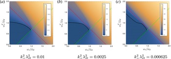
As it turns out, the true stability boundary runs along portions each of the two stability boundaries, equations (4.9) and (4.11), as demonstrated in figure 5.
Stability diagram for several values of
 $k_{\bot }^{2}\unicode[STIX]{x1D706}_{D}^{2}$
, compared with theoretical stability boundaries. The colour of the density plot corresponds to numerically obtained growth rate (dark blue is zero and large positive values are yellow). The region of absolute stability is darkened and bordered by a solid black contour. The theoretical stability lines (dashed red, and dashed green) correspond respectively to (4.9) and (4.11). Note that the deviation from the red theoretical stability boundary (which does not include finite-
 $k_{\bot }\unicode[STIX]{x1D706}_{D}$
corrections) decreases as
 $k_{\bot }^{2}\unicode[STIX]{x1D706}_{D}^{2}\rightarrow 0$
, although surprisingly slowly.

5 Point-dipole case
Now we turn to dipole geometry. In contrast to the Z-pinch limit, the magnetic field strength and perpendicular wave vector change along field lines in the dipole geometry, i.e.
 $B=B(\unicode[STIX]{x1D713},l)$
and
 $k_{\bot }=k_{\bot }(\unicode[STIX]{x1D713},l)$
, etc., depend on
 $\unicode[STIX]{x1D713}$
the poloidal flux and
 $l$
the distance measured along a field line. It has been shown by Kesner & Hastie (Reference Kesner and Hastie2002) that the bounce-averaged drift frequency in the point dipole can be approximated with very good accuracy as
 $\overline{\unicode[STIX]{x1D714}}_{d}\approx 4k_{\unicode[STIX]{x1D711}}mv^{2}/(3e\unicode[STIX]{x1D713})$
. Using this approximation, the integrals in (3.10) can be factorised into velocity (
 $v$
) and pitch-angle (
 $\unicode[STIX]{x1D706}$
) parts:
 $$\begin{eqnarray}(1+k_{\bot }^{2}\unicode[STIX]{x1D706}_{D}^{2})\unicode[STIX]{x1D719}=\unicode[STIX]{x1D6EC}\int _{0}^{1/B}\frac{B\,\text{d}\unicode[STIX]{x1D706}}{\sqrt{1-\unicode[STIX]{x1D706}B}}\bar{\unicode[STIX]{x1D719}},\quad \unicode[STIX]{x1D6EC}=\frac{1}{n_{0}}\int _{0}^{\infty }\frac{\unicode[STIX]{x1D714}^{2}-\overline{\unicode[STIX]{x1D714}}_{d}\unicode[STIX]{x1D714}_{\ast }^{\text{T}}}{\unicode[STIX]{x1D714}^{2}-\overline{\unicode[STIX]{x1D714}}_{d}^{2}}f_{0}2\unicode[STIX]{x03C0}v^{2}\,\text{d}v.\end{eqnarray}$$
In this section, we will focus on the growing solutions with
 $\unicode[STIX]{x1D6FE}=-\text{i}\unicode[STIX]{x1D714}>0$
. To begin, we assume
 $k_{\bot }\unicode[STIX]{x1D706}_{D}\rightarrow 0$
and employ the relations:
 $$\begin{eqnarray}\oint \text{d}l\mathop{\int }_{0}^{1/B}\frac{\text{d}\unicode[STIX]{x1D706}}{\sqrt{1-\unicode[STIX]{x1D706}B}}\overline{\unicode[STIX]{x1D719}}=2\,\oint \frac{\text{d}l}{B}\unicode[STIX]{x1D719},\quad \overline{\unicode[STIX]{x1D719}}(\unicode[STIX]{x1D706})=\frac{1}{\displaystyle \oint \frac{\text{d}l}{\sqrt{1-\unicode[STIX]{x1D706}B}}}\oint \frac{\unicode[STIX]{x1D719}\,\text{d}l}{\sqrt{1-\unicode[STIX]{x1D706}B}}.\end{eqnarray}$$
In this case, the dispersion relation is simply
 $\unicode[STIX]{x1D6EC}=1/2$
. Expressing the velocity integrals through the plasma dispersion function
 $Z_{0}(\unicode[STIX]{x1D701})$
, we obtain
 $$\begin{eqnarray}\displaystyle & \displaystyle \unicode[STIX]{x1D6EC}=\frac{1}{2}\left[\frac{\unicode[STIX]{x1D714}_{\ast }\unicode[STIX]{x1D702}}{\unicode[STIX]{x1D714}\unicode[STIX]{x1D701}}\overline{Z}_{6}(\unicode[STIX]{x1D701})+\frac{\unicode[STIX]{x1D714}_{\ast }}{\unicode[STIX]{x1D714}\unicode[STIX]{x1D701}}\left(1-\frac{3\unicode[STIX]{x1D702}}{2}\right)\overline{Z}_{4}(\unicode[STIX]{x1D701})-\unicode[STIX]{x1D701}\overline{Z}_{2}(\unicode[STIX]{x1D701})\right],\quad \tilde{\unicode[STIX]{x1D714}}_{d}=\frac{4k_{\unicode[STIX]{x1D711}}T}{3e\unicode[STIX]{x1D713}} & \displaystyle\end{eqnarray}$$
 $$\begin{eqnarray}\displaystyle & \displaystyle \unicode[STIX]{x1D701}=\sqrt{\frac{\unicode[STIX]{x1D714}}{2\tilde{\unicode[STIX]{x1D714}}_{d}}},\quad \overline{Z}_{n}(\unicode[STIX]{x1D701})=Z_{n}(\unicode[STIX]{x1D701})+\text{i}Z_{n}(\text{i}\unicode[STIX]{x1D701}),\quad Z_{n}(\unicode[STIX]{x1D701})=\frac{1}{\sqrt{\unicode[STIX]{x03C0}}}\int _{-\infty }^{\infty }\frac{x^{n}e^{-x^{2}}\,\text{d}x}{x-\unicode[STIX]{x1D701}}, & \displaystyle\end{eqnarray}$$
which leads to the dispersion relation
 $$\begin{eqnarray}\frac{\unicode[STIX]{x1D714}_{\ast }\unicode[STIX]{x1D702}}{\unicode[STIX]{x1D714}\unicode[STIX]{x1D701}}\overline{Z}_{6}+\frac{\unicode[STIX]{x1D714}_{\ast }}{\unicode[STIX]{x1D714}\unicode[STIX]{x1D701}}\left(1-\frac{3\unicode[STIX]{x1D702}}{2}\right)\overline{Z}_{4}-\unicode[STIX]{x1D701}\overline{Z}_{2}=1.\end{eqnarray}$$
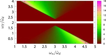
Growth rate
 $\unicode[STIX]{x1D6FE}$
plotted as a function of
 $\unicode[STIX]{x1D714}_{n}$
and
 $\unicode[STIX]{x1D714}_{T}$
. The diamagnetic frequencies
 $\unicode[STIX]{x1D714}_{n}$
and
 $\unicode[STIX]{x1D714}_{T}$
are normalised to the drift frequency
 $\tilde{\unicode[STIX]{x1D714}}_{d}$
. The colours indicate the values of
 $\unicode[STIX]{x1D6FE}$
(see the legend on right). One sees that the growth rate increases strongly towards the ‘singularity boundary’, defined in (5.7).

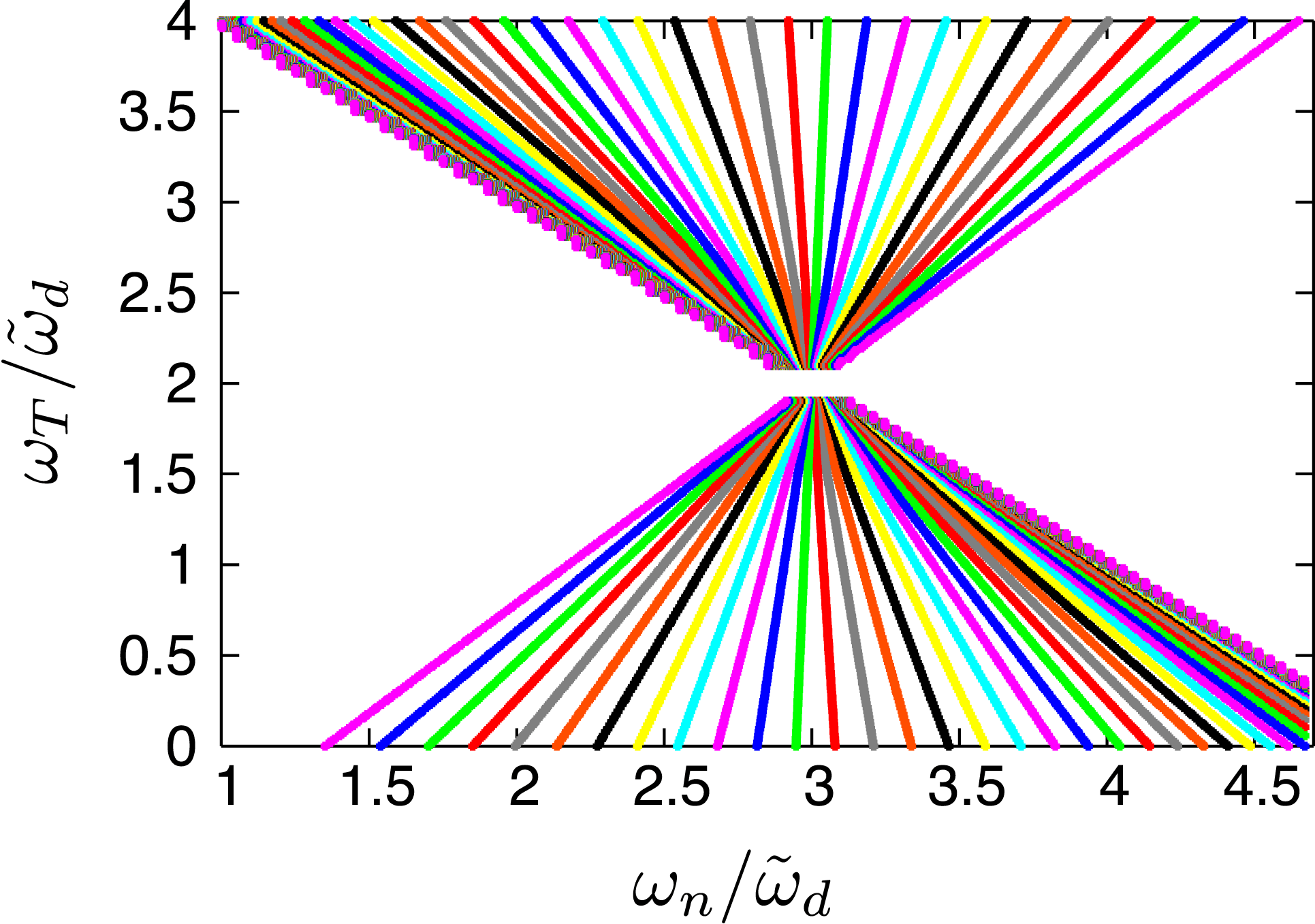
Contours of constant growth rate
 $\unicode[STIX]{x1D6FE}$
plotted in the two-dimensional parameter space
 $(\unicode[STIX]{x1D714}_{n},\unicode[STIX]{x1D714}_{T})$
. The diamagnetic frequencies
 $\unicode[STIX]{x1D714}_{n}$
and
 $\unicode[STIX]{x1D714}_{T}$
are normalised to the drift frequency
 $\tilde{\unicode[STIX]{x1D714}}_{d}$
. Different colours indicate different values of
 $\unicode[STIX]{x1D6FE}$
. The density of the contours shows how fast the growth rate changes. Note that this density is especially high near the ‘singularity boundary’, defined in (5.7).

Taking the limit
 $\unicode[STIX]{x1D701}\rightarrow 0$
, we find the ‘stability’ boundary (Helander Reference Helander2014):
 $$\begin{eqnarray}\frac{\unicode[STIX]{x1D714}_{n}-\unicode[STIX]{x1D714}_{T}}{\tilde{\unicode[STIX]{x1D714}}_{d}}=1,\quad \unicode[STIX]{x1D714}_{n}=\unicode[STIX]{x1D714}_{\ast },\quad \unicode[STIX]{x1D714}_{T}=\unicode[STIX]{x1D702}\unicode[STIX]{x1D714}_{\ast }.\end{eqnarray}$$
Taking the opposite limit
 $\unicode[STIX]{x1D701}\rightarrow \infty$
, we find the ‘singularity’ boundary:
 $$\begin{eqnarray}\frac{\unicode[STIX]{x1D714}_{n}+\unicode[STIX]{x1D714}_{T}}{\tilde{\unicode[STIX]{x1D714}}_{d}}=5\quad \Leftrightarrow \quad \frac{\text{d}\ln (nT)}{\text{d}\ln \unicode[STIX]{x1D713}}=\frac{20}{3}.\end{eqnarray}$$
In agreement with Simakov et al. (Reference Simakov, Catto and Hastie2001), Kesner et al. (Reference Kesner, Simakov, Garnier, Catto, Hastie, Krasheninnikov, Mauel, Pedersen and Ramos2001), the singularity boundary coincides with the magneto-hydrodynamic (MHD) stability threshold (Helander & Connor Reference Helander and Connor2016), although (5.7) has been obtained within the electrostatic formalism. Both the stability and the singularity boundaries can be seen in the numerical solution of the dispersion relation (5.5), shown in figures 6 and 7. Here, the value of the growth rate
 $\unicode[STIX]{x1D6FE}$
(see figure 6) and the contours of constant
 $\unicode[STIX]{x1D6FE}$
(see figure 7) are plotted in the two-dimensional parameter space
 $(\unicode[STIX]{x1D714}_{n},\unicode[STIX]{x1D714}_{T})$
. The colour palette in figure 6 shows how the value of the growth rate changes with
 $\unicode[STIX]{x1D714}_{n}$
and
 $\unicode[STIX]{x1D714}_{T}$
. Different colours in figure 7 just indicate different values of the growth rate. The density of the contours in figure 7 shows how fast the growth rate changes. One sees that this density of the contours is especially high near the singularity boundary. The numerical solutions of (5.5) in the domain bounded by (5.6) and (5.7) represent all unstable modes with finite growth rates.
Similar studies have been previously carried out in proton–electron plasmas confined by a dipole magnetic field (Kesner et al. Reference Kesner, Simakov, Garnier, Catto, Hastie, Krasheninnikov, Mauel, Pedersen and Ramos2001; Simakov et al. Reference Simakov, Catto and Hastie2001). There, the stability diagrams have been plotted in terms of the parameters:
 $$\begin{eqnarray}\unicode[STIX]{x1D702}=\frac{\unicode[STIX]{x1D714}_{T}}{\unicode[STIX]{x1D714}_{n}},\quad d=\frac{\unicode[STIX]{x1D714}_{n}}{3\widetilde{\unicode[STIX]{x1D714}}_{d}}(1+\unicode[STIX]{x1D702}).\end{eqnarray}$$
For comparison, we can express our stability parameters as
 $$\begin{eqnarray}\frac{\unicode[STIX]{x1D714}_{T}}{\widetilde{\unicode[STIX]{x1D714}}_{d}}=\frac{3\unicode[STIX]{x1D702}d}{1+\unicode[STIX]{x1D702}},\quad \frac{\unicode[STIX]{x1D714}_{n}}{\widetilde{\unicode[STIX]{x1D714}}_{d}}=\frac{3d}{1+\unicode[STIX]{x1D702}},\end{eqnarray}$$
so that the stability and singularity boundaries, defined in our paper by (5.6)–(5.7), become
 $$\begin{eqnarray}\frac{1-\unicode[STIX]{x1D702}}{1+\unicode[STIX]{x1D702}}d=\frac{1}{3},\quad d=5/3.\end{eqnarray}$$
One can see, for example, that at the singularity boundary
 $d=5/3$
, the mode is unstable (i.e.
 $\unicode[STIX]{x1D714}_{n}-\unicode[STIX]{x1D714}_{T}>\widetilde{\unicode[STIX]{x1D714}}_{d}$
) for
 $\unicode[STIX]{x1D702}<2/3$
, i.e. in the lower ‘triangle’ of the stability diagram figure 7, in agreement with Simakov et al. (Reference Simakov, Catto and Hastie2001), Kesner et al. (Reference Kesner, Simakov, Garnier, Catto, Hastie, Krasheninnikov, Mauel, Pedersen and Ramos2001). Thus, similarly to previous work, we find in pair plasmas both the drift entropy modes with
 $\unicode[STIX]{x1D714}\sim \unicode[STIX]{x1D714}_{d},\unicode[STIX]{x1D714}_{\ast }$
and the MHD-like (electrostatic) interchange instabilities with
 $\unicode[STIX]{x1D714}\gg \unicode[STIX]{x1D714}_{d},\unicode[STIX]{x1D714}_{\ast }$
.
In figure 7, one sees a special point in the parameter space where the stability line
 $\unicode[STIX]{x1D714}_{n}-\unicode[STIX]{x1D714}_{T}=\tilde{\unicode[STIX]{x1D714}}_{d}$
crosses the singularity line
 $\unicode[STIX]{x1D714}_{T}+\unicode[STIX]{x1D714}_{n}=5\,\tilde{\unicode[STIX]{x1D714}}_{d}$
. The solution of this system of equations is
 $\unicode[STIX]{x1D714}_{T}=2\,\tilde{\unicode[STIX]{x1D714}}_{d}$
and
 $\unicode[STIX]{x1D714}_{n}=3\,\tilde{\unicode[STIX]{x1D714}}_{d}$
. At this point
 $\unicode[STIX]{x1D702}=2/3$
and
 $\unicode[STIX]{x1D714}_{T}/\unicode[STIX]{x1D714}=1/\unicode[STIX]{x1D701}^{2}$
. The dispersion relation at the crossing point reduces to the expression:
 $$\begin{eqnarray}\frac{\overline{Z}_{6}}{\unicode[STIX]{x1D701}^{3}}-\unicode[STIX]{x1D701}\overline{Z}_{2}=1.\end{eqnarray}$$
We notice, however, that this expression is an identity, i.e. it is valid for all values of
 $\unicode[STIX]{x1D701}$
, and can be derived from the definition of
 $\overline{Z}_{n}$
. Thus it cannot be used to determine
 $\unicode[STIX]{x1D701}$
. Nevertheless, one can simplify the dispersion relation by transforming the parameter-space coordinates
 $(\unicode[STIX]{x1D714}_{n},\unicode[STIX]{x1D714}_{T})$
so that the origin coincides with the crossing point:
 $$\begin{eqnarray}\frac{\unicode[STIX]{x1D714}_{T}}{\tilde{\unicode[STIX]{x1D714}}_{d}}=2+\unicode[STIX]{x1D70F},\quad \frac{\unicode[STIX]{x1D714}_{n}}{\tilde{\unicode[STIX]{x1D714}}_{d}}=3+\unicode[STIX]{x1D708},\quad \unicode[STIX]{x1D702}=\frac{2+\unicode[STIX]{x1D70F}}{3+\unicode[STIX]{x1D708}}.\end{eqnarray}$$
Written in these
 $(\unicode[STIX]{x1D708},\unicode[STIX]{x1D70F})$
parameters, the dispersion relation, (5.5) reduces to
 $$\begin{eqnarray}\unicode[STIX]{x1D70F}\overline{Z}_{6}+\left(\unicode[STIX]{x1D708}-\frac{3\unicode[STIX]{x1D70F}}{2}\right)\overline{Z}_{4}=0.\end{eqnarray}$$
One sees that the contours of constant growth rate (i.e. constant
 $\unicode[STIX]{x1D701}$
and therefore constant
 $\overline{Z}_{6}/\overline{Z}_{4}$
) are indeed straight lines, in agreement with figure 7:
 $$\begin{eqnarray}\frac{\unicode[STIX]{x1D708}}{\unicode[STIX]{x1D70F}}=\frac{3}{2}-\frac{\overline{Z}_{6}}{\overline{Z}_{4}}\quad \Leftrightarrow \quad \unicode[STIX]{x1D70F}=\left[\frac{3}{2}-\frac{\overline{Z}_{6}(\unicode[STIX]{x1D701})}{\overline{Z}_{4}(\unicode[STIX]{x1D701})}\right]^{-1}\unicode[STIX]{x1D708}.\end{eqnarray}$$
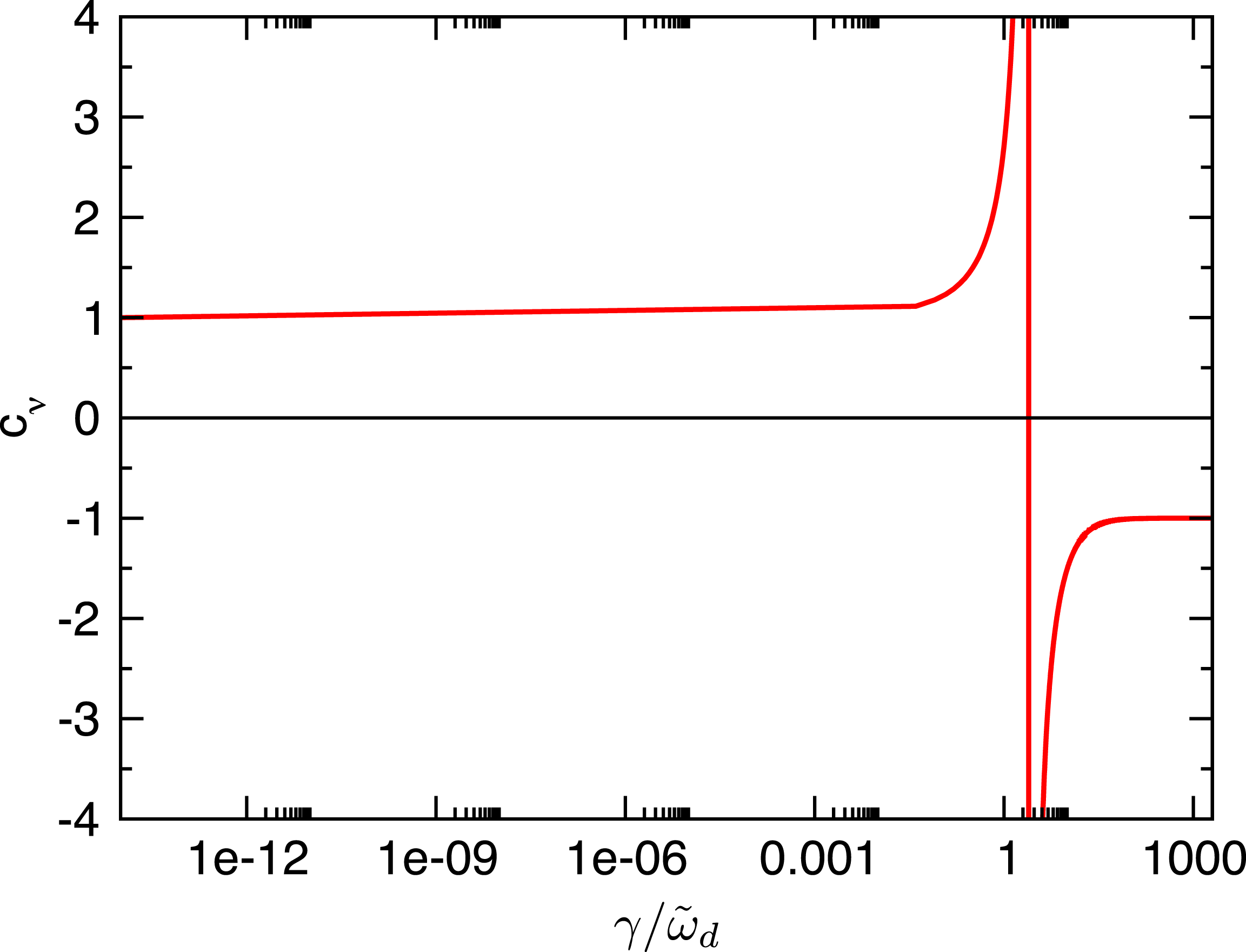
Frequency-dependent coefficient
 $c_{\unicode[STIX]{x1D708}}$
as a function of the growth rate
 $\unicode[STIX]{x1D6FE}$
.

Using the identity (5.11), one can cast the dispersion relation (5.5) into an alternative form that is particularly simple :
 $$\begin{eqnarray}\unicode[STIX]{x1D714}_{T}=c_{\unicode[STIX]{x1D708}}(\unicode[STIX]{x1D701})\unicode[STIX]{x1D714}_{n}+\Big[2-3c_{\unicode[STIX]{x1D708}}(\unicode[STIX]{x1D701})\Big]\tilde{\unicode[STIX]{x1D714}}_{d},\quad c_{\unicode[STIX]{x1D708}}(\unicode[STIX]{x1D701})=\left[\frac{3}{2}-\frac{\overline{Z}_{6}(\unicode[STIX]{x1D701})}{\overline{Z}_{4}(\unicode[STIX]{x1D701})}\right]^{-1}.\end{eqnarray}$$
We stress that this formulation is equivalent to (5.5). Only the algebraic identity (5.11) and no additional assumptions were needed to derive it. The growth rate enters only through the coefficient
 $c_{\unicode[STIX]{x1D708}}(\unicode[STIX]{x1D701})$
which is plotted in figure 8. One sees that the asymptotic values of this coefficient are
 $$\begin{eqnarray}\lim _{\unicode[STIX]{x1D701}\rightarrow 0}c_{\unicode[STIX]{x1D708}}(\unicode[STIX]{x1D701})=1,\quad \lim _{\unicode[STIX]{x1D701}\rightarrow \infty }c_{\unicode[STIX]{x1D708}}(\unicode[STIX]{x1D701})=-1.\end{eqnarray}$$
It is straightforward to recover the stability and singularity boundaries from these values. The crossing point corresponds to the singularity of
 $c_{\unicode[STIX]{x1D708}}(\unicode[STIX]{x1D701})$
, as shown in figure 8.
5.1 Finite Debye length
From the preceding results it can be inferred that
 $k_{\bot }\unicode[STIX]{x1D706}_{D}\rightarrow 0$
is a singular limit. Indeed (4.6) demonstrates the existence of a fluid mode whose growth rate varies inversely with
 $k_{\bot }\unicode[STIX]{x1D706}_{D}$
. Therefore, we will re-examine the point-dipole limit, assuming a finite Debye length. This leads to a resolution of the singularity boundary that was encountered in the case where
 $k_{\bot }\unicode[STIX]{x1D706}_{D}$
is taken to be exactly zero. We return to (5.1):
 $$\begin{eqnarray}\Big(1+k_{\bot }^{2}\unicode[STIX]{x1D706}_{D}^{2}\Big)\unicode[STIX]{x1D719}=\unicode[STIX]{x1D6EC}\int _{0}^{1/B}\frac{B\,\text{d}\unicode[STIX]{x1D706}}{\sqrt{1-\unicode[STIX]{x1D706}B}}\;\bar{\unicode[STIX]{x1D719}},\quad \unicode[STIX]{x1D6EC}=\frac{1}{n_{0}}\int _{0}^{\infty }\frac{\unicode[STIX]{x1D714}^{2}-\overline{\unicode[STIX]{x1D714}}_{d}\unicode[STIX]{x1D714}_{\ast }^{\text{T}}}{\unicode[STIX]{x1D714}^{2}-\overline{\unicode[STIX]{x1D714}}_{d}^{2}}\,f_{0}\,2\unicode[STIX]{x03C0}v^{2}\,\text{d}v.\end{eqnarray}$$
Multiplying this equation with
 $\unicode[STIX]{x1D719}$
and integrating it over the field line
 $\oint \unicode[STIX]{x1D719}\;(\text{d}l/B)\ldots$
, we obtain the energy principle:
 $$\begin{eqnarray}\displaystyle & & \displaystyle \oint \frac{\text{d}l}{B}\,\left[(k_{\bot }\unicode[STIX]{x1D706}_{D})^{2}\unicode[STIX]{x1D719}^{2}+\int _{0}^{1/B}\frac{B\,\text{d}\unicode[STIX]{x1D706}}{\sqrt{1-\unicode[STIX]{x1D706}B}}\Big(\unicode[STIX]{x1D719}-\bar{\unicode[STIX]{x1D719}}\Big)^{2}\right]\nonumber\\ \displaystyle & & \displaystyle \quad =\left(\unicode[STIX]{x1D6EC}-\frac{1}{2}\right)\oint \frac{\text{d}l}{B}\mathop{\int }_{0}^{1/B}\frac{B\,\text{d}\unicode[STIX]{x1D706}}{\sqrt{1-\unicode[STIX]{x1D706}B}}\bar{\unicode[STIX]{x1D719}}^{2}.\end{eqnarray}$$
This relation is general and has been derived without further assumptions other than neglecting the dependence of
 $\overline{\unicode[STIX]{x1D714}}_{d}$
on the pitch angle
 $\unicode[STIX]{x1D706}$
. It is convenient to obtain the stability condition in the fluid limit
 $\unicode[STIX]{x1D714}\rightarrow \infty$
. In this limit
 $$\begin{eqnarray}\unicode[STIX]{x1D6EC}-\frac{1}{2}\approx -\frac{3\,\tilde{\unicode[STIX]{x1D714}}_{d}^{2}}{2\unicode[STIX]{x1D714}^{2}}\left[\frac{\unicode[STIX]{x1D714}_{T}+\unicode[STIX]{x1D714}_{n}}{\tilde{\unicode[STIX]{x1D714}}_{d}}-5\right].\end{eqnarray}$$
This can be reformulated into the stability condition in the fluid limit:
 $$\begin{eqnarray}\displaystyle \unicode[STIX]{x1D714}^{2}=-\frac{\displaystyle 3\tilde{\unicode[STIX]{x1D714}}_{d}^{2}\oint \frac{\text{d}l}{B}\mathop{\int }_{0}^{1/B}\frac{B\,\text{d}\unicode[STIX]{x1D706}}{\sqrt{1-\unicode[STIX]{x1D706}B}}\bar{\unicode[STIX]{x1D719}}^{2}}{\displaystyle 2\oint \frac{\text{d}l}{B}\,\left[(k_{\bot }\unicode[STIX]{x1D706}_{D})^{2}\unicode[STIX]{x1D719}^{2}+\int _{0}^{1/B}\frac{B\,\text{d}\unicode[STIX]{x1D706}}{\sqrt{1-\unicode[STIX]{x1D706}B}}(\unicode[STIX]{x1D719}-\bar{\unicode[STIX]{x1D719}})^{2}\right]}\left(\frac{\unicode[STIX]{x1D714}_{T}+\unicode[STIX]{x1D714}_{n}}{\tilde{\unicode[STIX]{x1D714}}_{d}}-5\right). & & \displaystyle\end{eqnarray}$$
One sees that the plasma is unstable above the singularity line
 $(\unicode[STIX]{x1D714}_{T}+\unicode[STIX]{x1D714}_{n})/\tilde{\unicode[STIX]{x1D714}}_{d}>5$
and the singularity in the growth rate, previously observed for
 $k_{\bot }\unicode[STIX]{x1D706}_{D}=0$
, is removed. Note that a similar fluid-type instability was found in the Z pinch, see (4.9).
Interestingly, the energy principle can also be used to obtain another useful result. It follows from the energy principle that
 $\unicode[STIX]{x1D719}=\overline{\unicode[STIX]{x1D719}}$
if
 $k_{\bot }\unicode[STIX]{x1D706}_{D}=0$
, implying
 $\langle \unicode[STIX]{x1D719}\rangle =\overline{\unicode[STIX]{x1D719}}=\unicode[STIX]{x1D719}$
, i.e.
 $\unicode[STIX]{x2202}\unicode[STIX]{x1D719}/\unicode[STIX]{x2202}l=0$
. It is a consequence of the energy principle (5.18) and the dispersion relation
 $\unicode[STIX]{x1D6EC}=1/2$
, which we have previously shown to hold for
 $k_{\bot }\unicode[STIX]{x1D706}_{D}=0$
, see (5.1). If
 $k_{\bot }\unicode[STIX]{x1D706}_{D}$
is finite, but small, the deviation of
 $\unicode[STIX]{x1D719}$
from its bounce average or field-line average should also be small
 $\unicode[STIX]{x1D719}\approx \langle \unicode[STIX]{x1D719}\rangle \approx \overline{\unicode[STIX]{x1D719}}$
. Introducing the splitting:
 $$\begin{eqnarray}\unicode[STIX]{x1D719}=\langle \unicode[STIX]{x1D719}\rangle +\widetilde{\unicode[STIX]{x1D719}},\quad \left\langle \widetilde{\unicode[STIX]{x1D719}}\right\rangle =0,\quad \widetilde{\unicode[STIX]{x1D719}}\sim O\left(k_{\bot }^{2}\unicode[STIX]{x1D706}_{D}^{2}\right),\end{eqnarray}$$
with
 $\langle \unicode[STIX]{x1D719}\rangle$
denoting the field-line average and
 $\widetilde{\unicode[STIX]{x1D719}}$
being small for
 $k_{\bot }\unicode[STIX]{x1D706}_{D}\ll 1$
, we can write (5.17) in the form:
 $$\begin{eqnarray}(1+k_{\bot }^{2}\unicode[STIX]{x1D706}_{D}^{2})\langle \unicode[STIX]{x1D719}\rangle +\widetilde{\unicode[STIX]{x1D719}}+k_{\bot }^{2}\unicode[STIX]{x1D706}_{D}^{2}\widetilde{\unicode[STIX]{x1D719}}=2\unicode[STIX]{x1D6EC}\langle \unicode[STIX]{x1D719}\rangle +\unicode[STIX]{x1D6EC}\int _{0}^{1/B}\frac{B\,\text{d}\unicode[STIX]{x1D706}}{\sqrt{1-\unicode[STIX]{x1D706}B}}\;\overline{\widetilde{\unicode[STIX]{x1D719}}}.\end{eqnarray}$$
Integrating this equation along the closed field line and taking into account that
 $$\begin{eqnarray}\oint \frac{\text{d}l}{B}\widetilde{\unicode[STIX]{x1D719}}=0,\quad \oint \frac{\text{d}l}{B}\mathop{\int }_{0}^{1/B}\frac{B\,\text{d}\unicode[STIX]{x1D706}}{\sqrt{1-\unicode[STIX]{x1D706}B}}\overline{\widetilde{\unicode[STIX]{x1D719}}}=2\oint \frac{\text{d}l}{B}\;\widetilde{\unicode[STIX]{x1D719}}=0\end{eqnarray}$$
by definition, we obtain the dispersion relation, accurate to the second order:
 $$\begin{eqnarray}\unicode[STIX]{x1D6EC}=\frac{1+\langle k_{\bot }^{2}\unicode[STIX]{x1D706}_{D}^{2}\rangle }{2}+O\left(k_{\bot }^{4}\unicode[STIX]{x1D706}_{D}^{4}\right),\quad \langle k_{\bot }^{2}\unicode[STIX]{x1D706}_{D}^{2}\rangle =\frac{1}{\oint \text{d}l/B}\;\oint \frac{\text{d}l}{B}\;\mathop{k}_{\bot }^{2}\unicode[STIX]{x1D706}_{D}^{2}.\end{eqnarray}$$
In the crossing-point notation (5.12), this dispersion relation becomes
 $$\begin{eqnarray}\frac{\overline{Z}_{4}}{2\unicode[STIX]{x1D701}^{3}}\;\left(\unicode[STIX]{x1D708}-\frac{\unicode[STIX]{x1D70F}}{c_{\unicode[STIX]{x1D708}}}\right)=\langle k_{\bot }^{2}\unicode[STIX]{x1D706}_{D}^{2}\rangle .\end{eqnarray}$$
It is instructive to find the asymptotes of this dispersion relation. For
 $\unicode[STIX]{x1D701}\rightarrow \infty$
 $$\begin{eqnarray}\unicode[STIX]{x1D708}+\unicode[STIX]{x1D70F}=-\frac{4\unicode[STIX]{x1D701}^{4}}{3}\;\left\langle k_{\bot }^{2}\unicode[STIX]{x1D706}_{D}^{2}\right\rangle \quad \Longleftrightarrow \quad \unicode[STIX]{x1D714}^{2}=-\frac{3\,\tilde{\unicode[STIX]{x1D714}}_{d}^{2}}{\langle k_{\bot }^{2}\unicode[STIX]{x1D706}_{D}^{2}\rangle }\;\left[\frac{\unicode[STIX]{x1D714}_{T}+\unicode[STIX]{x1D714}_{n}}{\tilde{\unicode[STIX]{x1D714}}_{d}}-5\right].\end{eqnarray}$$
One sees that plasma is unstable if
 $\unicode[STIX]{x1D714}_{T}+\unicode[STIX]{x1D714}_{n}>5\,\tilde{\unicode[STIX]{x1D714}}_{d}$
, in agreement with (5.20). At the singularity line itself,
 $\unicode[STIX]{x1D714}=0$
which contradicts the condition
 $\unicode[STIX]{x1D701}\gg 1$
, assumed above. This contradiction can be resolved taking higher-order terms in the plasma dispersion function into account. For this sake, we expand the plasma dispersion function (Fried & Conte Reference Fried and Conte1961) as
 $$\begin{eqnarray}\displaystyle & & \displaystyle Z_{0}=\text{i}\sqrt{\unicode[STIX]{x03C0}}e^{-\unicode[STIX]{x1D701}^{2}}-\frac{1}{\sqrt{\unicode[STIX]{x03C0}}}\mathop{\sum }_{n=0}^{\infty }\frac{\unicode[STIX]{x1D6E4}(n+1/2)}{\unicode[STIX]{x1D701}^{2n+1}}\nonumber\\ \displaystyle & & \displaystyle \quad =\text{i}\sqrt{\unicode[STIX]{x03C0}}e^{-\unicode[STIX]{x1D701}^{2}}-\frac{1}{\unicode[STIX]{x1D701}}-\frac{1}{2\unicode[STIX]{x1D701}^{3}}-\frac{3}{4\unicode[STIX]{x1D701}^{5}}-\frac{15}{8\unicode[STIX]{x1D701}^{7}}-\frac{105}{16\unicode[STIX]{x1D701}^{9}}-\frac{945}{32\unicode[STIX]{x1D701}^{11}}.\end{eqnarray}$$
This expansion leads to the dispersion relation:
 $$\begin{eqnarray}\left\langle k_{\bot }^{2}\unicode[STIX]{x1D706}_{D}^{2}\right\rangle =-\frac{3}{4\unicode[STIX]{x1D701}^{4}}\left[(\unicode[STIX]{x1D70F}+\unicode[STIX]{x1D708})+\frac{35}{4\unicode[STIX]{x1D701}^{4}}(3\unicode[STIX]{x1D70F}+\unicode[STIX]{x1D708})\right].\end{eqnarray}$$
At the singularity line
 $\unicode[STIX]{x1D70F}+\unicode[STIX]{x1D708}=0$
. Here, the dispersion relation degenerates to
 $$\begin{eqnarray}\left\langle k_{\bot }^{2}\unicode[STIX]{x1D706}_{D}^{2}\right\rangle =-\frac{105\unicode[STIX]{x1D70F}}{8\unicode[STIX]{x1D701}^{8}}\quad \Longleftrightarrow \quad \unicode[STIX]{x1D714}^{4}=-\unicode[STIX]{x1D70F}\frac{210\tilde{\unicode[STIX]{x1D714}}_{d}^{4}}{\langle k_{\bot }^{2}\unicode[STIX]{x1D706}_{D}^{2}\rangle }.\end{eqnarray}$$
Note that below the crossing point (
 $\unicode[STIX]{x1D70F}<0$
), there is a single unstable root that is purely growing, whereas above the crossing point (
 $\unicode[STIX]{x1D70F}>0$
), there are two unstable solutions with complex frequencies satisfying
 $\text{Im}(\unicode[STIX]{x1D714})=|\text{Re}(\unicode[STIX]{x1D714})|$
.
In the opposite limit
 $\unicode[STIX]{x1D701}\ll 1$
, finite Debye length is less important. It only slightly shifts the stability boundary:
 $$\begin{eqnarray}\unicode[STIX]{x1D708}-\unicode[STIX]{x1D70F}=\left\langle k_{\bot }^{2}\unicode[STIX]{x1D706}_{D}^{2}\right\rangle \quad \Longleftrightarrow \quad \frac{\unicode[STIX]{x1D714}_{n}-\unicode[STIX]{x1D714}_{T}}{\tilde{\unicode[STIX]{x1D714}}_{d}}=1+\left\langle k_{\bot }^{2}\unicode[STIX]{x1D706}_{D}^{2}\right\rangle .\end{eqnarray}$$
Summarising, taking finite Debye length into account resolves the singularity in the growth rate appearing in figure 7. Instead one finds at the singularity boundary that the mode is purely growing (
 $\text{Re}[\unicode[STIX]{x1D714}]=0$
) below the crossing point and has finite frequency and growth rate above the crossing point. The plasma is thus stable only if
 $\unicode[STIX]{x1D714}_{n}-\unicode[STIX]{x1D714}_{T}<\tilde{\unicode[STIX]{x1D714}}_{d}$
and
 $\unicode[STIX]{x1D714}_{n}+\unicode[STIX]{x1D714}_{T}<5\,\tilde{\unicode[STIX]{x1D714}}_{d}$
are both satisfied (i.e. stability is only observed in the left triangular region of figure 7). This clarifies the role of the two stability lines identified by Helander (Reference Helander2014) and Helander & Connor (Reference Helander and Connor2016). Note that the point-dipole (figure 7) and Z-pinch (figure 5) stability diagrams are similar, with the main difference being simply the location of the crossing point of the stability lines.
6 Conclusions
In this paper, we have studied the drift-kinetic stability of a pair plasma, of equal positron and electron temperature and density, confined by a dipole magnetic field. The Z-pinch and point-dipole limits have both been considered, and the resulting dispersion relations have been derived, solved, and compared. We have found electrostatic instabilities in pure pair plasmas driven by the magnetic curvature, temperature and density gradients. In point-dipole geometry, when the Debye length is taken to be exactly zero, we have found that instabilities exist for the parameters in the domain bounded by (5.6) and (5.7). Their growth rate decreases towards the stability boundary defined by (5.6), and increases towards the singularity boundary defined by (5.7). Visually, this is seen in figure 6 from the colour palette and in figure 7 as an increase in the density of the contours of constant growth rate. The singularity can be resolved taking a small but finite Debye length into account. This is associated with a fluid-type mode that is absent if
 $k_{\bot }\unicode[STIX]{x1D706}_{D}=0$
exactly. In the Z-pinch limit, the stability diagram found is similar. With these observations, figures 5, 6 and 7 describe rather thoroughly the drift-kinetic stability of pair plasmas in dipole geometry. We thereby clarify the role of the stability lines in parameter space, and conclude that both density and temperature gradients can drive instability, but that absolute stability is obtained within the left-most triangular region of figures 5 and 7. We note that there is also a smaller region contained within this linearly stable region, in which Helander (Reference Helander2017) has shown that stability also holds nonlinearly. In the Z-pinch geometry, we have treated the Landau damping problem with a novel integration contour, and found exponential and algebraic damping solutions related to the drift particle motion. The existence of such unstable modes is a collective effect that can provide the background turbulence needed for an inward particle pinch (Isichenko et al.
Reference Isichenko, Gruzinov, Diamond and Yushmanov1996; Kobayashi et al.
Reference Kobayashi, Rogers and Dorland2010). Such a pinch could be very helpful for pair plasma creation. We plan to address this with a gyrokinetic code in future.
Finally, we note that our findings, especially the analysis of stability boundaries, are strongly reminiscent of previous studies of electron–ion plasmas in dipole and Z-pinch geometries, leading us to associate the resonant stability boundary with the entropy mode (Simakov et al.
Reference Simakov, Catto and Hastie2001; Ricci et al.
Reference Ricci, Rogers, Dorland and Barnes2006b
), and the fluid stability (singularity) boundary with the MHD-like electrostatic interchange mode (Simakov et al.
Reference Simakov, Catto and Hastie2001; Kesner et al.
Reference Kesner, Simakov, Garnier, Catto, Hastie, Krasheninnikov, Mauel, Pedersen and Ramos2001). However, we note that the correspondence is inexact: the ion Larmor radius
 $\unicode[STIX]{x1D70C}_{i}$
in electron–ion plasmas contributes in a similar way to the dispersion relation as the Debye length does here, but only in the limit
 $k_{\bot }\unicode[STIX]{x1D70C}_{i}\ll 1$
, so that the analysis diverges as
 $k_{\bot }\unicode[STIX]{x1D70C}_{i}$
becomes finite; note that the entropy mode reaches its largest growth rate at
 $k_{\bot }\unicode[STIX]{x1D70C}_{i}\gtrsim 1$
(Ricci et al.
Reference Ricci, Rogers, Dorland and Barnes2006b
). On the other hand, when
 $k_{\bot }\unicode[STIX]{x1D70C}_{i}$
is small but non-zero, in the non-resonant limit, the interchange mode obtained is quite close to the fluid mode that we find, with the dispersion relations having identical form in the collisionless limit. However, note this dispersion relation becomes invalid for the interchange mode when
 $k_{\bot }\unicode[STIX]{x1D70C}_{i}\sim 1$
, while, for our case, it can still correctly describe the mode when
 $k_{\bot }\unicode[STIX]{x1D706}_{D}\sim 1$
(at sufficiently large drive). We note that despite the physical and mathematical differences with previous studies of electron–ion plasmas, our results would be directly applicable to a certain class of such plasmas, namely those with equal ion and electron temperatures,
 $k_{\bot }^{-1}\sim \unicode[STIX]{x1D706}_{D}\gg \unicode[STIX]{x1D70C}_{i}$
, at frequencies below the ion bounce frequency.
Acknowledgements
We acknowledge Thomas Sunn Pedersen and PAX/APEX experiment team for their interest to our work. We thank Alessandro Zocco for useful comments and suggestions.