1 Introduction
Slightly blunted cones are commonly understood to delay hypersonic boundary-layer transition when compared to sharp cones (Malik, Spall & Chang Reference Malik, Spall and Chang1990). This phenomenon is consistently seen in wind tunnels as well as in free flight. In many reentry vehicles, some nose bluntness is required to not only delay transition, but to mitigate high heat loads that would be present for sharp leading edges.
Wind tunnel tests, most prominently those of Stetson & Rushton (Reference Stetson and Rushton1967) and Softley (Reference Softley1968), have been used to analyse the transition delay due to nose bluntness. From these tests and subsequent analyses, it is commonly understood that blunting a cone damps the second mode which delays transition. These tests were for low-enthalpy flows adequately modelled with an assumption of a perfect gas. However, the tests do not reproduce all flow conditions similar to free flight. This is due in part to the low temperatures behind the bow shock which do not allow for any significant amount of chemical reaction. In free flight, an increase in nose bluntness corresponds to an increase in real-gas effects which are not found in low-enthalpy wind tunnels. Accordingly, multiple studies (Chang, Vinh & Malik Reference Chang, Vinh and Malik1997; Malik Reference Malik2003; Mortensen & Zhong Reference Mortensen and Zhong2014) have shown that in high-enthalpy flows there can be a marked change in behaviour of modal instability based on the model used for the gas, i.e. a real-gas or perfect-gas model. Therefore, it is important to understand the similarities, or differences, in the physical mechanisms that cause transition delay for blunt cones in high- and low-enthalpy flows.
For a hypersonic boundary layer over a sharp cone at zero angle-of-attack, the most unstable boundary-layer mode has been shown to be the second mode. The second mode was originally found by Mack (Reference Mack1969) and has been studied extensively ever since. He also showed that there exists neutral supersonic waves that transfer energy to infinity, i.e. away from the wall. These waves are called ‘supersonic’ because the phase velocity of the wave is supersonic relative to the flow at the edge of the boundary layer. This corresponds to
 $c_{r}<1-1/M_{e}$
where
 $c_{r}$
is the phase velocity and
 $M_{e}$
is the Mach number at the edge of the boundary layer.
In Mack (Reference Mack1987), it was shown that for a Mach 5.8 flow over a flat plate these supersonic waves were unstable when
 $T_{w}/T_{r}<0.25$
where
 $T_{w}$
is the wall temperature and
 $T_{r}$
is the recovery temperature. Following research from Chang et al. (Reference Chang, Vinh and Malik1997) showed that including chemical reactions in hypersonic boundary layers over cones can destabilize these supersonic waves. Recently, Bitter & Shepherd (Reference Bitter and Shepherd2015) showed that supersonic waves were unstable for high Mach number and high-enthalpy flows over cones where the walls are highly cooled. One example of such a flow would be one produced by a high-enthalpy impulse facility and another a flow around a slender vehicle reentering the Earth’s atmosphere. However, none of the previous research investigated the effects of nose bluntness on the supersonic mode as the focus was on relatively sharp geometries.
There are a few tools used to analyse boundary-layer instability. They fall broadly into two categories: theoretical and direct. A common theoretical treatment of boundary-layer instability would be linear stability theory (LST), or parabolized stability equations (PSE). These methods rely on the assumption that the flow can be decomposed into mean and fluctuating components where the fluctuating component is wave-like. They can be used to quickly analyse a flow field once the mean-flow solution is complete. The second category is the direct method of simulating flow disturbances and is commonly called direct numerical simulation (DNS). This method computes the entire flow field disturbance structure without the simplifying assumptions used in the theoretical approaches. However, this method can prove quite time consuming, even with massively parallel computing systems, so it is often used for only a small number of cases. Here, a combination of LST and DNS will be used to analyse multiple flow fields with varying nose radii.
The goal of this paper is to better understand the physical mechanisms leading to boundary-layer transition for vehicles similar to blunt cones at realistic reentry trajectory points. One of these mechanisms is the supersonic mode and its characteristics will be studied in detail. To elucidate issues due to nose blunting, simulations are run at a single trajectory point while varying the nose radius. A thermochemical non-equilibrium flow model is used to capture the real-gas effects that occur for reentry flows with high Mach numbers. The important boundary-layer modes for each case will be analysed using LST and then a single case will be analysed in-depth using DNS.
This paper will start with an explanation of the governing equations for the thermochemical non-equilibrium model in § 2. Then a brief explanation of the computational methods used is given in § 3. Following this will be an explanation of the results using LST and DNS in § 4 and then conclusions in § 5.
2 Governing equations
The governing equations are the Navier–Stokes equations including thermal and chemical non-equilibrium effects. To model thermal non-equilibrium, two temperatures are used. One temperature
 $T$
represents translation–rotational energy and the other temperature
 $T_{V}$
represents vibrational energy. A five-species model (
 $\text{N}_{2}$
,
 $\text{O}_{2}$
, NO, N and O) is used to simulate chemical non-equilibrium in air. The conservative three-dimensional Navier–Stokes equations consist of five-species mass conservation equations, three momentum conservation equations, the vibration energy conservation equation and the total energy conservation equation. Written in vector form the governing equations are
 $$\begin{eqnarray}\frac{\unicode[STIX]{x2202}U}{\unicode[STIX]{x2202}t}+\frac{\unicode[STIX]{x2202}F_{j}}{\unicode[STIX]{x2202}x_{j}}+\frac{\unicode[STIX]{x2202}G_{j}}{\unicode[STIX]{x2202}x_{j}}=W,\end{eqnarray}$$
where
 $t$
is the simulation time and
 $x_{j}$
are the simulation coordinates.
 $U$
is the state vector of conserved quantities defined by
 $$\begin{eqnarray}U^{\text{T}}=[\unicode[STIX]{x1D70C}_{1},\unicode[STIX]{x1D70C}_{2},\ldots ,\unicode[STIX]{x1D70C}_{ns},\unicode[STIX]{x1D70C}u_{1},\unicode[STIX]{x1D70C}u_{2},\unicode[STIX]{x1D70C}u_{3},\unicode[STIX]{x1D70C}e,\unicode[STIX]{x1D70C}e_{v}]\end{eqnarray}$$
and
 $W$
is the source terms defined by
 $$\begin{eqnarray}W^{\text{T}}=\left[\unicode[STIX]{x1D714}_{1},\unicode[STIX]{x1D714}_{2},\ldots ,\unicode[STIX]{x1D714}_{ns},0,0,0,0,\mathop{\sum }_{s=1}^{\mathit{nms}}(Q_{T-V,s}+\unicode[STIX]{x1D714}_{s}e_{v,s})\right],\end{eqnarray}$$
where
 $\unicode[STIX]{x1D70C}_{s}$
is the species density,
 $\unicode[STIX]{x1D70C}$
is the mixture density,
 $u_{j}$
is the velocity in the
 $j$
th direction,
 $e_{v,s}$
is the specific vibration energy of species
 $s$
,
 $\unicode[STIX]{x1D714}_{s}$
is the rate of production of species
 $s$
and
 $Q_{T-V,s}$
is the species vibration energy transfer rate. The number of species is denoted by
 $ns$
and the number of molecular species by
 $nms$
. The inviscid and viscous fluxes are
 $F_{j}$
and
 $G_{j}$
, respectively, and are defined by
 $$\begin{eqnarray}F_{j}=\left[\begin{array}{@{}c@{}}\unicode[STIX]{x1D70C}_{1}u_{j}\\ \vdots \\ \unicode[STIX]{x1D70C}_{\mathit{ns }}u_{j}\\ \unicode[STIX]{x1D70C}u_{1}u_{j}+p\unicode[STIX]{x1D6FF}_{1j}\\ \unicode[STIX]{x1D70C}u_{2}u_{j}+p\unicode[STIX]{x1D6FF}_{2j}\\ \unicode[STIX]{x1D70C}u_{3}u_{j}+p\unicode[STIX]{x1D6FF}_{3j}\\ \left(\unicode[STIX]{x1D70C}e+p\right)u_{j}\\ \unicode[STIX]{x1D70C}e_{v}u_{j}\end{array}\right],\quad G_{j}=\left[\begin{array}{@{}c@{}}\unicode[STIX]{x1D70C}_{1}v_{1j}\\ \vdots \\ \unicode[STIX]{x1D70C}_{\mathit{ns }}v_{\mathit{ns }j}\\ \unicode[STIX]{x1D70F}_{1j}\\ \unicode[STIX]{x1D70F}_{2j}\\ \unicode[STIX]{x1D70F}_{3j}\\ -u_{i}\unicode[STIX]{x1D70F}_{ij}-k_{T}{\displaystyle \frac{\unicode[STIX]{x2202}T}{\unicode[STIX]{x2202}x_{j}}}-k_{V}{\displaystyle \frac{\unicode[STIX]{x2202}T_{V}}{\unicode[STIX]{x2202}x_{j}}}+\displaystyle \mathop{\sum }_{s=1}^{\mathit{nms}}\unicode[STIX]{x1D70C}_{s}h_{s}v_{sj}\\ -k_{V}{\displaystyle \frac{\unicode[STIX]{x2202}T_{V}}{\unicode[STIX]{x2202}x_{j}}}+\displaystyle \mathop{\sum }_{s=1}^{\mathit{nms}}\unicode[STIX]{x1D70C}_{s}e_{v,s}v_{sj}\end{array}\right],\end{eqnarray}$$
where
 $p$
is the pressure,
 $k_{T}$
is the translation–rotation thermal conductivity,
 $k_{V}$
is the vibration thermal conductivity,
 $\unicode[STIX]{x1D6FF}_{ij}$
is the Kronecker delta,
 $v_{sj}$
is the species diffusion velocity and
 $$\begin{eqnarray}\unicode[STIX]{x1D70F}_{ij}=\unicode[STIX]{x1D707}\left(\frac{\unicode[STIX]{x2202}u_{i}}{\unicode[STIX]{x2202}x_{j}}+\frac{\unicode[STIX]{x2202}u_{j}}{\unicode[STIX]{x2202}x_{i}}\right)-\frac{2}{3}\unicode[STIX]{x1D707}\frac{\unicode[STIX]{x2202}u_{k}}{\unicode[STIX]{x2202}x_{k}}\unicode[STIX]{x1D6FF}_{ij}\end{eqnarray}$$
is the viscous stress. The total energy per unit volume
 $\unicode[STIX]{x1D70C}e$
is defined by
 $$\begin{eqnarray}\unicode[STIX]{x1D70C}e=\mathop{\sum }_{s=1}^{\mathit{ns}}\unicode[STIX]{x1D70C}_{s}c_{v,s}T+\unicode[STIX]{x1D70C}e_{v}+\frac{1}{2}\unicode[STIX]{x1D70C}u_{i}u_{i}+\mathop{\sum }_{s=1}^{\mathit{ns}}\unicode[STIX]{x1D70C}_{s}h_{s}^{o},\end{eqnarray}$$
where
 $h_{s}^{o}$
is the heat of formation of species
 $s$
and
 $c_{v,s}$
is the species translation–rotation specific heat at constant volume defined as
 $$\begin{eqnarray}c_{v,s}=\left\{\begin{array}{@{}ll@{}}{\displaystyle \frac{5}{2}}{\displaystyle \frac{R}{M_{s}}},\quad & s=1,2,\ldots ,\mathit{nms},\\ {\displaystyle \frac{3}{2}}{\displaystyle \frac{R}{M_{s}}},\quad & s=\mathit{nms}+1,\ldots ,\mathit{ns},\end{array}\right.\end{eqnarray}$$
where
 $R$
is the universal gas constant and
 $M_{s}$
is the species molecular weight. The vibration energy per unit volume
 $\unicode[STIX]{x1D70C}e_{v}$
is defined as
 $$\begin{eqnarray}\unicode[STIX]{x1D70C}e_{v}=\mathop{\sum }_{s=1}^{\mathit{nms}}\unicode[STIX]{x1D70C}_{s}e_{v,s}=\mathop{\sum }_{s=1}^{\mathit{nms}}\unicode[STIX]{x1D70C}_{s}\frac{R}{M_{s}}\frac{\unicode[STIX]{x1D703}_{v,s}}{\exp (\unicode[STIX]{x1D703}_{v,s}/T_{V})-1},\end{eqnarray}$$
where
 $\unicode[STIX]{x1D703}_{v,s}$
refers to the characteristic temperature of each vibrational mode. The characteristic vibration temperatures are taken from Park (Reference Park1990).
To model chemical non-equilibrium, three dissociation reactions and three exchange reactions are used. Each reaction is governed by a forward
 $k_{f}$
and backward
 $k_{b}$
reaction rate determined from
 $$\begin{eqnarray}\displaystyle & k_{f}=C_{f}T_{a}^{\unicode[STIX]{x1D702}}\text{e}^{(-\unicode[STIX]{x1D703}_{d}/T_{a})}, & \displaystyle\end{eqnarray}$$
 $$\begin{eqnarray}\displaystyle & k_{b}=k_{f}/K_{eq}, & \displaystyle\end{eqnarray}$$
where all forward reaction-rate constants are taken from Park (Reference Park1990). The equilibrium coefficient
 $K_{eq}$
is determined using
 $$\begin{eqnarray}K_{eq}=A_{0}\exp \left(\frac{A_{1}}{Z}+A_{2}+A_{3}\ln (Z)+A_{4}Z+A_{5}Z^{2}\right),\end{eqnarray}$$
where
 $Z=10000T^{-1}$
. This is a curve fit to experimental data from Park (Reference Park1990).
To calculate the source term in the vibration energy equation representing the exchange of energy between the translational–rotational and vibrational energies, the Landau–Teller expression is used
 $$\begin{eqnarray}Q_{T-V,s}=\unicode[STIX]{x1D70C}_{s}\frac{e_{v,s}(T)-e_{v,s}(T_{V})}{\langle \unicode[STIX]{x1D70F}_{s}\rangle +\;\unicode[STIX]{x1D70F}_{cs}},\end{eqnarray}$$
where
 $\langle \unicode[STIX]{x1D70F}_{s}\rangle$
is the Landau–Teller vibration relaxation time given by Lee (Reference Lee and Nelson1985). The term
 $\unicode[STIX]{x1D70F}_{cs}$
is from Park (Reference Park1990) and is used to more accurately model the relaxation time in areas of high temperatures occurring just downstream of the bow shock.
The viscosity of each species
 $\unicode[STIX]{x1D707}_{s}$
is computed using a Blottner curve fit shown in (2.13). The coefficients are obtained from Blottner, Johnson & Ellis (Reference Blottner, Johnson and Ellis1971). The mixture viscosity
 $\unicode[STIX]{x1D707}$
is then found using each species viscosity from a mixing rule obtained from Wilke (Reference Wilke1950) (equation (2.14)). The total heat conductivities for each energy mode are computed in a similar fashion to viscosity. The diffusion velocity is calculated using Fick’s law and a constant Schmidt number of 0.5.
 $$\begin{eqnarray}\displaystyle & \displaystyle \unicode[STIX]{x1D707}_{s}=0.1\exp [(A_{s}^{\unicode[STIX]{x1D707}}\ln (T)+B_{s}^{\unicode[STIX]{x1D707}})\ln (T)+C_{s}^{\unicode[STIX]{x1D707}}], & \displaystyle\end{eqnarray}$$
 $$\begin{eqnarray}\displaystyle & \displaystyle \unicode[STIX]{x1D707}=\mathop{\sum }_{s=1}^{\mathit{ns}}\frac{X_{s}\unicode[STIX]{x1D707}_{s}}{\unicode[STIX]{x1D719}_{s}}. & \displaystyle\end{eqnarray}$$
3 Computational methods
The high-order DNS code described by Mortensen & Zhong (Reference Mortensen and Zhong2014) is used to compute the steady and unsteady flow fields. This code is based on a shock-fitting formulation originally described by Zhong (Reference Zhong1998) that uses a finite-difference scheme with fifth-order upwinded stencils and explicit time integration. The finite-difference stencils were designed to minimize numerical dissipation so unsteady disturbances with small amplitudes could be simulated accurately. Shock fitting in this context means that the bow shock is treated as a boundary in the numerical simulation where the boundary conditions at the shock are derived from the Rankine–Hugoniot jump conditions.
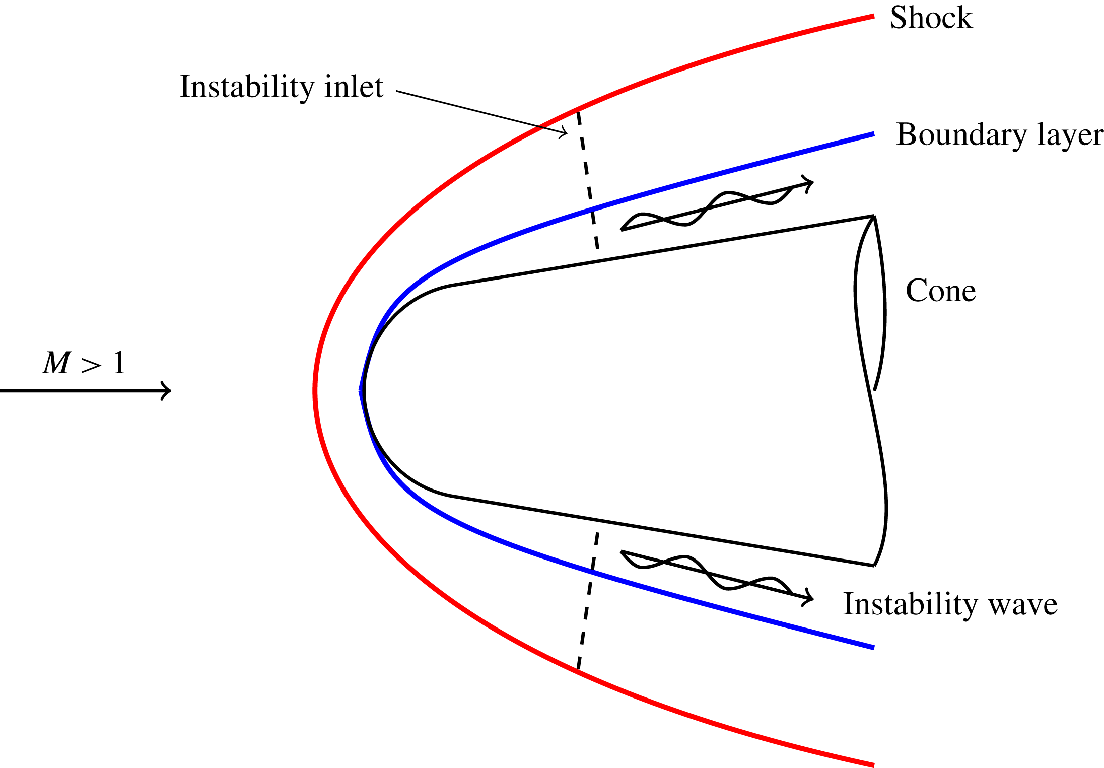
Schematic of a DNS for hypersonic flow over a blunt cone. Perturbation imposed at a single streamwise location in the wall-normal direction.

For a DNS, a laminar mean-flow simulation is run and the solution is stored. Next, a perturbation is imposed on the mean flow and it is directly simulated as it passes through the computational domain. Figure 1 shows the simulated domain for a cone where
 $M$
is the Mach number. Note that the dimensions are not to scale. Here, the perturbations imposed on the DNS are modes from linear stability theory and are imposed at a single streamwise location. The perturbations are simulated for a long enough time that they have become periodic. Once this occurs, a fast Fourier transform (FFT) is performed at each point in the flow. This decomposes the unsteady flow field into an amplitude and phase for each frequency component giving
 $$\begin{eqnarray}q^{\prime }(x,y,z,t)=\unicode[STIX]{x0394}q(x,y,z)\exp [\text{i}(\unicode[STIX]{x1D713}(x,y,z)-2\unicode[STIX]{x03C0}ft)],\end{eqnarray}$$
where
 $q$
is some flow variable,
 $q^{\prime }$
is the unsteady component,
 $\unicode[STIX]{x0394}q$
is the amplitude,
 $\unicode[STIX]{x1D713}$
is the phase angle and
 $f$
is the frequency. Here, only one mode is simulated at a time which means only one frequency is imposed. However, an FFT helps to separate out the mean-flow distortion – zero frequency component – and can show nonlinearity of disturbances if the amplitude of higher harmonics begins to grow.
The LST code described by Mortensen & Zhong (Reference Mortensen and Zhong2016) is used to analyse the steady flow computed by the DNS code. The LST equations are derived from the non-conservative form of the governing equations for thermochemical non-equilibrium flow where the instantaneous flow consists of mean and fluctuating components
 $q=\bar{q}+q^{\prime }$
. Again,
 $q$
represents any flow variable such as velocity, species density, etc. The instantaneous flow is then substituted into the governing equations where the steady flow is assumed to be a function of the wall-normal coordinate
 $y$
only, i.e.
 $\bar{q}(x,y,z)\approx \bar{q}(y)$
. Also, the flow disturbances are assumed to be small, i.e. linear so modal interactions are neglected. The perturbations are then assumed to be in the form of a normal mode described by
 $$\begin{eqnarray}q^{\prime }(x,y,z)=\hat{q}(y)\exp [\text{i}(\unicode[STIX]{x1D6FC}x+\unicode[STIX]{x1D6FD}z-2\unicode[STIX]{x03C0}ft)],\end{eqnarray}$$
where
 $\unicode[STIX]{x1D6FC}$
and
 $\unicode[STIX]{x1D6FD}$
are the wavenumbers. Here,
 $f$
and
 $\unicode[STIX]{x1D6FD}$
are assumed to be real and the wavenumber
 $\unicode[STIX]{x1D6FC}$
is assumed to be complex which means the modes grow in space, rather than time. A negative imaginary part of the wavenumber
 $\unicode[STIX]{x1D6FC}$
results in disturbance growth while a positive value results in disturbance decay. Often LST results are put in terms of the growth rate which is defined as
 $-\unicode[STIX]{x1D6FC}_{i}$
. The phase velocity of a mode is
 $\unicode[STIX]{x1D714}/\unicode[STIX]{x1D6FC}_{r}$
and is non-dimensionalized here by the wall-tangent velocity directly downstream of the shock. A complete derivation of the thermochemical non-equilibrium LST equations is described by Mortensen (Reference Mortensen2016).
Boundary conditions for the wave modes are required at the wall and in the free stream. At the wall, the boundary conditions are
 $T^{\prime }=0$
from the energy equation,
 $T_{V}^{\prime }=T^{\prime }$
from thermal equilibrium,
 $u^{\prime },v^{\prime },w^{\prime }=0$
from the no-slip condition and
 $\unicode[STIX]{x2202}c_{s}^{\prime }/\unicode[STIX]{x2202}n=0$
from a non-catalytic wall. Lastly, a linearized pressure extrapolation condition is used in place of one of the linearized non-catalytic equations to account for the incoming characteristic at the surface. Since the mean-flow solutions are from a shock-fitting code, the free-stream boundary of the mean flow is the bow shock. It is convenient then to use the bow shock to bound the wave modes as well. For the wave modes, the boundary conditions at the bow shock are the linearized Rankine–Hugoniot conditions.
The derivation of the linearized equations is similar to that of Hudson (Reference Hudson1996), except that the species velocities are not found from a first-order truncation of a Taylor series expansion. Rather, the usual prescription of substituting a mean and fluctuating component and then linearizing is followed. This has been shown to not significantly affect the results (Mortensen Reference Mortensen2016). The main difference is in the treatment of the boundary conditions. In Hudson (Reference Hudson1996), the fact that the pressure derivative normal to the surface is zero is included implicitly in the boundary conditions. This has been shown to make the solution first-order accurate (Mortensen & Zhong Reference Mortensen and Zhong2016). Here, the pressure boundary condition is a linearized extrapolation of pressure. It is included explicitly and allows the solution to be of arbitrary order.
Note that, the real and imaginary parts of
 $\unicode[STIX]{x1D6FC}$
can be compared to DNS results by taking appropriate derivatives of (3.1) and (3.2). Also, the eigenfunction may be compared to the instantaneous DNS results after it has been appropriately scaled. A comparison shows how well the modes from theory match those from direct simulation of the governing equations without simplifying assumptions.
LST gives information about which disturbance frequencies are unstable and the corresponding growth rates of those frequencies, but there is no information on the amplitude of the incoming disturbance. To estimate boundary-layer transition using LST, the
 $\text{e}^{N}$
transition criterion is used which is defined as
 $$\begin{eqnarray}\text{e}^{N}=\frac{A}{A_{0}}=\exp \left(-\int _{s_{0}}^{s}\unicode[STIX]{x1D6FC}_{i}\,\text{d}x\right),\end{eqnarray}$$
where
 $A$
is the integrated disturbance amplitude,
 $A_{0}$
is the initial amplitude, and
 $s_{0}$
is the streamwise location where the disturbance first becomes unstable. The integration is performed for a constant frequency
 $f$
. The
 $N$
factor is specifically the exponent of
 $\text{e}^{N}$
. In-flight transition
 $N$
factors are commonly understood to be approximately ten. Malik (Reference Malik2003) showed that 9.5 and 11.2 correlated with transition onset for two high Mach number flight tests. In noisy ground test facilities the transition
 $N$
factor is usually much lower and is typically close to five.
4 Results
Multiple shock-fitting simulations for a flow in thermochemical non-equilibrium are run for a blunt cone with a
 $8^{\circ }$
half-angle at a zero degree angle-of-attack. The free-stream conditions are
 $M=20$
,
 $T=222.5~\text{K}$
,
 $p=2188~\text{N}~\text{m}^{-2}$
,
 $c_{N_{2}}=0.78$
and
 $c_{O_{2}}=0.22$
. The free-stream stagnation enthalpy is
 $18.2~\text{MJ}~\text{kg}^{-1}$
and the free-stream unit Reynolds number, defined as
 $Re_{u}=\unicode[STIX]{x1D70C}u_{\infty }/\unicode[STIX]{x1D707}_{\infty }$
, is
 $14.0\times 10^{6}~\text{m}^{-1}$
. These conditions correspond to an altitude of 26 km (85 kft) and are chosen as generic conditions where transition from laminar-to-turbulent flow would likely be an important factor in vehicle flight dynamics for slender reentry vehicles. Multiple steady simulations for the same free-stream conditions are run while the nose radius is varied. Case 1 has a nose radius of
 $r_{n}=1.1~\text{mm}$
. Cases 2–5 have nose radii of 8.9 mm, 35.6 mm, 71.2 mm and 284.8 mm, respectively. Case 1 is used in place of a perfectly sharp cone.
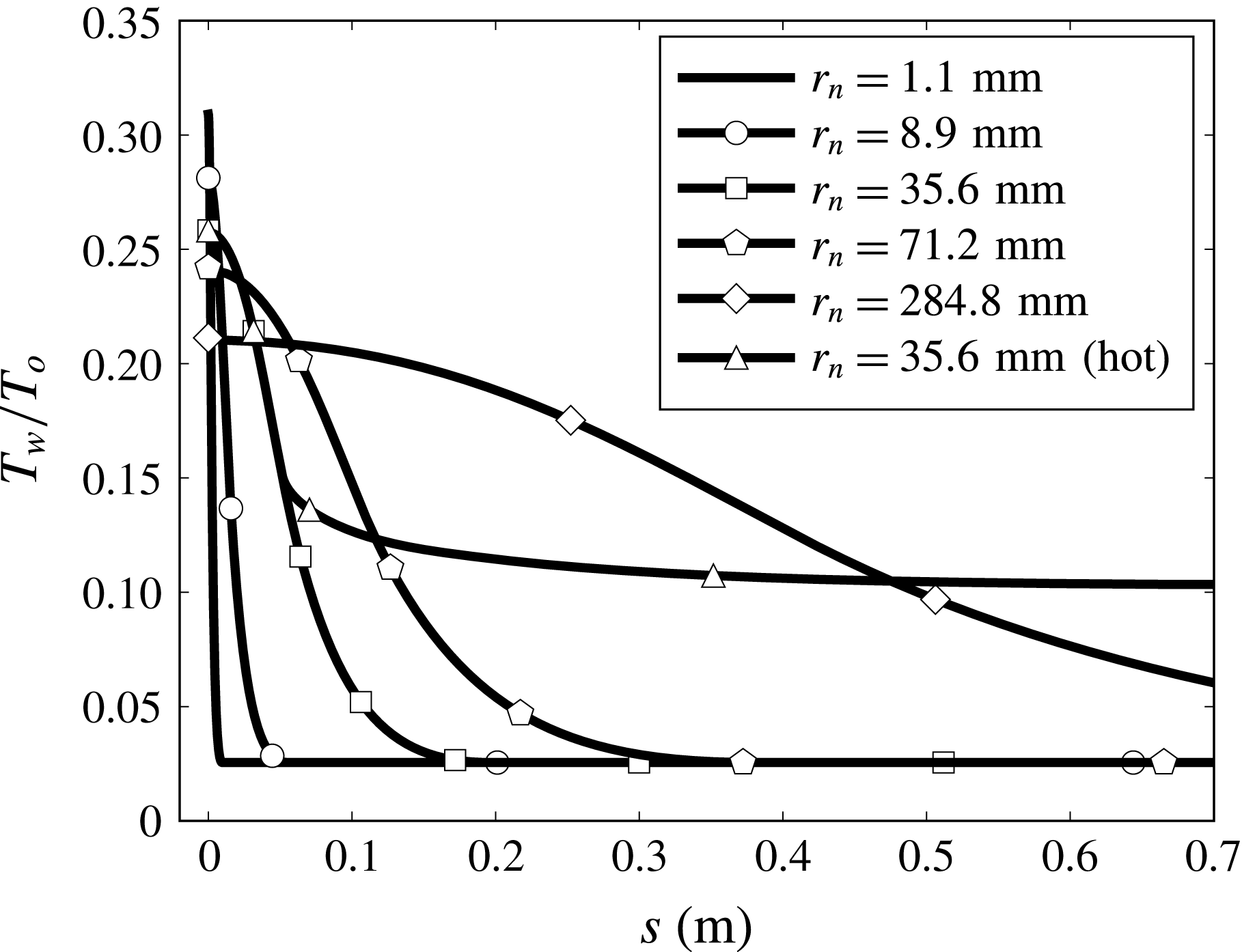
The wall boundary conditions for each simulation are no slip for each velocity, non-catalytic for each chemical species, equilibrium for vibration temperature and radiative wall for translation–rotation temperature. Using a radiative wall condition for the entire cone frustum can give wall temperatures that are too high. On the cone frustum, the temperatures were exponentially lowered to 460 K to more accurately model in-flight vehicle temperatures. Figure 2 shows the wall temperature for each case.
 $T_{w}$
is the local wall temperature,
 $T_{o}$
is the stagnation temperature and hot denotes a case where the radiative wall boundary condition is used throughout. For the second mode, a lower wall temperature (wall cooling) is destabilizing (Mack Reference Mack1984). Therefore, if the radiative wall condition is used over the entire cone frustum, the wall temperature may be too high and the boundary layer will be artificially stabilized.
Comparison of the wall temperature for each case where the word hot denotes the use of the radiative wall condition over the entire surface.

These wall boundary conditions are a simplification of the surface of a real reentry vehicle. A real vehicle would likely have an ablating nose cone that would introduce new chemical species, often containing carbon, into the flow due to mass loss at the surface. Ablation would also change the surface shape as well as create surface roughness. In Mortensen & Zhong (Reference Mortensen and Zhong2016), a high-enthalpy flow over a cone with an ablating surface was modelled in a DNS code which showed mass addition destabilized the second mode. There was no attempt to model roughness and it is still an open question as to how roughness due to ablation affects the transition process. Here, ablation effects are neglected to simplify the analysis but the instabilities present away from the ablating nose cone would likely be the same whether ablation effects are included or not.
A grid resolution study was performed and it was found that 640 points were required in the wall-normal direction to get accurate boundary-layer profiles for the LST solver and unsteady DNS. The streamwise grid for the unsteady DNS was set to resolve the wavenumber of the imposed modes. This grid is significantly denser than a grid required to obtain only an accurate mean-flow solution.
4.1 Mean flow
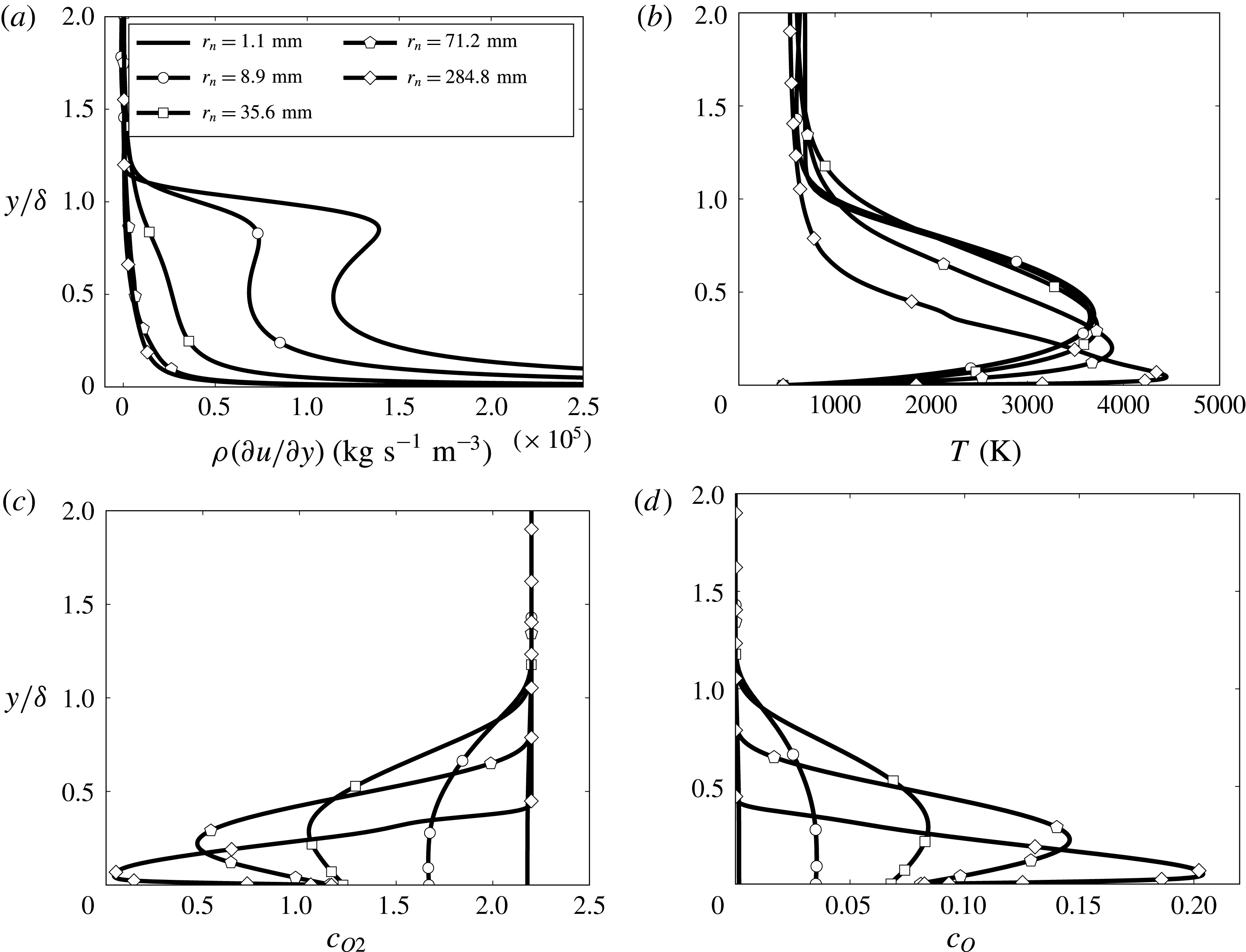
Figure 3 shows a comparison of boundary-layer profiles for cases 1–5 where
 $\unicode[STIX]{x1D6FF}$
is the height of the velocity boundary layer and
 $c_{s}$
is the mass fraction of species
 $s$
. The streamwise locations for comparison are 0.82 m, 1.56 m, 4.57 m, 6.44 m and 11.03 m. These locations correspond to an
 $N$
factor of ten for each case which is an estimate of transition. For cases 1 and 2, the growth of the second mode causes
 $N=10$
and for cases 3–5 growth of the supersonic mode causes
 $N=10$
. At each of these locations the wall temperature has reached the constant value of 460 K.
Boundary-layer profile comparison of (a) angular momentum, (b) translational–rotational temperature, (c) mass fraction of oxygen and (d) mass fraction of atomic oxygen at the streamwise location where
 $N=10$
.

For a blunt cone, there is an entropy layer that is produced due to the curvature of the bow shock. For sharp geometries similar to case 1, the entropy layer is quickly swallowed by the boundary layer before transition occurs. As the nose radius increases, it takes longer for the entropy layer to be swallowed. The ratio of streamwise location in figure 3 to entropy layer swallowing length for cases 1–5 is 4.17, 0.50, 0.23, 0.13 and 0.03. This entropy layer tends to round out the velocity profile and moves the generalized inflection point towards the wall. The generalized inflection point is the local maximum of the product of density and vorticity, i.e. the angular momentum. The importance of the generalized inflection point was shown by Lees & Lin (Reference Lees and Lin1946) when they determined a stability criterion for inviscid instabilities in compressible boundary layers.
Figure 3(a) shows the distribution of angular momentum in the boundary layer. There is a clear maximum near the boundary-layer edge for the smallest nose radius in case 1. As the nose radius increases in case 2, the generalized inflection point moves towards the wall and the amplitude of the angular momentum at the generalized inflection point decreases. There is no generalized inflection point for cases 3–5 as the comparison locations are still well upstream of the swallowing length, but the distribution of angular momentum is strongly shifted towards the wall. This behaviour was also seen in the experiments of Stetson et al. (Reference Stetson, Thompson, Donaldson and Siler1984). This suggests that for hypersonic flows increasing the nose radius has the same effect on the angular momentum independent of the Mach number and whether or not the flow is chemically reacting.
Another consequence of blunting a cone is an increase in the flow temperature in the boundary layer. The larger the nose radius, the more heat is added to the flow immediately downstream of the bow shock. This serves to increase the translational–rotational temperature of the flow. Figure 3(b) shows the increase in translational–rotational temperature in the boundary layer as the nose radius is increased. Also, the maximum temperature reached in the boundary layer moves towards the wall as the nose radius is increased.
With an increase in temperature, there is a corresponding increase in chemistry effects such as dissociation of oxygen. Figures 3(c) and 3(d) show the mass fraction of oxygen and atomic oxygen, respectively. Outside of the boundary layer, there is negligible dissociation of oxygen so the mass fraction is the same as the free-stream mass fraction. Inside the boundary layer, there is an increase in atomic oxygen and a decrease in oxygen due mainly to dissociation of oxygen. The mass fraction of atomic oxygen in the boundary layer increases as the nose radius increases. Also, the maximum mass fraction of atomic oxygen moves towards the wall as the nose radius increases.
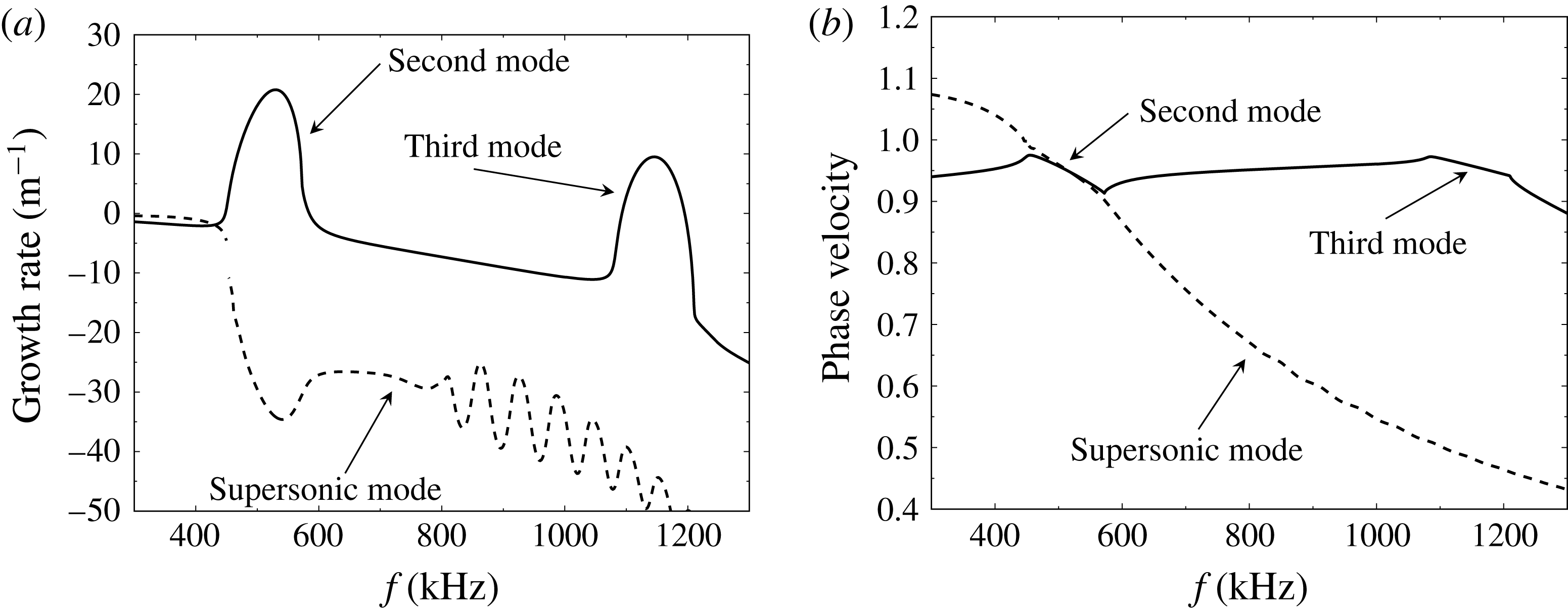
Boundary-layer modes at
 $s=1.70~\text{m}$
for case 2. The solid line represents the mode originating from the slow acoustic spectrum and the dashed line represents the mode originating from the fast acoustic spectrum.

It is shown here that as the nose radius increases, there is a downward shift of angular momentum in the boundary layer. There is also a shift towards the wall for the maximum temperature in the boundary layer. Accordingly, there is a shift in chemistry effects towards the wall and away from the boundary-layer edge. All of these shifts seem to suggest that the boundary layer is becoming more sensitive to wall effects, such as roughness. This was seen in the experiments of Stetson (Reference Stetson1983) where it was shown that roughness could move the transition location upstream for blunt cones.
4.2 LST analysis
Once the mean-flow simulations are complete, a theoretical analysis of the boundary-layer modes may be performed. Figure 4 shows the predicted growth rate and phase velocity for boundary-layer modes at the fixed location
 $s=1.70~\text{m}$
measured downstream along the surface starting from the cone nosetip. The dashed line corresponds to the mode that originates from the fast acoustic spectrum and the solid line corresponds to the mode that originates from the slow acoustic spectrum. This was originally shown by Fedorov & Khokhlov (Reference Fedorov and Khokhlov2001) for self-similar flow over a sharp cone but is also applicable to flow over a blunt cone.
Commonly, the most unstable boundary-layer mode for a slender vehicle in a near zero angle-of-attack flow is the second mode. Here, the second mode is contained in the frequency range 450–580 kHz where the growth rate is positive and the phase velocity ranges from 0.97 to 0.92. The growth rate of the second mode is large at this location and the second mode would likely be the physical mechanism to cause flow transition in the absence of bypass mechanisms such as effects due to surface roughness. This type of behaviour for the second mode has been well studied and is expected for relatively sharp geometries such as that found in case 2.
Boundary-layer modes at
 $s=2.00~\text{m}$
for case 3. The solid line represents the mode originating from the slow acoustic spectrum and the dashed line represents the mode originating from the fast acoustic spectrum.

For these flow conditions, the third mode is also unstable. It is contained in the frequency range 1080–1200 kHz where the phase velocity ranges from 0.97 to 0.95. The maximum growth rate is about half that of the second mode, so it will grow, but not as much as the second mode.
While often unnoticed, the supersonic mode is also present in the boundary layer of slightly blunted cones. For case 2, the supersonic mode is contained in the frequency range 600–1200 kHz. The growth rate over this range decreases from
 $-30$
to
 $-50~\text{m}^{-1}$
. Clearly, the supersonic mode is strongly damped and it would likely not lead to transition. For this reason, this mode is usually neglected as it is not a significant contributor to boundary-layer transition for sharp geometries.
Case 3 is set up in the same way as case 2 with the single difference being the nose radius for case 3 is increased to four times that of case 2. The growth rate and phase velocity of case 3 at
 $s=2.00~\text{m}$
is shown in figure 5. Here, the second mode is contained in the region of positive growth rate near 310–330 kHz. The growth rate of the second mode is small at this location and the frequency range over which it is unstable is narrow. The growth rate is small enough that with such a narrow frequency band it would be quite unlikely to lead to flow transition. Also note the frequency range over which the fast and slow modes are synchronized is greatly reduced (
 ${\sim}20~\text{kHz}$
) when compared to that of case 2 (
 ${\sim}130~\text{kHz}$
). It is possible that this plays a role in damping the second mode as the fast and slow acoustic modes have less time to resonate and exchange energy.
There is another larger region of positive growth rate in the frequency range 410–550 kHz that is not attributable to the second mode. One could easily question if the modal growth is due to the supersonic mode or the third mode. There are a couple of ways to distinguish the third mode from the supersonic mode. First, the phase velocity of the third mode is comparable to the second mode, which is
 $c_{r}\geqslant 1-1/M_{e}$
, so it should be above 0.9 for edge Mach numbers above ten. In contrast, Mack (Reference Mack1969) showed that the supersonic mode has a phase velocity
 $c_{r}<1-1/M_{e}$
which is less than the second mode. Second, Mack (Reference Mack1984) showed that the real part of the pressure eigenfunction crosses the zero axis twice for the third mode. For the supersonic mode, it has been shown that the real part of the pressure eigenfunction crosses the zero axis once inside the boundary layer and is oscillatory in the free stream, crossing the zero axis many more times. For both of these criteria, the modal growth in the frequency range 410–550 kHz has characteristics similar to the supersonic mode, not the third mode. The phase velocity is less than 0.9 and the real part of the pressure eigenfunction crosses the zero axis many times.
Although not easily recognizable, the third mode has been plotted in figure 5 also. It is in the frequency range 760–770 kHz. Its increase in growth rate is barely visible as it has been strongly damped by the increased nose radius of case 3. However, this is indeed the third mode as the phase velocity and eigenfunction are consistent with the third mode.
Downstream of
 $s=2.00~\text{m}$
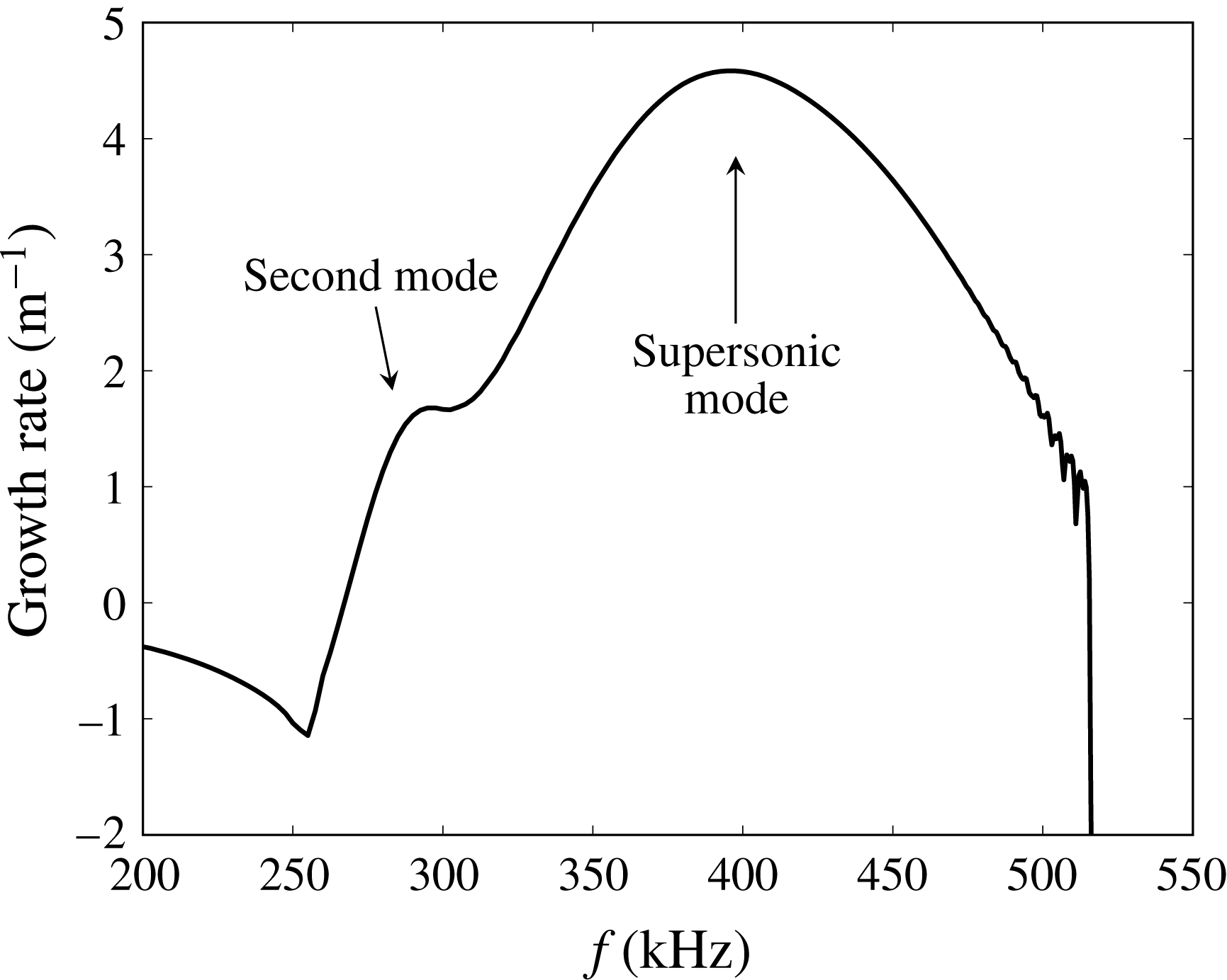
for case 3, the unstable regions for the second and supersonic modes grow closer and closer together. Eventually, they merge and form a large connected region of instability. Figure 6 shows the growth rate of the second and supersonic modes at
 $s=3.00~\text{m}$
for case 3. Both modes are unstable but now it is not clear where one ends and the other begins. The phase velocity and eigenfunctions show that the bump near 300 kHz is the second mode while higher frequencies are the supersonic mode. This large region of merged growth rate persists indefinitely downstream.
Growth rate of boundary-layer modes at
 $s=3.00~\text{m}$
for case 3.

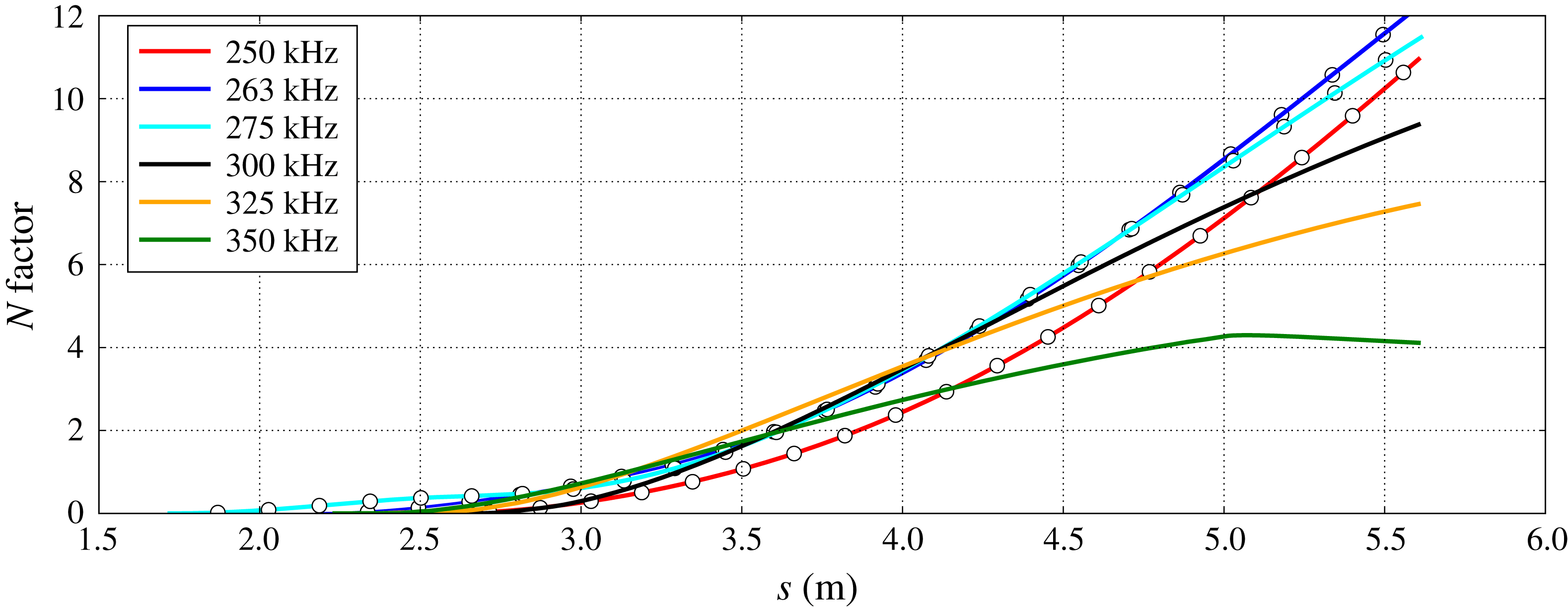
To estimate the transition location for cases 2 and 3, an
 $N$
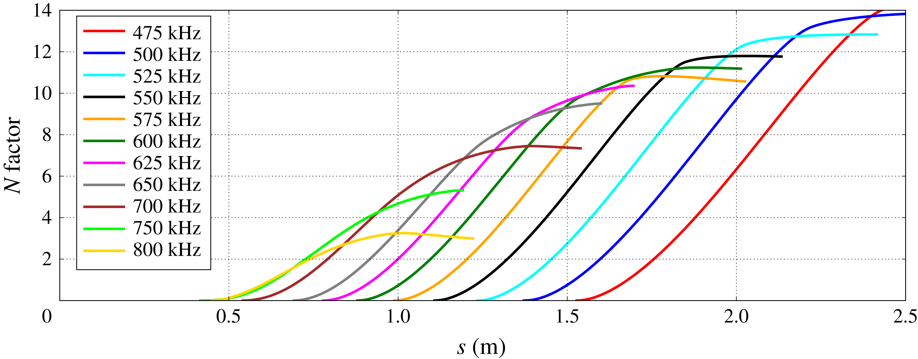
factor is computed along the surface of the cone. Figure 7 shows the
 $N$
factor plotted along the surface streamline for case 2. Each of the
 $N$
factors is from the integrated growth of the second mode. Using the criteria that free-flight
 $N$
factors are commonly near ten, transition onset is estimated to occur at
 $s=1.56~\text{m}$
and to be caused by the 600 kHz second-mode wave.
 $N$
factors for case 2 (
 $r_{n}=8.9~\text{mm}$
) from the second mode.

 $N$
factors for case 3 (
 $r_{n}=35.6~\text{mm}$
) from the supersonic mode (——) and the second mode (–
 $\circ$
–).

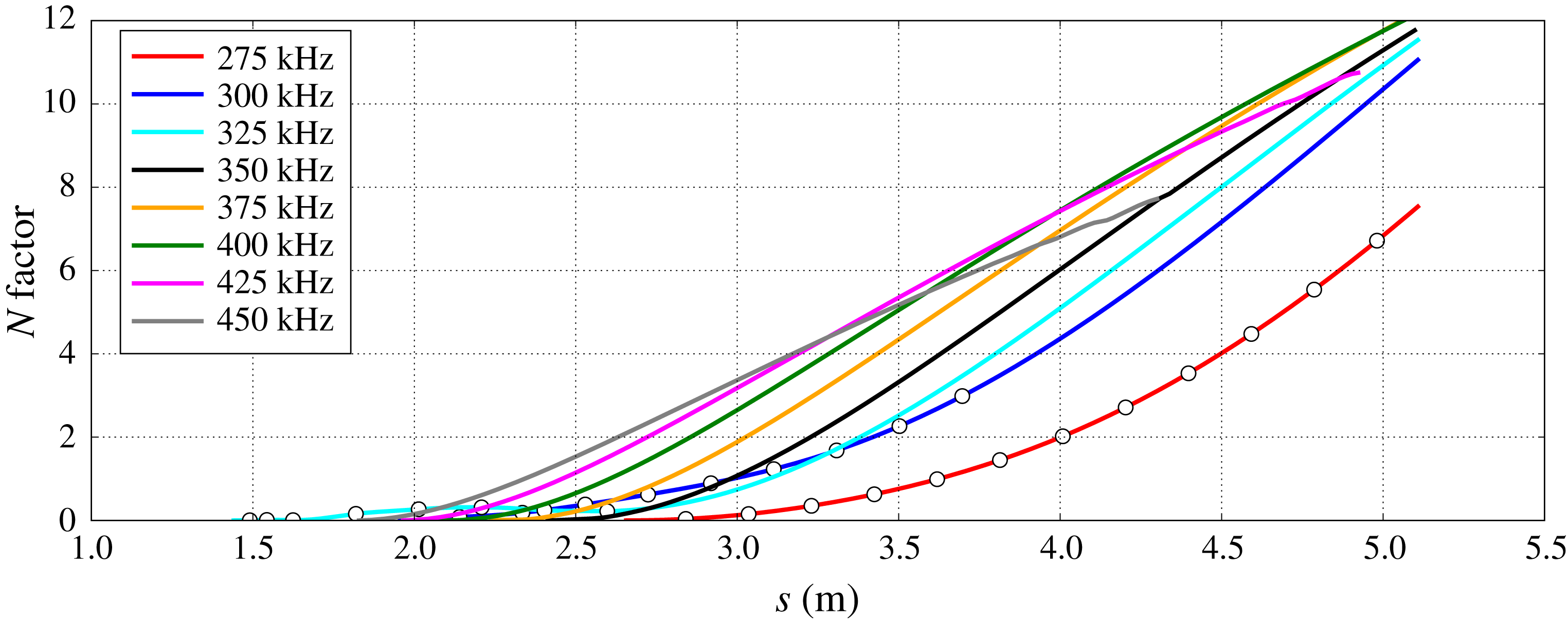
Figure 8 shows the
 $N$
factor plotted along the surface streamline for case 3. For case 3,
 $N$
factors are computed from the second mode (–
 $\circ$
–) and the supersonic mode (——). Note that for the frequencies where the second mode transitions to the supersonic mode, there is not an immediate switch from one mode to the other. Rather, the phase velocity of the supersonic mode gradually decreases and the eigenfunction of the second mode slowly changes until it matches that of the supersonic mode. Mack (Reference Mack1987) also showed that the second mode was attached to the supersonic mode for cold wall flows.
Using an
 $N$
factor of ten, transition onset is estimated to occur at
 $s=4.57~\text{m}$
and to be caused by the 400 kHz supersonic-mode wave. Notice that the
 $N$
factor of the second mode trails that of the supersonic mode for case 3. In other words, for a fixed
 $N$
factor, the second mode reaches the value of the
 $N$
factor downstream of the supersonic mode. A transition estimate using only the second mode is
 $s=5.40~\text{m}$
at a frequency of 275 kHz. This is a difference of 0.8 m. A transition estimate that does not take into account the supersonic mode would estimate transition to be approximately 0.8 m downstream of an estimate using the supersonic mode for case 3.
When comparing cases 2 and 3, the most intriguing aspect is the change of which boundary-layer mode is the most unstable. For case 2, the second mode is clearly the most unstable boundary-layer mode. As a matter of fact, the supersonic mode is nowhere near unstable. However, as the nose radius is increased in case 3, not only does the supersonic mode become unstable, it surpasses the second mode as the most unstable boundary-layer mode. In the absence of bypass transition, it would seem that for case 2 the second mode would lead to transition, while for case 3 the supersonic mode would lead to transition.
4.2.1 Effects of increased nose radius on the supersonic mode
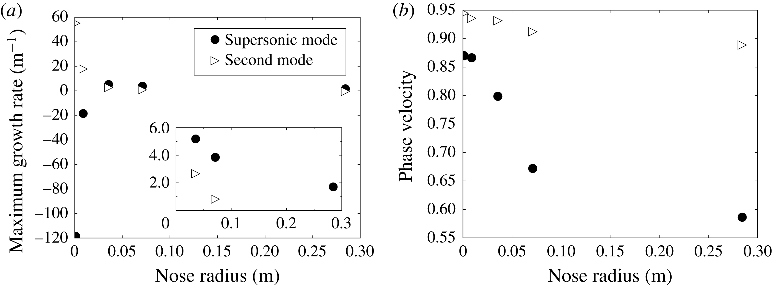
As an initial increase in nose radius made the supersonic mode unstable, a logical next step would be to determine if the growth rate of the supersonic mode continued to increase with increasing nose radius. Figure 9(a) shows the growth rate of the second and supersonic modes when the
 $N$
factor of each separate case is 5. The streamwise locations for comparison are 0.25 m, 1.00 m, 3.42 m, 4.87 m and 8.12 m for cases 1–5, respectively. This is a somewhat arbitrary choice for comparison between cases with varying nose radius and is meant to show the trend for each mode’s growth rate slightly upstream of transition.
Comparison between the second and supersonic modes of (a) the maximum growth rate and (b) the phase velocity at that frequency at the streamwise location where
 $N=5$
.

For a sharp nose, i.e. zero nose radius, figure 9(a) shows a very stable supersonic mode. For
 $r_{n}=36~\text{mm}$
, the supersonic mode has become unstable and is slightly more unstable than the second mode. In other words, as the cone is blunted from the initially sharp case, the supersonic mode moves from very stable to more unstable than the second mode. This is behaviour that has not previously been reported in the open literature. Also, it is quite clear why the supersonic mode has garnered little attention as many studies of hypersonic boundary-layer transition have focused on sharp, or near sharp, geometries. As the nose radius is further increased beyond 0.036 m, the trend changes and the growth rate of the supersonic mode begins to gradually decrease with increasing nose radius. Note that figure 9(a) shows the growth rate at one specific location which does not show by itself which mechanism would lead to transition. However, for this specific case, blunting the cone has a strong destabilizing effect on the supersonic mode.
Comparison of growth rate for the second (
 $f\approx 325~\text{kHz}$
) and supersonic (
 $f\approx 475~\text{kHz}$
) modes for case 3 at
 $s=2.00~\text{m}$
. The heat of formation for atomic oxygen is either positive or negative.

It is likely that the growth rate of the supersonic mode is influenced by chemical reactions as originally shown by Chang et al. (Reference Chang, Vinh and Malik1997). They found that the growth of the supersonic mode seemed to depend strongly on how chemical reactions were modelled. For a Mach 20 flow over a six degree sharp wedge, they showed that an assumption of chemical equilibrium created a more unstable supersonic mode than using finite-rate chemical reactions. Also, the supersonic mode was not unstable when chemical reactions were neglected, i.e. a perfect-gas assumption was used.
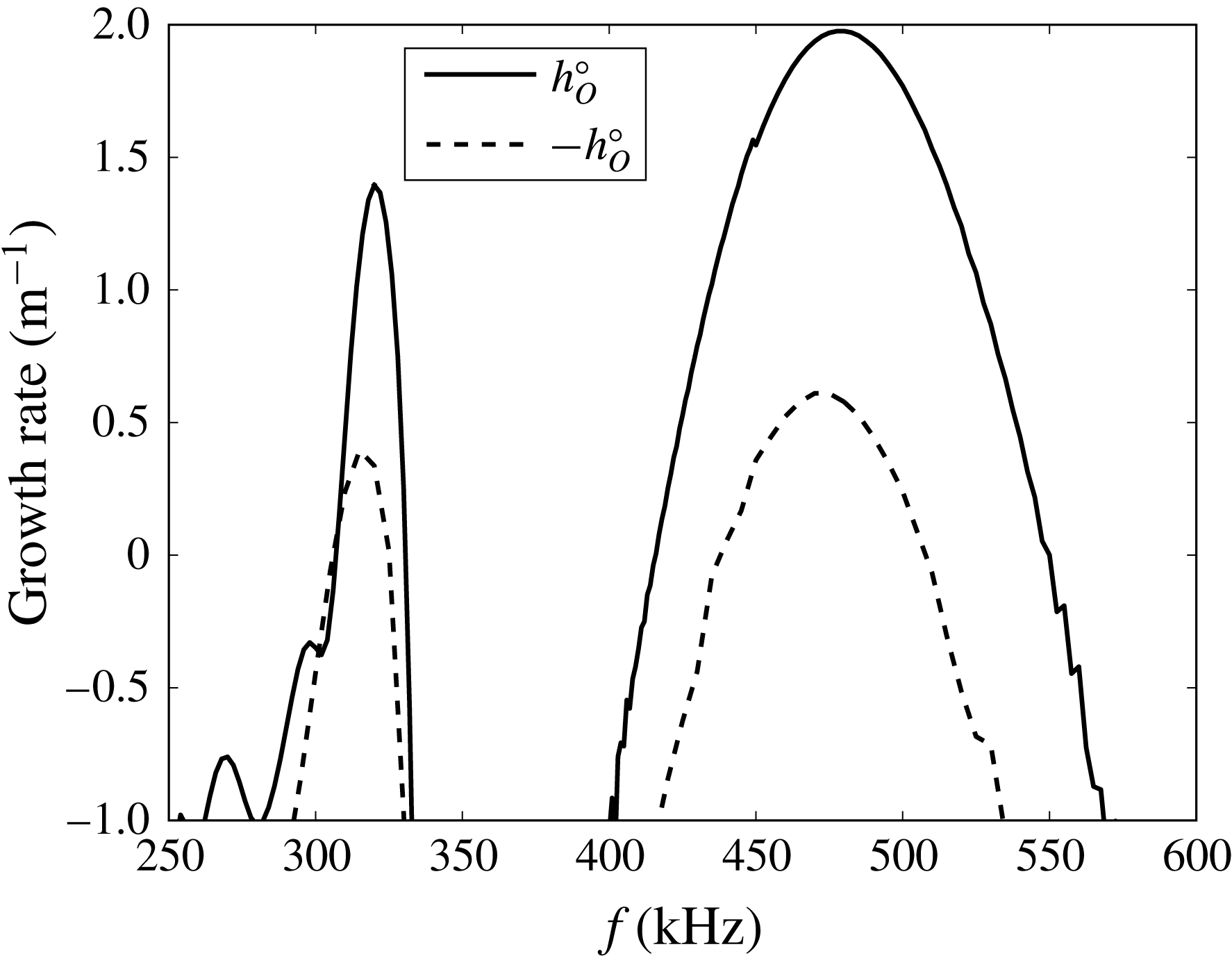
Figure 10 shows the growth rate of the second and supersonic modes at
 $s=2.00~\text{m}$
for case 3 when the heat of formation is modified in the instability wave only. The solid line corresponds to the unchanged heat of formation for atomic oxygen, while the dashed line corresponds to a sign change of the heat of formation for atomic oxygen. At this location in the boundary layer, the main chemical reaction is the recombination of atomic oxygen which adds heat to the flow. Note that when the sign is changed for
 $h_{O}^{o}$
, a decrease in the growth rate shows that recombination of atomic oxygen is destabilizing. Conversely, an increase in the growth rate would show that recombination of atomic oxygen is stabilizing. For both the second and the supersonic modes, recombination of atomic oxygen is destabilizing. However, for the supersonic mode, this destabilizing effect is more pronounced than for the second mode. One reason for this is the supersonic mode depends more on near wall properties and that is where there is more recombination of atomic oxygen. Note that the direction of the chemical reaction is important. It is the recombination of atomic oxygen that destabilizes the modes while the dissociation of oxygen would stabilize the modes.
Recall figure 3(d) which showed the amount of atomic oxygen in the boundary layer for each case. For
 $r\leqslant 0.05~\text{m}$
, there is an increase in atomic oxygen and an increase in the growth rate of the supersonic mode. For
 $r\geqslant 0.05$
, chemical reactions continue to increase but there is a decrease in the growth rate of the supersonic mode. It appears that while recombination of atomic oxygen may initially increase the growth rate of the supersonic mode, there must be other factors that lead to its decay at large nose radii.
The technique of modifying the chemical properties of the instability wave has been used previously by Johnson, Seipp & Candler (Reference Johnson, Seipp and Candler1998) to study the effects of chemical reactions on second-mode waves. They found that, depending on whether the reaction was endothermic or exothermic, a second mode wave could be stabilized or destabilized by the reaction. This statement is similar to stating that the direction of the reaction determines whether a reaction is stabilizing or destabilizing, as heat is absorbed or released, depending on which direction the reaction takes. Recombination of atomic oxygen is exothermic and is shown here to destabilize supersonic-mode waves. This is the same conclusion Johnson et al. (Reference Johnson, Seipp and Candler1998) arrived at for second-mode waves. Note however, that this applies to the effects in the instability wave and is separate from any effects the reaction may have on changing the mean flow.
Also shown in figure 9(a) is the growth rate of the second mode. There is a marked decrease in growth rate for the second mode as the nose radius increases. This decrease in growth rate of the second mode with increasing nose radius is consistent with an abundant amount of previous research where two notable examples are Malik et al. (Reference Malik, Spall and Chang1990) and Lei & Zhong (Reference Lei and Zhong2012).
Similar to the plot of growth rate for varying nose radii, the phase velocity of the second and supersonic modes at
 $N=5$
is plotted in figure 9(b). As the nose radius increases, the flow velocity behind the shock decreases which leads to a decrease in the phase velocity of the second mode. Similarly, the phase velocity of the supersonic mode decreases as the nose radius increases. Also, the difference between the phase velocity of the supersonic mode and the second mode increases as the nose radius increases.
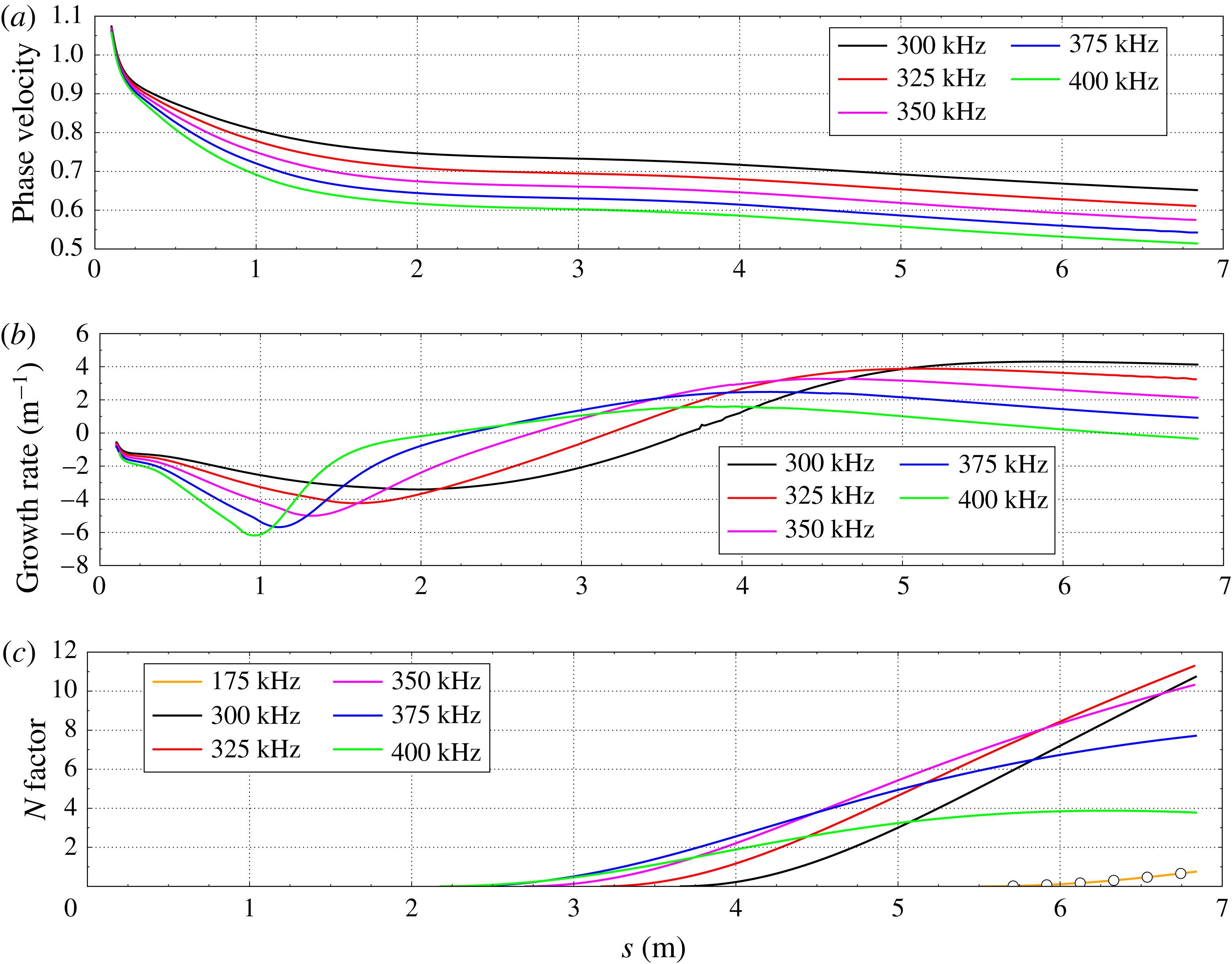
Cases 4 and 5 are the largest nose radius cases tested here. Unlike case 3, there is no merging of the second and supersonic modes. Also, the supersonic mode is clearly the most unstable mode for both cases. Figure 11 shows the phase velocity, growth rate and
 $N$
factor of the supersonic mode along the length of the cone for case 4. For this case, the fast acoustic mode separates from the fast acoustic spectrum near the blunt nose. The phase velocity of the fast acoustic mode begins to decrease and moves towards the phase velocity of the slow acoustic mode. Notice that there is no clearly defined synchronization region here. As the phase velocity continues to decrease, the fast acoustic mode transitions to the supersonic mode. It is interesting to note that the phase velocity of the supersonic mode increases with decreasing frequency.
Supersonic modes for case 4. (c)
 $N$
factors from the supersonic mode (——) and the second mode (–
 $\circ$
–).

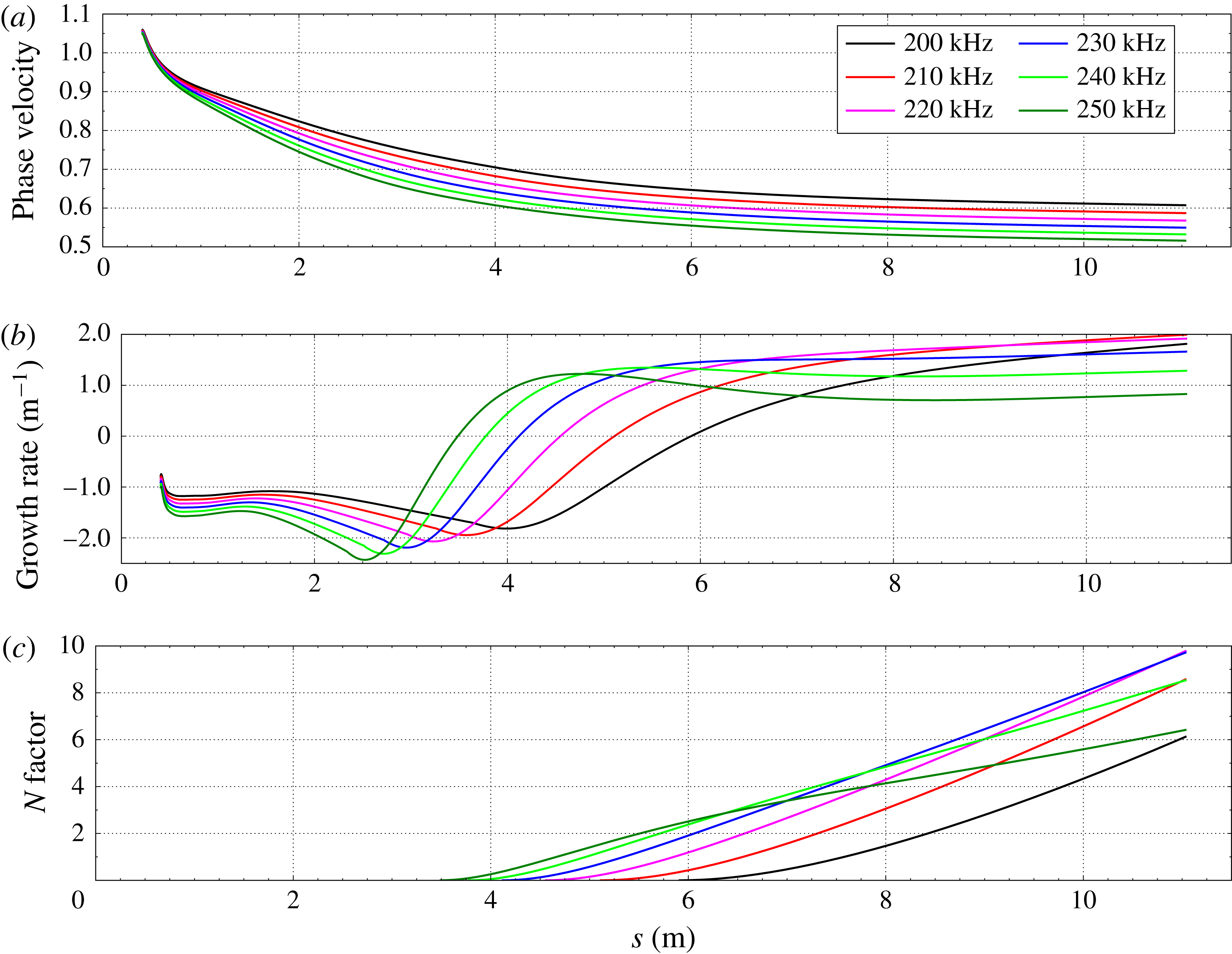
Supersonic modes for case 5. (c)
 $N$
factors from the supersonic mode.

The growth rate of the supersonic mode shows a dip in growth rate as the fast acoustic mode transitions to the supersonic mode. The supersonic mode becomes unstable near
 $s=2.00~\text{m}$
and reaches a maximum growth rate of
 $4.4~\text{m}^{-1}$
. Note that wiggles in the growth rate of the supersonic mode can occur if the eigenfunction in the inviscid region is not properly resolved in the LST solver.
The
 $N$
factor for case 4 is shown in figure 11(c) for the supersonic mode (——) and the second mode (–
 $\circ$
–). The main conclusion from this plot is the relative insignificance of the second-mode
 $N$
factors compared to the
 $N$
factors of the supersonic mode. The 325 kHz supersonic mode reaches an
 $N$
factor of ten at 6.44 m. At the same location, the largest
 $N$
factor from the second mode is 0.4 which is due to the 175 kHz second mode. One reason for this difference is the locations where instability starts for each mode. The second mode first becomes unstable near 4.5 m while the supersonic mode becomes unstable near 2.0 m. This is a large difference which is in contrast to case 3 (recall figure 8). In case 3, the second mode and the supersonic mode instabilities begin at similar streamwise locations.
The phase velocity, growth rate and
 $N$
factor of the most unstable supersonic modes for case 5 are shown in figure 12. Case 5 is the largest nose radius case simulated here and is two times that of case 4. The phase velocities of the supersonic mode are similar to those of case 4. Each start from the fast acoustic spectrum and the highest frequency supersonic mode has the lowest phase velocity. The growth rates show a similar pattern to those of case 4 as well. The highest growth rate at
 $N=10$
has been cut in half from near four per metre to two per metre.
A notable difference between cases 4 and 5 is in the
 $N$
factor plot of figure 12(c). For both cases, the supersonic mode will likely lead to transition before the second mode. However, for case 5, the second mode is not unstable at
 $s=11.0~\text{m}$
when the
 $N$
factor from the supersonic mode is ten. For case 4, the second mode is unstable when
 $N=10$
but the growth rate is small. As the nose radius increases for these flow conditions, the difference in the location of instability onset between the supersonic and second modes increases. In other words, the location of instability onset is moved downstream for each mode, but the second-mode location of instability onset is moved further downstream.
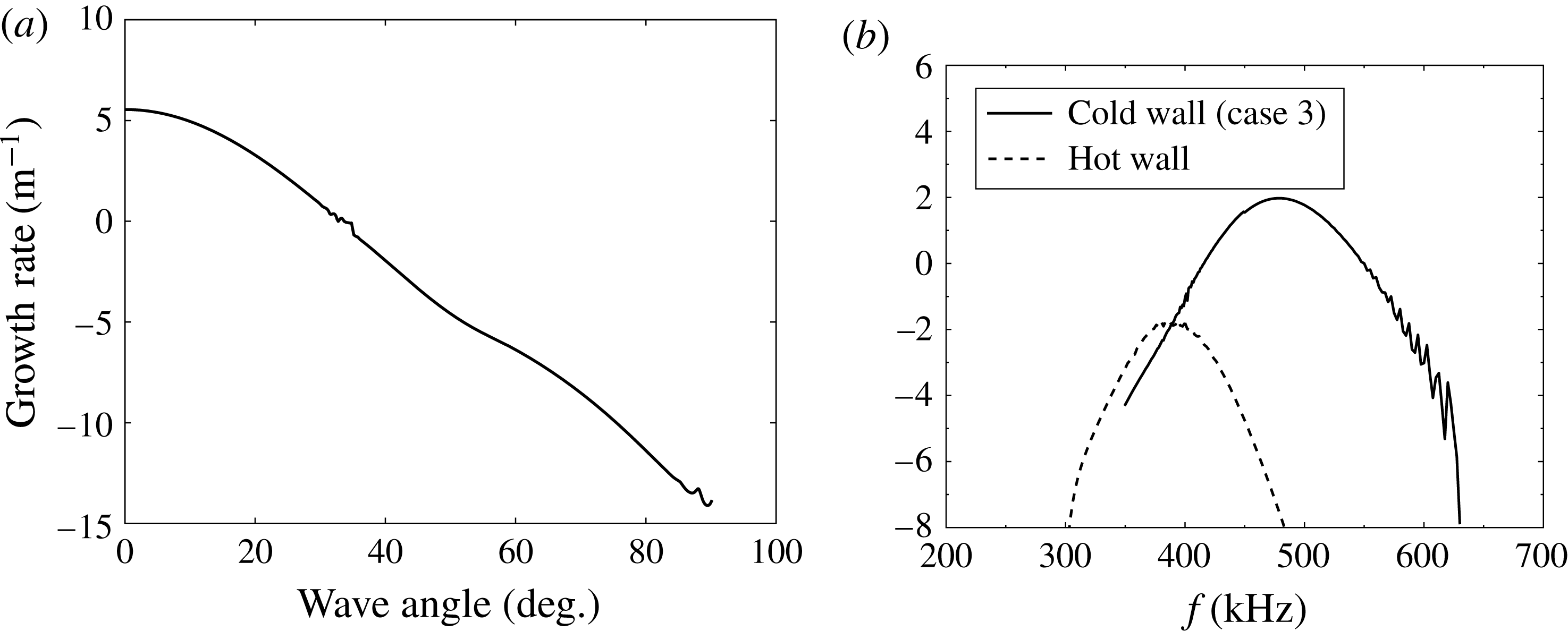
(a) Growth rate of 350 kHz supersonic mode with varying wave angle for case 3 at
 $s=4.00~\text{m}$
. (b) Comparison of growth rate for hot and cold wall cases at
 $s=2.00~\text{m}$
.

It should be noted that, for large nose bluntness, transition is reversed and moves upstream. This is termed transition reversal and was shown experimentally in the ground tests of Stetson & Rushton (Reference Stetson and Rushton1967). The exact physical mechanisms that cause transition reversal in blunt cones are still not well understood. For the cases computed here, for which the supersonic mode becomes dominant, the nose radii may be large enough that the physical mechanisms that cause transition reversal would be present. In other words, it is possible that the nose radii may be large enough that the transition reversal mechanisms would have taken over and the supersonic mode would not cause transition. However, identifying the nose radius where transition reversal would occur for the conditions simulated here is beyond the scope of this paper.
4.2.2 Parametric effects on supersonic modes
In Mack (Reference Mack1984) it was shown that the second mode is the most unstable when its phase velocity is aligned with the flow velocity. This holds for flat plates as well as cones. This information is quite useful from a DNS standpoint. It means that when simulating a second-mode wave in an axisymmetric flow, high grid resolution is only needed in the streamwise and wall-normal directions and is not needed in the transverse direction. This reduces the computational cost significantly. Figure 13(a) shows the variation of the spatial growth rate with wave angle for a 350 kHz supersonic mode for case 3 at
 $s=4.00~\text{m}$
. It should be noted that there are only a finite number of wave angles that yield a consistent solution for a cone, but the wave angle has been plotted as if it were continuous. A wave angle of zero corresponds to an alignment of the phase velocity of the supersonic mode with the flow velocity. As the wave angle increases from zero, there is a velocity component of the wave in the transverse direction. Fortunately, the growth rate is a maximum at a wave angle of zero which is similar to the growth rate of the second mode. This greatly reduces the computational cost of a DNS. Only a two-dimensional axisymmetric DNS is required to simulate the most unstable supersonic mode for a cone at zero degree angle-of-attack for these specific flow conditions.
In Mack (Reference Mack1987) it was shown for a Mach 5.8 flow over a flat plate that the supersonic mode was unstable when
 $T_{w}/T_{r}<0.25$
. This could also be stated as an increase in the wall-temperature stabilized supersonic-mode waves. To bound the effect of wall heating on the supersonic mode for a blunted cone, a mean-flow simulation is run where the wall boundary condition for temperature is maintained as a radiative wall condition throughout the cone frustum. Recall that for cases 2–5 the wall temperature, which is shown in figure 2, is exponentially lowered to 460 K on the cone frustum. The boundary condition
 $\hat{T}_{wall}=0$
in the LST code is the same for both hot and cold wall cases. Figure 13(b) shows a comparison of the growth rate for the supersonic mode between the hot and cold (case 3) wall cases at
 $s=2.00~\text{m}$
. At this location, the wall temperature of the hot wall is 1867 K and the ratio to the stagnation temperature is 0.10. The supersonic mode is damped when the wall is heated. This damping decreases downstream. Along with the damping effect, there is a frequency shift for the hot wall case to lower frequencies. This frequency shift coincides with a thickening of the boundary layer due to an increase in wall temperature.
 $N$
factors for case 3 (
 $r_{n}=35.6~\text{mm}$
) with a hot wall from the supersonic mode (——) and the second mode (–
 $\circ$
–).

 $N$
factors for case 3 with a hot wall are shown in figure 14 for the supersonic mode (——) and the second mode (–
 $\circ$
–). Note that for both modes, an increase in wall temperature has been stabilizing. However, the supersonic mode has been damped more than the second mode. For the cold wall case, the supersonic mode reached an
 $N$
factor of ten before the second mode. For the hot wall case, the second mode reaches an
 $N$
factor of ten before the supersonic mode. A switch of the most unstable mode from the supersonic mode to the second mode occurs for case 3 (
 $r_{n}=35.6~\text{mm}$
) when the wall-temperature ratio is changed from
 $T_{w}/T_{o}=0.026$
to
 $T_{w}/T_{o}=0.10$
. One factor for the increased damping of the supersonic mode is that an increase in wall temperature will slow the recombination of atomic oxygen. Recall figure 10 where it was shown that recombination of atomic oxygen has a stronger effect on the supersonic mode than the second mode.
4.3 Supersonic modes in ground test experiments of blunted cones
There have been many ground tests of blunted cones in hypersonic flows which show transition delay. For these experiments, is there likely to be significant growth of the supersonic mode as the nose radius increases? To answer this question, a set of free-stream conditions from Softley (Reference Softley1968) were simulated for varying nose radii. The free-stream conditions are
 $M=9.5$
,
 $T=76.7~\text{K}$
,
 $p=319~\text{N}~\text{m}^{-2}$
,
 $c_{N_{2}}=0.78$
and
 $c_{O_{2}}=0.22$
. The free-stream stagnation enthalpy is
 $1.48~\text{MJ}~\text{kg}^{-1}$
and the unit Reynolds number is
 $4.60\times 10^{6}~\text{m}^{-1}$
. The wall temperature of the cone is assumed to be at room temperature (
 $T_{w}/T_{o}=0.21$
). The free-stream stagnation enthalpy and wall-temperature ratio are similar to other ground test conditions showing transition delay for large nose bluntness.
Three separate cases were simulated with nose radii of 1.27 mm, 12.7 mm and 25.4 mm. The first two cases spanned the region of transition delay for the blunted cone. The third case was well into the transition reversal region for large nose bluntness. For each of these cases, there was no significant supersonic-mode growth. In other words, the supersonic mode is not unstable for any of the tested nose radii with these free-stream conditions.
There are a few differences between the free-stream conditions for the simulated ground tests and those of cases 1–5, i.e. the reentry conditions, that could account for the lack of supersonic-mode growth. The first difference is the higher
 $T_{w}/T_{o}$
in the ground test conditions. Recall from figure 14 that changing the wall-temperature ratio from 0.026 to 0.10 caused a switch in the instability mode that lead to transition from supersonic to second. For the ground test conditions,
 $T_{w}/T_{o}=0.21$
which is even larger than the hot wall conditions of case 3. Therefore, this strong effect of wall-temperature ratio on the supersonic mode may make it unlikely to see significant growth of the supersonic mode for the simulated ground tests.
Another difference between the free-stream conditions is the stagnation enthalpy. The free-stream stagnation enthalpy of the reentry conditions is an order of magnitude greater than that of the ground test conditions. As the stagnation enthalpy increases, there is an increase in the amount of chemical reaction in the flow. The amount of chemical reaction in the ground tests is nearly zero. In fact, the flow would be best modelled by a perfect gas. However, as shown in figure 3, there is a significant amount of chemical reaction occurring in the flow around a blunted cone at reentry conditions. The main pathway for chemical reaction, recombination of atomic oxygen, destabilizes the supersonic mode more than the second mode for a blunted cone. It is possible that a low stagnation enthalpy, which leads to a lack of oxygen recombination in the boundary layer, stabilizes the supersonic mode in the ground tests.
A third difference between the free-stream conditions is the Mach number. The reentry conditions simulated here have a much higher Mach number than the simulated ground test conditions. It is possible that there is also some effect of Mach number on increasing the instability of the supersonic mode. Further work would be needed to evaluate and understand this effect.
4.4 DNS of supersonic mode
To further understand the supersonic modes, a DNS is run. It is run to find if DNS also shows the existence of supersonic modes and if the properties of the modes are consistent between the two markedly distinct methods of LST and DNS. The DNS results shown here are for a single frequency disturbance that is imposed at the inlet (recall figure 1) using the eigenfunction from LST with an arbitrary amplitude. The amplitude of the disturbance needs to be large enough that the simulation is not contaminated by numerical errors, i.e. the prescribed amplitude is larger than the tolerance to which the mean flow is converged, but small enough that the disturbance is still linear. Also, the imposed disturbance is only an oscillating eigenfunction imposed at one location. The growth, or decay, of the imposed disturbance is dependent on the DNS and is not specified at the inlet.
Instantaneous perturbation of translation–rotation temperature.

The DNS grid has 640 grid points in the wall-normal direction between the body and the shock. Of these points, 250 are inside the boundary layer. The grid spacing in the streamwise direction is
 $9\times 10^{-4}~\text{m}$
. This resolves the streamwise wavenumber of the 350 kHz supersonic mode which is near
 $71~\text{m}^{-1}$
over the domain simulated. The total streamwise domain of the DNS is
 $4.0~\text{m}<s<4.7~\text{m}$
. Grid resolution was checked by running a domain of smaller streamwise extent with 1280 wall-normal points.
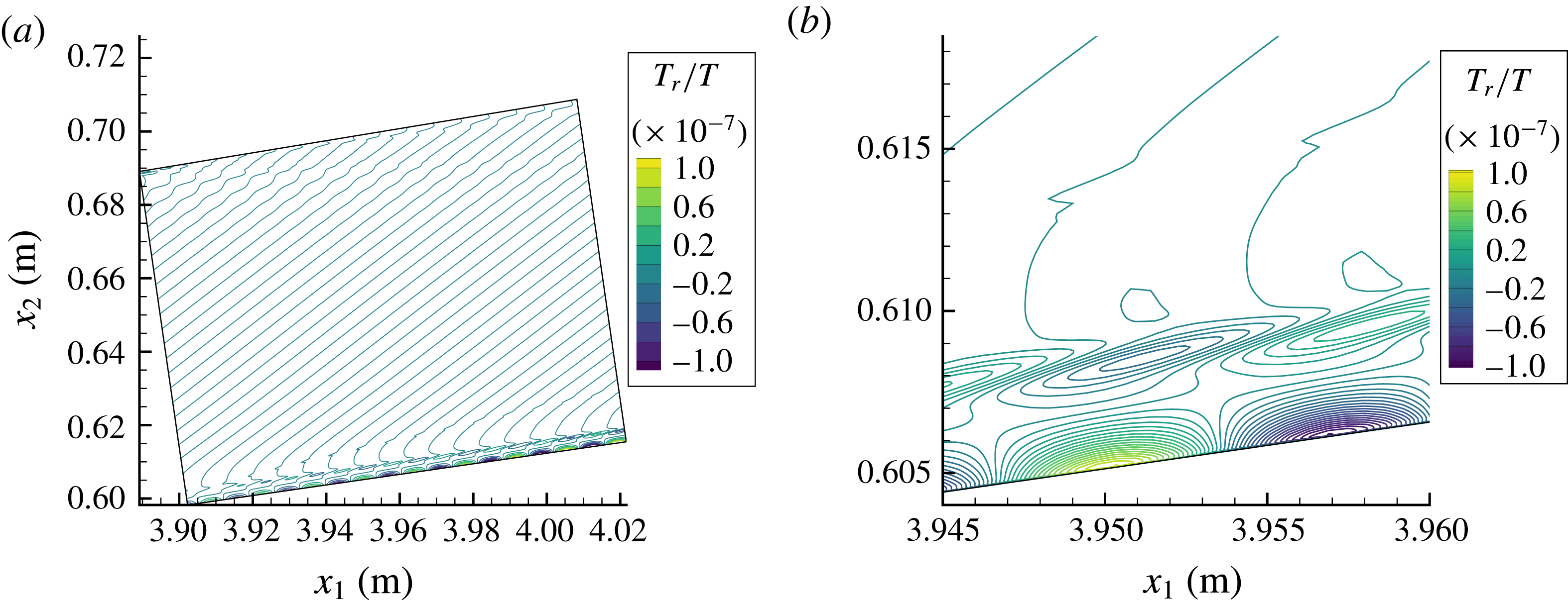
Figure 15 shows two instantaneous snapshots of the perturbation of the translation–rotation temperature for the 350 kHz supersonic mode. The conditions are from case 3. The bottom of the simulated domain is the cone surface and the top is the shock wave. The flow is moving from left to right. The line normal to the body that bounds the domain on the left is the DNS inlet where the instability wave is imposed. When viewed along the cone’s axis, the inlet is an annulus whose inner radius is the body radius at
 $s=4.00~\text{m}$
and outer radius is the shock. Note the contour lines running across the domain outside of the boundary layer in figure 15(a). They are due to the oscillations in the eigenfunction of the supersonic mode outside of the boundary layer. These oscillations do not damp, rather they grow at a rate similar to the disturbance inside the boundary layer. However, they are generally an order of magnitude less than the disturbance near the wall.
In figure 15(b), a close up of the disturbance structure in the boundary layer is shown. The maximum amplitude for the temperature disturbance is near the wall. There is another local maximum near the edge of the boundary layer. For the second mode, this behaviour is reversed and the maximum amplitude is near the boundary-layer edge. This change in the maximum amplitude in the temperature eigenfunction between supersonic and second modes is consistent with the results of Chang et al. (Reference Chang, Vinh and Malik1997).
There is a sharp peak outside of the boundary layer near
 $y=0.615~\text{m}$
. This peak is a Mach wave that forms as the flow adjusts to the imposed perturbation at the inlet. The Mach wave continues downstream until eventually it will interact with the shock. It acts as a demarcation separating the region above the Mach wave from the region below. Any disturbance between the shock and the Mach wave is due to convection of the initial perturbation imposed at the inlet. While any disturbance below the Mach wave is not simply a disturbance convecting downstream, it is the directly simulated supersonic mode made without the simplifying assumptions used in LST.
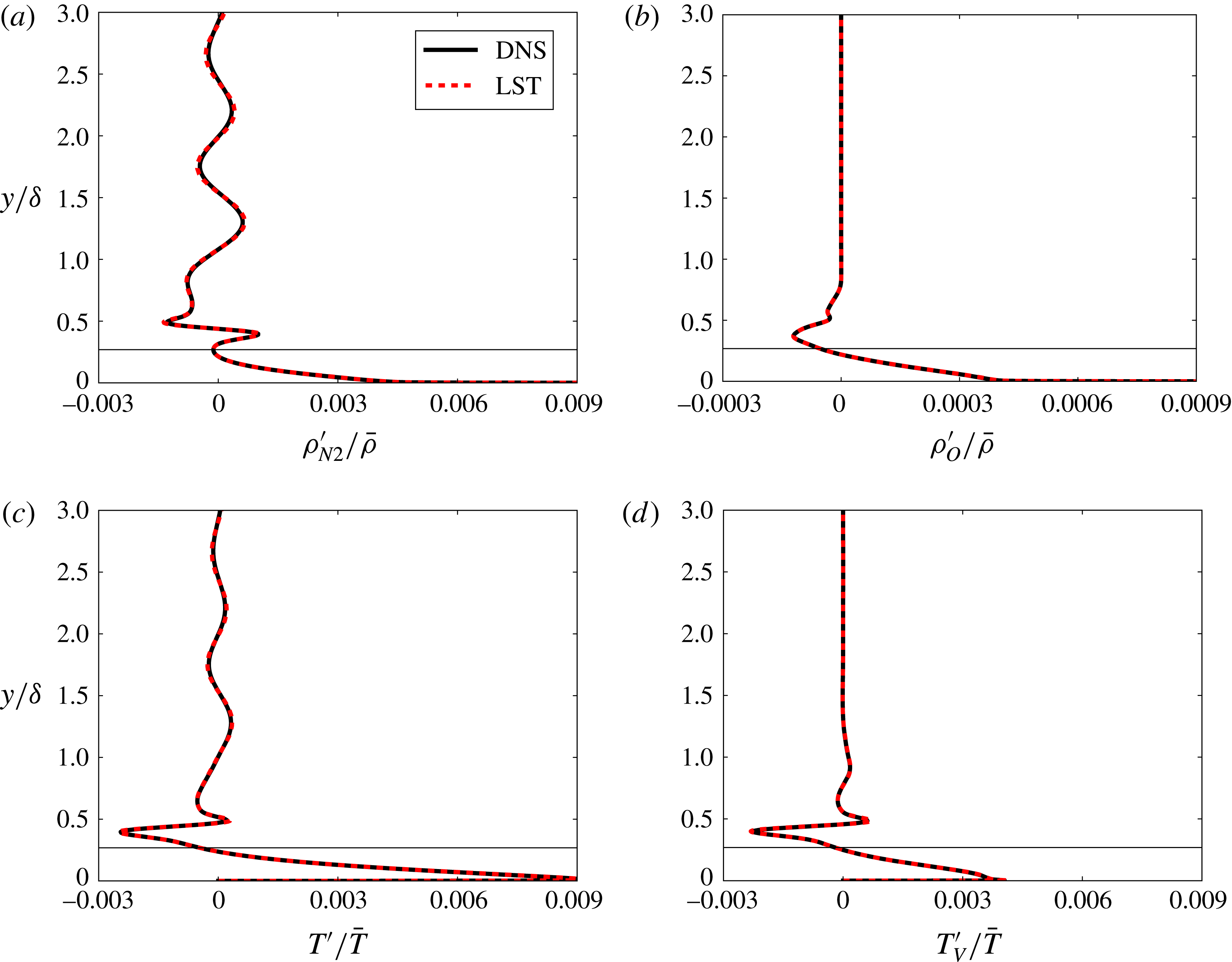
Comparison of instantaneous flow perturbations between DNS and LST for the 350 kHz supersonic mode. The wall-normal location of the sonic line is marked on each panel.

If a single wall-normal slice of the instantaneous DNS is taken, it may be compared to the real part of the eigenfunction from LST. A comparison of the instantaneous flow between DNS and LST is given in figure 16 for a 350 kHz supersonic mode at
 $s=4.66~\text{m}$
for case 3. The sonic line is marked in each of the plots. It is the wall-normal location
 $y_{s}$
where the flow velocity is equal to the phase velocity minus the local speed of sound
 $u(y_{s})=c_{r}-a(y_{s})$
. Near the wall and below the sonic line, there is adequate agreement between the two methods. Above the sonic line, the two methods are also in adequate agreement.
In figure 16(a), the amplitude of the oscillations outside the boundary layer are the same between the two methods, but they are slightly out of phase. There are no oscillations outside of the boundary layer for the density perturbation of atomic oxygen and vibration temperature. This is because the density of atomic oxygen is greatly reduced outside of the boundary layer. Also, the vibration temperature is nearly constant from the edge of the boundary layer to the shock. Chang et al. (Reference Chang, Vinh and Malik1997) noted that there were no oscillations of the eigenfunction in the free stream for any species. This is due to the fact that they plotted the perturbation of mass fraction for each species and a perturbation of density for each species is plotted here. In other words, the mass fraction of each species in the free stream does not vary, but the density of each species does vary.
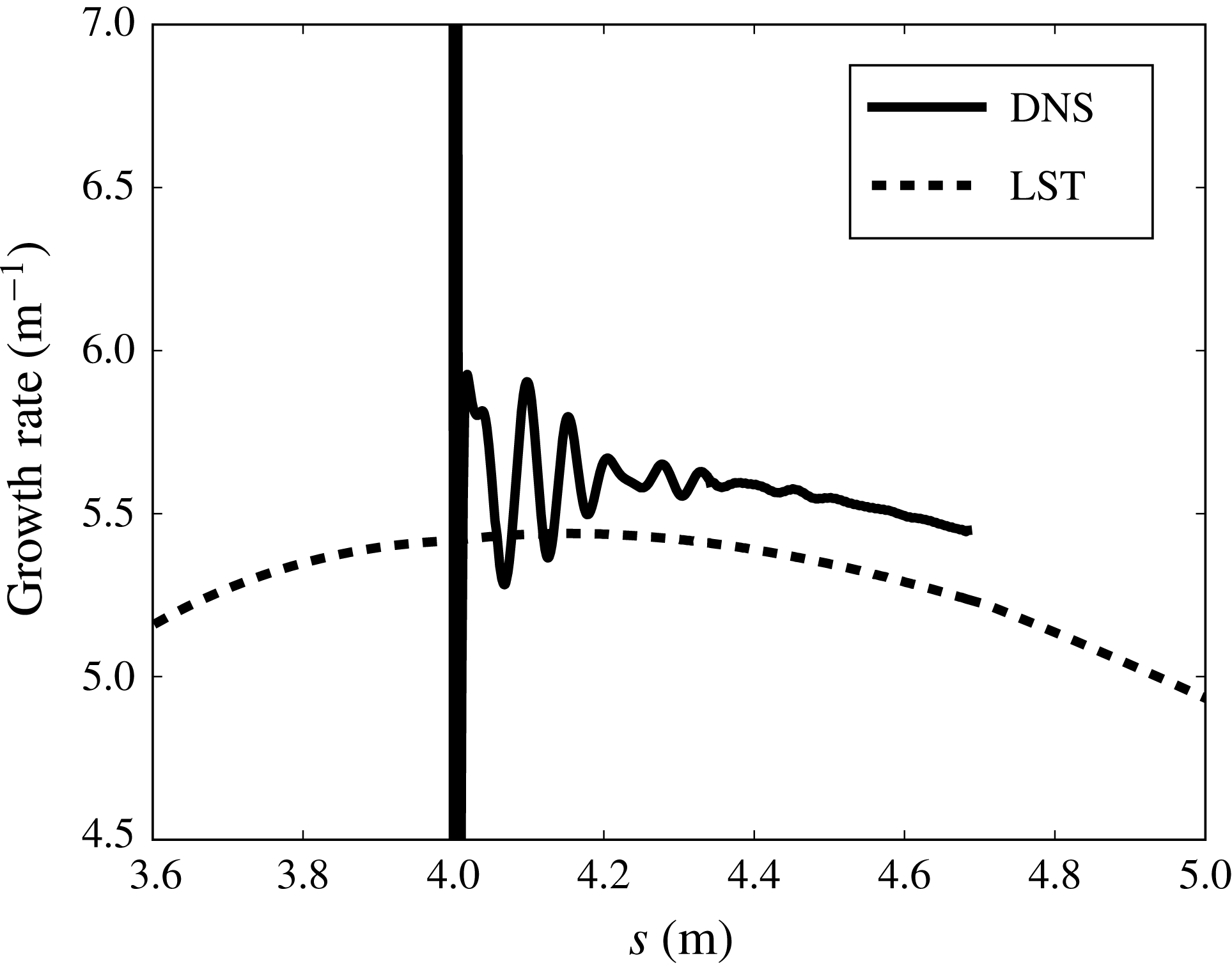
Comparison between DNS and LST for the growth rate of the supersonic mode at 350 kHz for case 3.

For each of figures 16(a)–16(d), note that the maximum amplitude for the eigenfunctions is at, or near, the wall. In fact, for all the perturbed variables, there is a significant decrease in the amplitude of the eigenfunction near the boundary-layer edge and an increase near the wall when compared to the second mode. With a larger amplitude near the wall, it would seem that the supersonic mode may be especially sensitive to surface roughness. This is a significant change as surface roughness is thought to play a strong role in boundary-layer transition for blunt cones (Schneider Reference Schneider2004). However, the supersonic mode appears at large distances downstream of the nose, while the sensitivity to roughness found in blunt cone experiments is near the nose. Also, recent promising numerical and experimental results have shown that the second mode can be stabilized in a hypersonic boundary layer when finite-height roughness are judiciously placed in the boundary layer (Fong et al. Reference Fong, Wang, Huang, Zhong, McKiernan, Fisher and Schneider2015; Mortensen & Zhong Reference Mortensen and Zhong2015). Would these results still hold for the supersonic mode? It would be quite instructive to learn how surface roughness affected the supersonic mode.
The phase velocity of the supersonic mode found using LST compares well with DNS. The per cent error is less than 0.25 % over the length of the simulated domain for multiple frequencies of the supersonic mode. Figure 17 shows a comparison of the growth rate between DNS and LST for a 350 kHz supersonic mode. The comparison begins at
 $s=4.0~\text{m}$
as that is where the instability wave is initially imposed in the DNS. The DNS growth rate is determined from the increase in the wall-pressure perturbation. The trend of slightly decreasing growth rate is the same for both methods, but the growth rate from DNS is consistently around
 $0.20~\text{m}^{-1}$
or 4 % higher than the growth rate from LST. Likely it is non-parallel effects that make the growth rate higher in the DNS. Commonly, non-parallel methods such as PSE have
 $N$
factors at transition that are larger than LST (Chang et al.
Reference Chang, Vinh and Malik1997; Malik Reference Malik2003). This means that growth rates predicted from PSE are generally larger than those from LST. A slightly higher growth rate for the directly simulated supersonic mode is consistent for case 3 when the frequency of the supersonic modes is changed.
An interesting aspect that arises when comparing the growth rate between DNS and LST is the choice of where to compare the growth rate and what variable in the DNS to use to compute the growth rate. A suggestion could be made that perhaps the growth rate will compare better between the two methods if it is compared near the generalized inflection point, or if a different variable is used to compute the growth rate. Figure 18 shows the growth rate at
 $s=4.66~\text{m}$
computed from DNS results using three separate flow variables (
 $p^{\prime }$
,
 $u^{\prime }$
and
 $T^{\prime }$
). LST has a single growth rate for a single mode and is represented by a straight line. There is a large jump in the growth rate for
 $p^{\prime }$
and
 $T^{\prime }$
near the sonic line. These jumps correspond to the real part of the eigenfunction crossing the zero axis. For
 $u^{\prime }$
, the growth rate shows only small variations. Each of the growth rates from DNS results are similar near the wall. Since the maximum amplitude is also near the wall, it seems that near the wall is the best location to compute the growth rate for this mode and it does not seem to matter much which variable is chosen. Note that,
 $u^{\prime }(y=0)=0$
and
 $T^{\prime }(y=0)=0$
so it is not possible to evaluate the growth rate precisely at the wall for these variables.
Comparison of growth rate for case 3 between DNS and LST for the supersonic mode at 350 kHz. DNS growth rate computed from the primed variable.

In summary, a DNS of case 3 shows that there is a boundary-layer instability in the hypersonic flow over a blunt cone. This is consistent with the results from LST. The phase velocity and wavenumber of this instability match well with the supersonic mode predicted by the linear theory. The growth rate was larger than that predicted by the linear theory but the difference is consistent with previous comparisons between non-parallel and quasi-parallel methods for modal instability. The eigenfunctions were nearly identical between the two different methods. DNS results show that the amplitude of the supersonic mode seems to strongly depend upon the near wall flow.
5 Conclusion
A realistic trajectory point for a slender reentry vehicle was analysed using LST and DNS. A thermochemical non-equilibrium flow model was used to account for the effects of chemistry and energy transfer to vibrational modes. Multiple simulations of a cone with varying nose radii for a single set of free-stream conditions were analysed. Mean-flow results showed a decrease in angular momentum near the boundary-layer edge and an increase in atomic oxygen inside the boundary layer as the nose radius is increased. LST results showed the existence of a supersonic mode. This supersonic mode is extremely stable for a sharp cone. As the nose radius increases, the growth rate of the supersonic mode markedly increases until a critical radius is reached. After which, the growth rate slowly decreases as the nose radius is increased. For large nose bluntness, the growth of the supersonic mode was greater than that of the second mode. It was shown that the growth of the supersonic mode is linked to increasing dissociation of atomic oxygen. A cold wall was shown to increase the growth rate of the supersonic mode when compared to a hot wall. As a matter of fact, for a slightly blunted cone, changing the wall temperature could affect which instability mode, i.e. the supersonic or second mode, caused transition. When varying the wave angle, the supersonic mode was found to have a maximum growth rate when its phase velocity was aligned with the flow velocity.
A DNS for a single case was run to compare with LST results. It also predicted the existence of an instability in the boundary layer that is supersonic compared to the flow at the edge of the boundary layer. LST predicts slightly lower growth rates for the supersonic mode than DNS does. However, the overall comparison between LST and DNS for the supersonic mode is adequate. Wall-normal profiles for disturbance variables showed that the disturbance amplitude was the largest near the wall for the supersonic mode.
Acknowledgement
This work was performed under the auspices of the US Department of Energy by Lawrence Livermore National Laboratory under contract no. DE-AC52-07NA27344.