

1 Introduction
The seminal work of Wood (Reference Wood1964) considers a blunt trailing-edge airfoil with base height  $h$ implemented with a central bleed slit of width
 $s$. Wood (Reference Wood1964) shows that the base drag decreases almost independently of the blowing jet momentum, determined by the mean jet velocity
 $U_{b}$ (also related to the slit’s width
 $s$) when the volumetric bleed coefficient
 $C_{q}=sU_{b}/hU_{\infty }$ is increased from zero. However, the maximum drag reduction depends on the blowing jet momentum, which is reached for a flow rate coefficient that is larger as the jet velocity becomes smaller. Increasing further the flow rate coefficient leads to an asymptotic regime of base drag increase with a constant slope. Below the optimal value for base drag reduction, the vortex formation length, measured as the distance from the base to the point of maximum velocity fluctuations in the wake, moves downstream. This correlation is clarified by Bearman (Reference Bearman1967) showing the unique affine relationship of base drag with the inverse of the formation length. Formation lengths varying from
 $0.3h$ to
 $1.1h$ were obtained with different wake controls applied to a D-shaped cylinder involving base blowing/suction or splitter plates. Both works report a variation of the Strouhal number of the periodic mode with mass bleed that first augments by
 $20\,\%$ and then decreases with a similar magnitude before the disappearance of a definite wake frequency. To the authors’ knowledge, there is no equivalent incompressible experimental investigations of mass injection for three-dimensional bodies in the literature. In fact, most of the research has focused on compressible flows with transonic and supersonic regimes of axisymmetric bodies (Tanner Reference Tanner1975; Viswanath Reference Viswanath1996).
The incompressible wake dynamics of three-dimensional bluff bodies involve a few dominant modes. The static mode shape of the rectangular (Grandemange, Cadot & Gohlke Reference Grandemange, Cadot and Gohlke2012) or circular (Rigas et al. Reference Rigas, Oxlade, Morgans and Morrison2014) base has a permanent asymmetry or deflection in a lateral direction defined by an azimuthal phase. The mode is reminiscent of the first steady symmetry-breaking bifurcation at low Reynolds number (Fabre, Auguste & Magnaudet Reference Fabre, Auguste and Magnaudet2008; Grandemange et al. Reference Grandemange, Cadot and Gohlke2012; Jiménez-González et al. Reference Jiménez-González, Sanmiguel-Rojas, Sevilla and Martínez-Bazán2013, Reference Jiménez-González, Sevilla, Sanmiguel-Rojas and Martínez-Bazán2014). In the turbulent regime, the static mode undergoes long-time stochastic dynamics that restore statistically the experimental symmetry. The typical time scale is approximately 100 to 1000 orders of magnitude larger than the convective time scale, thus justifying the name of static mode. For a circular base, Rigas et al. (Reference Rigas, Morgans, Brackston and Morrison2015) showed that the azimuthal phase of the static mode follows a diffusive dynamics. For the rectangular base studied by Grandemange, Gohlke & Cadot (Reference Grandemange, Gohlke and Cadot2013a,Reference Grandemange, Gohlke and Cadotb) with different aspect ratio, the stochastic phase dynamics is restricted to random switches and drifts between two opposite azimuthal phases aligned with the major axis of the base. The case of a perfect reflectional symmetry of the full geometry (involving supports and wall proximity) in the major axis direction of the rectangular base leads to a bistable dynamics between two equiprobable mirrored states (Varon et al. Reference Varon, Eulalie, Edwige, Gilotte and Aider2017). The antisymmetric oscillating mode is characterized by a single frequency with a Strouhal number of approximately 0.2 for a circular base (see Sakamoto & Haniu (Reference Sakamoto and Haniu1990) for a sphere). In the case of elliptical or rectangular bases (Kiya & Abe Reference Kiya and Abe1999), there are two different Strouhal numbers with the higher (respectively smaller) frequency corresponding to lateral antisymmetric oscillations aligned with the minor (respectively major) axis of the base.
Base blowing has been used for bodies with a rectangular base essentially to control the free shear layers for drag reduction (Rouméas, Gilliéron & Kourta Reference Rouméas, Gilliéron and Kourta2009; Wassen, Eichinger & Thiele Reference Wassen, Eichinger and Thiele2010; Littlewood & Passmore Reference Littlewood and Passmore2012). For these cases, large momentum equal to or larger than that of the incoming flow is injected through perimetric slits located in the proximity of separations. Drag reduction is found to be sensitive to the jet orientation, and optimal when jets are oriented inwards to the centre of the base. This is related to the change of the free shear layer angle at separation that recalls the beneficial boat tailing effect on drag of square-back bodies (Wong & Mair Reference Wong and Mair1983). For unclear reasons likely to be produced by the turbulent modelling, both uncontrolled computed flows of Rouméas et al. (Reference Rouméas, Gilliéron and Kourta2009) and Wassen et al. (Reference Wassen, Eichinger and Thiele2010) do not reproduce the expected horizontal asymmetry due to the static mode (Grandemange et al. Reference Grandemange, Gohlke and Cadot2013a). These have since been retrieved numerically by Pasquetti & Peres (Reference Pasquetti and Peres2015), Lucas et al. (Reference Lucas, Cadot, Herbert, Parpais and Délery2017) and Dalla Longa, Evstafyeva & Morgans (Reference Dalla Longa, Evstafyeva and Morgans2019). Interestingly, Wassen et al. (Reference Wassen, Eichinger and Thiele2010) triggered the static mode for a few blowing cases, even so respecting the reflectional symmetry. Attempts to control the static mode were recently made using pulsed jets, known to have much more authority on free shear layers than continuous blowing at lower mass injection rate (Greenblatt & Wygnanski Reference Greenblatt and Wygnanski2000). Barros et al. (Reference Barros, Borée, Noack, Spohn and Ruiz2016b) and Li et al. (Reference Li, Barros, Borée, Cadot, Noack and Cordier2016) showed that pulsed jets on one side of the base actively select the orientation of the static mode. Such a flow control strategy has been widely used in fast-back geometries to achieve wall reattachment, providing important drag reduction. However, the wake topology is very different from that of the square-back body, and therefore is out of the scope of the present work.
In addition to jet actuation, there have been several investigations to control the static mode either passively with steady disturbances placed around the body (Grandemange, Gohlke & Cadot Reference Grandemange, Gohlke and Cadot2014; Cadot, Evrard & Pastur Reference Cadot, Evrard and Pastur2015; Barros et al. Reference Barros, Borée, Cadot, Spohn and Noack2017), with a base cavity (Evrard et al. Reference Evrard, Cadot, Herbert, Ricot, Vigneron and Délery2016; Lucas et al. Reference Lucas, Cadot, Herbert, Parpais and Délery2017; Bonnavion & Cadot Reference Bonnavion and Cadot2018), with base boat-tailing (Perry, Passmore & Finney Reference Perry, Passmore and Finney2015; Pavia, Passmore & Gaylard Reference Pavia, Passmore and Gaylard2016; Bonnavion & Cadot Reference Bonnavion and Cadot2019) or actively with flaps (Brackston et al. Reference Brackston, García De La Cruz, Wynn, Rigas and Morrison2016; García de la Cruz, Brackston & Morrison Reference García de la Cruz, Brackston and Morrison2017; Brackston, Wynn & Morrison Reference Brackston, Wynn and Morrison2018). Overall, three main effects have been observed. First, the selection of the asymmetry orientation related to the symmetry breaking introduced by the device is reported by most of the works. In that case bistable dynamics is suppressed but the static mode still persists with the same or different asymmetry strength. Second, the static mode asymmetry is reduced, still associated with wide global wake fluctuations but having as most probable event a symmetric wake (Grandemange et al. Reference Grandemange, Gohlke and Cadot2014; Cadot et al. Reference Cadot, Evrard and Pastur2015; Brackston et al. Reference Brackston, García De La Cruz, Wynn, Rigas and Morrison2016; Li et al. Reference Li, Barros, Borée, Cadot, Noack and Cordier2016). Third, a full stabilization of the static wake mode towards a symmetric wake. To the authors’ knowledge, only the base cavity (Evrard et al. Reference Evrard, Cadot, Herbert, Ricot, Vigneron and Délery2016) was able to fully suppress the static mode. Concerning the periodic modes, Barros et al. (Reference Barros, Borée, Noack and Spohn2016a) investigated the resonance behaviour of the modes excited with pulsed jets.
Axisymmetric bodies with homogeneous base bleed have been investigated theoretically in Sevilla & Martínez-Bazán (Reference Sevilla and Martínez-Bazán2004), Sanmiguel-Rojas et al. (Reference Sanmiguel-Rojas, Sevilla, Martínez-Bazán and Chomaz2009) and Bohorquez et al. (Reference Bohorquez, Sanmiguel-Rojas, Sevilla, Jiménez-González and Martínez-Bazán2011) through linear stability analysis. They show a stabilization of both the first steady and second periodic instabilities. The stabilization of the second instability is supported by flow visualization of vortex shedding suppression but no experimental evidence of the inhibition of the static mode strength (reminiscent of the first instability) is reported.
The aim of this work is to investigate the effect of base blowing in a three-dimensional wake, with a specific focus on the recently identified static mode (Grandemange et al. Reference Grandemange, Gohlke and Cadot2013a) and the antisymmetric periodic modes. The following fundamental questions have not yet been addressed: Does base blowing mitigate the strength of the static mode? For which blowing intensity and location does blowing have control authority on the orientation of the static mode? Our experimental study is based on the same geometry as Grandemange et al. (Reference Grandemange, Gohlke and Cadot2013a) with additional blowing slits at different locations of the base. The paper is organized as follows. The experimental set-up is described in § 2. Results in § 3 first present a reminder of the wake modes identification in § 3.1, followed by the effect of base blowing on the base drag in § 3.2. The sensitivity analyses of the static and periodic modes, respectively, are investigated in §§ 3.3 and 3.4. The mean flow modifications are studied for the wake momentum in § 3.5 and recirculating length in § 3.6. The results lead to three subsections of discussions in § 4, about the mode sensitivity in § 4.1, the drag reduction mechanism in § 4.2 and the critical blowing to achieve optimal base drag reduction in § 4.3. The conclusion in § 5 ends the paper.
2 Experimental set-up
2.1 Model geometry, blowing device and wind tunnel
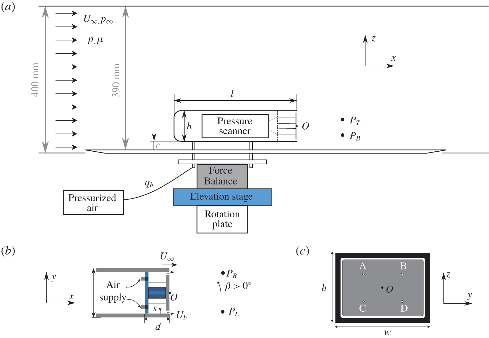
A three-dimensional body of length  $l=291~\text{mm}$, width
 $w=97.25~\text{mm}$ and height
 $h=72~\text{mm}$, whose geometry corresponds to the square-back model used by Ahmed, Ramm & Faltin (Reference Ahmed, Ramm and Faltin1984), is placed over a ground plate as shown in figure 1. It is held by four cylindrical supports of 7.5 mm diameter (i.e.
 $0.104h$), leaving a ground clearance of
 $c/h=0.278$. The model is mounted on a turntable to adjust the yaw angle
 $\unicode[STIX]{x1D6FD}$ of the body (rotation with respect to the
 $z$-axis) with an accuracy of
 $0.01^{\circ }$.
The rear of the body is constituted of a frame of depth  $d/h=0.417$ (see figure 1b) creating an internal cavity partially blocked at the base by a central plate. The plate is smaller than the cavity dimensions to leave a rectangular perimetric slit of width
 $s/h=0.028$ as depicted by the white rectangle in figure 1(c). The cavity is pressurized by injecting air through four internal tubes (sketched in figure 1b,c) with a steady controlled flow rate
 $q_{b}$. The velocity produced at the slit, denoted
 $U_{b}$, is illustrated in figure 1(a,b). The blowing system is connected to a 6 bar compressed air feeding line through a pneumatic tube with an Aalborg digital mass flow meter, an air valve and a pressure regulator, which ensures stability and constancy of the flow rate
 $q_{b}$.
(a) Sketch of the experimental set-up. (b) Top view of the body, showing the internal arrangement of the blowing system. (c) Rear view of the bluff body depicting the four pressure tap positions labelled A, B, C and D and the rectangular slit as the white rectangle. The labels  $P_{T}$,
 $P_{B}$,
 $P_{L}$ and
 $P_{R}$ in panels (a) and (b) indicate the locations for hot-wire measurements.

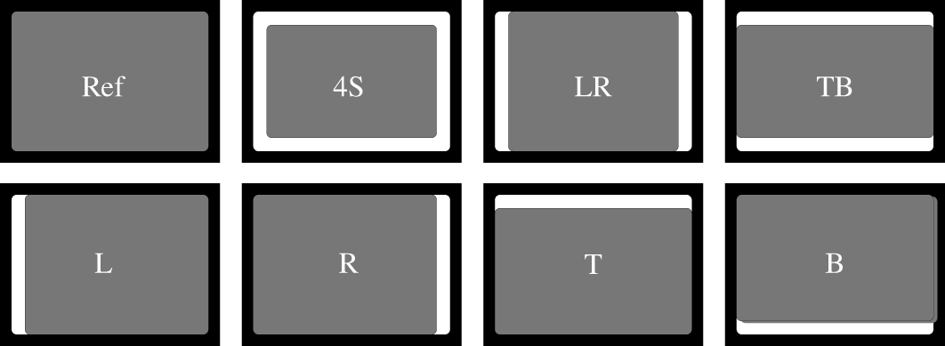
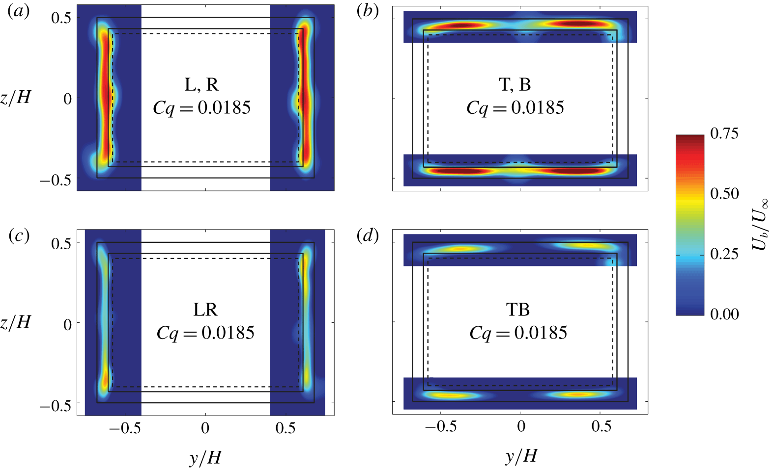
Seven blowing configurations shown in figure 2 are realized by partially blocking the rectangular slit by leaving open either one side (asymmetric configurations) or both opposite sides (symmetric configurations). The slits were blocked using aluminium tape placed on marked positions to assure repeatability. These configurations allow one to explore the sensitivity to different spatial distribution of blowing. The good symmetry properties of the injection is attested in figure 3 showing the velocity  $U_{b}$ along the active slits and in the absence of wind. The configurations are shown in figure 3: left (L), right (R), top (T) and bottom (B) for asymmetric configurations, and both left and right (LR), and both top and bottom (TB). As shown in figure 3, the lateral blowing configurations produce a nearly homogeneous profile. However, in the case of the top/bottom configurations, the blowing velocity is lower at the central part of the slit, although the velocity profiles are clearly symmetric in the longitudinal direction. Thus, the blowing inhomogeneity along a slit respects satisfactorily the reflectional symmetries of the rectangular base. Consequently, the blowing of the symmetric configurations is symmetric, and each blowing of the four asymmetric configurations only breaks the reflectional symmetry of the base as it has been designed for. The symmetric configuration corresponding to the full rectangular slit did not have the expected symmetry, and this configuration cannot be used as a spatially controlled disturbance of the wake mode. Nevertheless, a passive effect will be shown.
Sketch views of the rectangular base showing the reference case and the open slit configurations used for base blowing (see text). The open slits appear white on the rectangular base.

Contours of time-averaged blowing velocity obtained by means of hot-wire anemometry measurements at  $x/H=0.1$ and no wind for the six blowing configurations: (a) left (L) or right (R); (b) top (T) or bottom (B); (c) both left and right (LR), and (d) both top and bottom (TB). The non-dimensional blowing velocity is computed as
 $U_{b}/U_{\infty }$, where
 $U_{\infty }=20~\text{m}~\text{s}^{-1}$ will be the wind speed used for the remainder of the paper. For all configurations, the corresponding blowing coefficient is
 $C_{q}=0.0185$ (taking
 $U_{\infty }=20~\text{m}~\text{s}^{-1}$), which is the maximum value for the experiments.

The uniform wind is produced in an Eiffel-type wind tunnel with a three-quarters open jet facility of  $390~\text{mm}\times 400~\text{mm}$ aperture (identical to the facility of Grandemange et al. (Reference Grandemange, Gohlke and Cadot2013a)). The wind speed is fixed at
 $U_{\infty }=20~\text{m}~\text{s}^{-1}$, with a turbulent intensity below 0.5 % and a spatial inhomogeneity smaller than 0.3 %. The Reynolds number based on the height
 $h$ of the body is
 $Re=U_{\infty }h/\unicode[STIX]{x1D708}\approx 10^{5}$, where
 $\unicode[STIX]{x1D708}$ is the kinematic viscosity of air. The flow rate blowing coefficient is defined as
 $C_{q}=q_{b}/(U_{\infty }wh)$ and the velocity ratio blowing coefficient as
 $C_{u}=q_{b}/(U_{\infty }S_{b})$, where
 $S_{b}$ is the total blowing surface composed of the sum of the active slit surfaces. The maximum blowing coefficient investigated in the paper is
 $C_{q}=0.0185$, which corresponds to
 $C_{u}=1.1$ in the single lateral slit configuration.
The origin of the Cartesian coordinate system  $(x,y,z)$ is placed at the centre of the body base, with
 $x$ being the streamwise direction,
 $z$ the transverse direction normal to the ground, and
 $y$ the side direction that forms a direct trihedral. The velocity vector can therefore be decomposed into respective components
 $\boldsymbol{u}=(u_{x},u_{y},u_{z})$. The origin of the yaw angle is defined as in Evrard et al. (Reference Evrard, Cadot, Herbert, Ricot, Vigneron and Délery2016);
 $\unicode[STIX]{x1D6FD}=0$ corresponds to a bistable dynamics with equal probability of both deflected wake states. The difference from the geometrical alignment is
 $0.22^{\circ }$.
For the remainder of the paper,  $h$,
 $U_{\infty }$ and
 $h/U_{\infty }$ will be used as characteristic length, velocity and time scales, respectively. We denote with an asterisk
 $^{\ast }$ the dimensionless variables defined from these characteristic scales. Notation
 $St$, for Strouhal number, is used to designate a non-dimensional frequency using
 $h$ and
 $U_{\infty }$.
2.2 Pressure, velocity and force measurements
Pressure values are measured at four different locations  $(\,y^{\ast },z^{\ast })=(\pm 0.3,\pm 0.2)$ (indicated as A, B, C and D in figure 1c). A Scanivalve ZOC22 pressure scanner is placed inside the model, thus reducing the length of vinyl tubes required to connect the four pressure taps to the pressure sensor. The local pressures at the base are recorded at a sampling rate of 100 Hz each with an accuracy of
 $\pm 3.75~\text{Pa}$ and during 250 s for typical experiments. In the following, pressure will be expressed as instantaneous pressure coefficient
 $$\begin{eqnarray}\displaystyle c_{p}(\,y^{\ast },z^{\ast },t^{\ast })=\frac{p(\,y^{\ast },z^{\ast },t^{\ast })-p_{\infty }}{\unicode[STIX]{x1D70C}U_{\infty }^{2}/2}, & & \displaystyle\end{eqnarray}$$
where  $\unicode[STIX]{x1D70C}$ is the air density and
 $p_{\infty }$ is the reference static pressure at the inlet of the test section.
These four measurements are used to assess instantaneously the base drag and the wake asymmetry as introduced by Grandemange et al. (Reference Grandemange, Gohlke and Cadot2013b). In particular, such an arrangement can be considered a relevant minimal set of measurements to estimate accurately base drag and base pressure gradient. The reason is that the wall pressure distribution in the separated area is at first order almost constant in one direction and affine in the other perpendicular direction (direction of the asymmetry) as illustrated for different asymmetry directions by Barros et al. (Reference Barros, Borée, Cadot, Spohn and Noack2017). The drag is evaluated through the base drag or suction coefficient (Apelt & West Reference Apelt and West1975; Roshko Reference Roshko1993) calculated as
 $$\begin{eqnarray}\displaystyle c_{B}(t^{\ast })=-\frac{1}{4}\mathop{\sum }_{i=1}^{4}c_{p}(\,y_{i}^{\ast },z_{i}^{\ast },t^{\ast }). & & \displaystyle\end{eqnarray}$$
The precision on mean pressure coefficients, and then mean base drag, is estimated to be  $\pm 0.001$. The wake asymmetry, as previously satisfactorily investigated in Grandemange et al. (Reference Grandemange, Gohlke and Cadot2013a) and Bonnavion & Cadot (Reference Bonnavion and Cadot2018), is assessed by means of the non-dimensional base pressure gradient whose horizontal and vertical components,
 $g_{y}$ and
 $g_{z}$, are computed as
 $$\begin{eqnarray}\displaystyle & \displaystyle g_{y}={\displaystyle \frac{\unicode[STIX]{x2202}c_{p}}{\unicode[STIX]{x2202}y^{\ast }}}\simeq \frac{1}{2}\left[{\displaystyle \frac{c_{p}(\,y_{B}^{\ast },z_{B}^{\ast },t^{\ast })-c_{p}(\,y_{A}^{\ast },z_{A}^{\ast },t^{\ast })}{y_{B}^{\ast }-y_{A}^{\ast }}}+{\displaystyle \frac{c_{p}(\,y_{D}^{\ast },z_{D}^{\ast },t^{\ast })-c_{p}(\,y_{C}^{\ast },z_{C}^{\ast },t^{\ast })}{y_{D}^{\ast }-y_{C}^{\ast }}}\right]\!,\quad & \displaystyle\end{eqnarray}$$
 $$\begin{eqnarray}\displaystyle & \displaystyle g_{z}={\displaystyle \frac{\unicode[STIX]{x2202}c_{p}}{\unicode[STIX]{x2202}z^{\ast }}}\simeq \frac{1}{2}\left[{\displaystyle \frac{c_{p}(\,y_{A}^{\ast },z_{A}^{\ast },t^{\ast })-c_{p}(\,y_{C}^{\ast },z_{C}^{\ast },t^{\ast })}{z_{A}^{\ast }-z_{C}^{\ast }}}+{\displaystyle \frac{c_{p}(\,y_{B}^{\ast },z_{B}^{\ast },t^{\ast })-c_{p}(\,y_{D}^{\ast },z_{D}^{\ast },t^{\ast })}{z_{B}^{\ast }-z_{D}^{\ast }}}\right]\!.\quad & \displaystyle\end{eqnarray}$$
Polar coordinates are also a useful representation of the gradient, since the modulus  $g=\sqrt{g_{y}^{2}+g_{z}^{2}}$ is related to the strength of the wake asymmetry and the phase angle
 $\unicode[STIX]{x1D711}=\arccos (g_{y}/g)$ is related to its orientation. The mean pressure gradient precision deduced from that of the mean pressure coefficient given above is
 $\pm 0.003$ and
 $\pm 0.005$ for the
 $y$ and
 $z$ components, respectively.
In order to make accurate and repeatable base pressure measurements, we leave the wind tunnel working and the pressure scanner acquiring during approximately two hours before investigating one blowing configuration. Experiments are started when no drifts from the sensor signal are observed. We first acquire the non-blowing case, and then we increase by increments the blowing flow rate until the maximum value  $C_{q}=0.0185$, recording pressure signals for each selected blowing rate during 250 s. Once the series are achieved, a non-blowing case is again measured to remove any residual drift effects during the experiment. Direct measurements of the relative variation of the mean base drag,
 $\unicode[STIX]{x0394}C_{B}(C_{q})$, are therefore obtained by subtracting the mean base drag values of blowing,
 $C_{B}(C_{q})$, and corresponding non-blowing case of the selected configuration,
 $C_{B}(C_{q}=0)$. The protocol is repeated for all configurations. Base drag measurements with no blowing,
 $C_{B0}=C_{B}(C_{q}=0,U_{\infty })$, are realized separately where the mean value obtained with no wind is subtracted from the mean value with the wind.
Near-wake velocity fields in the two perpendicular planes  $y^{\ast }=0$ and
 $z^{\ast }=0$ are investigated to obtain, respectively, the fields
 $\boldsymbol{u}_{\boldsymbol{x}\boldsymbol{z}}^{\ast }=(u_{x}^{\ast },0,u_{z}^{\ast })$ and
 $\boldsymbol{u}_{\boldsymbol{x}\boldsymbol{y}}^{\ast }=(u_{x}^{\ast },u_{y}^{\ast },0)$ by means of particle image velocimetry (PIV) measurements. The PIV system uses a dual-pulse laser (Nd:YAG,
 $2\times 135~\text{mJ}$, 4 ns) synchronized with a FlowSense EO, 4 Mpx, charge-coupled device (CCD) camera. A camera resolution of
 $2360\times 1776$ pixels, in combination with a 35 mm focal length lens, allows us to cover a flow field extension of approximately
 $x^{\ast }\times y^{\ast }=[-0.5,3]\times [-1.3,1.3]$ and
 $x^{\ast }\times z^{\ast }=[-0.3,2.5]\times [-0.9,1.1]$ for measurements in the
 $z^{\ast }=0$ and
 $y^{\ast }=0$ planes, respectively, with corresponding pixel resolutions of
 $0.10~\text{mm}~\text{pixel}^{-1}$ and
 $0.08~\text{mm}~\text{pixel}^{-1}$. For typical measurements, 500 pairs of images (using a time delay of
 $50~\unicode[STIX]{x03BC}\text{s}$ between consecutive snapshots) at 10 Hz are acquired. The image masking, PIV image processing and post-processing of the velocity field obtained are performed using a standard PIV cross-correlation algorithm. Velocities are computed in two steps, using first an interrogation window of
 $32\times 32$ pixels, and then windows of
 $16\times 16$ pixels, in both cases with an overlap of
 $50\,\%$. By using this window size, a mesh of
 $295\times 222$ points for both PIV plane locations was obtained, resulting in a spatial resolution of
 $\unicode[STIX]{x0394}x=\unicode[STIX]{x0394}y=0.8~\text{mm}$ (
 $0.011h$) and
 $\unicode[STIX]{x0394}x=\unicode[STIX]{x0394}z=0.64~\text{mm}$ (
 $0.009h$) for planes
 $z=0$ and
 $y=0$, respectively.
The PIV system is supplemented with a single hot-wire probe placed further downstream to provide the frequency of the global periodic wake modes. Four measurement locations are investigated; they are shown in figure 1 denoted by  $P_{L}=(x^{\ast }=2.5,y^{\ast }=-0.5,z^{\ast }=0)$,
 $P_{T}=(2.5,0,0.3)$,
 $P_{R}=(2.5,0.5,0)$ and
 $P_{B}=(2.5,0,-0.3)$. The wire is oriented in such a way as to measure the modulus
 $u_{xz}$ for the vertical positions at
 $P_{T}$ and
 $P_{B}$ and the modulus
 $u_{yz}$ for the lateral positions at
 $P_{L}$ and
 $P_{R}$. The hot-wire measurements are sampled at 1 kHz and dominant frequencies are extracted from the power spectral density (PSD), computed using sliding windows of 2 s over a signal duration of 120 s, which resulted in a frequency resolution of 0.5 Hz.
The aerodynamic force exerted on the body is measured with a multi-axial load cell (model AMTI-MC3A-100lb) connected to the four cylindrical supports (see figure 1). Time series of drag, side and lift components, i.e.  $f_{x}$,
 $f_{y}$ and
 $f_{z}$, respectively, are recorded during 60 s at a sampling rate of 1 kHz. The uncertainty of the measurements is estimated (using specifications of crosstalk, nonlinearity and hysteresis) to be 0.002 N for the
 $x$ and
 $y$ directions and 0.006 N for the
 $z$ direction, due to its bigger range. The drag, side and lift coefficients are defined as
 $$\begin{eqnarray}\displaystyle c_{i}=\frac{f_{i}}{hw\unicode[STIX]{x1D70C}U_{\infty }^{2}/2}, & & \displaystyle\end{eqnarray}$$
with a corresponding uncertainty of approximately  $\pm 0.001$ for
 $c_{x}$ and
 $c_{y}$ and of
 $\pm 0.003$ for
 $c_{z}$.
Since we are interested in values without the thrust and slits head loss produced by the blowing itself, we subtract from the mean force  $F_{i}=F_{i}(C_{q},U_{\infty })$ obtained for a given blowing and wind speed, the mean force at the same blowing but with no wind
 $F_{i}(C_{q},U_{\infty }=0)$. Thus, the mean value
 $$\begin{eqnarray}\displaystyle \tilde{C}_{i}=\frac{F_{i}(C_{q},U_{\infty })-F_{i}(C_{q},U_{\infty }=0)}{hw\unicode[STIX]{x1D70C}U_{\infty }^{2}/2} & & \displaystyle\end{eqnarray}$$
is assumed to be the force coefficient when blowing jet effects are removed. For accurate measurements of  $\tilde{C}_{i}$, we operate as follows. For each
 $C_{q}$ and in a single acquisition run, we measure with blowing alone for 15 s (wind tunnel switched off), we then turn on the wind tunnel to capture 30 s of aerodynamic force, and stop the wind tunnel to measure again with blowing alone for another 15 s. Taking the average of the two blowing-alone stages, and subtracting from the mean force measured during 30 s, we obtain
 $\tilde{C}_{i}$. Measurements of
 $C_{i}$ with no blowing are realized separately where the mean value obtained with no wind is subtracted from the mean value with the wind.
Conditional statistics are realized on any measurements presented above to extract the characteristics of the  $P$ or
 $N$ state (Grandemange et al. Reference Grandemange, Gohlke and Cadot2013b). They correspond to events such that the horizontal component of the pressure gradient
 $g_{y}>0$ (for
 $P$ state) or
 $g_{y}<0$ (for
 $N$ state). For the remainder of the paper, we will denote by a superscript
 $P$ or
 $N$ the conditional averaging of any variables following this rule. Pressure is always simultaneously recorded with the PIV measurements to proceed for conditional averaging on the velocity fields.
The following notation is used: time-dependent variables are denoted by lower-case letters  $a$, time-averaged values by upper-case letters
 $A=\overline{a}$ and standard deviations by
 $A^{\prime }=\sqrt{\overline{(a-A)^{2}}}$. As defined previously, conditional statistics denoted
 $A^{i}$ and
 ${A^{\prime }}^{i}$ are, respectively, the average and standard deviation of the
 $i=P$ or
 $N$ state. We will use the notation
 $A_{0}=A(C_{q}=0)$ for measurements with no blowing and
 $\unicode[STIX]{x0394}A$ for a difference from the non-blowing case:
 $\unicode[STIX]{x0394}A=A(C_{q})-A_{0}$.
3 Results
We now present the flow at  $Re=10^{5}$. This results section is organized as follows. It starts with a preliminary characterization of the reference case (no slits) and then takes into account the different configurations of open slits without blowing in § 3.1. Two regimes of blowing referred to as mass and momentum are evidenced in § 3.2 on the basis of base drag measurements. The detailed investigations of the wake focusing on the static symmetry-breaking modes is in § 3.3 and then on the periodic modes is in § 3.4. The path of the injected mass is assessed for the two blowing regimes in § 3.5 and, finally, § 3.6 characterizes the correlation of the recirculating length and the base drag.
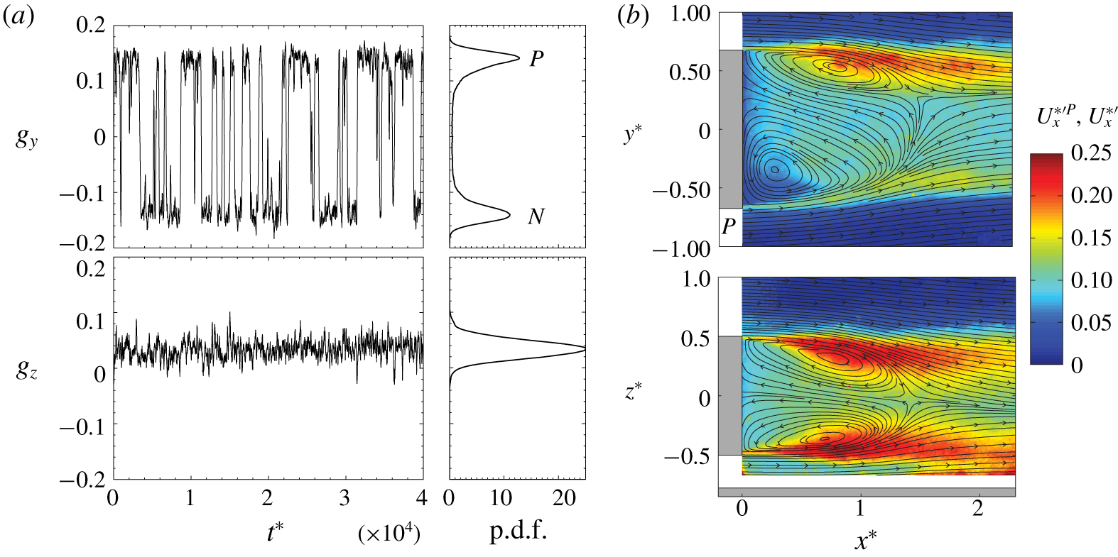
Reference case (no slits). (a) Time series of the pressure gradient components  $g_{y}(t^{\ast })$ and
 $g_{z}(t^{\ast })$ and their corresponding p.d.f. (b) Streamlines of the mean velocity field
 $\boldsymbol{U}_{\boldsymbol{x}\boldsymbol{y}}^{\ast P}$ (top) and
 $\boldsymbol{U}_{\boldsymbol{x}\boldsymbol{z}}^{\ast }$ (bottom) superimposed on the velocity fluctuations
 $U_{x}^{\ast ^{\prime }P}$ (top) and
 $U_{x}^{\ast ^{\prime }}$ (bottom).

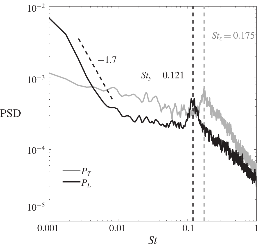
Reference case (no slits). The PSD of the local velocity at  $P_{T}$ and
 $P_{L}$ (see figure 1). The resonant peaks indicate the presence of the periodic asymmetric modes of the wake with a high frequency
 $St_{z}=0.175$ for the vertical mode and a low frequency
 $St_{y}=0.121$ for the horizontal mode (Grandemange et al. Reference Grandemange, Gohlke and Cadot2013a).

3.1 Flow without blowing
The wake of the body with the additional rear device without open slits at the base is referred to as the reference case. It exhibits the well-known long-time bistable dynamics due to the  $y$-instability as reported in Grandemange et al. (Reference Grandemange, Gohlke and Cadot2013a,Reference Grandemange, Gohlke and Cadotb). This behaviour is clearly observed by the random switches of the horizontal component of the pressure gradient
 $g_{y}$ in figure 4(a). They occur between two well-defined mirrored states denoted
 $P$ and
 $N$ in the corresponding probability density function (p.d.f.). The time spent in one state can be as large as a few orders of magnitudes of the convective time scale. The vertical component of the pressure gradient
 $g_{z}$ remains almost insensitive to the switching dynamics in figure 4(a). Its positive value is introduced by the presence of the body support and the ground. The wake topology corresponding to the
 $P$ state is obtained in figure 4(b) and reveals the static mode of the wake as reported in the literature. The
 $N$ state (not shown here) is a mirror symmetry (
 $y^{\ast }\rightarrow -y^{\ast }$) of the
 $P$ state.
Reference case (no slits). Mean values of force coefficients, base drag, recirculating bubble length, base pressure gradient modulus of the static mode with components for its  $N$ and
 $P$ states, Strouhal numbers of the periodic modes.

The two periodic modes of the wake are identified in the PSD shown in figure 5 of the local velocity measurements in the wake. In accordance with the wake characterization of Grandemange et al. (Reference Grandemange, Gohlke and Cadot2013a), we find a low resonant frequency denoted  $St_{y}=0.121$ (captured by the local velocity at
 $P_{L}$) associated with the global lateral motion and a high resonant frequency denoted
 $St_{z}=0.175$ (captured by the local velocity at
 $P_{T}$) associated with the global vertical motion. In addition, the random bistable dynamics in the horizontal direction can be identified in the PSD of
 $P_{L}$ with the
 $-1.7$ decay for low values of
 $St$.
Table 1 summarizes the main global flow characteristics of the reference case such as force coefficients, recirculating bubble length, base drag and mean pressure gradient. Recirculation region extension has been characterized as the maximum downstream location from the body base where  $U_{x}^{\ast }\leqslant 0$. All these values are in accordance with previous measurements for similar square-back geometries. However, strict comparison with other published works is meaningless because none of the geometries are identical, with significant variations such as fore-body shape, support design, ground clearance and body dimensions. In this regard, the present drag coefficient
 $C_{x}^{Ref}=0.371$ obtained with a body length
 $l^{\ast }=4$ and a ground clearance
 $c^{\ast }=0.278$ is substantially larger than the
 $C_{x}=0.274$ obtained by Grandemange et al. (Reference Grandemange, Gohlke and Cadot2013a) with a body length
 $l^{\ast }=3.6$ and a ground clearance
 $c^{\ast }=0.174$. It is worth mentioning that for both cases the base drag is similar,
 $C_{B}=0.177$ in the present case and
 $C_{B}=0.185$ in Grandemange et al. (Reference Grandemange, Gohlke and Cadot2013a). The drag discrepancy can be reasonably explained by the additional length of the cylindrical supports together with the friction introduced by the body extension. We can see in table 1 that the floor and supports produce a negative lift coefficient
 $C_{z}=-0.055$; the bistable dynamics between the two asymmetric states is responsible for the large fluctuation in the side force coefficient
 $C_{y}^{\prime }=0.019$ due to the random switches of the
 $y$ component of pressure gradient between the mean values of both states
 $G_{y}^{N,Ref}$ and
 $G_{y}^{P,Ref}$. The mean pressure gradient modulus
 $G^{Ref}=0.133$ gives the strength of the permanent wake asymmetry.
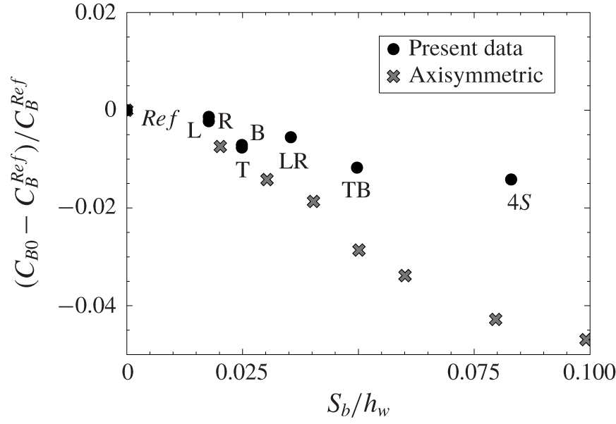
Base drag modification for all slit configurations as displayed in figure 2 without blowing versus slit area. The axisymmetric data are from García de la Cruz, Oxlade & Morrison (Reference García de la Cruz, Oxlade and Morrison2017).

We denote by  $C_{B0}$ the base drag obtained for each slit configuration as displayed in figure 2 without injection, i.e.
 $C_{q}=0$. Whatever the configuration, a slight reduction of
 $C_{B0}$ is obtained from the reference case. This effect due to open slits at the base was also found by Bearman (Reference Bearman1967) for a two-dimensional blunt body and by García de la Cruz et al. (Reference García de la Cruz, Oxlade and Morrison2017) for an axisymmetric blunt body. The relative change of base drag coefficient
 $(C_{B0}-C_{B}^{Ref})/C_{B}^{Ref}$ is shown in figure 6 against the slit area normalized by the base area,
 $S_{b}/hw$. The decrease obtained by García de la Cruz et al. (Reference García de la Cruz, Oxlade and Morrison2017) with a perimetric slit on a circular base is also reported in figure 6. The rectangular perimetric slit (configuration 4S) is shown for comparison with the circular perimetric slit. A much smaller relative base drag decrease is observed with the wake of the rectangular base that is approximately
 $1.5\,\%$ compared to the
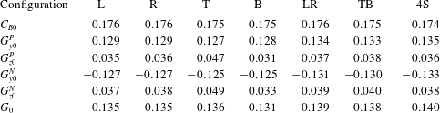
 $4\,\%$ of the circular base. This reduction is interpreted in García de la Cruz et al. (Reference García de la Cruz, Oxlade and Morrison2017) as an effect associated with a decrease of the intensity of the wake asymmetry and likely to be produced by the stabilization of the static mode. In order to check this result in our geometry, table 2 shows base drag and mean pressure gradients for all configurations. It appears that, as a general trend in our accuracy, the asymmetry strength given by
 $G_{0}$ is rather increased in comparison to the reference value of 0.133 with open slits. However, according to the precision of
 $\pm 0.005$ for the mean pressure gradient and
 $\pm 0.001$ for the base drag, these weak effects seem unfortunately at the limit of our measurements, which may lead to unreliable conclusions. A significant effect, however, is detectable on the
 $z$ component of the pressure gradient for B and T configurations pointing out a local pressure increase on the side of the open slit thus enhancing the vertical component in the T configuration and reducing it in the B configuration.
Passive effect values ( $C_{q}=0$) for all configurations.

3.2 Blowing effect on the base drag
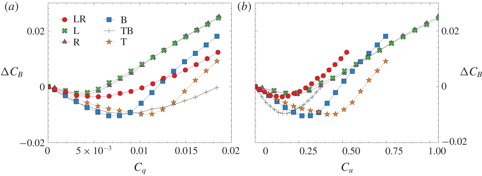
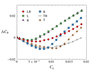
The base drag variation  $\unicode[STIX]{x0394}C_{B}=C_{B}-C_{B0}$ is shown for all configurations as a function of
 $C_{q}$ in figure 7(a) and
 $C_{u}$ in figure 7(b). We recall that the L and R configurations are symmetrically equivalent, explaining why the corresponding curves are superimposed.
Base drag coefficient variation  $\unicode[STIX]{x0394}C_{B}=C_{B}-C_{B0}$ versus (a) the flow rate coefficient
 $C_{q}$ and (b) the blowing velocity ratio
 $C_{u}$.

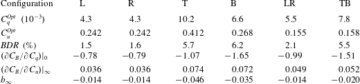
Data extracted from figure 7. Optimal values of base bleed coefficients for maximum base drag reduction  $BDR=-\unicode[STIX]{x0394}C_{B}^{min}/C_{B0}$ for all configurations. Parameters of the linear fit in the mass regime,
 $\unicode[STIX]{x0394}C_{B}=(\unicode[STIX]{x2202}C_{B}/\unicode[STIX]{x2202}C_{q})|_{0}C_{q}$, and in the momentum regime,
 $\unicode[STIX]{x0394}C_{B}=(\unicode[STIX]{x2202}C_{B}/\unicode[STIX]{x2202}C_{u})|_{\infty }C_{u}+b_{\infty }$.

The same trend is observed for all configurations, characterized by an initial base drag reduction with increasing values of the blowing intensity, followed by a constant-slope increase of base drag. This general behaviour is similar to that obtained by Wood (Reference Wood1964) for two-dimensional bodies implementing rear blowing. Two blowing regimes have to be distinguished: we will refer to these as the mass regime, the small blowing for which the base drag is decreased; and the momentum regime, the larger blowing for which the base drag is increased. Both regimes are fitted with linear regressions whose parameters are given in table 3.
The maximum of base drag reduction,  $BDR$ (approximately from
 $1\,\%$ to
 $7\,\%$), and the corresponding optimal blowing coefficients,
 $C_{q}^{Opt}$ and
 $C_{u}^{Opt}$, summarized in table 3, show a substantial dependence on the blowing configuration. Maximal reductions involve the top or bottom slits whether the configuration is symmetric or not. The B configuration achieves the best reduction. There is no evidence of a simple relation between either the optimal
 $C_{q}$ or
 $C_{u}$ and the blowing configurations. This high and non-trivial sensitivity to the blowing location and intensity is investigated in the next sections by studying the interaction of the wake modes with the blowing.
3.3 Static mode
3.3.1 Asymmetric blowing configurations
The two configurations L and R have been investigated identically and the experimental data are, as expected, symmetrically equivalent. For brevity of the paper, we only present results for one configuration, and the results for the other can be deduced by the left to right reflectional symmetry.
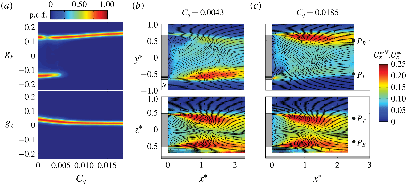
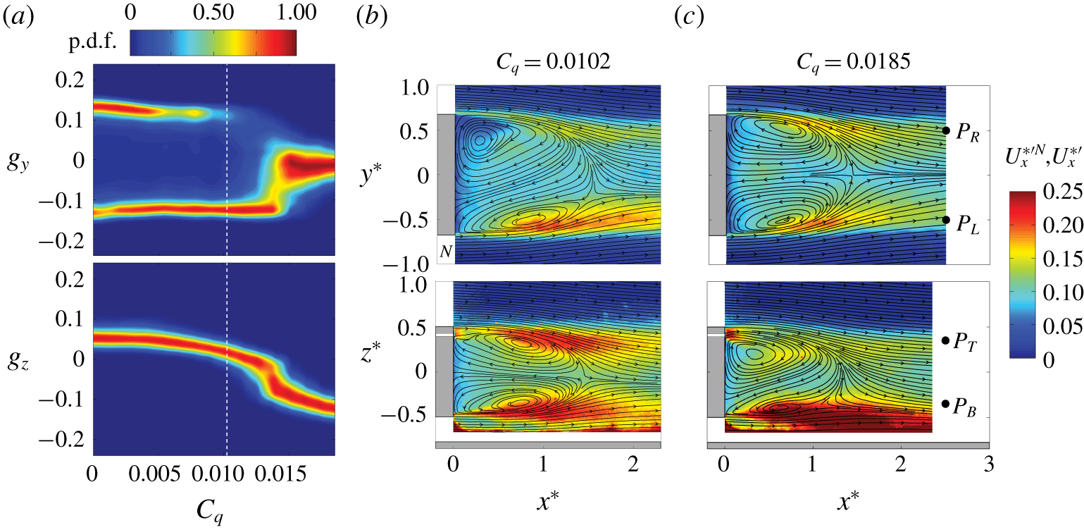
Blowing in L configuration. (a) Sensitivity maps of the Cartesian components,  $g_{y}$ and
 $g_{z}$, of the base pressure gradient. The white dashed line marks the
 $C_{q}^{Opt}$ value for which the mean base drag
 $C_{B}$ is minimum. (b,c) Streamlines of the mean velocity field
 $\boldsymbol{U}_{\boldsymbol{x}\boldsymbol{y}}^{\ast N}$ (top, left),
 $\boldsymbol{U}_{\boldsymbol{x}\boldsymbol{y}}$ (top, right) and
 $\boldsymbol{U}_{\boldsymbol{x}\boldsymbol{z}}^{\ast }$ (bottom) superimposed on their corresponding velocity fluctuations
 $U_{x}^{\ast ^{\prime }N}$ or
 $U_{x}^{\ast ^{\prime }}$ for (b)
 $C_{q}^{Opt}=0.0043$ and (c)
 $C_{q}=0.0185$. The white bands in (b) and (c) indicate the blowing slits.

The sensitivity map of the Cartesian components of the base pressure gradient for the L configuration is displayed in figure 8(a). As introduced in Bonnavion & Cadot (Reference Bonnavion and Cadot2018), it represents the p.d.f. of the gradient component normalized by the most probable value computed from each value of the varying parameter, here the blowing flow rate. The vertical dashed line locates the optimal value of blowing that separates the mass and momentum regime as defined above. The positive (respectively negative) branch corresponds to the  $P$ state (respectively
 $N$ state). In the mass regime,
 $C_{q}<C_{q}^{Opt}$, the dynamics is bistable, involving both
 $P$ and
 $N$ states. From the initial case at
 $C_{q}=0$ where both states are equiprobable, we see a significant change in their probability of presence as blowing is increased, promoting the
 $N$ state. The preferential state selection in the mass regime is then opposite to that of the momentum regime. It can be seen that the change of blowing regime is accompanied with a permanent wake reversal towards the
 $P$ state (figure 8c) that was predominantly in the
 $N$ state (figure 8b) in the mass regime. The momentum regime is then associated with a selected
 $P$ state in L configuration, where the blowing jet (clearly identified by its large localized fluctuation
 $U_{x}^{\ast ^{\prime }}$ in front of the slit) is fixing the steady circular recirculation of the bubble. It is also worth mentioning that there is almost no trace of the blowing jet for the largest blowing in the mass regime reached when
 $C_{q}=C_{q}^{Opt}$ in figure 8(b). However, a direct effect of the blowing can be identified through the additional linear increase of
 $g_{y}$ in figure 8(a). The blowing is likely to produce a positive pressure gradient proportional to
 $C_{q}$ that is not affected by the wake state whether it is
 $P$ or
 $N$.
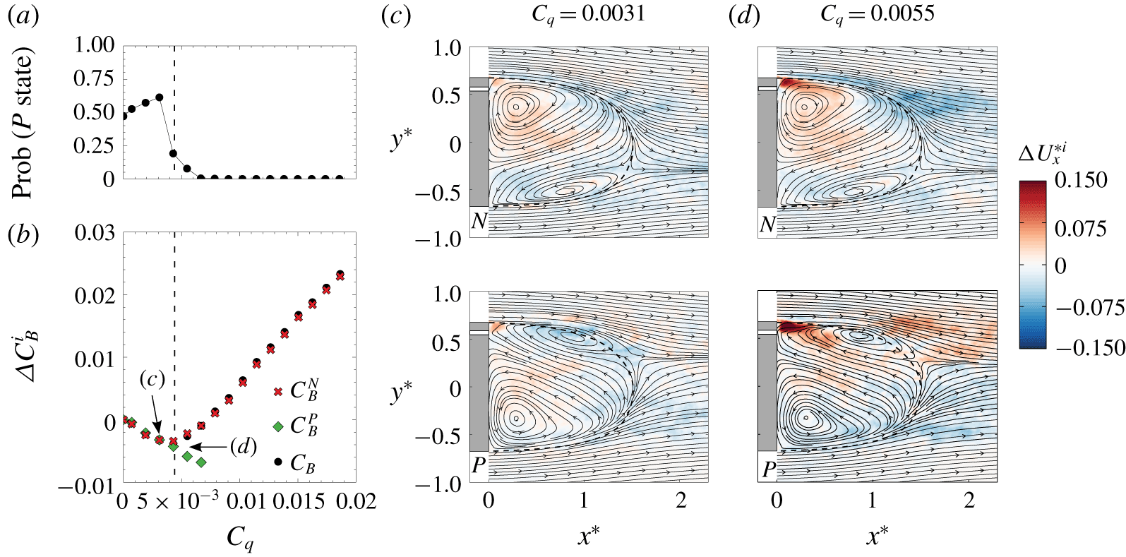
Blowing in R configuration. (a) Probability of occurrence of the  $P$ state and (b) relative variation of base drag for
 $N$ and
 $P$ states versus the blowing coefficient. The dashed line marks the
 $C_{q}^{Opt}$ value for which
 $C_{B}$ is minimum. (c,d) Contours of the mean streamwise velocity difference
 $\unicode[STIX]{x0394}U_{x}^{\ast i}=U_{x}^{\ast i}-U_{x0}^{\ast i}$ of states
 $i=P,N$ superimposed on the mean flow streamlines of the field
 $\boldsymbol{U}_{\boldsymbol{x}\boldsymbol{y}}^{\ast i}$ for (c)
 $C_{q}=0.0031$ and (d)
 $C_{q}=0.0055$. White bands in (c) and (d) indicate the blowing slits.

We now turn to the effect of the L or R blowing during the bistable dynamics. Actually, there should be a distinction whether the wake is in an  $N$ or
 $P$ state. Depending on the wake state, the jet blows in either an opposite streamwise velocity region as depicted in figure 8(b, top), or in an adverse streamwise velocity region as depicted in figure 8(c, top). Conditional averaging is thus performed next to distinguish the two cases.
Figure 9 presents results obtained with configuration R. During the bistable dynamics that extend until  $C_{q}=6.6\times 10^{-3}$ in figure 9(a), the mass regime preferentially selects the
 $P$ state with a probability larger than 0.5 while the momentum regime selects the
 $N$ state. These are actually the expected results for the R configuration, which can be deduced from the mirror symmetry of the above observations concerning the L configuration described in figure 8. The mean base drag and mean velocity field of each state are respectively shown in figure 9(b) and figure 9(c,d). There is no distinction in the base drag of the two states until the blowing coefficient reaches
 $C_{q}=C_{q}^{Opt}$. Bistable dynamics occur as far as the
 $P$ state is observable, which extends beyond
 $C_{q}^{Opt}$ until
 $C_{q}=6.6\times 10^{-3}$. Around this blowing limit, the velocity fields displayed by the streamlines of the two states in figure 9(d) are globally mirrored by each other, while the corresponding base drag reductions are significantly different. The
 $P$ state is likely to be in a mass regime with a base drag reduction that is still increasing linearly with the blowing coefficient, while the
 $N$ state produces a base drag increase characteristic of the momentum regime. We deduce that it is more favourable for base drag reduction to blow in the opposite velocity flow region than in the adverse velocity region. Since the blowing jet is hardly discernible in the mean flows, we superimposed on the streamlines in figure 9(c,d) the difference of the mean streamwise velocity with that of the flow at
 $C_{q}=0$, say
 $\unicode[STIX]{x0394}U_{x}^{\ast i}=U_{x}^{\ast i}-U_{x0}^{\ast i}$, where
 $i=P$ or
 $N$ denotes the state. The blowing jet is not discernible in the mass regime in figure 9(c) for both states at
 $C_{q}=0.0031$, indicating that the injected momentum is efficiently mixed (i.e. dissipated) in the asymmetric recirculating bubble independently of the injection location. On the other hand, the jet is clearly observable in figure 9(d) at
 $C_{q}=0.0055$. For both states it contributes to increase the momentum, obviously more when located in the opposite flow region in the
 $P$ state in figure 9(
 $d$, bottom) than in the
 $N$ state in figure 9(
 $d$, top).
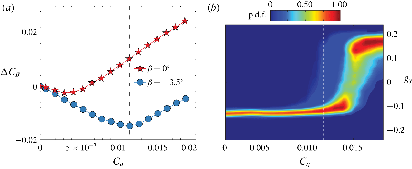
Blowing in L configuration with yaw. (a) Relative variation of base drag versus the injection coefficient for the body yawed at  $\unicode[STIX]{x1D6FD}=-3.5^{\circ }$. The case
 $\unicode[STIX]{x1D6FD}=0^{\circ }$ is added for comparison. (b) Sensitivity map of the horizontal component of the base pressure gradient to blowing with the yaw
 $\unicode[STIX]{x1D6FD}=-3.5^{\circ }$. In (b) and (c), the dashed line marks
 $C_{q}^{Opt}=0.0115$ for which the mean base drag
 $C_{B}$ is minimum.

The favourable configuration (injection in the reversed flow region of the bubble) can be forced by applying a yaw angle  $\unicode[STIX]{x1D6FD}$ to the body. It has been previously shown (Volpe, Devinant & Kourta Reference Volpe, Devinant and Kourta2015) that a yaw of
 $1^{\circ }$ is sufficient to permanently select a
 $P$ (respectively
 $N$) state with a positive (respectively negative) yaw without any modification of the base pressure gradient modulus (Bonnavion & Cadot Reference Bonnavion and Cadot2018). Figure 10(a) shows the base pressure variation where the body has been yawed to
 $\unicode[STIX]{x1D6FD}=-3.5^{\circ }$ to select an
 $N$ state. As expected, the mass regime is extended by a blowing in the L configuration compared to the unforced wake (
 $\unicode[STIX]{x1D6FD}=0^{\circ }$). It reaches a larger limit value
 $C_{q}^{Opt}=0.0115$ and an increased maximum base drag reduction of
 $7.5\,\%$. The sensitivity map of the horizontal component of the pressure gradient shows that, in the mass regime, the gradient magnitude of the forced
 $N$ state remains unchanged until bistable dynamics appear due to the compensation effect (Bonnavion & Cadot Reference Bonnavion and Cadot2018) of asymmetries between yaw and local momentum injection at the base.
Blowing in T configuration. (a) Sensitivity maps of the Cartesian components,  $g_{y}$ and
 $g_{z}$, of the base pressure gradient. The white dashed line marks the
 $C_{q}^{Opt}$ value for which the mean base drag
 $C_{B}$ is minimum. (b,c) Streamlines of the mean velocity field
 $\boldsymbol{U}_{\boldsymbol{x}\boldsymbol{y}}^{\ast N}$ (top, left),
 $\boldsymbol{U}_{\boldsymbol{x}\boldsymbol{y}}$ (top, right) and
 $\boldsymbol{U}_{\boldsymbol{x}\boldsymbol{z}}^{\ast }$ (bottom) superimposed on their corresponding velocity fluctuations
 $U_{x}^{\ast ^{\prime }N}$ or
 $U_{x}^{\ast ^{\prime }}$ for (b)
 $C_{q}^{Opt}=0.0102$ and (c)
 $C_{q}=0.0185$. The white bands in (b) and (c) indicate the blowing slit.

The L or R blowing configuration studied above breaks the same symmetry as the static modes (i.e. left/right symmetry), leading in the momentum regime to the permanent selection of a unique state. Now, we investigate B or T blowing configurations that break the top/bottom symmetry and will show very different interaction with the wake. The sensitivity map of the base pressure gradient in the T configuration is shown in figure 11(a). A bistable dynamics is observed during the entire mass regime. At the maximum of drag reduction, the wake topology (figure 11b) remains very similar to that of the reference flow. The momentum regime is first marked by the disappearance of the  $P$ state and then the suppression of the asymmetry in the
 $y$ direction since the horizontal component
 $g_{y}$ eventually fluctuates around a unique value equal to zero. This suppression is simultaneously accompanied by a decrease of the gradient component
 $g_{z}$ in the
 $z$ direction. It indicates that the blowing at the upper part of the base has rotated the two states to a single state with a vertical asymmetry leading to an
 $N$ state in the
 $z$ direction. This is clearly illustrated by the velocity fields in figure 11(c) for the largest blowing coefficient. The
 $N$ state in the
 $z$ direction that is forced by blowing in the T configuration actually reproduces the same situation as observed in the momentum regime (figure 8c) with the
 $P$ state in the
 $y$ direction selected by blowing in the L configuration. These two cases are deduced from each other by a simple
 $\unicode[STIX]{x03C0}/2$ rotation.
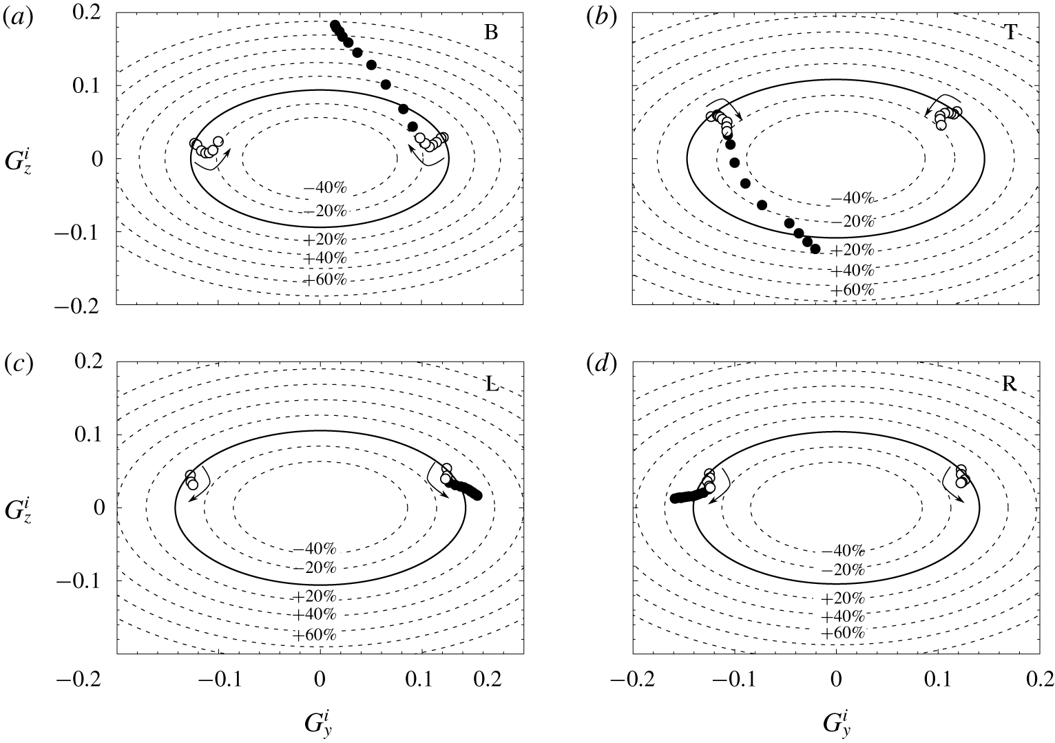
Blowing in asymmetric configurations: (a) T, (b) B, (c) L and (d) R. Mean pressure gradient components of the wake states  $(G_{y}^{i},G_{z}^{i})$ with
 $i=N,P$ in mass regime (empty symbols) and momentum regime (filled symbols). The solid line ellipse is the model of Bonnavion & Cadot (Reference Bonnavion and Cadot2018) (see text) and dashed ellipses stand for variations of
 $20\,\%$ of the gradient magnitude obtained with no blowing. The arrows indicate gradual increase of the blowing coefficient
 $C_{q}$.

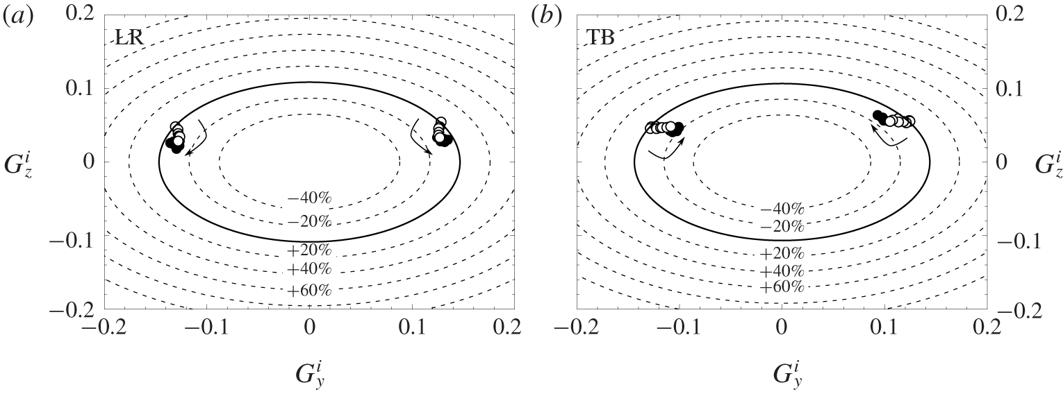
The gradual rotation of the base pressure gradient as the blowing is increased is better quantified in figure 12, which summarizes the base pressure gradient evolution for all asymmetric blowing configurations. Each point of the plot represents the mean gradient of a corresponding wake state, either  $P$ or
 $N$, obtained through conditional averaging. By definition, the
 $P$ branch develops on the right-hand side of the plot and the
 $N$ branch on the left-hand side. The continuous ellipse is modelling all the possible pressure gradients of the unstable wake (i.e. dominated by a static mode) that would have been passively selected by steady disturbances of pitch and yaw of the body in the absence of blowing (Bonnavion & Cadot Reference Bonnavion and Cadot2018). This view gives useful information about the wake asymmetry strength measured as the modulus of the gradient. Gradients located on the initial ellipse indicate no modification of the asymmetry strength compared to that naturally developed by the body geometry. However, when the blowing is activated, the wake strength is modified and gradients locate in different magnitude levels, as illustrated in figure 12 (see dashed ellipses), where the arrows represent the gradual increase of the blowing coefficient
 $C_{q}$. In particular, the mass regime (empty symbols) in the T and B configurations in figure 12(a,b) leads to a decrease of 20 % of the initial mean gradient modulus. However, the momentum regime (filled symbols) in which the rotation occurs shows a significant amplification of the asymmetry likely to be fed by the blowing jet. The same representation of the gradient of the wake states for the L and R blowing configuration (figure 12c,d) indicates as well an attenuation of the asymmetry during the mass regime (approximately 10 %) and an amplification in the momentum regime. The reduction of the asymmetry is mainly ascribed to a decrease of the horizontal component of the gradient for B or T configurations and of the vertical component for L or R configurations.
3.3.2 Symmetric blowing configurations
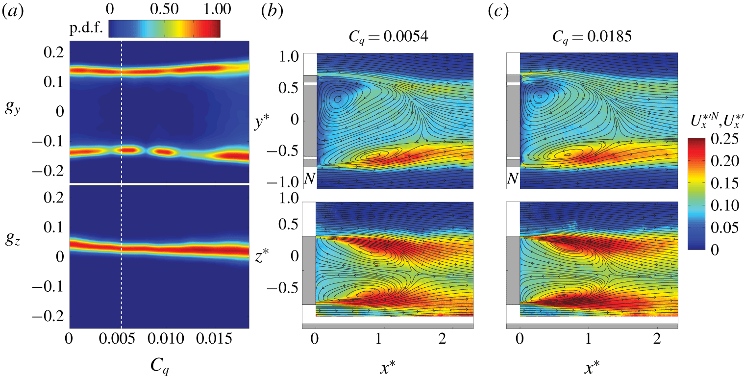
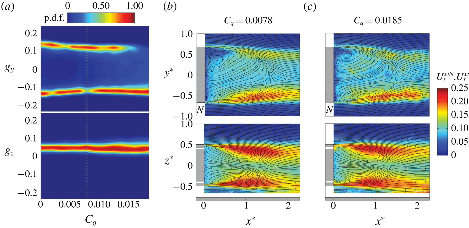
The two symmetric configurations, obtained with a simultaneous blowing in either the left and right slits (LR) or top and bottom slits (TB), give very similar results. The sensitivity maps of the base pressure gradient, respectively given in figure 13(a) and figure 14(a), indicate that bistable dynamics are conserved as expected by the blowing symmetry. The two  $P$ and
 $N$ states remain also very similar whatever the blowing injection is, as can be seen in figures 13(b,c) and 14(b,c). However, the horizontal gradient component
 $g_{y}$ reaches a small value for the optimal blowing coefficient in both figures 13(a) and 14(a), showing that maximum base drag reduction is associated with a strength reduction of the asymmetry.
Blowing in LR configuration. (a) Sensitivity maps of the Cartesian components,  $g_{y}$ and
 $g_{z}$, of the base pressure gradient. The white dashed line marks the
 $C_{q}^{Opt}$ value for which the mean base drag
 $C_{B}$ is minimum. (b,c) Streamlines of the mean velocity field
 $\boldsymbol{U}_{\boldsymbol{x}\boldsymbol{y}}^{\ast N}$ (top) and
 $\boldsymbol{U}_{\boldsymbol{x}\boldsymbol{z}}^{\ast }$ (bottom) superimposed on their corresponding velocity fluctuations
 $U_{x}^{\ast ^{\prime }N}$ or
 $U_{x}^{\ast ^{\prime }}$ for (b)
 $C_{q}^{Opt}=0.0054$ and (c)
 $C_{q}=0.0185$. The white bands in (b) and (c) indicate the blowing slits.

Blowing in TB configuration. (a) Sensitivity maps of the Cartesian components,  $g_{y}$ and
 $g_{z}$, of the base pressure gradient. The white dashed line marks the
 $C_{q}^{Opt}$ value for which the mean base drag
 $C_{B}$ is minimum. (b,c) Streamlines of the mean velocity field
 $\boldsymbol{U}_{\boldsymbol{x}\boldsymbol{y}}^{\ast N}$ (top) and
 $\boldsymbol{U}_{\boldsymbol{x}\boldsymbol{z}}^{\ast }$ (bottom) superimposed on their corresponding velocity fluctuations
 $U_{x}^{\ast ^{\prime }N}$ or
 $U_{x}^{\ast ^{\prime }}$ for (b)
 $C_{q}^{Opt}=0.0078$ and (c)
 $C_{q}=0.0185$. The white bands in (b) and (c) indicate the blowing slits.

Figure 15 recaps the base pressure gradient evolution for the two symmetric blowings. We observe an attenuation of the asymmetry strength given by the mean gradient modulus of approximately 10 % for the LR configuration mainly caused by a decrease of the vertical component and 20 % for the TB configuration due to a decrease of the horizontal component.
Blowing in symmetric configurations: (a) LR and (b) TB. Mean pressure gradient components of the wake states  $(G_{y}^{i},G_{z}^{i})$ with
 $i=N,P$ in mass regime (empty symbols) and momentum regime (filled symbols). The solid line ellipse is the model of Bonnavion & Cadot (Reference Bonnavion and Cadot2018) (see text commenting on figure 12) and dashed ellipses stand for variations of
 $20\,\%$ of the gradient magnitude obtained with no blowing. The arrows indicate the gradual increase of the blowing coefficient
 $C_{q}$.

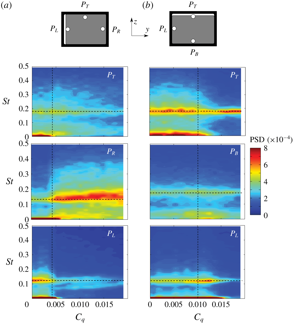
Effect of blowing on the wake periodic modes in (a) L and (b) T configurations. Contours of PSD of local velocity measured at  $P_{L}$,
 $P_{R}$,
 $P_{T}$ and
 $P_{B}$ (see § 2.2) as depicted at the top of the figure and also in figures 8 and 11. The horizontal dashed lines are the values of the Strouhal numbers,
 $St_{y}=0.121$ and
 $St_{z}=0.175$, of the reference case. The vertical dashed lines mark the
 $C_{q}^{Opt}$ value for which the mean base drag
 $C_{B}$ is minimum.

3.4 Periodic modes
Here, the global periodic modes are studied for steady blowing using the L and T blowing configurations only, each by means of three local point velocity measurements in the wake. Their locations (see § 2.2) are displayed in figure 16 with a sketch view towards the base, but they are also displayed in the velocity fields in figure 8 (L blowing configuration) and figure 11 (T blowing configuration) to specify their relative position in the spatial distribution of the turbulent fluctuations. The PSDs are computed at each location varying the blowing coefficient and displayed as a colour map versus the non-dimensional frequency  $St$ and
 $C_{q}$ in figure 16(a) for the L configuration and in figure 16(b) for the T configuration.
The two shedding frequencies initially observed at  $St_{z}\approx 0.121$ and
 $St_{y}\approx 0.175$ with no blowing are clearly identifiable in figure 16 when the blowing coefficient is increased. We can see that the only significant frequency modification is observed for the well-defined low frequency that increases from 0.121 to approximately 0.15 with wider energy distribution when blowing in the L configuration in figure 16(a). Apart from this effect, the major changes lie in the intensity of the resonance peaks that directly reflects the anisotropy of the fluctuations of the static mode together with its interaction with the local blowing presented in § 3.3. Changes in intensities coincide with the transition between the mass and momentum regime at the optimal blowing
 $C_{q}^{Opt}$. For the L configuration in figure 16(a), the
 $N$ state is predominantly present in the mass regime such that the probe
 $P_{L}$ is more often in a high level of fluctuation as shown by figure 8(b) than
 $P_{R}$. The situation inverts in the momentum regime, which permanently selects the
 $P$ state, producing high fluctuation at
 $P_{R}$ location and smaller at
 $P_{L}$ location, as can be seen in figure 8(c). For the T configuration, the
 $\unicode[STIX]{x03C0}/2$ rotation of the static mode from horizontal bistability between
 $P$ and
 $N$ states of the mass regime, to a vertical
 $N$ state at maximum blowing (clearly observable in figure 11), is responsible for the intensity variations in the spectra in figure 16(b). However, the relative locations of the probes with respect to the spatial envelope of the fluctuations do not allow for a direct deduction between figure 11 and figure 16(b), as was the case between figure 8 and figure 16(a) for the L configuration.
3.5 Leakage of the recirculating region
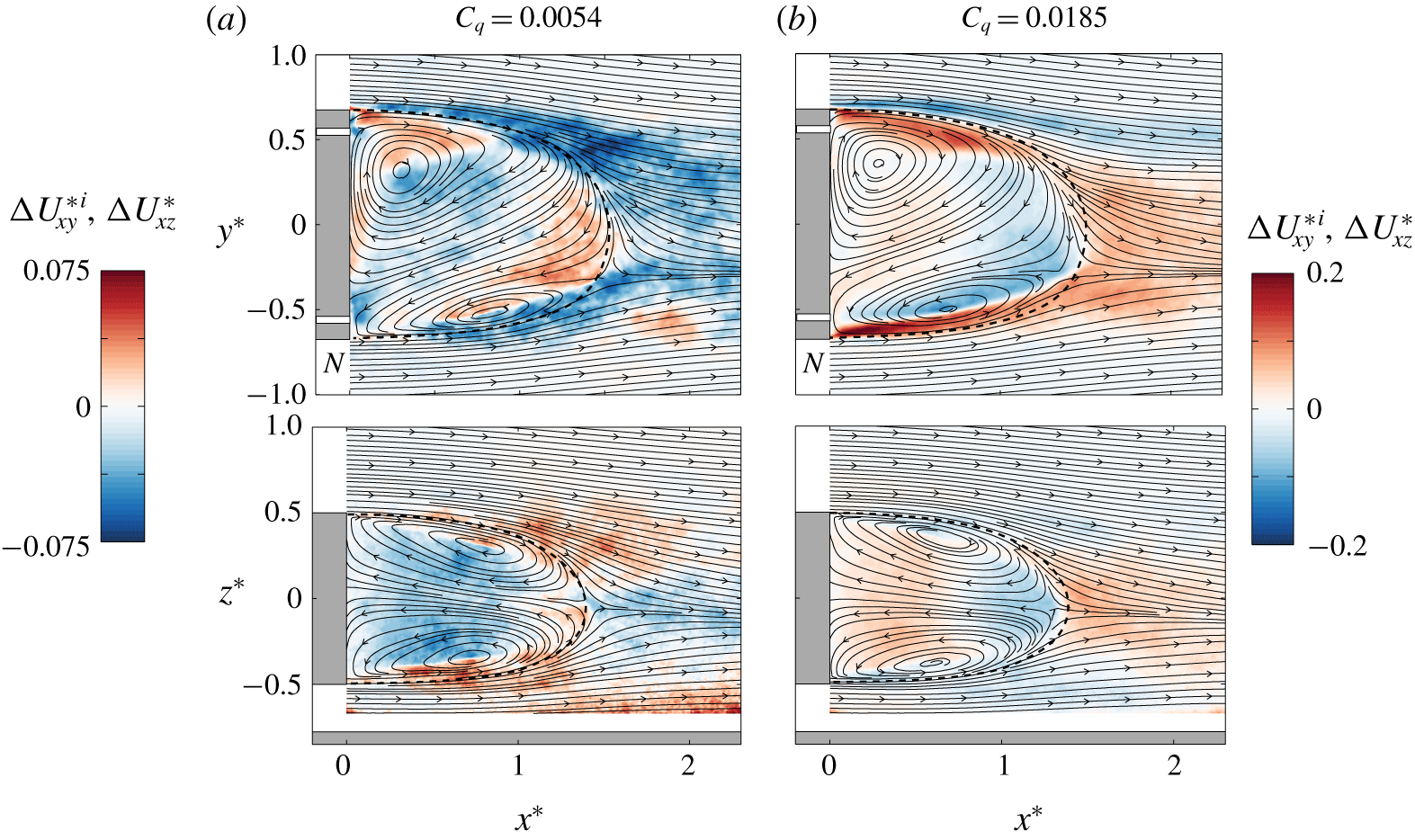
The experimental implementations do not allow for the tracking of the injected mass, but the injected momentum can be assessed by looking at the difference between the mean velocity modulus at a given blowing rate with that of  $C_{q}=0$, say
 $\unicode[STIX]{x0394}U_{xy}^{\ast i}=U_{xy}^{\ast i}-U_{xy0}^{\ast i}$ in the
 $z=0$ plane and
 $\unicode[STIX]{x0394}U_{xz}^{\ast }=U_{xz}^{\ast }-U_{xz0}^{\ast }$ in the
 $y=0$ plane, where
 $i=P$ or
 $N$ denotes the state. Both cases will be referred to as mean momentum modifications. We superimpose on the mean flow streamlines in figure 17 the mean momentum modification when blowing in the LR configuration. We only display the optimal
 $C_{q}^{Opt}$ (figure 17a) and maximal injection
 $C_{q}=0.0185$ (figure 17b) corresponding to the extreme cases of respectively low and high base drag. The blowing jets are not distinguishable in the mass regime (figure 17a, top), but a momentum reduction is clearly visible outside the bubble. This is an indication that the bubble is sweating low momentum by leaking the continuous injection mass. The bubble size is slightly increased when compared to the dashed curve representing the separatrix obtained with no injection. For the maximum injection coefficient in figure 17(b, top), the bubble size is decreased, and the momentum is significantly increased at the exit of the slits inside the bubble. There are also indications of leakage shown by the momentum decrease just outside the bubble at the right-hand side injection and momentum increases after the bubble closure (also observable in the perpendicular plane in figure 17b, bottom). In both cases, it reveals that momentum from the bubble has mixed with the flow outside the bubble and then been naturally transported downstream: at the right outer edge with high-speed flow and in the wake with low-speed flow.
Blowing in LR configuration. Mean momentum modification superimposed on the mean streamlines for (a)  $C_{q}=C_{q}^{Opt}$ and (b) maximum injection
 $C_{q}=0.0185$. (a, top)
 $\unicode[STIX]{x0394}U_{xy}^{\ast i}=U_{xy}^{\ast i}-U_{xy0}^{\ast i}$, (b, bottom)
 $\unicode[STIX]{x0394}U_{xz}^{\ast }=U_{xz}^{\ast }-U_{xz0}^{\ast }$,
 $i=P$ or
 $N$ denotes the state. The dashed curve represents the separatrix of the recirculating bubble with no injection.

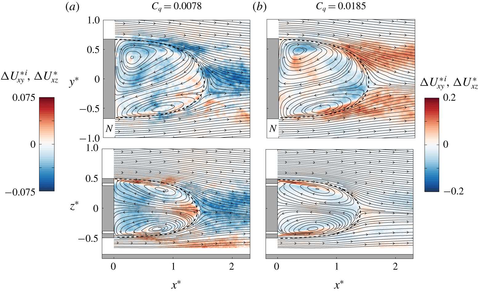
The evacuation of the injected mass by the wake is also observable in figure 18 for the TB configuration. The optimal blowing is associated with an overall momentum reduction outside the bubble in figure 18(a) and the maximal blowing to momentum increase after the bubble in figure 18(b, top). The leakage pattern in the momentum regime is dominant in the plane  $z=0$ and very different from the LR configuration observed in figure 17(b, top). The optimal blowing at
 $C_{q}=0.0078$ also produces a larger bubble size (figure 18a) and the maximal blowing a smaller bubble size (figure 18b).
Similar results are obtained for all other configurations, whose main differences lay only in the leakage pattern of the momentum regime. As a conclusion, the path of the injected flow is never detectable in the mean flow displayed with streamlines as ideally sketched in Bearman (Reference Bearman1967) in the theoretical case of a steady wake but mixed and then evacuated in the wake through the unsteady dynamics of the shear layers and bubble closure.
Blowing in TB configuration. Mean momentum modification superimposed on the mean streamlines for (a)  $C_{q}=C_{q}^{Opt}$ and (b) maximum injection
 $C_{q}=0.0185$. (a, top)
 $\unicode[STIX]{x0394}U_{xy}^{\ast i}=U_{xy}^{\ast i}-U_{xy0}^{\ast i}$, (b, bottom)
 $\unicode[STIX]{x0394}U_{xz}^{\ast }=U_{xz}^{\ast }-U_{xz0}^{\ast }$,
 $i=P$ or
 $N$ denotes the state. The dashed curve represents the separatrix of the recirculating bubble with no injection.

3.6 Drag and recirculation length
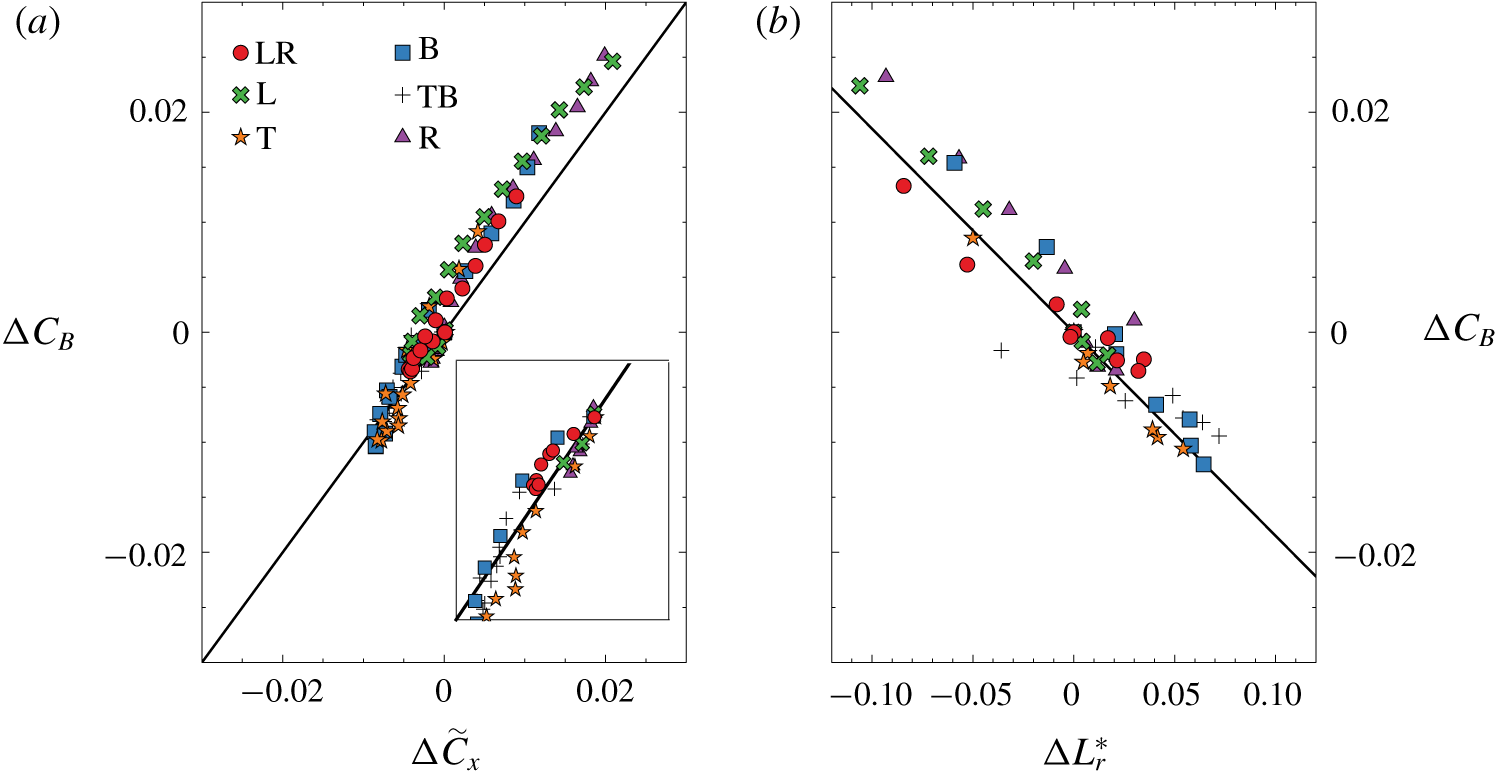
The base drag coefficient variation versus the drag coefficient variation in figure 19(a) deviates slightly from the linear law of slope one. This linear law is expected for a blunt-base geometry when pressure drag is the only source of drag. However, the slope of one is satisfactorily achieved for the mass regime which concerns all the data points from zero to the optimal values of lower drag (figure 19a, inset). A significant curvature is observed when the blowing is further increased above the optimal values (momentum regime) leading to drag increase. This effect is likely to be due to the nonlinear interaction of the blowing jet with the flow at the base, which cannot be assessed in the simple expression of thrust and slit head loss removals as used in (2.6). The plot also points out the good accuracy of the base drag estimation using the four pressure taps, indicating that it is an effective way to access the main characteristics of the base pressure distribution for this geometry.
The bubble recirculating length is correlated to the base drag as can be seen in figure 19(b). The larger the bubble, the smaller the base drag and vice versa. It also indicates that increasing blowing in the mass regime (respectively momentum regime) increases (respectively decreases) the recirculating length. This relationship is illustrated by the results shown in both figures 17 and 18 displaying the shape of the recirculating bubble for lowest (a) and highest (b) base drag of two blowing configurations. The relation between separation length and base drag is a classical result for blunt-base bluff bodies, either two-dimensional (Bearman Reference Bearman1967), axisymmetric (Mariotti, Buresti & Salvetti Reference Mariotti, Buresti and Salvetti2015) or three-dimensional (Grandemange et al. Reference Grandemange, Gohlke and Cadot2013b). The small variations compared to the non-blowing value produce the affine relationship as observed in figure 19(b):
 $$\begin{eqnarray}\displaystyle C_{B}=C_{B0}-0.185(L_{r}^{\ast }-L_{r0}^{\ast }). & & \displaystyle\end{eqnarray}$$
The aim of (3.1) is to highlight the relation between  $C_{B}$ and
 $L_{r}^{\ast }$ when a steady perimetric blowing (of small momentum) is injected through the base of a three-dimensional blunt body. The correlation may depend on the body geometry and flow conditions. Therefore, we cannot ensure that such a dependence is universal, and a different value of the slope and power law may be found in different configurations.
Base drag coefficient versus (a) drag coefficient and (b) recirculating bubble length. The subscript 0 denotes values obtain with  $C_{q}=0$. In (a), the continuous line is
 $\unicode[STIX]{x0394}C_{B}=\unicode[STIX]{x0394}\tilde{C}_{x}$ and the inset is a close-up view of the plot showing data in the mass regime only. In (b), the continuous line is
 $\unicode[STIX]{x0394}C_{B}=-0.185\unicode[STIX]{x0394}L_{r}^{\ast }$.

4 Discussion
4.1 Wake modes sensitivity to local blowing
The sensitivity of the static mode to the local base blowing is summarized in figure 12 for all the asymmetric configurations of blowing and in figure 15 for all the symmetric ones. The static mode strength is weakened by the blowing during the mass regime (empty symbols) with a maximum reduction of  $10\,\%$ to
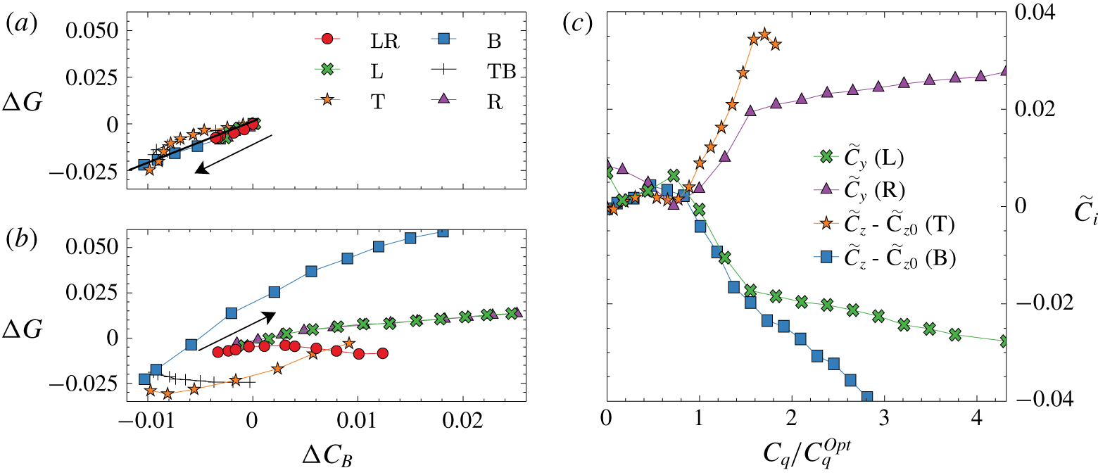
 $20\,\%$ depending on the configuration. Figure 20(a,b) shows the correlation of the base drag variation with the base pressure gradient modulus. Whatever the configuration, there is a well-defined correlation in the mass regime as shown in figure 20(a), indicating that base drag reduction is associated with permanent asymmetry reduction. In the momentum regime, the plot in figure 20(b) is more scattered, with different configurations indicating no straightforward relationship between asymmetry and drag. We can actually distinguish two behaviours. For the LR and TB symmetric configurations for which the wake is always bistable, the base drag is increased, keeping constant the asymmetry strength. For the asymmetric configurations L, R, T and B, the base drag increase is associated with asymmetry strength increase. We believe these effects to be a simple consequence of the symmetry properties of the blowing configuration, where only asymmetric configurations are able to amplify the wake asymmetry.
Static mode orientation, given by the orientation of the base pressure gradient of the state, is found to be sensitive to local blowing. For all asymmetric configurations in the momentum regime, blowing is able to impose the mode orientation, as can be seen in figure 12. While the L or R configuration corresponds to state selection, the T and B configurations force a non-trivial rotation of the static mode. Similar static mode rotation was observed by introducing steady disturbances breaking the top/bottom symmetry of the rectangular base obtained either by small obstructions (Barros et al. Reference Barros, Borée, Cadot, Spohn and Noack2017) or by pitching the body (Bonnavion & Cadot Reference Bonnavion and Cadot2018). The orientation sensitivity of the static mode has a large impact on the aerodynamic force as shown in figure 20. In Bonnavion & Cadot (Reference Bonnavion and Cadot2018) the lateral force produced by the  $P$ and
 $N$ state is shown to be
 $C_{i}=\pm 0.02$ (
 $i=y,z$ denotes the direction of the instability). Thus for
 $C_{q}=1.5C_{q}^{Opt}$ in figure 20(c), the lateral force is mostly produced by the strength of the reoriented static mode rather than by the jet itself.
Variation of base pressure gradient modulus  $\unicode[STIX]{x0394}G=G-G_{0}$ in the (a) mass and (b) momentum regimes versus base drag variation
 $\unicode[STIX]{x0394}C_{B}=C_{B}-C_{B0}$ for all configurations. In both panels the arrows indicate the direction of blowing coefficient
 $C_{q}$ increase. (c) Lateral force coefficients versus the reduced blowing coefficient
 $C_{q}/C_{q}^{Opt}$ for asymmetric slit configurations.

As characterized in Grandemange et al. (Reference Grandemange, Gohlke and Cadot2013a), the spatial envelopes of the low- and high-frequency modes are intimately related to the static mode orientation. Since we do not observe any significant changes in the two frequency values independently to the jet intensity and mode orientation in the analysis presented in figure 16, it is likely that the periodic modes sensitivity is essentially explained by the static mode orientation sensitivity to the blowing.
4.2 Base drag modification
4.2.1 Model
We propose a simple mechanism for the base drag variation aiming at understanding the complexity of figure 7. The starting point is the well-established relationship between the mean bubble recirculation length and base drag for this type of geometry (Grandemange et al. Reference Grandemange, Gohlke and Cadot2013b). The correlation is supported by the inviscid cavity models (Wu Reference Wu1972) that establish a general behaviour of base pressure evolving as positive power laws of the inverse of the cavity length. Physically, the low base pressure is produced by the flow curvature around the cavity. For viscous wake flows at large Reynolds number, this trend still remains, with the recirculating bubble playing the role of the cavity (Roshko Reference Roshko1993). In our case, the variations of the bubble length  $L_{r}$ reported in figure 19(b) are small compared to the reference value of
 $L_{r}^{Ref}=1.45$ that linearizes the power law to the approximation (3.1).
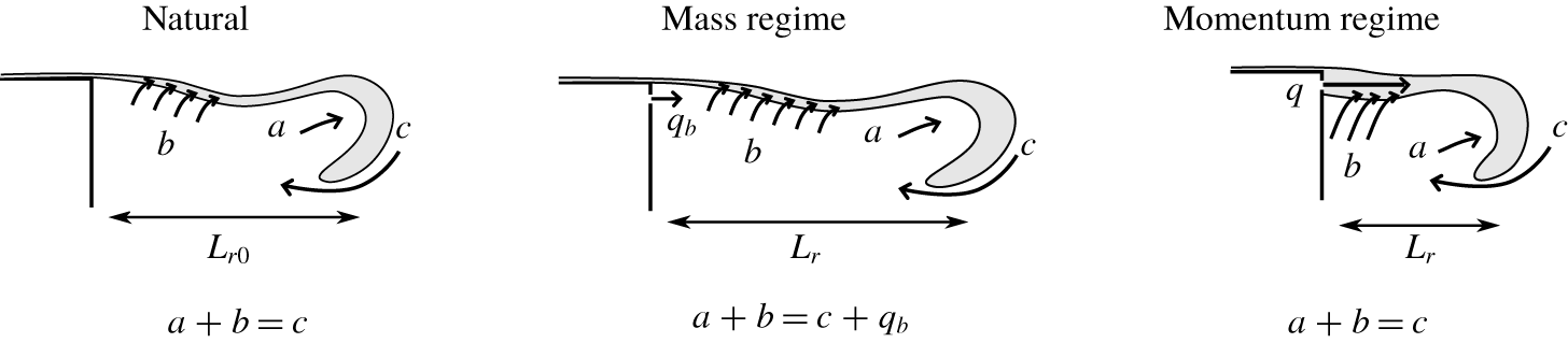
We follow now the mechanism proposed by Gerrard (Reference Gerrard1966) for the adjustment of the recirculating bubble length behind a bluff body. It results from the equilibrium of fluxes filling and emptying the recirculating region. For the natural case, the growth rate of the free shear layers is associated with velocity entrainment along the shear layer, feeding the shear layer by emptying the recirculating region. This total volumetric flux is denoted by  $b$ in figure 21. The key point is that this flux depends on the free shear layer length, and thus increases as
 $L_{r}$ increases and decreases as
 $L_{r}$ decreases. The intense unsteady activity at the bubble closure, such as Kelvin–Helmholtz like instabilities, produces rollups allowing a feedback flux
 $c$ to fill the recirculating region together with a fluid engulfment with flux
 $a$ in the shed vortices (see sketch in figure 21). Momentum of flux
 $c$ is strongly reduced by dissipation. Fluxes
 $a$ and
 $b$ are dominated by the inviscid dynamics of the rollup. The equilibrium of fluxes is
 $a+b=c$. In our case, the mixing layer should be considered as turbulent, known to have a constant growth rate (Champagne, Pao & Wygnanski Reference Champagne, Pao and Wygnanski1976; Pope Reference Pope2000), equivalent to a constant entrainment velocity
 $V_{E}=V_{E}^{\ast }U_{\infty }$ along the shear layers. The flux entrained by the mixing layers delimiting the whole separated region is estimated to
 $b=V_{E}\ell L_{r}$, where
 $\ell$ is the peripheral length of the mixing layers (i.e.
 $\ell =2(h+w)$ for our geometry). The equilibrium for the natural case gives
 $a+V_{E}\ell L_{r0}=c$, where
 $L_{r0}$ is the natural bubble length (i.e. without blowing).
Conceptual sketch illustrating the flow rate budget between filling and emptying of the separated region (see text) for the natural wake, low flow rate injection (mass regime) and large flow rate injection (momentum regime). Grey contours depict the free shear layer that develops from the separation. At a further stage of the unsteady dynamics, the shear layer rollup produces a detached vortex that evacuates downstream fluxes  $b$ and
 $a$ from the separated region.

The mass regime is characterized by an external flux that feeds the recirculating region but whose momentum is dissipated. Compared to the natural scenario described above, we only need to take into account the additional flow rate source  $q=q_{b}$ to
 $c$. The mass regime equilibrium illustrated in figure 21 leads to
 $a+V_{E}\ell L_{r}=c+q_{b}$. As momentum of flux
 $q_{b}$ is dissipated, we should not expect any significant modifications of the flow, and so for fluxes
 $a$ and
 $c$ from the natural case. Hence the flow rate budget gives
 $$\begin{eqnarray}\displaystyle L_{r}=L_{r0}+\frac{q_{b}}{V_{E}\ell }. & & \displaystyle\end{eqnarray}$$
For this mass regime, the recirculation length increases as the injection flux  $q_{b}$ increases with a slope depending on the mean entrainment velocity of the extended shear layer length. This can be pictured as the inflation of the recirculating bubble by the base blowing flux, thus increasing shear layer length and flux leaking through the shear layers, until these two fluxes compensate. The leaking is evidenced with the observation of low-momentum sweating in the results in § 3.5.
On the other hand, the momentum regime is characterized by a deflating of the recirculating bubble with a reduction of the recirculating length as base blowing is increased (see § 3.6). In contrast to the mass regime, the momentum of the blowing flux strongly modifies the flow by entirely evacuating the flux  $q_{b}$ through the shear together with increasing the shear layer entrainment velocity. This modification would be responsible for emptying the recirculating region, i.e. no injection in the recirculating region,
 $q=0$ and increase of flux
 $b$ that would readjust the bubble length (see the sketch of the momentum regime in figure 21). To retrieve the observed effect, the flux entrained by the shear layers must be a combination of disturbed and undisturbed free shear layers,
 $b=(\unicode[STIX]{x1D6FC}_{1}U_{\infty }+\unicode[STIX]{x1D6FC}_{2}U_{b})\ell L_{r}$, and the contributions of
 $a$ and
 $c$ are constant. The flow rate budget
 $a+(\unicode[STIX]{x1D6FC}_{1}U_{\infty }+\unicode[STIX]{x1D6FC}_{2}U_{b})\ell L_{r}=c$ leads to
 $$\begin{eqnarray}\displaystyle L_{r}=\frac{L_{r1}}{1+{\displaystyle \frac{\unicode[STIX]{x1D6FC}_{2}}{\unicode[STIX]{x1D6FC}_{1}}}{\displaystyle \frac{U_{b}}{U_{\infty }}}}\approx L_{r1}\left(1-\frac{\unicode[STIX]{x1D6FC}_{2}}{\unicode[STIX]{x1D6FC}_{1}}\frac{U_{b}}{U_{\infty }}\right). & & \displaystyle\end{eqnarray}$$
Non-dimensional expressions for (4.1) and (4.2) are
 $$\begin{eqnarray}\displaystyle L_{r}^{\ast }=L_{r0}^{\ast }+\frac{w}{V_{E}^{\ast }\ell }C_{q},\quad L_{r}^{\ast }=L_{r1}^{\ast }\left(1-\frac{\unicode[STIX]{x1D6FC}_{2}}{\unicode[STIX]{x1D6FC}_{1}}C_{u}\right). & & \displaystyle\end{eqnarray}$$
4.2.2 Mass regime
The values of  $V_{E}^{\ast }$ displayed in table 4 are computed from (4.3) using the correlation (3.1) providing
 $\unicode[STIX]{x2202}C_{B}/\unicode[STIX]{x2202}C_{q}=-0.185L_{r}^{\ast }$ and the measured slope
 $(\unicode[STIX]{x2202}C_{B}/\unicode[STIX]{x2202}C_{q})|_{0}$ in table 3:
 $$\begin{eqnarray}\displaystyle V_{E}^{\ast }=-0.185\frac{w}{\left.{\displaystyle \frac{\unicode[STIX]{x2202}C_{B}}{\unicode[STIX]{x2202}C_{q}}}\right|_{0}\ell }. & & \displaystyle\end{eqnarray}$$
Classical measurements in mixing layers (Champagne et al. Reference Champagne, Pao and Wygnanski1976; Dimotakis Reference Dimotakis1991; Pope Reference Pope2000) report the parameter  $S$, defined as
 $S=(U_{C}/U_{S})\,\text{d}\unicode[STIX]{x1D6FF}/\text{d}x$, where
 $U_{C}$ is the mean shear velocity,
 $U_{S}$ the velocity jump and
 $\text{d}\unicode[STIX]{x1D6FF}/\text{d}x$ the growth rate of the mixing layer. In our case
 $U_{S}=U_{\infty }$ for which a simple flow rate budget gives
 $V_{E}\,\text{d}x=U_{C}\,\text{d}\unicode[STIX]{x1D6FF}$, thus
 $S=V_{E}^{\ast }$. The range of reported values is from
 $S\approx 0.06$ to
 $S\approx 0.11$ for undisturbed mixing layers (Dimotakis Reference Dimotakis1991). This wide range is related to high sensitivities to the initial condition of the mixing layer at separation. The values we obtained for
 $V_{E}^{\ast }$ in table 4 match satisfactorily this range, indicating that the budget volumetric model is plausible to explain the drag reduction in the mass regime. The assumption that injected momentum does not modify the flow dynamics in the mass regime implies an independence of the bubble growth with the blowing location. It is actually almost the case for the L, R and LR configurations for which the
 $V_{E}^{\ast }$ values are in the range
 $0.059{-}0.075$. It is even better shown by the identical slopes in figure 9(b) whether injection occurs in the adverse flow region (figure 9d, top) or reversed flow region (figure 9d, bottom) of the separated bubble. For these three configurations, the flow characteristics given in table 1 are almost identical. This is not the case for the T and B configurations, indicating significant changes in the vertical base pressure gradient component. Hence, one can argue that the free shear properties, and thus the
 $V_{E}^{\ast }$ values, can change from one configuration to the other due to the influence of the slit on the initial condition of the free shear layer development.

4.2.3 Momentum regime
The ratio  $\unicode[STIX]{x1D6FC}_{2}/\unicode[STIX]{x1D6FC}_{1}$ can also be estimated using again the correlation (3.1) in (4.3), providing
 $$\begin{eqnarray}\displaystyle C_{B}-C_{B0}=-0.185(L_{r1}^{\ast }-L_{r0}^{\ast })+0.185L_{r1}^{\ast }\frac{\unicode[STIX]{x1D6FC}_{2}}{\unicode[STIX]{x1D6FC}_{1}}C_{u}, & & \displaystyle\end{eqnarray}$$
and the linear regression obtained in the momentum regime displayed in table 3. Values for  $\unicode[STIX]{x1D6FC}_{2}/\unicode[STIX]{x1D6FC}_{1}$ are displayed in table 4. The ratio is a measurement of the efficiency of the perturbed shear layers by the momentum injection to evacuate fluid from the recirculating region. We can see in table 4 a wide variation of the ratio, and the basic expectation of having twice the value of the single slit configurations for the double slit configurations is not at all respected.
The smallest value of  $\unicode[STIX]{x1D6FC}_{2}/\unicode[STIX]{x1D6FC}_{1}$ is obtained for the L or R blowing, for which the corresponding forced flow is shown in figure 8(c). The largest ratio is obtained in either the T or B configuration, for which the forced flow is shown in figure 11(c). For all of these single slit configurations, the jet is blowing in an adverse flow region of the static mode, at the outer edge of the steady vortex. The main difference between the lateral and top/bottom blowing is that the global rotation of the static mode has inverted the base aspect ratio of the recirculating region. It is likely that the difference in the wake base aspect ratio is the cause for the discrepancies in the shear ratio values
 $\unicode[STIX]{x1D6FC}_{2}/\unicode[STIX]{x1D6FC}_{1}$.
Intermediate values are found for the symmetric configurations for which bistability persists, and where the static mode still remains oriented in the horizontal direction (figure 14a). For the case of the TB configuration, the blowing is never located at the outer edge of the steady vortex as for the single T injection (figure 11c), but in the highly fluctuating shear layers as shown in figure 14(c), likely to be much less efficient in evacuating fluid from the recirculation region. For the LR configuration (figure 13c), there is one blowing slit located at the outer edge of the steady vortex as for the single L or R injection (figure 8c), while the other slit blows in the reversed flow region in the proximity of a highly fluctuating shear layer. This permanent asymmetry plausibly explains why the value of  $\unicode[STIX]{x1D6FC}_{2}/\unicode[STIX]{x1D6FC}_{1}$ for the LR configuration is lower than twice that of the L or R configuration.
4.3 Critical blowing of the transition
If the transition defined by the minimum base drag value is determined by a critical parameter associated with each slit, we would expect the critical parameter for the TB configuration to be the mean of the critical parameters obtained for T and B transition. This is not true if the parameter is the momentum coefficient  $C_{u}$, as can be seen in figure 7(b). It is then unlikely that the momentum coefficient
 $C_{u}$ could be the critical parameter for the transition between the mass and the momentum regimes. However, by looking at the
 $C_{q}$ plot in figure 7(a), the transition value for the TB configuration
 $C_{q}^{Opt}=7.8\times 10^{-3}$ is between the two transition values
 $C_{q}^{Opt}=10.2\times 10^{-3}$ of the T configuration and
 $C_{q}^{Opt}=6.6\times 10^{-3}$ of the B configuration and matches approximately the average value. For the LR configuration, the flow is always bistable, which means that, during the random switching dynamics between the
 $P$ and
 $N$ state, one slit is permanently injecting in the adverse flow region while the other is permanently injecting in the reversed flow region (see figure 13). For consistency with the T, B and TB configurations discussed above, we would expect that the LR transition value should match the average of the transition values for a single injection in the reversed flow region and a single injection in the adverse flow region. These two transition values are given for the wake either locked in a
 $P$ state or an
 $N$ state with a single slit injection. This is exactly the case studied in figure 9 in the R blowing configuration. The transition for the
 $N$ state occurs at
 $C_{q}^{Opt}=4.3\times 10^{-3}$ while for the
 $P$ state
 $C_{q}^{Opt}=6.6\times 10^{-3}$. The transition value
 $C_{q}^{Opt}=5.5\times 10^{-3}$ of the LR configuration is then also between the two single cases and approximately corresponds to their average. This consistency between the configurations in the
 $C_{q}$ plot and the discrepancy in the
 $C_{u}$ plot shows that the transition between the mass and the momentum regimes is governed by a critical value of the global injected flow rate (also depending on the location of the injection) and not the mean momentum of the base blowing. It seems contradictory to the results of Wood (Reference Wood1964) and may emphasize differences whether the flow is two-dimensional with injection in the middle of the base (Wood Reference Wood1964) or three-dimensional with injections at the proximity of the shear layers (the present study).
Finally, to extend the mass regime and then to increase the base drag reduction, it is favourable to inject in a reversed flow region of the recirculating bubble (see figures 9 and 10). It is likely that the injected jet momentum dissipation is enhanced in this case.
5 Conclusions
It is known that, in two-dimensional bodies, a bleed has a stabilizing effect on the global instability, and von Kármán vortex shedding can be substantially weakened, resulting in a large drag reduction. However, in the three-dimensional bluff bodies of interest in the present work, shear instabilities are still present but their contribution to drag is weaker and the resulting effects of bleed on the near-wake flow are mainly related to the manipulation and control of the static modes.
In particular, there are two very distinctive sensitivities of three-dimensional wake modes to local base blowing whether blowing is in the mass or momentum regime. The mass regime shows almost no dependence on the injection location; it is accompanied by the recirculating bubble inflating, producing the drag reduction. In addition to these observations, which are common to two-dimensional bluff bodies, it is found in this work that the mass regime is characterized by a reduction of the static asymmetric mode strength. The flow makes a transition to the momentum regime for a critical flow rate depending on the injection location. The momentum regime is found to be mainly governed by the interaction with the static asymmetric mode, either selecting a pre-existing state or forcing a rotation of the static mode orientation. This interaction leads to drastic changes of the recirculating bubble topology, while the periodic mode shapes are found to follow the modification of the static mode orientation. Compared to two-dimensional bluff bodies, the interaction leads to non-trivial base drag variation with blowing location and intensity. There is no straightforward correlation with the static mode strength, but, globally, the momentum regime is associated with a recirculating bubble deflating together with a drag increase. The experimental results are used to build a flow rate budget model of the recirculating region taking into account shear layer modification for the momentum regime. The work offers an experimental database with comprehensive interaction of base blowing with the three-dimensional wake and its main modes. It could be used in the future for flow control in the presence of a static asymmetric wake mode.
Acknowledgements
The authors are grateful to P. Bearman for useful discussions and the critical reading of the manuscript. This work has been partially supported by the Spanish MINECO and European Funds under projects DPI2017-89746-R and DPI2017-88201-C3-2-R. Moreover, J.I.J.-G. and M.L.-D. want to thank the Spanish MECD for the financial support provided under José Castillejo grant CAS18/00379 and Fellowship FPU 014/02945, respectively.
Declaration of interests
The authors report no conflict of interest.