2.1. The dimensionless free-surface Euler equations

We non-dimensionalize the equations by using several lengths: the typical amplitude $a_{surf}$ of the waves, the typical amplitude $a_{bott}$ of the bottom variations, the typical depth $H_{0}$ and the typical horizontal scale $L$ . Using these quantities, it is possible to form three dimensionless parameters,

(2.1a−c ) $$\begin{eqnarray}{\it\varepsilon}=\frac{a_{surf}}{H_{0}},\quad {\it\beta}=\frac{a_{bott}}{H_{0}},\quad {\it\mu}=\frac{H_{0}^{2}}{L^{2}};\end{eqnarray}$$

the parameters ${\it\varepsilon}$ and ${\it\beta}$ are often called nonlinearity (or amplitude) and topography parameters, and the parameter ${\it\mu}$ is the shallowness parameter.

We also use $a_{surf}$ , $a_{bott}$ , $H_{0}$ and $L$ to define dimensionless variables and unknowns (written with a tilde),

(2.2a−d ) $$\begin{eqnarray}\tilde{z}=\frac{z}{H_{0}},\quad \tilde{X}=\frac{X}{L},\quad \tilde{{\it\zeta}}=\frac{{\it\zeta}}{a_{surf}},\quad \tilde{b}=\frac{b}{a_{bott}};\end{eqnarray}$$

the non-dimensionalization of the time variable and of the velocity and pressure fields is based on the linear analysis of the equations (see for instance Lannes (Reference Lannes2013, Chap. 1))

(2.3a−d ) $$\begin{eqnarray}\tilde{\boldsymbol{V}}=\frac{\boldsymbol{V}}{V_{0}},\quad \tilde{\boldsymbol{w}}=\frac{\boldsymbol{w}}{w_{0}},\quad \tilde{t}=\frac{t}{t_{0}},\quad \tilde{P}=\frac{P}{P_{0}},\end{eqnarray}$$

with

(2.4a−d ) $$\begin{eqnarray}V_{0}=a\sqrt{\frac{g}{H_{0}}},\quad w_{0}=\frac{aL}{H_{0}}\sqrt{\frac{g}{H_{0}}},\quad t_{0}=\frac{L}{\sqrt{gH_{0}}},\quad P_{0}={\it\rho}gH_{0}.\end{eqnarray}$$

With these variables and unknowns, and with the notations

(2.5a−c ) $$\begin{eqnarray}\boldsymbol{U}^{{\it\mu}}=\left(\begin{array}{@{}c@{}}\sqrt{{\it\mu}}\boldsymbol{V}\\ \boldsymbol{ w }\end{array}\right),\quad \boldsymbol{{\rm\nabla}}^{{\it\mu}}=\left(\begin{array}{@{}c@{}}\sqrt{{\it\mu}}\boldsymbol{{\rm\nabla}}\\ \partial _{z}\end{array}\right),\quad N^{{\it\mu}}=\left(\begin{array}{@{}c@{}}-{\it\varepsilon}\sqrt{{\it\mu}}\boldsymbol{{\rm\nabla}}{\it\zeta}\\ 1\end{array}\right),\end{eqnarray}$$

and

(2.6a−c ) $$\begin{eqnarray}\text{curl}^{{\it\mu}}=\boldsymbol{{\rm\nabla}}^{{\it\mu}}\times ,\quad \text{div}^{{\it\mu}}=(\boldsymbol{{\rm\nabla}}^{{\it\mu}})^{\text{T}},\quad \underline{U}^{{\it\mu}}=(\sqrt{{\it\mu}}\underline{V}^{\text{T}},\underline{w})^{\text{T}}:=\boldsymbol{U}_{|_{z={\it\varepsilon}{\it\zeta}}}^{{\it\mu}},\end{eqnarray}$$

the incompressible Euler equations take the form (omitting the tildes)

(2.7) $$\begin{eqnarray}\displaystyle \partial _{t}\boldsymbol{U}^{{\it\mu}}+\frac{{\it\varepsilon}}{{\it\mu}}\boldsymbol{U}^{{\it\mu}}\boldsymbol{\cdot }\boldsymbol{{\rm\nabla}}^{{\it\mu}}\boldsymbol{U}^{{\it\mu}} & = & \displaystyle -\frac{1}{{\it\varepsilon}}(\boldsymbol{{\rm\nabla}}^{{\it\mu}}P+\boldsymbol{e}_{z})\quad \text{in}\ {\it\Omega}_{t},\end{eqnarray}$$

(2.8) $$\begin{eqnarray}\displaystyle \text{div}^{{\it\mu}}\boldsymbol{U}^{{\it\mu}} & = & \displaystyle 0\quad \text{in}\ {\it\Omega}_{t},\end{eqnarray}$$

${\it\Omega}_{t}$

(2.9) $$\begin{eqnarray}{\it\Omega}_{t}=\{(X,z)\in \mathbb{R}^{d+1},-1+{\it\beta}b(X)<z<{\it\varepsilon}{\it\zeta}(t,X)\}.\end{eqnarray}$$

Finally, the boundary conditions on the velocity read in dimensionless form

(2.10) $$\begin{eqnarray}\displaystyle & \partial _{t}{\it\zeta}+\boldsymbol{{\rm\nabla}}\boldsymbol{\cdot }(h\overline{V})=0\quad \text{at the surface}, & \displaystyle\end{eqnarray}$$

(2.11) $$\begin{eqnarray}\displaystyle & P=0\quad \text{at the surface}, & \displaystyle\end{eqnarray}$$

(2.12) $$\begin{eqnarray}\displaystyle & \boldsymbol{U}_{|_{z=-1+{\it\beta}b}}^{{\it\mu}}\boldsymbol{\cdot }N_{b}^{{\it\mu}}=0\quad \text{at the bottom}, & \displaystyle\end{eqnarray}$$

$N_{b}^{{\it\mu}}=(-{\it\varepsilon}\sqrt{{\it\mu}}\boldsymbol{{\rm\nabla}}b^{\text{T}},1)^{\text{T}}$

$h$

$\overline{V}$

(2.13a,b ) $$\begin{eqnarray}h(t,X):=1+{\it\varepsilon}{\it\zeta}(t,X)-{\it\beta}b(X),\quad \overline{V}(t,X)=\frac{1}{h}\int _{-1+{\it\beta}b(X)}^{{\it\varepsilon}{\it\zeta}(t,X)}\boldsymbol{V}(t,X,z)\text{d}z.\end{eqnarray}$$

Decomposing the horizontal velocity into

(2.14) $$\begin{eqnarray}\boldsymbol{V}(t,X,z)=\overline{V}(t,X)+\sqrt{{\it\mu}}V^{\ast }(t,X,z),\end{eqnarray}$$

the dimensionless version of (1.11) is then given by

(2.15) $$\begin{eqnarray}\left.\begin{array}{@{}c@{}}\partial _{t}{\it\zeta}+\boldsymbol{{\rm\nabla}}\boldsymbol{\cdot }(h\overline{V})=0,\\ \displaystyle \partial _{t}(h\overline{V})+{\it\varepsilon}\boldsymbol{{\rm\nabla}}\boldsymbol{\cdot }(h\overline{V}\otimes \overline{V})+{\it\varepsilon}{\it\mu}\boldsymbol{{\rm\nabla}}\boldsymbol{\cdot }\left(\int _{-1+{\it\beta}b}^{{\it\varepsilon}{\it\zeta}}V^{\ast }\otimes V^{\ast }\right)+\frac{1}{{\it\varepsilon}}\int _{-1+{\it\beta}b}^{{\it\varepsilon}{\it\zeta}}\boldsymbol{{\rm\nabla}}P=0.\end{array}\right\}\end{eqnarray}$$

We therefore need to express the ‘rotational Reynolds tensor’ $\int _{-1+{\it\beta}b}^{{\it\varepsilon}{\it\zeta}}V^{\ast }\otimes V^{\ast }$ and the pressure contribution $(1/{\it\varepsilon})\int _{-1+{\it\beta}b}^{{\it\varepsilon}{\it\zeta}}\boldsymbol{{\rm\nabla}}P$ in terms of ${\it\zeta}$ and $\overline{V}$ in order to obtain a closed set of equations. This requires a good understanding of the behaviour of the vorticity ${\bf\omega}_{{\it\mu}}$ , defined as

(2.16) $$\begin{eqnarray}{\bf\omega}_{{\it\mu}}=\left(\begin{array}{@{}c@{}}\displaystyle \frac{1}{\sqrt{{\it\mu}}}(\partial _{z}\boldsymbol{V}^{\bot }-\boldsymbol{{\rm\nabla}}^{\bot }\boldsymbol{w})\\ \displaystyle -\boldsymbol{{\rm\nabla}}\boldsymbol{\cdot }\boldsymbol{V}^{\bot }\end{array}\right)=\frac{1}{{\it\mu}}\;\text{curl}^{{\it\mu}}\boldsymbol{U}^{{\it\mu}}.\end{eqnarray}$$

We shall assume here that ${\bf\omega}_{{\it\mu}}$ is of order $O(1)$ with respect to ${\it\mu}$ (in the terminology of Teshukov (Reference Teshukov2007) and Richard & Gavrilyuk (Reference Richard and Gavrilyuk2012), we consider therefore weakly sheared flows). It is rigorously shown in Castro & Lannes (Reference Castro and Lannes2014) that in this regime, ${\it\zeta}$ , $\overline{V}$ and ${\bf\omega}_{{\it\mu}}$ remain $O(1)$ quantities during the time evolution of the flow. All the formal asymptotic descriptions made throughout this article therefore have a firm basis, and the models derived here could be rigorously justified using the procedure hinted at in Castro & Lannes (Reference Castro and Lannes2014) (and carried through for the Saint-Venant equations with vorticity).

2.2. Asymptotic expansion of the velocity field

As explained above, the quantities ${\it\zeta}$ , $\overline{V}$ and ${\bf\omega}_{{\it\mu}}$ are all of order $O(1)$ with respect to ${\it\mu}$ . An asymptotic description of $\boldsymbol{U}^{{\it\mu}}$ can then be found by considering the boundary value problem

(2.17) $$\begin{eqnarray}\left.\begin{array}{@{}lc@{}}\text{curl}^{{\it\mu}}\boldsymbol{U}^{{\it\mu}}={\it\mu}{\bf\omega}_{{\it\mu}} & \text{in}\ {\it\Omega}\\ \text{div}^{{\it\mu}}\boldsymbol{U}^{{\it\mu}}=0 & \text{in}\ {\it\Omega}\\ U_{b}^{{\it\mu}}\boldsymbol{\cdot }N_{b}^{{\it\mu}}=0 & \text{at the bottom}\end{array}\right\}\end{eqnarray}$$

(the subscript $b$ is used to denote quantities evaluated at the bottom).

Remark 3. Only the ‘rotational’ part of $\boldsymbol{U}^{{\it\mu}}$ is fully determined from this boundary value problem. The ‘irrotational part’ of $\boldsymbol{U}^{{\it\mu}}$ is determined from the tangential component of the velocity at the interface; more precisely, one can show that $\boldsymbol{U}_{\Vert }^{{\it\mu}}:=\boldsymbol{V}_{|_{z={\it\varepsilon}{\it\zeta}}}+{\it\varepsilon}\boldsymbol{w}_{|_{z={\it\varepsilon}{\it\zeta}}}\boldsymbol{{\rm\nabla}}{\it\zeta}$ can be written under the form

(2.18) $$\begin{eqnarray}\boldsymbol{U}_{\Vert }^{{\it\mu}}=\boldsymbol{{\rm\nabla}}{\it\psi}+\boldsymbol{{\rm\nabla}}^{\bot }{\it\Delta}^{-1}({{\bf\omega}_{{\it\mu}}}_{|_{z={\it\varepsilon}{\it\zeta}}}\boldsymbol{\cdot }N^{{\it\mu}}),\end{eqnarray}$$

for some scalar function ${\it\psi}$ defined over $\mathbb{R}^{2}$ . This function fully determines the ‘irrotational’ part of $\boldsymbol{U}^{{\it\mu}}$ , which is given by $\boldsymbol{{\rm\nabla}}^{{\it\mu}}{\it\Phi}$ , with

(2.19) $$\begin{eqnarray}\left.\begin{array}{@{}l@{}}(\partial _{z}^{2}+{\it\mu}{\it\Delta}){\it\Phi}=0\quad \text{in}\ {\it\Omega}\\ {\it\Phi}_{|_{surf}}={\it\psi},\quad \partial _{z}{\it\Phi}_{|_{bott}}=0\end{array}\right\}\end{eqnarray}$$

(and which obviously leaves (2.17) unchanged). We refer to Castro & Lannes (Reference Castro and Lannes2014) for more details; it is, in particular, shown in this reference that ${\it\zeta}$ , ${\it\psi}$ and ${\bf\omega}_{{\it\mu}}$ remain uniformly bounded with respect to ${\it\mu}$ during the time evolution of the flow. The analysis of the full boundary value problem then shows that $\boldsymbol{V}$ , $\boldsymbol{ w}$ , $\overline{V}$ etc. also remain bounded, which justifies the formal asymptotics made here.

We show here how to construct an approximate solution to this system of equations. Replacing

(2.20) $$\begin{eqnarray}\boldsymbol{U}^{{\it\mu}}=\left(\begin{array}{@{}c@{}}\sqrt{{\it\mu}}\boldsymbol{V}\\ \boldsymbol{ w }\end{array}\right)=\left(\begin{array}{@{}c@{}}\sqrt{{\it\mu}}\overline{V}+{\it\mu}V^{\ast }\\ {\it\mu}\tilde{\boldsymbol{w}}\end{array}\right)\end{eqnarray}$$

in (2.17) and using the fact that $\partial _{z}\overline{V}=0$ , we obtain

(2.21) $$\begin{eqnarray}\left.\begin{array}{@{}l@{}}\partial _{z}V^{\ast }-\sqrt{{\it\mu}}\boldsymbol{{\rm\nabla}}\tilde{\boldsymbol{w}}=-{\bf\omega}_{{\it\mu},h}^{\bot }\quad \text{in}\ {\it\Omega}\\ \boldsymbol{{\rm\nabla}}^{\bot }\boldsymbol{\cdot }\overline{V}+\sqrt{{\it\mu}}\boldsymbol{{\rm\nabla}}^{\bot }\boldsymbol{\cdot }V^{\ast }={\bf\omega}_{{\it\mu},v}\quad \text{in}\ {\it\Omega}\\ \boldsymbol{{\rm\nabla}}\boldsymbol{\cdot }\overline{V}+\sqrt{{\it\mu}}\boldsymbol{{\rm\nabla}}\boldsymbol{\cdot }V^{\ast }+\partial _{z}\tilde{\boldsymbol{w}}=0\quad \text{in}\ {\it\Omega}\\ \tilde{\boldsymbol{w}}_{b}-{\it\beta}\boldsymbol{{\rm\nabla}}b\boldsymbol{\cdot }(\overline{V}+\sqrt{{\it\mu}}V_{b}^{\ast })=0\quad \text{at the bottom},\end{array}\right\}\end{eqnarray}$$

where ${\bf\omega}_{{\it\mu},h}$ and ${\bf\omega}_{{\it\mu},v}$ denote respectively the horizontal and vertical components of the vorticity ${\bf\omega}_{{\it\mu}}$ . From the third and last equations of (2.21), we first get an expression for $\tilde{\boldsymbol{w}}$ in terms of $\overline{V}$ and $V^{\ast }$ ,

(2.22) $$\begin{eqnarray}\tilde{\boldsymbol{w}}=-\boldsymbol{{\rm\nabla}}\boldsymbol{\cdot }[(1+z-{\it\beta}b)\overline{V}]-\sqrt{{\it\mu}}\boldsymbol{{\rm\nabla}}\boldsymbol{\cdot }\int _{-1+{\it\beta}b}^{z}V^{\ast }.\end{eqnarray}$$

Replacing this expression in the first equation of (2.21) then gives

(2.23) $$\begin{eqnarray}\partial _{z}V^{\ast }=\sqrt{{\it\mu}}\boldsymbol{{\rm\nabla}}\tilde{\boldsymbol{w}}-{\bf\omega}_{{\it\mu},h}^{\bot }\end{eqnarray}$$

and therefore

(2.24) $$\begin{eqnarray}V^{\ast }=\sqrt{{\it\mu}}\left(\int _{z}^{{\it\varepsilon}{\it\zeta}}\boldsymbol{{\rm\nabla}}\boldsymbol{{\rm\nabla}}\boldsymbol{\cdot }[(1+z^{\prime }-{\it\beta}b)\overline{V}]\text{d}z^{\prime }\!\right)^{\!\ast }+{\it\mu}\left(\int _{z}^{{\it\varepsilon}{\it\zeta}}\boldsymbol{{\rm\nabla}}\boldsymbol{{\rm\nabla}}\boldsymbol{\cdot }\int _{-1+{\it\beta}b}^{z}V^{\ast }\!\!\right)^{\ast }+\left(\int _{z}^{{\it\varepsilon}{\it\zeta}}{\bf\omega}_{{\it\mu},h}^{\bot }\!\right)^{\ast }.\end{eqnarray}$$

Defining the operators $T=T[{\it\beta}b,{\it\varepsilon}{\it\zeta}]$ and $T^{\ast }=T^{\ast }[{\it\beta}b,{\it\varepsilon}{\it\zeta}]$ by

(2.25a,b ) $$\begin{eqnarray}T[{\it\beta}b,{\it\varepsilon}{\it\zeta}]W=\int _{z}^{{\it\varepsilon}{\it\zeta}}\boldsymbol{{\rm\nabla}}\boldsymbol{{\rm\nabla}}\boldsymbol{\cdot }\int _{-1+{\it\beta}b}^{z^{\prime }}W\quad \text{and}\quad T^{\ast }[{\it\beta}b,{\it\varepsilon}{\it\zeta}]W=(T[{\it\beta}b,{\it\varepsilon}{\it\zeta}]W)^{\ast },\end{eqnarray}$$

and the ‘shear’ velocity $V_{sh}$ by

(2.26) $$\begin{eqnarray}V_{sh}=\int _{z}^{{\it\varepsilon}{\it\zeta}}{\bf\omega}_{{\it\mu},h}^{\bot },\end{eqnarray}$$

we can rewrite the above identity under the form

(2.27) $$\begin{eqnarray}(1-{\it\mu}T^{\ast })V^{\ast }=\sqrt{{\it\mu}}T^{\ast }\overline{V}+V_{sh}^{\ast }.\end{eqnarray}$$

It should be noted that this is an exact identity. Applying $(1+{\it\mu}T^{\ast })$ on both sides, we obtain the following approximation of order $O({\it\mu}^{3/2})$ :

(2.28) $$\begin{eqnarray}V^{\ast }=\sqrt{{\it\mu}}T^{\ast }\overline{V}+(1+{\it\mu}T^{\ast })V_{sh}^{\ast }+O({\it\mu}^{3/2}).\end{eqnarray}$$

Together with (2.14), this yields the following $O({\it\mu})$ and $O({\it\mu}^{2})$ approximations for the horizontal velocity field $\boldsymbol{V}$ :

(2.29) $$\begin{eqnarray}\displaystyle & \boldsymbol{V}=\overline{V}+\sqrt{{\it\mu}}V_{sh}^{\ast }+O({\it\mu}), & \displaystyle\end{eqnarray}$$

(2.30) $$\begin{eqnarray}\displaystyle & \boldsymbol{V}=\overline{V}+\sqrt{{\it\mu}}V_{sh}^{\ast }+{\it\mu}T^{\ast }\overline{V}+{\it\mu}^{3/2}T^{\ast }V_{sh}^{\ast }+O({\it\mu}^{2}). & \displaystyle\end{eqnarray}$$

Remark 5. Since $\overline{V}$ does not depend on $z$ , one can compute explicitly

(2.31) $$\begin{eqnarray}T^{\ast }\overline{V}=-\frac{1}{2}\left((z+1-{\it\beta}b)^{2}-\frac{h^{2}}{3}\right)\boldsymbol{{\rm\nabla}}\boldsymbol{{\rm\nabla}}\boldsymbol{\cdot }\overline{V}+{\it\beta}\left(z-{\it\varepsilon}{\it\zeta}+\frac{1}{2}h\right)[\boldsymbol{{\rm\nabla}}b\boldsymbol{\cdot }\boldsymbol{{\rm\nabla}}\overline{V}+\boldsymbol{{\rm\nabla}}(\boldsymbol{{\rm\nabla}}b\boldsymbol{\cdot }\overline{V})].\end{eqnarray}$$

Finally, for the vertical component $\boldsymbol{w}$ of the velocity, we use (2.28) together with (2.20) and (2.22) to obtain

(2.32) $$\begin{eqnarray}\displaystyle & \boldsymbol{w}=O({\it\mu}), & \displaystyle\end{eqnarray}$$

(2.33) $$\begin{eqnarray}\displaystyle & \displaystyle \boldsymbol{w}=-{\it\mu}\boldsymbol{{\rm\nabla}}\boldsymbol{\cdot }[(1+z-{\it\beta}b)\overline{V}]-{\it\mu}^{3/2}\boldsymbol{{\rm\nabla}}\boldsymbol{\cdot }\int _{-1+{\it\beta}b}^{z}V_{sh}^{\ast }+O({\it\mu}^{2}). & \displaystyle\end{eqnarray}$$

2.3. An equation for the shear velocity

The purpose of this section is to derive an approximate equation solved by the shear velocity $V_{sh}^{\ast }$ defined in (2.26). We recall that the dimensionless vorticity equation is given by

(2.34) $$\begin{eqnarray}\partial _{t}{\bf\omega}_{{\it\mu}}+\frac{{\it\varepsilon}}{{\it\mu}}\boldsymbol{U}^{{\it\mu}}\boldsymbol{\cdot }\boldsymbol{{\rm\nabla}}^{{\it\mu}}{\bf\omega}_{{\it\mu}}=\frac{{\it\varepsilon}}{{\it\mu}}{\bf\omega}_{{\it\mu}}\boldsymbol{\cdot }\boldsymbol{{\rm\nabla}}^{{\it\mu}}\boldsymbol{U}^{{\it\mu}},\end{eqnarray}$$

so that its horizontal component ${\bf\omega}_{{\it\mu},h}$ solves

(2.35) $$\begin{eqnarray}\partial _{t}{\bf\omega}_{{\it\mu},h}+{\it\varepsilon}\boldsymbol{V}\boldsymbol{\cdot }\boldsymbol{{\rm\nabla}}{\bf\omega}_{{\it\mu},h}+\frac{{\it\varepsilon}}{{\it\mu}}\boldsymbol{w}\partial _{z}{\bf\omega}_{{\it\mu},h}={\it\varepsilon}{\bf\omega}_{{\it\mu},h}\boldsymbol{\cdot }\boldsymbol{{\rm\nabla}}\boldsymbol{ V}+\frac{{\it\varepsilon}}{\sqrt{{\it\mu}}}{\bf\omega}_{{\it\mu},v}\partial _{z}\boldsymbol{V}.\end{eqnarray}$$

Using (2.29) and (2.33), this yields

(2.36) $$\begin{eqnarray}\displaystyle \partial _{t}{\bf\omega}_{{\it\mu},h}+{\it\varepsilon}\overline{V}\boldsymbol{\cdot }\boldsymbol{{\rm\nabla}}{\bf\omega}_{{\it\mu},h}-{\it\varepsilon}\boldsymbol{{\rm\nabla}}\boldsymbol{\cdot }[(1+z-{\it\beta}b)\overline{V}]\partial _{z}{\bf\omega}_{{\it\mu},h} & & \displaystyle \nonumber\\ \displaystyle \quad ={\it\varepsilon}{\bf\omega}_{{\it\mu},h}\boldsymbol{\cdot }\boldsymbol{{\rm\nabla}}\overline{V}-{\it\varepsilon}(\boldsymbol{{\rm\nabla}}^{\bot }\boldsymbol{\cdot }\overline{V}){\bf\omega}_{{\it\mu},h}^{\bot }+O({\it\varepsilon}\sqrt{{\it\mu}}) & & \displaystyle\end{eqnarray}$$

${\it\varepsilon}$

${\it\varepsilon}=1$

$V_{sh}=\int _{z}^{{\it\varepsilon}{\it\zeta}}{\bf\omega}_{{\it\mu},h}^{\bot }$

$z$

(2.37) $$\begin{eqnarray}\displaystyle & & \displaystyle \partial _{t}V_{sh}+{\it\varepsilon}\overline{V}\boldsymbol{\cdot }\boldsymbol{{\rm\nabla}}V_{sh}+{\it\varepsilon}(\boldsymbol{{\rm\nabla}}\boldsymbol{\cdot }\overline{V})V_{sh}-(\partial _{t}{\it\zeta}+{\it\varepsilon}\overline{V}\boldsymbol{\cdot }\boldsymbol{{\rm\nabla}}{\it\zeta}){{\bf\omega}_{{\it\mu},h}^{\bot }}_{|_{surf}}{\it\varepsilon}[\boldsymbol{{\rm\nabla}}\boldsymbol{\cdot }[(1+z-{\it\beta}b)\overline{V}]{\bf\omega}_{{\it\mu},h}^{\bot }]_{z}^{{\it\varepsilon}{\it\zeta}}\nonumber\\ \displaystyle & & \displaystyle \quad =-{\it\varepsilon}V_{sh}^{\bot }\boldsymbol{\cdot }\boldsymbol{{\rm\nabla}}\overline{V}^{\bot }-{\it\varepsilon}(\boldsymbol{{\rm\nabla}}^{\bot }\boldsymbol{\cdot }\overline{V})V_{sh}^{\bot }+O({\it\varepsilon}\sqrt{{\it\mu}}).\end{eqnarray}$$

Using the fact that $\partial _{t}{\it\zeta}+\boldsymbol{{\rm\nabla}}\boldsymbol{\cdot }(h\overline{V})=0$ we therefore obtain

(2.38) $$\begin{eqnarray}\displaystyle & & \displaystyle \partial _{t}V_{sh}+{\it\varepsilon}\overline{V}\boldsymbol{\cdot }\boldsymbol{{\rm\nabla}}V_{sh}+{\it\varepsilon}(\boldsymbol{{\rm\nabla}}\boldsymbol{\cdot }\overline{V})V_{sh}+{\it\varepsilon}\boldsymbol{{\rm\nabla}}\boldsymbol{\cdot }[(1+z-{\it\beta}b)\overline{V}]{\bf\omega}_{{\it\mu},h}^{\bot }\nonumber\\ \displaystyle & & \displaystyle \quad =-{\it\varepsilon}V_{sh}^{\bot }\boldsymbol{\cdot }\boldsymbol{{\rm\nabla}}\overline{V}^{\bot }-{\it\varepsilon}(\boldsymbol{{\rm\nabla}}^{\bot }\boldsymbol{\cdot }\overline{V})V_{sh}^{\bot }+O({\it\varepsilon}\sqrt{{\it\mu}}).\end{eqnarray}$$

Recalling the vectorial identity

(2.39) $$\begin{eqnarray}(\boldsymbol{{\rm\nabla}}\boldsymbol{\cdot }A)B+B^{\bot }\boldsymbol{\cdot }\boldsymbol{{\rm\nabla}}A^{\bot }+(\boldsymbol{{\rm\nabla}}^{\bot }\boldsymbol{\cdot }A)B^{\bot }=B\boldsymbol{\cdot }\boldsymbol{{\rm\nabla}}A,\end{eqnarray}$$

this equation can be rewritten as

(2.40) $$\begin{eqnarray}\partial _{t}V_{sh}+{\it\varepsilon}\overline{V}\boldsymbol{\cdot }\boldsymbol{{\rm\nabla}}V_{sh}+{\it\varepsilon}V_{sh}\boldsymbol{\cdot }\boldsymbol{{\rm\nabla}}\overline{V}-{\it\varepsilon}\boldsymbol{{\rm\nabla}}\boldsymbol{\cdot }[(1+z-{\it\beta}b)\overline{V}]\partial _{z}V_{sh}=O({\it\varepsilon}\sqrt{{\it\mu}}).\end{eqnarray}$$

Integrating this equation, one readily obtains the following equation for the average shear velocity $\overline{V}_{sh}$ :

(2.41) $$\begin{eqnarray}\partial _{t}\overline{V}_{sh}+{\it\varepsilon}\overline{V}\boldsymbol{\cdot }\boldsymbol{{\rm\nabla}}\overline{V}_{sh}+{\it\varepsilon}\overline{V}_{sh}\boldsymbol{\cdot }\boldsymbol{{\rm\nabla}}\overline{V}=O({\it\varepsilon}\sqrt{{\it\mu}}).\end{eqnarray}$$

Subtracting this equation from (2.40), we finally obtain the following evolution equation on $V_{sh}^{\ast }$ :

(2.42) $$\begin{eqnarray}\partial _{t}V_{sh}^{\ast }+{\it\varepsilon}\overline{V}\boldsymbol{\cdot }\boldsymbol{{\rm\nabla}}V_{sh}^{\ast }+{\it\varepsilon}V_{sh}^{\ast }\boldsymbol{\cdot }\boldsymbol{{\rm\nabla}}\overline{V}-{\it\varepsilon}\boldsymbol{{\rm\nabla}}\boldsymbol{\cdot }[(1+z-{\it\beta}b)\overline{V}]\partial _{z}V_{sh}^{\ast }=O({\it\varepsilon}\sqrt{{\it\mu}}).\end{eqnarray}$$

It should be noted that we will derive later a more precise evolution equation for (2.42) by making explicit the $O({\it\varepsilon}\sqrt{{\it\mu}})$ terms (see § 4.5.1 below).

2.4. Asymptotic expansion of the pressure field

The vertical component of the Euler equation (2.7) is given by

(2.43) $$\begin{eqnarray}\partial _{t}\boldsymbol{w}+{\it\varepsilon}\boldsymbol{V}\boldsymbol{\cdot }\boldsymbol{{\rm\nabla}}\boldsymbol{w}+\frac{{\it\varepsilon}}{{\it\mu}}\boldsymbol{ w}\partial _{z}\boldsymbol{w}=-\frac{1}{{\it\varepsilon}}(\partial _{z}P+1).\end{eqnarray}$$

Since, moreover, $P$ vanishes at the surface, we obtain that

(2.44) $$\begin{eqnarray}\displaystyle \frac{1}{{\it\varepsilon}}\boldsymbol{{\rm\nabla}}P\! & = & \displaystyle \!\boldsymbol{{\rm\nabla}}\int _{z}^{{\it\varepsilon}{\it\zeta}}\left(-\frac{1}{{\it\varepsilon}}\partial _{z}P\right)\nonumber\\ \displaystyle \! & = & \displaystyle \!\boldsymbol{{\rm\nabla}}{\it\zeta}+\boldsymbol{{\rm\nabla}}\int _{z}^{{\it\varepsilon}{\it\zeta}}\left(\partial _{t}\boldsymbol{w}+{\it\varepsilon}\boldsymbol{V}\boldsymbol{\cdot }\boldsymbol{{\rm\nabla}}\boldsymbol{w}+\frac{{\it\varepsilon}}{{\it\mu}}\boldsymbol{ w}\partial _{z}\boldsymbol{w}\right)\end{eqnarray}$$

and therefore

(2.45) $$\begin{eqnarray}\frac{1}{{\it\varepsilon}}\int _{-1+{\it\beta}b}^{{\it\varepsilon}{\it\zeta}}\boldsymbol{{\rm\nabla}}P=h\boldsymbol{{\rm\nabla}}{\it\zeta}+\int _{-1+{\it\beta}b}^{{\it\varepsilon}{\it\zeta}}\boldsymbol{{\rm\nabla}}\int _{z}^{{\it\varepsilon}{\it\zeta}}\left(\partial _{t}\boldsymbol{w}+{\it\varepsilon}\boldsymbol{V}\boldsymbol{\cdot }\boldsymbol{{\rm\nabla}}\boldsymbol{w}+\frac{{\it\varepsilon}}{{\it\mu}}\boldsymbol{ w}\partial _{z}\boldsymbol{w}\right).\end{eqnarray}$$

The first term on the right-hand side corresponds to the hydrostatic pressure. We still need an expansion of the non-hydrostatic terms with respect to ${\it\mu}$ ; for the sake of clarity, this computation is performed in § 3.2 for the one-dimensional case with constant vorticity, in § 4.2 for the one-dimensional case with general vorticity and in § 5.2 for the two-dimensional case.

Remark 6. A direct consequence of (2.45) and (2.32) is that

(2.46) $$\begin{eqnarray}\frac{1}{{\it\varepsilon}}\int _{-1+{\it\beta}b}^{{\it\varepsilon}{\it\zeta}}\boldsymbol{{\rm\nabla}}P=h\boldsymbol{{\rm\nabla}}{\it\zeta}+O({\it\mu}).\end{eqnarray}$$

An order $O({\it\mu})$ approximation of (2.15) is therefore provided by the Saint-Venant (or nonlinear shallow water) equations

(2.47) $$\begin{eqnarray}\left.\begin{array}{@{}c@{}}\partial _{t}{\it\zeta}+\boldsymbol{{\rm\nabla}}\boldsymbol{\cdot }(h\overline{V})=0,\\ \partial _{t}(h\overline{V})+h\boldsymbol{{\rm\nabla}}{\it\zeta}+{\it\varepsilon}\boldsymbol{{\rm\nabla}}\boldsymbol{\cdot }(h\overline{V}\otimes \overline{V})=0;\end{array}\right\}\end{eqnarray}$$

these equations are exactly the same as in the irrotational setting. As we shall see in the next sections, the rotational terms affect the $O({\it\mu})$ terms in (2.15) and, consequently, the Green–Naghdi equations differ from the standard irrotational version when vorticity is present.

3.1. Computation of the ‘rotational Reynolds tensor’ contribution

Using (3.2) and (3.3), the contribution of the ‘rotational Reynolds tensor’ to (2.15) can be written (dropping $O({\it\mu}^{2})$ terms) as

(3.4) $$\begin{eqnarray}\displaystyle {\it\varepsilon}{\it\mu}\partial _{x}\int _{-1+{\it\beta}b}^{{\it\varepsilon}{\it\zeta}}|v^{\ast }|^{2} & = & \displaystyle {\it\varepsilon}{\it\mu}\partial _{x}\int _{-1+{\it\beta}b}^{{\it\varepsilon}{\it\zeta}}|v_{sh}^{\ast }|^{2}+2{\it\varepsilon}{\it\mu}^{3/2}\partial _{x}\int _{-1+{\it\beta}b}^{{\it\varepsilon}{\it\zeta}}v_{sh}^{\ast }T\overline{v}\nonumber\\ \displaystyle & = & \displaystyle {\it\varepsilon}{\it\mu}{\it\omega}^{2}\partial _{x}\int _{-1+{\it\beta}b}^{{\it\varepsilon}{\it\zeta}}\left(({\it\varepsilon}{\it\zeta}-z)-\frac{1}{2}h\right)^{2}\nonumber\\ \displaystyle & & \displaystyle -\,2{\it\varepsilon}{\it\mu}^{3/2}{\it\omega}\partial _{x}\int _{-1+{\it\beta}b}^{{\it\varepsilon}{\it\zeta}}\left(({\it\varepsilon}{\it\zeta}-z)-\frac{1}{2}h\right)\int _{z}^{{\it\varepsilon}{\it\zeta}}\partial _{x}^{2}((1+z^{\prime }-{\it\beta}b)\overline{V})\nonumber\\ \displaystyle & = & \displaystyle \frac{{\it\varepsilon}{\it\mu}}{12}{\it\omega}^{2}\partial _{x}(h^{3})-\frac{{\it\varepsilon}{\it\mu}^{3/2}}{12}{\it\omega}\partial _{x}[h^{3}(h\partial _{x}^{2}\overline{v}-2{\it\beta}\overline{v}\partial _{x}^{2}b-4{\it\beta}\partial _{x}\overline{v}\partial _{x}b)].\end{eqnarray}$$

It should be noted that this expression only depends on ${\it\zeta}$ and $\overline{v}$ (and on the constant vorticity ${\it\omega}$ and the bottom parametrization $b$ ).

3.2. Computation of the pressure contribution

Similarly, we can use (3.2) and (3.3) to write the pressure contribution to (2.45) under the form (dropping again the $O({\it\mu}^{2})$ terms)

(3.5) $$\begin{eqnarray}\displaystyle \frac{1}{{\it\varepsilon}}\int _{-1+{\it\beta}b}^{{\it\varepsilon}{\it\zeta}}\,\partial _{x}P\! & = & \displaystyle \!h\partial _{x}{\it\zeta}+\int _{-1+{\it\beta}b}^{{\it\varepsilon}{\it\zeta}}\partial _{x}\int _{z}^{{\it\varepsilon}{\it\zeta}}\left(\partial _{t}\boldsymbol{w}+{\it\varepsilon}v\partial _{x}\boldsymbol{w}+\frac{{\it\varepsilon}}{{\it\mu}}\boldsymbol{ w}\partial _{z}\boldsymbol{w}\right)\nonumber\\ \displaystyle \! & = & \displaystyle \!h\partial _{x}{\it\zeta}+{\it\mu}h\mathscr{T}(\partial _{t}\overline{v}+{\it\varepsilon}\overline{v}\partial _{x}\overline{v})+{\it\mu}{\it\varepsilon}h\mathscr{Q}_{1}(\overline{v})-{\it\varepsilon}{\it\mu}^{3/2}\frac{1}{2}{\it\omega}h\mathscr{T}({\it\beta}\overline{v}\partial _{x}b-\,h\partial _{x}v)\nonumber\\ \displaystyle & & \displaystyle -\,{\it\varepsilon}{\it\mu}^{3/2}\frac{1}{12}{\it\omega}\partial _{x}(h^{4}\partial _{x}^{2}\overline{v}+6h^{3}\partial _{x}{\it\zeta}\partial _{x}\overline{v})+{\it\beta}{\it\mu}^{3/2}\frac{1}{12}\nonumber\\ \displaystyle & & \displaystyle \times \,[{\it\omega}h^{2}\partial _{x}\overline{v}(h\partial _{x}^{2}b-6\partial _{x}{\it\zeta}\partial _{x}b)+3{\it\beta}h\overline{v}\partial _{x}b(h\partial _{x}^{2}b+2\partial _{x}b\partial _{x}{\it\zeta})],\end{eqnarray}$$

where $\mathscr{T}$ and $\mathscr{Q}_{1}$ are defined in (1.16) and (1.17), and where we used the fact that $\partial _{t}{\it\zeta}+\overline{v}\partial _{x}{\it\zeta}={\it\beta}\overline{v}\partial _{x}b-h\partial _{x}v$ . As for the Reynolds tensor contribution (3.4), this expression only depends on the variables ${\it\zeta}$ and $\overline{V}$ .

Remark 7. We actually work here with the dimensionless form of the operators $\mathscr{T}$ and $\mathscr{Q}_{1}$ , formally obtained by replacing ${\it\zeta}$ by ${\it\varepsilon}{\it\zeta}$ , $b$ by ${\it\beta}b$ and with $h=1+{\it\varepsilon}{\it\zeta}-{\it\beta}b$ . In dimension $d=1$ , this gives

(3.6) $$\begin{eqnarray}\displaystyle & \displaystyle \mathscr{T}v=-\frac{1}{3h}\partial _{x}(h^{3}\partial _{x}v)+{\it\beta}\frac{1}{2h}[\partial _{x}(h^{2}\partial _{x}bv)-h^{2}\partial _{x}b\partial _{x}v]+{\it\beta}^{2}(\partial _{x}b)^{2}v, & \displaystyle\end{eqnarray}$$

(3.7) $$\begin{eqnarray}\displaystyle & \displaystyle \mathscr{Q}_{1}(v)=\frac{2}{3h}\partial _{x}(h^{3}(\partial _{x}v)^{2})+{\it\beta}h(\partial _{x}v)^{2}\partial _{x}b+\frac{{\it\beta}}{2h}\partial _{x}(h^{2}v^{2}\partial _{x}^{2}b)+{\it\beta}^{2}v^{2}\partial _{x}b\partial _{x}^{2}b. & \displaystyle\end{eqnarray}$$

3.3. The Green–Naghdi model

Gathering (3.4) and (3.5), we obtain

(3.8) $$\begin{eqnarray}\displaystyle & & \displaystyle {\it\mu}{\it\varepsilon}\partial _{x}\int _{-1}^{{\it\varepsilon}{\it\zeta}}|v^{\ast }|^{2}+\frac{1}{{\it\varepsilon}}\int _{-1}^{{\it\varepsilon}{\it\zeta}}\partial _{x}P\nonumber\\ \displaystyle & & \displaystyle \quad =h\partial _{x}{\it\zeta}+{\it\mu}h\mathscr{T}(\partial _{t}\overline{v}+{\it\varepsilon}\overline{v}\partial _{x}\overline{v})+{\it\varepsilon}{\it\mu}h\mathscr{Q}_{1}(\overline{v})+{\it\varepsilon}{\it\mu}\frac{1}{12}{\it\omega}^{2}\partial _{x}(h^{3})-{\it\varepsilon}{\it\mu}^{3/2}\frac{1}{6}\nonumber\\ \displaystyle & & \displaystyle \qquad \times \,\partial _{x}(2{\it\omega}h^{4}\partial _{x}^{2}\overline{v}+\partial _{x}({\it\omega}h^{4})\partial _{x}\overline{v})+{\it\varepsilon}{\it\beta}{\it\mu}^{3/2}\frac{{\it\omega}}{3}[\partial _{x}(h^{3}\partial _{x}^{2}b\overline{v})+h^{3}\partial _{x}^{2}b\partial _{x}\overline{v}]\end{eqnarray}$$

(up to $O({\it\mu}^{2})$ terms); plugging this approximation into (2.15), we obtain the Green–Naghdi equations in dimension $d=1$ and with constant vorticity,

(3.9) $$\begin{eqnarray}\left.\begin{array}{@{}l@{}}\partial _{t}{\it\zeta}+\partial _{x}(h\overline{v})=0,\\ (1+{\it\mu}\mathscr{T})(\partial _{t}\overline{v}+{\it\varepsilon}\overline{v}\partial _{x}\overline{v})+\partial _{x}{\it\zeta}+{\it\varepsilon}{\it\mu}\mathscr{Q}_{1}(\overline{v})\\ \qquad \displaystyle +\,{\it\varepsilon}{\it\mu}\frac{1}{h}\partial _{x}\left(\frac{1}{12}h^{3}{\it\omega}^{2}\right)+{\it\varepsilon}{\it\mu}^{3/2}\mathscr{C}({\it\omega}h,\overline{v})+{\it\varepsilon}{\it\beta}{\it\mu}^{3/2}\mathscr{C}_{b}({\it\omega}h,\overline{v})=0,\end{array}\right\}\end{eqnarray}$$

where $\mathscr{T}$ and $\mathscr{Q}_{1}$ are as in (1.16) and (1.17), and with

(3.10) $$\begin{eqnarray}\forall v^{\sharp },\forall \overline{v},\quad \begin{array}{@{}l@{}}\mathscr{C}(v^{\sharp },\overline{v})=\displaystyle -\frac{1}{6h}\partial _{x}(2h^{3}v^{\sharp }\partial _{x}^{2}\overline{v}+\partial _{x}(h^{3}v^{\sharp })\partial _{x}\overline{v}),\\ \mathscr{C}_{b}(v^{\sharp },\overline{v})=\displaystyle \frac{1}{3h}[\partial _{x}(h^{2}v^{\sharp }\partial _{x}^{2}b\overline{v})+h^{2}v^{\sharp }\partial _{x}^{2}b\partial _{x}\overline{v}].\end{array}\end{eqnarray}$$

Remark 8. One can notice that

(3.11a,b ) $$\begin{eqnarray}h\mathscr{C}(v^{\sharp },\overline{v})\boldsymbol{\cdot }\overline{v}=\partial _{x}\mathfrak{F}_{\mathscr{C}}\quad \text{and}\quad h\mathscr{C}_{b}(v^{\sharp },\overline{v})\boldsymbol{\cdot }\overline{v}=\partial _{x}\mathfrak{F}_{\mathscr{C}_{b}},\end{eqnarray}$$

where the fluxes $\mathfrak{F}_{\mathscr{C}}$ and $\mathfrak{F}_{\mathscr{C}_{b}}$ are given by

(3.12a,b ) $$\begin{eqnarray}\mathfrak{F}_{\mathscr{C}}=\frac{h^{3}}{6}((\partial _{x}\overline{v})^{2}-\overline{v}\partial _{x}^{2}v)v^{\sharp }-\frac{1}{6}\partial _{x}(h^{3}v^{\sharp }\partial _{x}v)\overline{v}\quad \text{and}\quad \mathfrak{F}_{\mathscr{C}_{b}}=h^{2}v^{\sharp }\partial _{x}^{2}b\overline{v}^{2}.\end{eqnarray}$$

Remark 9. Remark 8 can be used to derive a local equation for the conservation of energy; one finds indeed that (1.19) can be generalized in the presence of a constant vorticity into

(3.13) $$\begin{eqnarray}\partial _{t}(\mathfrak{e}+\mathfrak{e}_{rot})+\partial _{x}(\mathfrak{F}+\mathfrak{F}_{rot})=0,\end{eqnarray}$$

with (in dimensional form)

(3.14a,b ) $$\begin{eqnarray}\mathfrak{e}_{rot}={\textstyle \frac{1}{24}}{\it\omega}^{2}h^{3}\quad \text{and}\quad \mathfrak{F}_{rot}={\textstyle \frac{1}{8}}{\it\omega}h^{3}+\mathfrak{F}_{\mathscr{ C}}+\mathfrak{F}_{\mathscr{C}_{b}}.\end{eqnarray}$$

4.1. Computation of the ‘rotational Reynolds tensor’ contribution

Proceeding as for (3.4), we write (dropping $O({\it\mu}^{2})$ terms)

(4.3) $$\begin{eqnarray}\displaystyle {\it\varepsilon}{\it\mu}\partial _{x}\int _{-1+{\it\beta}b}^{{\it\varepsilon}{\it\zeta}}|v^{\ast }|^{2}\! & = & \displaystyle \!{\it\varepsilon}{\it\mu}\partial _{x}\int _{-1+{\it\beta}b}^{{\it\varepsilon}{\it\zeta}}|v_{sh}^{\ast }|^{2}+2{\it\varepsilon}{\it\mu}^{3/2}\partial _{x}\int _{-1+{\it\beta}b}^{{\it\varepsilon}{\it\zeta}}v_{sh}^{\ast }T\overline{v}\nonumber\\ \displaystyle \! & = & \displaystyle \!{\it\varepsilon}{\it\mu}\partial _{x}\int _{-1+{\it\beta}b}^{{\it\varepsilon}{\it\zeta}}|v_{sh}^{\ast }|^{2}+2{\it\varepsilon}{\it\mu}^{3/2}\partial _{x}\int _{-1+{\it\beta}b}^{{\it\varepsilon}{\it\zeta}}v_{sh}^{\ast }\int _{z}^{{\it\varepsilon}{\it\zeta}}\partial _{x}^{2}((1+z^{\prime }-{\it\beta}b)\overline{v})\nonumber\\ \displaystyle \! & = & \displaystyle \!{\it\varepsilon}{\it\mu}\partial _{x}\int _{-1+{\it\beta}b}^{{\it\varepsilon}{\it\zeta}}|v_{sh}^{\ast }|^{2}-{\it\varepsilon}{\it\mu}^{3/2}\partial _{x}\int _{-1+{\it\beta}b}^{{\it\varepsilon}{\it\zeta}}\int _{z}^{{\it\varepsilon}{\it\zeta}}v_{sh}^{\ast }\partial _{x}^{2}((1+z^{\prime }-{\it\beta}b)\overline{v}),\nonumber\\ \displaystyle & & \displaystyle\end{eqnarray}$$

the last line stemming from the identity

(4.4) $$\begin{eqnarray}2\int _{-1+{\it\beta}b}^{{\it\zeta}}W^{\ast }\int _{z}^{{\it\varepsilon}{\it\zeta}}\partial _{x}^{2}((1+z^{\prime }-{\it\beta}b)\overline{W})=-\int _{-1+{\it\beta}b}^{{\it\varepsilon}{\it\zeta}}\int _{z}^{{\it\varepsilon}{\it\zeta}}W^{\ast }\partial _{x}^{2}((1+z^{\prime }-{\it\beta}b)\overline{W}).\end{eqnarray}$$

Introducing

(4.5) $$\begin{eqnarray}v^{\sharp }:=-\frac{24}{h^{3}}\int _{-1+{\it\beta}b}^{{\it\varepsilon}{\it\zeta}}\int _{z}^{{\it\varepsilon}{\it\zeta}}\int _{-1+{\it\beta}b}^{z}v_{sh}^{\ast },\end{eqnarray}$$

one computes that

(4.6) $$\begin{eqnarray}\int _{-1+{\it\beta}b}^{{\it\varepsilon}{\it\zeta}}\int _{z}^{{\it\varepsilon}{\it\zeta}}v_{sh}^{\ast }\partial _{x}^{2}((1+z^{\prime }-{\it\beta}b)\overline{v})=\frac{h^{3}}{12}v^{\sharp }\partial _{x}^{2}\overline{v}+O({\it\beta}),\end{eqnarray}$$

so that under the assumption (4.2), one readily deduces that

(4.7) $$\begin{eqnarray}{\it\varepsilon}{\it\mu}\partial _{x}\int _{-1+{\it\beta}b}^{{\it\varepsilon}{\it\zeta}}|v^{\ast }|^{2}={\it\varepsilon}{\it\mu}\partial _{x}\int _{-1+{\it\beta}b}^{{\it\varepsilon}{\it\zeta}}|v_{sh}^{\ast }|^{2}-{\it\varepsilon}{\it\mu}^{3/2}\frac{1}{12}\partial _{x}(h^{3}v^{\sharp }\partial _{x}^{2}\overline{v})+O({\it\mu}^{2}).\end{eqnarray}$$

4.2. Computation of the pressure contribution

As for (3.5), we write

(4.8) $$\begin{eqnarray}\displaystyle \frac{1}{{\it\varepsilon}}\int _{-1+{\it\beta}b}^{{\it\varepsilon}{\it\zeta}}\partial _{x}P & = & \displaystyle h\partial _{x}{\it\zeta}+\int _{-1+{\it\beta}b}^{{\it\varepsilon}{\it\zeta}}\partial _{x}\int _{z}^{{\it\varepsilon}{\it\zeta}}\left(\partial _{t}\boldsymbol{w}+{\it\varepsilon}v\partial _{x}\boldsymbol{w}+\frac{{\it\varepsilon}}{{\it\mu}}\boldsymbol{ w}\partial _{z}\boldsymbol{w}\right)\nonumber\\ \displaystyle & = & \displaystyle h\partial _{x}{\it\zeta}+{\it\mu}A_{(1)}+{\it\mu}^{3/2}A_{(3/2)}+O({\it\mu}^{2}),\end{eqnarray}$$

with

(4.9) $$\begin{eqnarray}A_{(1)}=h\mathscr{T}(\partial _{t}\overline{v}+{\it\varepsilon}\overline{v}\partial _{x}\overline{v})+{\it\varepsilon}h\mathscr{Q}_{1}(\overline{v}).\end{eqnarray}$$

For $A_{(3/2)}$ , it is convenient to introduce the operator $\widetilde{\mathscr{T}}=\widetilde{\mathscr{T}}[{\it\varepsilon}{\it\zeta},{\it\beta}b]$ defined as

(4.10) $$\begin{eqnarray}\widetilde{\mathscr{T}}[{\it\varepsilon}{\it\zeta},{\it\beta}b]W=-\frac{1}{h}\int _{-1+{\it\beta}b}^{{\it\varepsilon}{\it\zeta}}\boldsymbol{{\rm\nabla}}\int _{z}^{{\it\varepsilon}{\it\zeta}}\boldsymbol{{\rm\nabla}}\boldsymbol{\cdot }\int _{-1+{\it\beta}b}^{z}W;\end{eqnarray}$$

in particular, if $W=\overline{W}$ does not depend on $z$ , then $\widetilde{T}\overline{W}=\mathscr{T}\overline{W}$ .

We then have, using the one-dimensional version of the above operator, namely, $\widetilde{\mathscr{T}}W=-1/h\int _{-1+{\it\beta}b}^{{\it\varepsilon}{\it\zeta}}\partial _{x}\int _{z}^{{\it\varepsilon}{\it\zeta}}\partial _{x}\int _{-1+{\it\beta}b}^{z}W$ , that

(4.11) $$\begin{eqnarray}\displaystyle A_{(3/2)} & = & \displaystyle h\widetilde{\mathscr{T}}\partial _{t}v_{sh}^{\ast }\nonumber\\ \displaystyle & & \displaystyle +\,{\it\varepsilon}\int _{-1+{\it\beta}b}^{{\it\varepsilon}{\it\zeta}}\partial _{x}\int _{z}^{{\it\varepsilon}{\it\zeta}}\left(\overline{v}\partial _{x}\left(-\partial _{x}\int _{-1+{\it\beta}b}^{z}v_{sh}^{\ast }\right)+v_{sh}^{\ast }\partial _{x}(-\partial _{x}((1+z^{\prime }-{\it\beta}b)\overline{v}))\right)\nonumber\\ \displaystyle & & \displaystyle +\,{\it\varepsilon}\int _{-1+{\it\beta}b}^{{\it\varepsilon}{\it\zeta}}\partial _{x}\int _{z}^{{\it\varepsilon}{\it\zeta}}\left(-\partial _{x}((1+z^{\prime }-{\it\beta}b)\overline{v})(-\partial _{x}v_{sh}^{\ast })-\int _{-1+{\it\beta}b}^{z}\partial _{x}v_{sh}^{\ast }(-\partial _{x}\overline{v})\right),\nonumber\\ \displaystyle & & \displaystyle\end{eqnarray}$$

up to $O(\sqrt{{\it\mu}})$ terms. We can notice that the contribution of the bottom is of order $O({\it\beta})$ in $A_{(3/2)}$ and therefore of order $O({\it\mu}^{3/2}{\it\beta})$ in (4.8). For bottoms of medium amplitude as in (4.2), this contribution is of order $O({\it\mu}^{2})$ and can therefore be neglected at the precision of the model. We therefore take $b=0$ in the following computations, which allows us to write (dropping $O(\sqrt{{\it\mu}},{\it\beta})$ terms)

(4.12) $$\begin{eqnarray}\displaystyle A_{(3/2)} & = & \displaystyle h\widetilde{\mathscr{T}}(\partial _{t}v_{sh}^{\ast }+{\it\varepsilon}\overline{v}\partial _{x}v_{sh}^{\ast })+2{\it\varepsilon}\int _{-1}^{{\it\varepsilon}{\it\zeta}}\partial _{x}\int _{z}^{{\it\varepsilon}{\it\zeta}}(\partial _{x}\overline{v})\partial _{x}\int _{-1}^{z^{\prime }}v_{sh}^{\ast }\nonumber\\ \displaystyle & & \displaystyle -\,{\it\varepsilon}\int _{-1}^{{\it\varepsilon}{\it\zeta}}\partial _{x}\int _{z}^{{\it\varepsilon}{\it\zeta}}v_{sh}^{\ast }\partial _{x}^{2}((1+z^{\prime })\overline{v})+{\it\varepsilon}\int _{-1}^{{\it\varepsilon}{\it\zeta}}\partial _{x}\int _{z}^{{\it\varepsilon}{\it\zeta}}(\partial _{x}v_{sh}^{\ast })\partial _{x}((1+z^{\prime })\overline{v}).\qquad\end{eqnarray}$$

In order to get a simpler expression for $B_{(3/2)}$ , let us apply $\widetilde{\mathscr{T}}$ to (2.42) to obtain, up to $O(\sqrt{{\it\mu}})$ terms,

(4.13) $$\begin{eqnarray}\displaystyle h\widetilde{\mathscr{T}}(\partial _{t}v_{sh}^{\ast }+{\it\varepsilon}\overline{v}\partial _{x}v_{sh}^{\ast }+{\it\varepsilon}v_{sh}^{\ast }\partial _{x}\overline{v}) & = & \displaystyle -{\it\varepsilon}\int _{-1}^{{\it\zeta}}\partial _{x}\int _{z}^{{\it\varepsilon}{\it\zeta}}\partial _{x}\int _{-1}^{z^{\prime }}\partial _{x}[(1+z)\overline{v}]\partial _{z}v_{sh}^{\ast }\nonumber\\ \displaystyle & = & \displaystyle {\it\varepsilon}\int _{-1}^{{\it\zeta}}\partial _{x}\int _{z}^{{\it\varepsilon}{\it\zeta}}\partial _{x}\int _{-1}^{z^{\prime }}\partial _{x}\overline{v}v_{sh}^{\ast }\nonumber\\ \displaystyle & & \displaystyle -\,{\it\varepsilon}\int _{-1}^{{\it\zeta}}\partial _{x}\int _{z}^{{\it\varepsilon}{\it\zeta}}\partial _{x}[\partial _{x}((1+z^{\prime })\overline{v})v_{sh}^{\ast }],\end{eqnarray}$$

and therefore

(4.14) $$\begin{eqnarray}\displaystyle h\widetilde{\mathscr{T}}(\partial _{t}v_{sh}^{\ast }+{\it\varepsilon}\overline{v}\partial _{x}v_{sh}^{\ast }) & = & \displaystyle -2h\widetilde{\mathscr{T}}(v_{sh}^{\ast }\partial _{x}\overline{v})-{\it\varepsilon}\int _{-1}^{{\it\zeta}}\partial _{x}\int _{z}^{{\it\varepsilon}{\it\zeta}}v_{sh}^{\ast }\partial _{x}^{2}((1+z^{\prime })\overline{v})\nonumber\\ \displaystyle & & \displaystyle -\,{\it\varepsilon}\int _{-1}^{{\it\zeta}}\partial _{x}\int _{z}^{{\it\varepsilon}{\it\zeta}}\partial _{x}((1+z^{\prime })\overline{v})\partial _{x}v_{sh}^{\ast }.\end{eqnarray}$$

Plugging this identity into the above expression for $A_{(3/2)}$ , we obtain

(4.15) $$\begin{eqnarray}\displaystyle A_{(3/2)} & = & \displaystyle -2h\widetilde{\mathscr{T}}(v_{sh}^{\ast }\partial _{x}\overline{v})+2{\it\varepsilon}\int _{-1}^{{\it\varepsilon}{\it\zeta}}\partial _{x}\int _{z}^{{\it\varepsilon}{\it\zeta}}(\partial _{x}\overline{v})\partial _{x}\int _{-1}^{z^{\prime }}v_{sh}^{\ast }\nonumber\\ \displaystyle & & \displaystyle -\,2{\it\varepsilon}\int _{-1}^{{\it\varepsilon}{\it\zeta}}\partial _{x}\int _{z}^{{\it\varepsilon}{\it\zeta}}v_{sh}^{\ast }\partial _{x}^{2}((1+z^{\prime })\overline{v}).\end{eqnarray}$$

Using (4.6) together with the identities

(4.16) $$\begin{eqnarray}\displaystyle & \displaystyle -8h\widetilde{\mathscr{T}}(v_{sh}^{\ast }\partial _{x}\overline{v})=-{\textstyle \frac{1}{3}}\partial _{x}(h^{3}\partial _{x}(v^{\sharp }\partial _{x}\overline{v}))-\partial _{x}(h^{2}\partial _{x}hv^{\sharp }\partial _{x}\overline{v})+O({\it\beta}), & \displaystyle\end{eqnarray}$$

(4.17) $$\begin{eqnarray}\displaystyle & \displaystyle -4\partial _{x}\int _{-1}^{{\it\varepsilon}{\it\zeta}}\int _{z}^{{\it\varepsilon}{\it\zeta}}\int _{-1}^{z^{\prime }}\partial _{x}\overline{v}\partial _{x}v_{sh}^{\ast }=\partial _{x}\left(\left(\frac{h^{2}\partial _{x}h}{2}v^{\sharp }+\frac{h^{3}}{6}\partial _{x}v^{\sharp }\right)\partial _{x}\overline{v}\right)+O({\it\beta}), & \displaystyle\end{eqnarray}$$

(4.18) $$\begin{eqnarray}A_{(3/2)}=-{\textstyle \frac{1}{4}}\partial _{x}(h^{3}v^{\sharp }\partial _{x}^{2}\overline{v})-{\textstyle \frac{1}{6}}\partial _{x}(\partial _{x}(h^{3}v^{\sharp })\partial _{x}\overline{v}).\end{eqnarray}$$

4.3. Wave–current interaction in the velocity equation

Due to (4.7) and (4.8)–(4.12), we deduce from the momentum equation in (2.15) that

(4.19) $$\begin{eqnarray}(1+{\it\mu}\mathscr{T})(\partial _{t}\overline{v}+{\it\varepsilon}\overline{v}\partial _{x}\overline{v})+\partial _{x}{\it\zeta}+{\it\varepsilon}{\it\mu}\mathscr{Q}_{1}(\overline{v})+{\it\varepsilon}{\it\mu}\frac{1}{h}\partial _{x}\int _{-1+{\it\beta}b}^{{\it\varepsilon}{\it\zeta}}|v_{sh}^{\ast }|^{2}+{\it\mu}^{3/2}\frac{1}{h}B_{(3/2)}=O({\it\mu}^{2}),\end{eqnarray}$$

with

(4.20) $$\begin{eqnarray}B_{(3/2)}=h\widetilde{\mathscr{T}}(\partial _{t}v_{sh}^{\ast }+{\it\varepsilon}\overline{v}\partial _{x}v_{sh}^{\ast })-2{\it\varepsilon}\int _{-1}^{{\it\varepsilon}{\it\zeta}}\partial _{x}\int _{z}^{{\it\varepsilon}{\it\zeta}}v_{sh}^{\ast }\partial _{x}^{2}((1+z^{\prime })\overline{v})-\partial _{x}(h^{2}\partial _{x}\overline{v}\partial _{x}h{v_{sh}^{\ast }}_{|_{z={\it\varepsilon}{\it\zeta}}}).\end{eqnarray}$$

To sum the above computations up, we have obtained the following evolution equations for $\overline{v}$ (dropping $O({\it\mu}^{2})$ terms):

(4.21) $$\begin{eqnarray}(1+{\it\mu}\mathscr{T})(\partial _{t}\overline{v}+{\it\varepsilon}\overline{v}\partial _{x}\overline{v})+\partial _{x}{\it\zeta}+{\it\varepsilon}{\it\mu}\mathscr{Q}_{1}(\overline{v})+{\it\varepsilon}{\it\mu}\frac{1}{h}\partial _{x}\boldsymbol{\mathsf{E}}+{\it\varepsilon}{\it\mu}^{3/2}\mathscr{C}(v^{\sharp },\overline{v})=0,\end{eqnarray}$$

with

(4.22a,b ) $$\begin{eqnarray}\boldsymbol{\mathsf{E}}=\int _{-1+{\it\beta}b}^{{\it\varepsilon}{\it\zeta}}|v_{sh}^{\ast }|^{2}\quad \text{and}\quad v^{\sharp }=-\frac{24}{h^{3}}\int _{-1+{\it\beta}b}^{{\it\varepsilon}{\it\zeta}}\int _{z}^{{\it\varepsilon}{\it\zeta}}\int _{-1+{\it\beta}b}^{z}v_{sh}^{\ast },\end{eqnarray}$$

and $\mathscr{C}(v^{\sharp },\overline{v})$ as defined in (3.10).

When the vorticity is constant, one readily computes from (3.2) that $\boldsymbol{\mathsf{E}}=(h^{3}/12){\it\omega}^{2}$ and $v^{\sharp }={\it\omega}h$ , so that (4.21) coincides, as expected, with (3.9) (provided that we drop in (3.9) the term ${\it\varepsilon}{\it\beta}{\it\mu}^{3/2}\mathscr{C}_{b}({\it\omega}h,\overline{v})$ , which is of size $O({\it\mu}^{2})$ under the medium-amplitude bottom assumption (4.2) we assumed to derive (4.21)). In particular, (3.9) forms a closed system of equations in ${\it\zeta}$ and $\overline{V}$ . This is no longer the case in the general (variable vorticity) case since (4.21) involves the quantities $\boldsymbol{\mathsf{E}}$ and $v^{\sharp }$ which need to be determined using the vorticity equation. The presence of these terms renders stronger wave–current interactions than in the case of constant vorticity.

The necessary closure equations on $v^{\sharp }$ and $\boldsymbol{\mathsf{E}}$ are derived in the following two subsections.

4.4. Closure equation for $v^{\sharp }$

For later use, we perform directly the computations in the two-dimensional case $d=2$ here, as the adaptations to the case $d=1$ are straightforward.

Since $v^{\sharp }$ appears only in the $O({\it\mu}^{3/2})$ terms in (4.21), it is sufficient to derive an equation for $v^{\sharp }$ at precision $O(\sqrt{{\it\mu}})$ so that the overall $O({\it\mu}^{2})$ precision of (4.21) is respected.

Such an equation is obtained by applying the triple integration operator 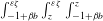$\int _{-1+{\it\beta}b}^{{\it\varepsilon}{\it\zeta}}\int _{z}^{{\it\varepsilon}{\it\zeta}}\int _{-1+{\it\beta}b}^{z}$ to (2.42). The resulting equation is

(4.23) $$\begin{eqnarray}\partial _{t}(h^{3}V^{\sharp })+{\it\varepsilon}\overline{V}\boldsymbol{\cdot }\boldsymbol{{\rm\nabla}}(h^{3}V^{\sharp })+{\it\varepsilon}h^{3}V^{\sharp }\boldsymbol{\cdot }\boldsymbol{{\rm\nabla}}\overline{V}=-3{\it\varepsilon}h^{3}V^{\sharp }\boldsymbol{{\rm\nabla}}\boldsymbol{\cdot }\overline{V}+O({\it\varepsilon}\sqrt{{\it\mu}}).\end{eqnarray}$$

Making use of the identity $\partial _{t}h+{\it\varepsilon}\boldsymbol{{\rm\nabla}}\boldsymbol{\cdot }(h\overline{V})=0$ , this yields

(4.24) $$\begin{eqnarray}\partial _{t}V^{\sharp }+{\it\varepsilon}\overline{V}\boldsymbol{\cdot }\boldsymbol{{\rm\nabla}}V^{\sharp }+{\it\varepsilon}V^{\sharp }\boldsymbol{\cdot }\boldsymbol{{\rm\nabla}}\overline{V}=O({\it\varepsilon}\sqrt{{\it\mu}}),\end{eqnarray}$$

which is the desired closure equation.

4.5. Closure equations for $\boldsymbol{\mathsf{E}}$

Since $\boldsymbol{\mathsf{E}}$ appears in an order $O({\it\mu})$ term in (4.21), we need to derive an equation for $\boldsymbol{\mathsf{E}}$ at precision $O({\it\mu})$ to preserve the overall $O({\it\mu}^{2})$ precision of (4.21). The first step is to derive a more precise equation for the shear velocity $V_{sh}^{\ast }$ that takes into account the $O(\sqrt{{\it\mu}})$ neglected in (2.42). An equation for $\boldsymbol{\mathsf{E}}$ is then deduced from this equation.

4.5.1. An equation for $V_{sh}^{\ast }$ at order $O({\it\mu})$

For later use, we perform directly the computations in the two-dimensional case $d=2$ here, as the adaptations to the case $d=1$ are straightforward.

A more precise version of (2.36) is obtained by making more explicit the $O({\it\varepsilon}\sqrt{{\it\mu}})$ term on the right-hand side; more precisely, we substitute $O({\it\varepsilon}\sqrt{{\it\mu}})$ in (2.36) by

(4.25) $$\begin{eqnarray}\displaystyle & & \displaystyle {\it\varepsilon}\sqrt{{\it\mu}}\Bigg\{-V_{sh}^{\ast }\boldsymbol{\cdot }\boldsymbol{{\rm\nabla}}{\bf\omega}_{{\it\mu},h}+\left(\boldsymbol{{\rm\nabla}}\boldsymbol{\cdot }\int _{-1+{\it\beta}b}^{z}V_{sh}^{\ast }\right)\partial _{z}{\bf\omega}_{{\it\mu},h}+{\bf\omega}_{{\it\mu},h}\boldsymbol{\cdot }\boldsymbol{{\rm\nabla}}V_{sh}^{\ast }\nonumber\\ \displaystyle & & \displaystyle \qquad \quad +\,\boldsymbol{{\rm\nabla}}^{\bot }\boldsymbol{\cdot }\overline{V}\partial _{z}T^{\ast }\overline{V}+\boldsymbol{{\rm\nabla}}^{\bot }\boldsymbol{\cdot }V_{sh}^{\ast }\partial _{z}V_{sh}^{\ast }\Bigg\}+O({\it\varepsilon}{\it\mu}).\end{eqnarray}$$

Consequently, we include the $O(\sqrt{{\it\mu}})$ terms in (2.40) to obtain

(4.26) $$\begin{eqnarray}\partial _{t}V_{sh}+{\it\varepsilon}\overline{V}\boldsymbol{\cdot }\boldsymbol{{\rm\nabla}}V_{sh}+{\it\varepsilon}V_{sh}\boldsymbol{\cdot }\boldsymbol{{\rm\nabla}}\overline{V}-{\it\varepsilon}\boldsymbol{{\rm\nabla}}\boldsymbol{\cdot }[(1+z-{\it\beta}b)\overline{V}]\partial _{z}V_{sh}={\it\varepsilon}\sqrt{{\it\mu}}C+O({\it\varepsilon}{\it\mu}),\end{eqnarray}$$

with

(4.27) $$\begin{eqnarray}\displaystyle C & = & \displaystyle -\int _{z}^{{\it\varepsilon}{\it\zeta}}V_{sh}^{\ast }\boldsymbol{\cdot }\boldsymbol{{\rm\nabla}}{\bf\omega}_{{\it\mu},h}^{\bot }-\int _{z}^{{\it\varepsilon}{\it\zeta}}(\boldsymbol{{\rm\nabla}}\boldsymbol{\cdot }V_{sh}^{\ast }){\bf\omega}_{{\it\mu},h}^{\bot }+\left[\left(\boldsymbol{{\rm\nabla}}\boldsymbol{\cdot }\int _{-1+{\it\beta}b}^{z}V_{sh}^{\ast }\right){\bf\omega}_{{\it\mu},h}^{\bot }\right]_{z}^{{\it\varepsilon}{\it\zeta}}\nonumber\\ \displaystyle & & \displaystyle +\,\int _{z}^{{\it\varepsilon}{\it\zeta}}{\bf\omega}_{{\it\mu},h}\boldsymbol{\cdot }\boldsymbol{{\rm\nabla}}(V_{sh}^{\ast })^{\bot }+\int _{z}^{{\it\varepsilon}{\it\zeta}}\boldsymbol{{\rm\nabla}}^{\bot }\boldsymbol{\cdot }\overline{V}(\partial _{z}T^{\ast }\overline{V})^{\bot }+\int _{z}^{{\it\varepsilon}{\it\zeta}}\boldsymbol{{\rm\nabla}}^{\bot }\boldsymbol{\cdot }V_{sh}^{\ast }\partial _{z}{V_{sh}^{\ast }}^{\bot }.\end{eqnarray}$$

Using (2.39) and since ${\bf\omega}_{{\it\mu},h}^{\bot }=-\partial _{z}V_{sh}^{\ast }$ , this yields

(4.28) $$\begin{eqnarray}\displaystyle C & = & \displaystyle -\int _{z}^{{\it\varepsilon}{\it\zeta}}V_{sh}^{\ast }\boldsymbol{\cdot }\boldsymbol{{\rm\nabla}}{\bf\omega}_{{\it\mu},h}^{\bot }-\int _{z}^{{\it\varepsilon}{\it\zeta}}{\bf\omega}_{{\it\mu},h}^{\bot }\boldsymbol{\cdot }\boldsymbol{{\rm\nabla}}V_{sh}^{\ast }\nonumber\\ \displaystyle & & \displaystyle +\,\left[\left(\boldsymbol{{\rm\nabla}}\boldsymbol{\cdot }\int _{-1+{\it\beta}b}^{z}V_{sh}^{\ast }\right){\bf\omega}_{{\it\mu},h}^{\bot }\right]_{z}^{{\it\varepsilon}{\it\zeta}}+\int _{z}^{{\it\varepsilon}{\it\zeta}}\boldsymbol{{\rm\nabla}}^{\bot }\boldsymbol{\cdot }\overline{V}(\partial _{z}T^{\ast }\overline{V})^{\bot }.\end{eqnarray}$$

Using again that ${\bf\omega}_{{\it\mu},h}^{\bot }=-\partial _{z}V_{sh}^{\ast }$ , we deduce that

(4.29) $$\begin{eqnarray}\displaystyle C & = & \displaystyle \int _{z}^{{\it\varepsilon}{\it\zeta}}\partial _{z}(V_{sh}^{\ast }\boldsymbol{\cdot }\boldsymbol{{\rm\nabla}}V_{sh}^{\ast })+\left[\left(\boldsymbol{{\rm\nabla}}\boldsymbol{\cdot }\int _{-1+{\it\beta}b}^{z}V_{sh}^{\ast }\right){\bf\omega}_{{\it\mu},h}^{\bot }\right]_{z}^{{\it\varepsilon}{\it\zeta}}+\int _{z}^{{\it\varepsilon}{\it\zeta}}\boldsymbol{{\rm\nabla}}^{\bot }\boldsymbol{\cdot }\overline{V}(\partial _{z}T^{\ast }\overline{V})^{\bot }\nonumber\\ \displaystyle & = & \displaystyle -V_{sh}^{\ast }\boldsymbol{\cdot }\boldsymbol{{\rm\nabla}}V_{sh}^{\ast }+\overline{V}_{sh}\boldsymbol{\cdot }\boldsymbol{{\rm\nabla}}\overline{V}_{sh}+\left(\boldsymbol{{\rm\nabla}}\boldsymbol{\cdot }\int _{-1+{\it\beta}b}^{z}V_{sh}^{\ast }\right)\partial _{z}V_{sh}^{\ast }-\boldsymbol{{\rm\nabla}}^{\bot }\boldsymbol{\cdot }\overline{V}(T\overline{V})^{\bot }.\end{eqnarray}$$

Finally, we have, therefore, the following higher-order version of (2.40):

(4.30) $$\begin{eqnarray}\displaystyle & & \displaystyle \partial _{t}V_{sh}+{\it\varepsilon}\overline{V}\boldsymbol{\cdot }\boldsymbol{{\rm\nabla}}V_{sh}+{\it\varepsilon}V_{sh}\boldsymbol{\cdot }\boldsymbol{{\rm\nabla}}\overline{V}+{\it\varepsilon}\sqrt{{\it\mu}}(V_{sh}^{\ast }\boldsymbol{\cdot }\boldsymbol{{\rm\nabla}}V_{sh}-V_{sh}\boldsymbol{\cdot }\boldsymbol{{\rm\nabla}}\overline{V}_{sh})\nonumber\\ \displaystyle & & \displaystyle \quad ={\it\varepsilon}\boldsymbol{{\rm\nabla}}\boldsymbol{\cdot }\left[\int _{-1+{\it\beta}b}^{z}(\overline{V}+\sqrt{{\it\mu}}V_{sh}^{\ast })\right]\partial _{z}V_{sh}^{\ast }-{\it\varepsilon}\sqrt{{\it\mu}}\boldsymbol{{\rm\nabla}}^{\bot }\boldsymbol{\cdot }\overline{V}(T\overline{V})^{\bot }+O({\it\varepsilon}{\it\mu}).\end{eqnarray}$$

Integrating this yields the following equation for the shear velocity $\overline{V}_{sh}$ :

(4.31) $$\begin{eqnarray}\displaystyle & & \displaystyle \partial _{t}\overline{V}_{sh}+{\it\varepsilon}\overline{V}\boldsymbol{\cdot }\boldsymbol{{\rm\nabla}}\overline{V}_{sh}+{\it\varepsilon}\overline{V}_{sh}\boldsymbol{\cdot }\boldsymbol{{\rm\nabla}}\overline{V}+{\it\varepsilon}\sqrt{{\it\mu}}\frac{1}{h}\boldsymbol{{\rm\nabla}}\boldsymbol{\cdot }\int _{-1+{\it\beta}b}^{{\it\varepsilon}{\it\zeta}}V_{sh}^{\ast }\otimes V_{sh}^{\ast }-{\it\varepsilon}\sqrt{{\it\mu}}\overline{V}_{sh}\boldsymbol{\cdot }\boldsymbol{{\rm\nabla}}\overline{V}_{sh}\nonumber\\ \displaystyle & & \displaystyle \quad =-{\it\varepsilon}\sqrt{{\it\mu}}\boldsymbol{{\rm\nabla}}^{\bot }\boldsymbol{\cdot }\overline{V}(\overline{T}\overline{V})^{\bot }+O({\it\varepsilon}{\it\mu}).\end{eqnarray}$$

Taking the difference of these two equations, and dropping the $O({\it\mu})$ terms, we obtain the following higher-order generalization of (2.42):

(4.32) $$\begin{eqnarray}\displaystyle & & \displaystyle \partial _{t}V_{sh}^{\ast }+{\it\varepsilon}\overline{V}\boldsymbol{\cdot }\boldsymbol{{\rm\nabla}}V_{sh}^{\ast }+{\it\varepsilon}V_{sh}^{\ast }\boldsymbol{\cdot }\boldsymbol{{\rm\nabla}}\overline{V}+{\it\varepsilon}\sqrt{{\it\mu}}\left(V_{sh}^{\ast }\boldsymbol{\cdot }\boldsymbol{{\rm\nabla}}V_{sh}^{\ast }-\frac{1}{h}\boldsymbol{{\rm\nabla}}\boldsymbol{\cdot }\int _{-1+{\it\beta}b}^{{\it\varepsilon}{\it\zeta}}V_{sh}^{\ast }\otimes V_{sh}^{\ast }\right)\nonumber\\ \displaystyle & & \displaystyle \quad ={\it\varepsilon}\boldsymbol{{\rm\nabla}}\boldsymbol{\cdot }\left[\int _{-1+{\it\beta}b}^{z}(\overline{V}+\sqrt{{\it\mu}}V_{sh}^{\ast })\right]\partial _{z}V_{sh}^{\ast }-{\it\varepsilon}\sqrt{{\it\mu}}\boldsymbol{{\rm\nabla}}^{\bot }\boldsymbol{\cdot }\overline{V}(T^{\ast }\overline{V})^{\bot }.\end{eqnarray}$$

4.5.2. An equation for $\boldsymbol{\mathsf{E}}$

In dimension $d=1$ , (4.32) takes the form

(4.33) $$\begin{eqnarray}\displaystyle & & \displaystyle \partial _{t}v_{sh}^{\ast }+{\it\varepsilon}\overline{v}\partial _{x}v_{sh}^{\ast }+{\it\varepsilon}v_{sh}^{\ast }\partial _{x}\overline{v}+{\it\varepsilon}\sqrt{{\it\mu}}\left(v_{sh}^{\ast }\partial _{x}v_{sh}^{\ast }-\frac{1}{h}\partial _{x}\int _{-1+{\it\beta}b}^{{\it\varepsilon}{\it\zeta}}|v_{sh}^{\ast }|^{2}\right)\nonumber\\ \displaystyle & & \displaystyle \quad ={\it\varepsilon}\partial _{x}\left[\int _{-1+{\it\beta}b}^{z}(\overline{v}+\sqrt{{\it\mu}}v_{sh}^{\ast })\right]\partial _{z}v_{sh}^{\ast }.\end{eqnarray}$$

An equation for $\boldsymbol{\mathsf{E}}$ is simply obtained by multiplying this equation by $v_{sh}^{\ast }$ and integrating in $z$ ,

(4.34) $$\begin{eqnarray}\partial _{t}\boldsymbol{\mathsf{E}}+{\it\varepsilon}\overline{v}\partial _{x}\boldsymbol{\mathsf{E}}+3{\it\varepsilon}\boldsymbol{\mathsf{E}}\partial _{x}\overline{v}+{\it\varepsilon}\sqrt{{\it\mu}}\partial _{x}\boldsymbol{\mathsf{F}}=0\end{eqnarray}$$

(up to $O({\it\varepsilon}{\it\mu})$ terms), with

(4.35) $$\begin{eqnarray}\boldsymbol{\mathsf{F}}=\int _{-1+{\it\beta}b}^{{\it\varepsilon}{\it\zeta}}(v_{sh}^{\ast })^{3}.\end{eqnarray}$$

Clearly, $\boldsymbol{\mathsf{F}}$ cannot be determined in terms of ${\it\zeta}$ , $\overline{v}$ , $v^{\sharp }$ and $\boldsymbol{\mathsf{E}}$ , and a last equation is therefore needed.

4.5.3. An equation for $\boldsymbol{\mathsf{F}}$

Since $\boldsymbol{\mathsf{F}}$ appears only in the $O(\sqrt{{\it\mu}})$ term in (4.34), we just need to determine an evolution equation for $\boldsymbol{\mathsf{F}}$ up to $O(\sqrt{{\it\mu}})$ terms. This equation is easily obtained by multiplying (2.42) by $|v_{sh}^{\ast }|^{2}$ and integrating vertically,

(4.36) $$\begin{eqnarray}\partial _{t}\boldsymbol{\mathsf{F}}+{\it\varepsilon}\overline{v}\partial _{x}\boldsymbol{\mathsf{F}}+4{\it\varepsilon}\boldsymbol{\mathsf{F}}\partial _{x}\overline{v}=0\end{eqnarray}$$

(up to $O({\it\varepsilon}\sqrt{{\it\mu}})$ terms).

4.6. The Green–Naghdi model

We are now able to give the Green–Naghdi equations in dimension $d=1$ , with general vorticity, and for non-flat bottoms of medium amplitude (i.e.  ${\it\beta}=O(\sqrt{{\it\mu}})$ ). These equations are an order $O({\it\mu}^{2})$ approximation of (2.15), where the momentum equation is approximated by (4.21) which involves a rotational energy $\boldsymbol{\mathsf{E}}$ determined through the finite cascade (4.34), (4.36). More precisely, we have, dropping $O({\it\mu}^{2})$ terms,

(4.37) $$\begin{eqnarray}\left.\begin{array}{@{}c@{}}\partial _{t}{\it\zeta}+\partial _{x}(h\overline{v})=0,\\ \displaystyle (1+{\it\mu}\mathscr{T})(\partial _{t}\overline{v}+{\it\varepsilon}\overline{v}\partial _{x}\overline{v})+\partial _{x}{\it\zeta}+{\it\varepsilon}{\it\mu}\mathscr{Q}_{1}(\overline{v})+{\it\varepsilon}{\it\mu}\frac{1}{h}\partial _{x}\boldsymbol{\mathsf{E}}+{\it\varepsilon}{\it\mu}^{3/2}\mathscr{C}(v^{\sharp },\overline{v})=0,\\ \partial _{t}v^{\sharp }+{\it\varepsilon}\overline{v}\partial _{x}v^{\sharp }+{\it\varepsilon}v^{\sharp }\partial _{x}\overline{v}=0,\\ \partial _{t}\boldsymbol{\mathsf{E}}+{\it\varepsilon}\overline{v}\partial _{x}\boldsymbol{\mathsf{E}}+3{\it\varepsilon}\boldsymbol{\mathsf{E}}\partial _{x}\overline{v}+{\it\varepsilon}\sqrt{{\it\mu}}\partial _{x}\boldsymbol{\mathsf{F}}=0,\\ \partial _{t}\boldsymbol{\mathsf{F}}+{\it\varepsilon}\overline{v}\partial _{x}\boldsymbol{\mathsf{F}}+4{\it\varepsilon}\boldsymbol{\mathsf{F}}\partial _{x}\overline{v}=0,\end{array}\right\}\end{eqnarray}$$

where $\mathscr{T}$ , $\mathscr{Q}_{1}$ and $\mathscr{C}$ are defined in (1.16), (1.17) and (3.10) respectively, while we recall that $\boldsymbol{\mathsf{E}}$ , $\boldsymbol{\mathsf{F}}$ and $v^{\sharp }$ stand for

(4.38a−c ) $$\begin{eqnarray}\boldsymbol{\mathsf{E}}=\int _{-1+{\it\beta}b}^{{\it\varepsilon}{\it\zeta}}(v_{sh}^{\ast })^{2},\quad \boldsymbol{\mathsf{F}}=\int _{-1+{\it\beta}b}^{{\it\varepsilon}{\it\zeta}}(v_{sh}^{\ast })^{3}\quad \text{and}\quad v^{\sharp }=-\frac{24}{h^{3}}\int _{-1+{\it\beta}b}^{{\it\varepsilon}{\it\zeta}}\int _{z}^{{\it\varepsilon}{\it\zeta}}\int _{-1+{\it\beta}b}^{z}v_{sh}^{\ast }.\end{eqnarray}$$

Remark 10. By simple integrations by parts, it is possible to rewrite $v^{\sharp }$ as a second-order momentum,

(4.39) $$\begin{eqnarray}v^{\sharp }=\frac{12}{h^{3}}\int _{-1+{\it\beta}b}^{{\it\varepsilon}{\it\zeta}}(z+1-{\it\beta}b)^{2}v_{sh}^{\ast }.\end{eqnarray}$$

Remark 11. As in Remark 9 for the case of constant vorticity, a local equation for the conservation of energy can be derived, which generalizes (1.19) and (3.13), namely,

(4.40) $$\begin{eqnarray}\partial _{t}(\mathfrak{e}+\mathfrak{e}_{rot})+\partial _{x}(\mathfrak{F}+\mathfrak{F}_{rot})=0,\end{eqnarray}$$

with (in dimensional form)

(4.41a,b ) $$\begin{eqnarray}\mathfrak{e}_{rot}={\textstyle \frac{1}{2}}\boldsymbol{\mathsf{E}}\quad \text{and}\quad \mathfrak{F}_{rot}={\textstyle \frac{3}{2}}\boldsymbol{\mathsf{E}}\,\overline{v}+{\textstyle \frac{1}{2}}\boldsymbol{\mathsf{F}}+\mathfrak{F}_{\mathscr{C}},\end{eqnarray}$$

the flux $\mathfrak{F}_{\mathscr{C}}$ being as in Remark 8.

Remark 12. No smallness assumption on ${\it\varepsilon}$ has been made to derive (4.37). Assuming that ${\it\varepsilon}=\sqrt{{\it\mu}}$ (medium-amplitude waves with the terminology of Lannes (Reference Lannes2013)), one can simplify (4.37) by dropping $O({\it\mu}^{2})$ terms. This yields

(4.42) $$\begin{eqnarray}\left.\begin{array}{@{}l@{}}\partial _{t}{\it\zeta}+\partial _{x}(h\overline{v})=0,\\ (1+{\it\mu}\mathscr{T})(\partial _{t}\overline{v}+{\it\varepsilon}\overline{v}\partial _{x}\overline{v})+\partial _{x}{\it\zeta}+{\it\varepsilon}{\it\mu}\mathscr{Q}_{1}(\overline{v})+{\it\varepsilon}{\it\mu}\partial _{x}\boldsymbol{\mathsf{E}}=0,\\ \partial _{t}\boldsymbol{\mathsf{E}}+{\it\varepsilon}\overline{v}\partial _{x}\boldsymbol{\mathsf{E}}+3{\it\varepsilon}\boldsymbol{\mathsf{E}}\partial _{x}\overline{v}=0.\end{array}\right\}\end{eqnarray}$$

5.1. Computation of the ‘rotational Reynolds tensor’ contribution

Proceeding as for (3.4) and (4.7), we write, up to $O({\it\mu}^{2})$ terms,

(5.4) $$\begin{eqnarray}\displaystyle {\it\varepsilon}{\it\mu}\boldsymbol{{\rm\nabla}}\boldsymbol{\cdot }\int _{-1+{\it\beta}b}^{{\it\varepsilon}{\it\zeta}}V^{\ast }\otimes V^{\ast } & = & \displaystyle {\it\varepsilon}{\it\mu}\boldsymbol{{\rm\nabla}}\boldsymbol{\cdot }\int _{-1+{\it\beta}b}^{{\it\varepsilon}{\it\zeta}}V_{sh}^{\ast }\otimes V_{sh}^{\ast }\nonumber\\ \displaystyle & & \displaystyle -\,{\it\varepsilon}{\it\mu}^{3/2}\frac{1}{2}\boldsymbol{{\rm\nabla}}\boldsymbol{\cdot }\int _{-1+{\it\beta}b}^{{\it\varepsilon}{\it\zeta}}\int _{z}^{{\it\varepsilon}{\it\zeta}}\boldsymbol{{\rm\nabla}}\boldsymbol{{\rm\nabla}}\boldsymbol{\cdot }((1+z-{\it\beta}b)\overline{V})\otimes V_{sh}^{\ast }\nonumber\\ \displaystyle & & \displaystyle -\,{\it\varepsilon}{\it\mu}^{3/2}\frac{1}{2}\boldsymbol{{\rm\nabla}}\boldsymbol{\cdot }\int _{-1+{\it\beta}b}^{{\it\varepsilon}{\it\zeta}}\int _{z}^{{\it\varepsilon}{\it\zeta}}V_{sh}^{\ast }\otimes \boldsymbol{{\rm\nabla}}\boldsymbol{{\rm\nabla}}\boldsymbol{\cdot }((1+z-{\it\beta}b)\overline{V}).\nonumber\\ \displaystyle & & \displaystyle\end{eqnarray}$$

Introducing

(5.5) $$\begin{eqnarray}V^{\sharp }=\frac{24}{h^{3}}\int _{-1+{\it\beta}b}^{{\it\varepsilon}{\it\zeta}}\int _{z}^{{\it\varepsilon}{\it\zeta}}\int _{-1+{\it\beta}b}^{z}V_{sh}^{\ast }\end{eqnarray}$$

and proceeding as in § 4.1, we obtain

(5.6) $$\begin{eqnarray}\displaystyle & \displaystyle {\it\varepsilon}{\it\mu}\boldsymbol{{\rm\nabla}}\boldsymbol{\cdot }\int _{-1+{\it\beta}b}^{{\it\varepsilon}{\it\zeta}}V^{\ast }\otimes V^{\ast }={\it\varepsilon}{\it\mu}\boldsymbol{{\rm\nabla}}\boldsymbol{\cdot }\int _{-1+{\it\beta}b}^{{\it\varepsilon}{\it\zeta}}V_{sh}^{\ast }\otimes V_{sh}^{\ast } & \displaystyle \nonumber\\ \displaystyle & \displaystyle \quad -\,{\it\varepsilon}{\it\mu}^{3/2}\frac{1}{24}\boldsymbol{{\rm\nabla}}\boldsymbol{\cdot }h^{3}V^{\sharp }\otimes \boldsymbol{{\rm\nabla}}\boldsymbol{{\rm\nabla}}\boldsymbol{\cdot }\overline{V}+\boldsymbol{{\rm\nabla}}\boldsymbol{{\rm\nabla}}\boldsymbol{\cdot }\overline{V}\otimes V^{\sharp }+O({\it\mu}^{2}). & \displaystyle\end{eqnarray}$$

5.2. Computation of the pressure contribution

As for (3.5) and (4.8), we have

(5.7) $$\begin{eqnarray}\displaystyle \frac{1}{{\it\varepsilon}}\int _{-1+{\it\beta}b}^{{\it\varepsilon}{\it\zeta}}\boldsymbol{{\rm\nabla}}p & = & \displaystyle h\boldsymbol{{\rm\nabla}}{\it\zeta}+\int _{-1+{\it\beta}b}^{{\it\varepsilon}{\it\zeta}}\boldsymbol{{\rm\nabla}}\int _{z}^{{\it\varepsilon}{\it\zeta}}\left(\partial _{t}w+{\it\varepsilon}V\boldsymbol{\cdot }\boldsymbol{{\rm\nabla}}w+\frac{{\it\varepsilon}}{{\it\mu}}w\partial _{z}w\right)\nonumber\\ \displaystyle & = & \displaystyle h\boldsymbol{{\rm\nabla}}{\it\zeta}+{\it\mu}A_{(1)}+{\it\mu}^{3/2}A_{(3/2)}+O({\it\mu}^{2}),\end{eqnarray}$$

where, as in the irrotational case,

(5.8) $$\begin{eqnarray}A_{(1)}=h\mathscr{T}(\partial _{t}\overline{V}+{\it\varepsilon}\overline{V}\boldsymbol{\cdot }\boldsymbol{{\rm\nabla}}\overline{V})+{\it\varepsilon}h\mathscr{Q}_{1}(\overline{V}),\end{eqnarray}$$

and $\mathscr{Q}_{1}(\overline{V})$ as in (1.17). For the $O({\it\mu}^{3/2})$ component, we have

(5.9) $$\begin{eqnarray}\displaystyle A_{(3/2)} & = & \displaystyle h\widetilde{\mathscr{T}}(\partial _{t}V_{sh}^{\ast }+{\it\varepsilon}\overline{V}\boldsymbol{\cdot }\boldsymbol{{\rm\nabla}}V_{sh}^{\ast })+2{\it\varepsilon}\int _{-1}^{{\it\varepsilon}{\it\zeta}}\boldsymbol{{\rm\nabla}}\int _{z}^{{\it\varepsilon}{\it\zeta}}\left(\int _{-1}^{z}\boldsymbol{{\rm\nabla}}\boldsymbol{\cdot }V_{sh}^{\ast }\right)\boldsymbol{{\rm\nabla}}\boldsymbol{\cdot }\overline{V}\nonumber\\ \displaystyle & & \displaystyle -\,{\it\varepsilon}\int _{-1}^{{\it\varepsilon}{\it\zeta}}\boldsymbol{{\rm\nabla}}\int _{z}^{{\it\varepsilon}{\it\zeta}}V_{sh}^{\ast }\boldsymbol{\cdot }\boldsymbol{{\rm\nabla}}(\boldsymbol{{\rm\nabla}}\boldsymbol{\cdot }((1+z^{\prime })\overline{V}))+{\it\varepsilon}\int _{-1}^{{\it\varepsilon}{\it\zeta}}\boldsymbol{{\rm\nabla}}\int _{z}^{{\it\varepsilon}{\it\zeta}}\boldsymbol{{\rm\nabla}}\boldsymbol{\cdot }((1+z)\overline{V})\boldsymbol{{\rm\nabla}}\boldsymbol{\cdot }V_{sh}^{\ast }\nonumber\\ \displaystyle & & \displaystyle +\,{\it\varepsilon}\int _{-1}^{{\it\varepsilon}{\it\zeta}}\boldsymbol{{\rm\nabla}}\int _{z}^{{\it\varepsilon}{\it\zeta}}([\text{div},\overline{V}\boldsymbol{\cdot }\boldsymbol{{\rm\nabla}}]-(\boldsymbol{{\rm\nabla}}\boldsymbol{\cdot }\overline{V})\boldsymbol{{\rm\nabla}}^{\text{T}})\int _{-1}^{z}V_{sh}^{\ast }.\end{eqnarray}$$

Applying $\widetilde{\mathscr{T}}$ to (2.42) to handle the first term on the right-hand side, we obtain, proceeding as in § 4.2, that

(5.10) $$\begin{eqnarray}\displaystyle A_{(3/2)} & = & \displaystyle -{\it\varepsilon}h\widetilde{\mathscr{T}}(V_{sh}^{\ast }\boldsymbol{\cdot }\boldsymbol{{\rm\nabla}}\overline{V}+V_{sh}^{\ast }\boldsymbol{{\rm\nabla}}\boldsymbol{\cdot }\overline{V})+2{\it\varepsilon}\int _{-1}^{{\it\varepsilon}{\it\zeta}}\boldsymbol{{\rm\nabla}}\int _{z}^{{\it\varepsilon}{\it\zeta}}\left(\int _{-1}^{z}\boldsymbol{{\rm\nabla}}\boldsymbol{\cdot }V_{sh}^{\ast }\right)\boldsymbol{{\rm\nabla}}\boldsymbol{\cdot }\overline{V}\nonumber\\ \displaystyle & & \displaystyle -\,2{\it\varepsilon}\int _{-1}^{{\it\varepsilon}{\it\zeta}}\boldsymbol{{\rm\nabla}}\int _{z}^{{\it\varepsilon}{\it\zeta}}V_{sh}^{\ast }\boldsymbol{\cdot }\boldsymbol{{\rm\nabla}}(\boldsymbol{{\rm\nabla}}\boldsymbol{\cdot }((1+z^{\prime })\overline{V}))\nonumber\\ \displaystyle & & \displaystyle +\,{\it\varepsilon}\int _{-1}^{{\it\varepsilon}{\it\zeta}}\boldsymbol{{\rm\nabla}}\int _{z}^{{\it\varepsilon}{\it\zeta}}([\text{div},\overline{V}\boldsymbol{\cdot }\boldsymbol{{\rm\nabla}}]-(\boldsymbol{{\rm\nabla}}\boldsymbol{\cdot }\overline{V})\boldsymbol{{\rm\nabla}}^{\text{T}})\int _{-1}^{z}V_{sh}^{\ast }\nonumber\\ \displaystyle & = & \displaystyle -{\it\varepsilon}\boldsymbol{{\rm\nabla}}\left[\frac{h^{3}}{4}V_{sh}^{\ast }\boldsymbol{\cdot }\boldsymbol{{\rm\nabla}}\boldsymbol{{\rm\nabla}}\boldsymbol{\cdot }\overline{V}+\frac{1}{12}\boldsymbol{{\rm\nabla}}\boldsymbol{\cdot }\overline{V}\boldsymbol{{\rm\nabla}}\boldsymbol{\cdot }(h^{3}V_{sh}^{\ast })+\frac{1}{12}\text{Tr}(\boldsymbol{{\rm\nabla}}\overline{V}\boldsymbol{{\rm\nabla}}(h^{3}V^{\sharp }))\right].\qquad \nonumber\\ \displaystyle & & \displaystyle\end{eqnarray}$$

5.3. Wave–current interaction in the velocity equation

From the momentum equation in (2.15) and (5.6)–(5.8) and (5.10), we obtain

(5.11) $$\begin{eqnarray}\left(1+{\it\mu}\mathscr{T}\right)(\partial _{t}\overline{V}+{\it\varepsilon}\overline{V}\boldsymbol{\cdot }\boldsymbol{{\rm\nabla}}\overline{V})+{\it\mu}{\it\varepsilon}\mathscr{Q}_{1}(\overline{V})+{\it\varepsilon}{\it\mu}\frac{1}{h}\boldsymbol{{\rm\nabla}}\boldsymbol{\cdot }\boldsymbol{\mathsf{E}}+{\it\varepsilon}{\it\mu}^{3/2}\mathscr{C}(V^{\sharp },\overline{V})=0,\end{eqnarray}$$

where

(5.12a,b ) $$\begin{eqnarray}\boldsymbol{\mathsf{E}}=\int _{-1+{\it\beta}b}^{{\it\varepsilon}{\it\zeta}}V_{sh}^{\ast }\otimes V_{sh}^{\ast }\quad \text{and}\quad V^{\sharp }=-\frac{24}{h^{3}}\int _{-1+{\it\beta}b}^{{\it\varepsilon}{\it\zeta}}\int _{z}^{{\it\varepsilon}{\it\zeta}}\int _{-1+{\it\beta}b}^{z}V_{sh}^{\ast },\end{eqnarray}$$

and where $\mathscr{C}(V^{\sharp },\overline{V})$ is the two-dimensional generalization of (3.10),

(5.13) $$\begin{eqnarray}\displaystyle & \displaystyle \mathscr{C}(V^{\sharp },\overline{V})=-\frac{1}{24h}\boldsymbol{{\rm\nabla}}\boldsymbol{\cdot }(h^{3}(V^{\sharp }\otimes \boldsymbol{{\rm\nabla}}\boldsymbol{{\rm\nabla}}\boldsymbol{\cdot }\overline{V}+\boldsymbol{{\rm\nabla}}\boldsymbol{{\rm\nabla}}\boldsymbol{\cdot }\overline{V}\otimes V^{\sharp })) & \displaystyle \nonumber\\ \displaystyle & \displaystyle \quad -\frac{1}{4h}\boldsymbol{{\rm\nabla}}\left[h^{3}V^{\sharp }\boldsymbol{\cdot }\boldsymbol{{\rm\nabla}}\boldsymbol{{\rm\nabla}}\boldsymbol{\cdot }\overline{V}+\frac{1}{3}\boldsymbol{{\rm\nabla}}\boldsymbol{\cdot }\overline{V}\boldsymbol{{\rm\nabla}}\boldsymbol{\cdot }(h^{3}V^{\sharp })+\frac{1}{3}\text{Tr}(\boldsymbol{{\rm\nabla}}\overline{V}\boldsymbol{{\rm\nabla}}(h^{3}V^{\sharp }))\right]. & \displaystyle\end{eqnarray}$$

As in the one-dimensional case (see § 4.3), closure equations are needed for $V^{\sharp }$ and $\boldsymbol{\mathsf{E}}$ . The closure equation has already been derived in the two-dimensional case in § 4.4; it is given by

(5.14) $$\begin{eqnarray}\partial _{t}V^{\sharp }+{\it\varepsilon}(\overline{V}\boldsymbol{\cdot }\boldsymbol{{\rm\nabla}})V^{\sharp }+{\it\varepsilon}(V^{\sharp }\boldsymbol{\cdot }\boldsymbol{{\rm\nabla}})\overline{V}=0.\end{eqnarray}$$

The derivation of the closure equation for $\boldsymbol{\mathsf{E}}$ is addressed in the following section.

5.4. Closure equation for $\boldsymbol{\mathsf{E}}$

We first derive an equation for $\boldsymbol{\mathsf{E}}$ , which involves a third-order tensor $\boldsymbol{\mathsf{F}}$ , for which we also derive an equation that closes the system.

5.4.1. An equation for $\boldsymbol{\mathsf{E}}$

Recall first that we obtained in (4.32) an evolution equation for $V_{sh}^{\ast }$ , namely

(5.15) $$\begin{eqnarray}\partial _{t}V_{sh}^{\ast }+{\it\varepsilon}\overline{V}\boldsymbol{\cdot }\boldsymbol{{\rm\nabla}}V_{sh}^{\ast }+{\it\varepsilon}V_{sh}^{\ast }\boldsymbol{\cdot }\boldsymbol{{\rm\nabla}}\overline{V}={\it\varepsilon}\boldsymbol{{\rm\nabla}}\boldsymbol{\cdot }((1+z-{\it\beta}b)\overline{V})\partial _{z}V_{sh}^{\ast }+{\it\varepsilon}\sqrt{{\it\mu}}C^{\ast },\end{eqnarray}$$

with

(5.16) $$\begin{eqnarray}C^{\ast }=-V_{sh}^{\ast }\boldsymbol{\cdot }\boldsymbol{{\rm\nabla}}V_{sh}^{\ast }+\frac{1}{h}\boldsymbol{{\rm\nabla}}\boldsymbol{\cdot }\int _{-1+{\it\beta}b}^{{\it\varepsilon}{\it\zeta}}V_{sh}^{\ast }\otimes V_{sh}^{\ast }+\boldsymbol{{\rm\nabla}}\boldsymbol{\cdot }\left(\int _{-1+{\it\beta}b}^{z}V_{sh}^{\ast }\right)\partial _{z}V_{sh}^{\ast }-\boldsymbol{{\rm\nabla}}^{\bot }\boldsymbol{\cdot }\overline{V}(T^{\ast }\overline{V})^{\bot }.\end{eqnarray}$$

Time differentiating the tensor $\boldsymbol{\mathsf{E}}$ , we obtain therefore

(5.17) $$\begin{eqnarray}\displaystyle \partial _{t}\boldsymbol{\mathsf{E}} & = & \displaystyle \partial _{t}({\it\varepsilon}{\it\zeta})(V_{sh}^{\ast }\otimes V_{sh}^{\ast })_{|_{surf}}+\int _{-1+{\it\beta}b}^{{\it\varepsilon}{\it\zeta}}\left(\partial _{t}V_{sh}^{\ast }\otimes V_{sh}^{\ast }+V_{sh}^{\ast }\otimes \partial _{t}V_{sh}^{\ast }\right)\nonumber\\ \displaystyle & = & \displaystyle \partial _{t}({\it\varepsilon}{\it\zeta})(V_{sh}^{\ast }\otimes V_{sh}^{\ast })_{|_{surf}}+I_{1}+I_{2}+I_{3}+{\it\varepsilon}\sqrt{{\it\mu}}\boldsymbol{\mathsf{G}},\end{eqnarray}$$

with

(5.18) $$\begin{eqnarray}\displaystyle I_{1} & = & \displaystyle -{\it\varepsilon}\int _{-1+{\it\beta}b}^{{\it\varepsilon}{\it\zeta}}\left((\overline{V}\boldsymbol{\cdot }\boldsymbol{{\rm\nabla}})V_{sh}^{\ast }\otimes V_{sh}^{\ast }+V_{sh}^{\ast }\otimes (\overline{V}\boldsymbol{\cdot }\boldsymbol{{\rm\nabla}})V_{sh}^{\ast }\right)\nonumber\\ \displaystyle & = & \displaystyle -{\it\varepsilon}\overline{V}\boldsymbol{\cdot }\boldsymbol{{\rm\nabla}}\boldsymbol{\mathsf{E}}+{\it\varepsilon}(\overline{V}\boldsymbol{\cdot }\boldsymbol{{\rm\nabla}}({\it\varepsilon}{\it\zeta})(V_{sh}^{\ast }\otimes V_{sh}^{\ast })_{|_{surf}}-\overline{V}\boldsymbol{\cdot }\boldsymbol{{\rm\nabla}}({\it\beta}b)(V_{sh}^{\ast }\otimes V_{sh}^{\ast })_{|_{bott}}),\end{eqnarray}$$

while

(5.19) $$\begin{eqnarray}\displaystyle I_{2} & = & \displaystyle \int _{-1+{\it\beta}b}^{{\it\varepsilon}{\it\zeta}}\boldsymbol{{\rm\nabla}}\boldsymbol{\cdot }((1+z-{\it\beta}b)\overline{V})\left(\partial _{z}V_{sh}^{\ast }\otimes V_{sh}^{\ast }+V_{sh}^{\ast }\otimes \partial _{z}V_{sh}^{\ast }\right)\nonumber\\ \displaystyle & = & \displaystyle -\boldsymbol{\mathsf{E}}+h(V_{sh}^{\ast }\otimes V_{sh}^{\ast })_{|_{surf}}-\boldsymbol{{\rm\nabla}}({\it\beta}b)\boldsymbol{\cdot }\overline{V}((V_{sh}^{\ast }\otimes V_{sh}^{\ast })_{|_{surf}}-(V_{sh}^{\ast }\otimes V_{sh}^{\ast })_{|_{bott}})\end{eqnarray}$$

and

(5.20) $$\begin{eqnarray}\displaystyle I_{3} & = & \displaystyle -{\it\varepsilon}\int _{-1+{\it\beta}b}^{{\it\varepsilon}{\it\zeta}}\left((V_{sh}^{\ast }\boldsymbol{\cdot }\boldsymbol{{\rm\nabla}}\overline{V})\otimes V_{sh}^{\ast }+V_{sh}^{\ast }\otimes (V_{sh}^{\ast }\boldsymbol{\cdot }\boldsymbol{{\rm\nabla}})\overline{V}\right)\nonumber\\ \displaystyle & = & \displaystyle -(\boldsymbol{{\rm\nabla}}\overline{V})^{\bot }\boldsymbol{\mathsf{E}}-\boldsymbol{\mathsf{E}}\boldsymbol{{\rm\nabla}}\overline{V}.\end{eqnarray}$$

Finally, the matrix $\boldsymbol{\mathsf{G}}$ is given by

(5.21) $$\begin{eqnarray}\displaystyle \boldsymbol{\mathsf{G}} & = & \displaystyle \int _{-1+{\it\beta}b}^{{\it\varepsilon}{\it\zeta}}C^{\ast }\otimes V_{sh}^{\ast }+V_{sh}^{\ast }\otimes C^{\ast }\nonumber\\ \displaystyle & = & \displaystyle -\int _{-1+{\it\beta}b}^{{\it\varepsilon}{\it\zeta}}(V_{sh}^{\ast }\boldsymbol{\cdot }\boldsymbol{{\rm\nabla}}V_{sh}^{\ast })\otimes V_{sh}^{\ast }+V_{sh}^{\ast }\otimes (V_{sh}^{\ast }\boldsymbol{\cdot }\boldsymbol{{\rm\nabla}}V_{sh}^{\ast })\nonumber\\ \displaystyle & & \displaystyle -\,\int _{-1+{\it\beta}b}^{{\it\varepsilon}{\it\zeta}}(\boldsymbol{{\rm\nabla}}\boldsymbol{\cdot }V_{sh}^{\ast })V_{sh}^{\ast }\otimes V_{sh}^{\ast }-{\it\varepsilon}\boldsymbol{{\rm\nabla}}{\it\zeta}\boldsymbol{\cdot }V_{sh}^{\ast }(V_{sh}^{\ast }\otimes V_{sh}^{\ast })_{|_{surf}}+{\it\beta}\boldsymbol{{\rm\nabla}}b\boldsymbol{\cdot }V_{sh}^{\ast }(V_{sh}^{\ast }\otimes V_{sh}^{\ast })_{|_{bott}}\nonumber\\ \displaystyle & & \displaystyle +\,\frac{h^{4}}{24}(\boldsymbol{{\rm\nabla}}^{\bot }\boldsymbol{\cdot }\overline{V}\boldsymbol{{\rm\nabla}}^{\bot }\boldsymbol{{\rm\nabla}}\boldsymbol{\cdot }\overline{V}\otimes V^{\sharp }+V^{\sharp }\otimes \boldsymbol{{\rm\nabla}}^{\bot }\boldsymbol{\cdot }\overline{V}\boldsymbol{{\rm\nabla}}^{\bot }\boldsymbol{{\rm\nabla}}\boldsymbol{\cdot }\overline{V}).\end{eqnarray}$$

Gathering all these computations, we finally obtain that

(5.22) $$\begin{eqnarray}\partial _{t}\boldsymbol{\mathsf{E}}+{\it\varepsilon}\overline{V}\boldsymbol{\cdot }\boldsymbol{{\rm\nabla}}\boldsymbol{\mathsf{E}}+{\it\varepsilon}\boldsymbol{{\rm\nabla}}\boldsymbol{\cdot }\overline{V}\boldsymbol{\mathsf{E}}+{\it\varepsilon}\boldsymbol{{\rm\nabla}}\overline{V}^{\text{T}}\boldsymbol{\mathsf{E}}+{\it\varepsilon}\boldsymbol{\mathsf{E}}\boldsymbol{{\rm\nabla}}\overline{V}+{\it\varepsilon}\sqrt{{\it\mu}}\boldsymbol{{\rm\nabla}}\boldsymbol{\cdot }\boldsymbol{\mathsf{F}}={\it\varepsilon}\sqrt{{\it\mu}}\mathscr{D}(V^{\sharp },\overline{V}),\end{eqnarray}$$

where

(5.23) $$\begin{eqnarray}\boldsymbol{\mathsf{F}}=\int _{-1+{\it\beta}b}^{{\it\varepsilon}{\it\zeta}}V_{sh}^{\ast }\otimes V_{sh}^{\ast }\otimes V_{sh}^{\ast }\end{eqnarray}$$

and

(5.24) $$\begin{eqnarray}\mathscr{D}(V^{\sharp },\overline{V})=\frac{h^{3}}{24}\boldsymbol{{\rm\nabla}}^{\bot }\boldsymbol{\cdot }\overline{V}(\boldsymbol{{\rm\nabla}}^{\bot }\boldsymbol{{\rm\nabla}}\boldsymbol{\cdot }\overline{V}\otimes V^{\sharp }+V^{\sharp }\otimes \boldsymbol{{\rm\nabla}}^{\bot }\boldsymbol{{\rm\nabla}}\boldsymbol{\cdot }\overline{V}).\end{eqnarray}$$

Remark 13. The tensor $\boldsymbol{\mathsf{E}}$ is symmetric, and therefore $\boldsymbol{\mathsf{E}}=\boldsymbol{\mathsf{E}}^{\text{T}}$ . Equation (5.22) is therefore the same as the equation governing the evolution of the Reynolds tensor in barotropic turbulent compressible fluids (Mohammadi & Pironneau Reference Mohammadi and Pironneau1994; Pope Reference Pope2005; Gavrilyuk & Gouin Reference Gavrilyuk and Gouin2012), with a source term $\boldsymbol{S}=-{\it\varepsilon}\sqrt{{\it\mu}}\boldsymbol{{\rm\nabla}}\boldsymbol{\cdot }\boldsymbol{\mathsf{F}}+{\it\varepsilon}\sqrt{{\it\mu}}\mathscr{D}(V^{\sharp },\overline{V})$ . The structure of the source term $\boldsymbol{S}$ is central in turbulence theory and is still under intense investigation; in the present case, it has a well-defined structure and the system of equations can be closed by deriving evolution equations on $V^{\sharp }$ and $\boldsymbol{\mathsf{F}}$ . We refer to Gavrilyuk & Gouin (Reference Gavrilyuk and Gouin2012) for an instructive geometric study of the equation in the case $\boldsymbol{S}=0$ .

5.4.2. An equation for $\boldsymbol{\mathsf{F}}$

To close the system we need an equation for the third-order tensor $\boldsymbol{\mathsf{F}}$ up to order $O(\sqrt{{\it\mu}})$ . We just compute, for $i,j,k=1,2$ ,

(5.25) $$\begin{eqnarray}\partial _{t}\mathsf{F}_{ijk}={\it\varepsilon}\partial _{t}{\it\zeta}{(V_{sh}^{\ast })_{i}(V_{sh}^{\ast })_{j}(V_{sh}^{\ast })_{k}}_{|_{surf}}+\int _{-1+{\it\beta}b}^{{\it\varepsilon}{\it\zeta}}\partial _{t}((V_{sh}^{\ast })_{i}(V_{sh}^{\ast })_{j}(V_{sh}^{\ast })_{k})\end{eqnarray}$$

and use (2.42) to obtain, up to $O(\sqrt{{\it\mu}})$ terms and with Einstein’s summation convention on repeated indices,

(5.26) $$\begin{eqnarray}\displaystyle & \displaystyle \int _{-1+{\it\beta}b}^{{\it\varepsilon}{\it\zeta}}\partial _{t}(V_{sh}^{\ast })_{i}(V_{sh}^{\ast })_{j}(V_{sh}^{\ast })_{k}=-{\it\varepsilon}\int _{-1+{\it\beta}b}^{{\it\varepsilon}{\it\zeta}}\overline{V}\boldsymbol{\cdot }\boldsymbol{{\rm\nabla}}((V_{sh}^{\ast })_{i}(V_{sh}^{\ast })_{j}(V_{sh}^{\ast })_{k}) & \displaystyle \nonumber\\ \displaystyle & \quad -\,\displaystyle \mathsf{F}_{lkj}\partial _{l}\overline{V}_{i}-\mathsf{F}_{ilk}\partial _{l}\overline{V}_{j}-\mathsf{F}_{ijl}\partial _{l}\overline{V}_{k}+{\it\varepsilon}\int _{-1+{\it\beta}b}^{{\it\varepsilon}{\it\zeta}}\boldsymbol{{\rm\nabla}}\boldsymbol{\cdot }((1+z-{\it\beta}b)\overline{V})\partial _{z}((V_{sh}^{\ast })_{i}(V_{sh}^{\ast })_{j}(V_{sh}^{\ast })_{k}). & \displaystyle \nonumber\\ \displaystyle & & \displaystyle\end{eqnarray}$$

One then readily deduces the following equation:

(5.27) $$\begin{eqnarray}\partial _{t}\mathsf{F}_{ijk}+{\it\varepsilon}\overline{V}\boldsymbol{\cdot }\boldsymbol{{\rm\nabla}}\mathsf{F}_{ijk}+{\it\varepsilon}\mathsf{F}_{lkj}\partial _{l}\overline{V}_{i}+{\it\varepsilon}\mathsf{F}_{ilk}\partial _{l}\overline{V}_{j}+{\it\varepsilon}\mathsf{F}_{ijl}\partial _{l}\overline{V}_{k}+{\it\varepsilon}\boldsymbol{{\rm\nabla}}\boldsymbol{\cdot }\overline{V}\mathsf{F}_{ijk}=0\end{eqnarray}$$

( $i,j,k=1,2$ ), which closes the system of equations on ${\it\zeta}$ , $\overline{V}$ , $V^{\sharp }$ , $\boldsymbol{\mathsf{E}}$ and $\boldsymbol{\mathsf{F}}$ .

5.5. The Green–Naghdi model

We can now give the two-dimensional generalization of the Green–Naghdi equations (4.37) with general vorticity. More precisely, we have, dropping $O({\it\mu}^{2})$ terms,

(5.28) $$\begin{eqnarray}\left.\begin{array}{@{}l@{}}\partial _{t}{\it\zeta}+\boldsymbol{{\rm\nabla}}\boldsymbol{\cdot }(h\overline{V})=0,\\ \displaystyle \left(1+{\it\mu}\mathscr{T}\right)(\partial _{t}\overline{V}+{\it\varepsilon}\overline{V}\boldsymbol{\cdot }\boldsymbol{{\rm\nabla}}\overline{V})+\boldsymbol{{\rm\nabla}}{\it\zeta}+{\it\mu}{\it\varepsilon}\mathscr{Q}_{1}(\overline{V})+{\it\varepsilon}{\it\mu}\frac{1}{h}\boldsymbol{{\rm\nabla}}\boldsymbol{\cdot }\boldsymbol{\mathsf{E}}+{\it\varepsilon}{\it\mu}^{3/2}\mathscr{C}(V^{\sharp },\overline{V})=0,\\ \partial _{t}V^{\sharp }+{\it\varepsilon}(\overline{V}\boldsymbol{\cdot }\boldsymbol{{\rm\nabla}})V^{\sharp }+{\it\varepsilon}(V^{\sharp }\boldsymbol{\cdot }\boldsymbol{{\rm\nabla}})\overline{V}=0,\\ \partial _{t}\boldsymbol{\mathsf{E}}+{\it\varepsilon}\overline{V}\boldsymbol{\cdot }\boldsymbol{{\rm\nabla}}\boldsymbol{\mathsf{E}}+{\it\varepsilon}\boldsymbol{{\rm\nabla}}\boldsymbol{\cdot }\overline{V}\boldsymbol{\mathsf{E}}+{\it\varepsilon}\boldsymbol{{\rm\nabla}}\overline{V}^{\text{T}}\boldsymbol{\mathsf{E}}+{\it\varepsilon}\boldsymbol{\mathsf{E}}\boldsymbol{{\rm\nabla}}\overline{V}+{\it\varepsilon}\sqrt{{\it\mu}}\boldsymbol{{\rm\nabla}}\boldsymbol{\cdot }\boldsymbol{\mathsf{F}}={\it\varepsilon}\sqrt{{\it\mu}}\mathscr{D}(V^{\sharp },\overline{V}),\\ \partial _{t}\mathsf{F}_{ijk}+{\it\varepsilon}\overline{V}\boldsymbol{\cdot }\boldsymbol{{\rm\nabla}}\mathsf{F}_{ijk}+{\it\varepsilon}\mathsf{F}_{lkj}\partial _{l}\overline{V}_{i}+{\it\varepsilon}\mathsf{F}_{ilk}\partial _{l}\overline{V}_{j}+{\it\varepsilon}\mathsf{F}_{ijl}\partial _{l}\overline{V}_{k}+{\it\varepsilon}\boldsymbol{{\rm\nabla}}\boldsymbol{\cdot }\overline{V}\mathsf{F}_{ijk}=0\end{array}\right\}\end{eqnarray}$$

( $i,j,k=1,2$ ), where $\mathscr{T}$ , $\mathscr{Q}_{1}$ and $\mathscr{C}$ are defined in (1.16), (1.17) and (5.13) respectively, while we recall that $\boldsymbol{\mathsf{E}}$ , $\boldsymbol{\mathsf{F}}$ and $V^{\sharp }$ stand for

(5.29a,b ) $$\begin{eqnarray}\boldsymbol{\mathsf{E}}=\int _{-1+{\it\beta}b}^{{\it\varepsilon}{\it\zeta}}V_{sh}^{\ast }\otimes V_{sh}^{\ast },\quad \boldsymbol{\mathsf{F}}=\int _{-1+{\it\beta}b}^{{\it\varepsilon}{\it\zeta}}V_{sh}^{\ast }\otimes V_{sh}^{\ast }\otimes V_{sh}^{\ast }\end{eqnarray}$$

and

(5.30) $$\begin{eqnarray}V^{\sharp }=-\frac{24}{h^{3}}\int _{-1+{\it\beta}b}^{{\it\varepsilon}{\it\zeta}}\int _{z}^{{\it\varepsilon}{\it\zeta}}\int _{-1+{\it\beta}b}^{z}V_{sh}^{\ast }\end{eqnarray}$$

(as in Remark 10, $V^{\sharp }$ can equivalently be written as a second-order momentum of the shear velocity fluctuation), and where

(5.31) $$\begin{eqnarray}\mathscr{D}(V^{\sharp },\overline{V})=\frac{h^{3}}{24}\boldsymbol{{\rm\nabla}}^{\bot }\boldsymbol{\cdot }\overline{V}(\boldsymbol{{\rm\nabla}}^{\bot }\boldsymbol{{\rm\nabla}}\boldsymbol{\cdot }\overline{V}\otimes V^{\sharp }+V^{\sharp }\otimes \boldsymbol{{\rm\nabla}}^{\bot }\boldsymbol{{\rm\nabla}}\boldsymbol{\cdot }\overline{V}).\end{eqnarray}$$

Remark 14. In dimension $d=2$ , the structural property given in Remark 8 can be generalized; it holds that

(5.32) $$\begin{eqnarray}h\mathscr{C}(V^{\sharp },\overline{V})\boldsymbol{\cdot }\overline{V}=\boldsymbol{{\rm\nabla}}\boldsymbol{\cdot }\mathfrak{F}_{\mathscr{ C}}+{\textstyle \frac{1}{2}}\text{Tr}(\mathscr{D}(V^{\sharp },\overline{V})),\end{eqnarray}$$

where the flux $\mathfrak{F}_{\mathscr{C}}$ is given by the vector

(5.33) $$\begin{eqnarray}\displaystyle \mathfrak{F}_{\mathscr{C}} & = & \displaystyle -\frac{h^{3}}{12}\left(\frac{1}{2}V^{\sharp }\boldsymbol{\cdot }\overline{V}(\boldsymbol{{\rm\nabla}}\boldsymbol{{\rm\nabla}}\boldsymbol{\cdot }V)+\frac{1}{2}\overline{V}\boldsymbol{\cdot }\boldsymbol{{\rm\nabla}}\boldsymbol{{\rm\nabla}}\boldsymbol{\cdot }VV^{\sharp }+3V^{\sharp }\boldsymbol{\cdot }\boldsymbol{{\rm\nabla}}\boldsymbol{{\rm\nabla}}\boldsymbol{\cdot }\overline{V}\overline{V}-(\boldsymbol{{\rm\nabla}}\boldsymbol{\cdot }\overline{V})^{2}V^{\sharp }\right)\nonumber\\ \displaystyle & & \displaystyle +\,\frac{1}{12}(\boldsymbol{{\rm\nabla}}\boldsymbol{\cdot }\overline{V}\boldsymbol{{\rm\nabla}}\boldsymbol{\cdot }(h^{3}V^{\sharp })\overline{V}+\text{Tr}(\boldsymbol{{\rm\nabla}}\overline{V}\boldsymbol{{\rm\nabla}}(h^{3}V^{\sharp }))\overline{V})\nonumber\\ \displaystyle & & \displaystyle +\,\frac{h^{3}}{12}((\boldsymbol{{\rm\nabla}}\boldsymbol{\cdot }\overline{V})(V_{1}^{\sharp }\boldsymbol{{\rm\nabla}}^{\bot }\overline{V}_{2}-V_{2}^{\sharp }\boldsymbol{{\rm\nabla}}^{\bot }\overline{V}_{1})).\end{eqnarray}$$

Contrary to the one-dimensional case, the quantity $h\mathscr{C}(V^{\sharp },\overline{V})\boldsymbol{\cdot }\overline{V}$ is not the divergence of a flux. The presence of the term $\text{Tr}(\mathscr{D}(V^{\sharp },\overline{V}))/2$ renders a new mechanism of energy flux due to the interaction of the vertical and horizontal components of the vorticity.

Remark 15. Using Remark 14, the local equation for the conservation of energy derived in Remark 11 in one dimension can be generalized in two dimensions; one has

(5.34) $$\begin{eqnarray}\partial _{t}(\mathfrak{e}+\mathfrak{e}_{rot})+\boldsymbol{{\rm\nabla}}\boldsymbol{\cdot }(\mathfrak{F}+\mathfrak{F}_{rot})=0,\end{eqnarray}$$

with (in dimensional form)

(5.35a,b ) $$\begin{eqnarray}\mathfrak{e}_{rot}=\frac{1}{2}\text{Tr}\,\boldsymbol{\mathsf{E}}\quad \text{and}\quad \mathfrak{F}_{rot}=\frac{1}{2}(\text{Tr}\,\boldsymbol{\mathsf{E}})\overline{V}+\boldsymbol{\mathsf{E}}\overline{V}+\frac{1}{2}\left(\begin{array}{@{}c@{}}F^{111}+F^{122}\\ F^{211}+F^{222}\end{array}\right)+\mathfrak{F}_{\mathscr{C}},\end{eqnarray}$$

the flux $\mathfrak{F}_{\mathscr{C}}$ being as in Remark 14.

6.1. First-order (Saint-Venant) reconstruction of the velocity

As noted in Remark 6, a first-order approximation of the averaged Euler equations (2.15) is provided by the Saint-Venant (or nonlinear shallow water) equations

(6.1) $$\begin{eqnarray}\left.\begin{array}{@{}c@{}}\partial _{t}{\it\zeta}+\boldsymbol{{\rm\nabla}}\boldsymbol{\cdot }(h\overline{V})=0,\\ \partial _{t}(h\overline{V})+h\boldsymbol{{\rm\nabla}}{\it\zeta}+{\it\varepsilon}\boldsymbol{{\rm\nabla}}\boldsymbol{\cdot }(h\overline{V}\otimes \overline{V})=0;\end{array}\right\}\end{eqnarray}$$

these equations are the same as in the irrotational case. However, when reconstructing the velocity field $\boldsymbol{V}(t,X,z)$ inside the fluid domain, the effects of the vorticity cannot be neglected. According to (2.29) and (2.32), the horizontal and vertical velocities are given at first order by

(6.2a,b ) $$\begin{eqnarray}\boldsymbol{V}=\overline{V}+\sqrt{{\it\mu}}V_{sh}^{\ast },\quad \text{and}\quad \frac{1}{{\it\mu}}\boldsymbol{w}=-\boldsymbol{{\rm\nabla}}\boldsymbol{\cdot }[(1+z-{\it\beta}b)\overline{V}]-{\it\mu}^{1/2}\boldsymbol{{\rm\nabla}}\boldsymbol{\cdot }\int _{-1+{\it\beta}b}^{z}V_{sh}^{\ast }.\end{eqnarray}$$

We also know that $V_{sh}^{\ast }$ is found through the resolution of (2.42). This equation is a variable coefficient linear equation cast on the fluid domain ${\it\Omega}_{t}$ . Although ${\it\Omega}_{t}$ is known at this step (through the resolution of the Saint-Venant equation), it is still a moving ( $d+1$ )-dimensional domain and the numerical computation of the solutions to (2.42) is time consuming. We propose here a simpler approach consisting in deriving a simple scalar $d$ -dimensional equation determining the horizontal velocity on each level line ${\it\Gamma}_{{\it\theta}}$ , with

(6.3) $$\begin{eqnarray}{\it\Gamma}_{{\it\theta}}=\{(X,z),z=-1+{\it\beta}b(X)+{\it\theta}h(t,X)\}\quad ({\it\theta}\in [0,1]),\end{eqnarray}$$

so that ${\it\Gamma}_{0}$ corresponds to the bottom and ${\it\Gamma}_{1}$ to the surface. With the notation

(6.4) $$\begin{eqnarray}V_{{\it\theta}}^{\ast }(X)={V_{sh}^{\ast }}_{|_{{\it\Gamma}_{{\it\theta}}}}(X)=V_{sh}^{\ast }(X,-1+{\it\beta}b(X)+{\it\theta}h(t,X)),\end{eqnarray}$$

one has

(6.5) $$\begin{eqnarray}\left.\begin{array}{@{}c@{}}\boldsymbol{V}_{|_{{\it\Gamma}_{{\it\theta}}}}=\overline{V}+\sqrt{{\it\mu}}V_{{\it\theta}}^{\ast },\\ \displaystyle \frac{1}{{\it\mu}}\boldsymbol{w}_{|_{{\it\Gamma}_{{\it\theta}}}}=-\boldsymbol{{\rm\nabla}}\boldsymbol{\cdot }(h({\it\theta}\overline{V}+\sqrt{{\it\mu}}Q_{{\it\theta}}))+\boldsymbol{{\rm\nabla}}(-1+{\it\beta}b+{\it\theta}h)\boldsymbol{\cdot }(\overline{V}+\sqrt{{\it\mu}}V_{{\it\theta}}^{\ast }),\end{array}\right\}\end{eqnarray}$$

with

(6.6) $$\begin{eqnarray}Q_{{\it\theta}}=\frac{1}{h}\int _{-1+{\it\beta}b}^{-1+{\it\beta}b+{\it\theta}h}V_{sh}^{\ast }\text{d}z=\int _{0}^{{\it\theta}}V_{{\it\theta}^{\prime }}^{\ast }\text{d}{\it\theta}^{\prime },\end{eqnarray}$$

and one easily obtains from (2.42) that

(6.7) $$\begin{eqnarray}\partial _{t}V_{{\it\theta}}^{\ast }+{\it\varepsilon}\overline{V}\boldsymbol{\cdot }\boldsymbol{{\rm\nabla}}V_{{\it\theta}}^{\ast }+{\it\varepsilon}V_{{\it\theta}}^{\ast }\boldsymbol{\cdot }\boldsymbol{{\rm\nabla}}\overline{V}=0\end{eqnarray}$$

and that

(6.8) $$\begin{eqnarray}\partial _{t}Q_{{\it\theta}}+{\it\varepsilon}\overline{V}\boldsymbol{\cdot }\boldsymbol{{\rm\nabla}}Q_{{\it\theta}}+{\it\varepsilon}Q_{{\it\theta}}\boldsymbol{\cdot }\boldsymbol{{\rm\nabla}}\overline{V}=0.\end{eqnarray}$$

The velocity field in the fluid domain can therefore be fully determined at the precision of the model by the following decoupled procedure.

1. (a) Solve the Saint-Venant equations (2.47) to obtain ${\it\zeta}$ and $\overline{V}$ on the desired time interval.

2. (b) Obtain the quantities $V_{{\it\theta}}^{\ast }$ and $Q_{{\it\theta}}$ from their initial values by solving (6.7) and (6.8).

3. (c) Reconstruct the velocity field on each level line ${\it\Gamma}_{{\it\theta}}\ (0\leqslant {\it\theta}\leqslant 1)$ by using the formulae (6.5).

Although the first-order (Saint-Venant) approximation is the same as in the irrotational case, the velocity in the fluid domain therefore differs from the irrotational theory by the shear component $\sqrt{{\it\mu}}V_{{\it\theta}}^{\ast }$ , which is essentially advected at the mean velocity $\overline{V}$ .

6.2. Second-order (Green–Naghdi) reconstruction of the velocity

As seen in § 5.5, a second-order approximation of the averaged Euler equations (2.15) is provided by the Green–Naghdi equations with vorticity (5.28). According to (2.30) and (2.33), the velocity in the fluid domain is given by

(6.9) $$\begin{eqnarray}\boldsymbol{V}=\overline{V}+\sqrt{{\it\mu}}V_{sh}^{\ast }+{\it\mu}T^{\ast }\overline{V}+O({\it\mu}^{3/2})\end{eqnarray}$$

and

(6.10) $$\begin{eqnarray}\frac{1}{\sqrt{{\it\mu}}}\boldsymbol{w}=-\boldsymbol{{\rm\nabla}}\boldsymbol{\cdot }[(1+z-{\it\beta}b)\overline{V}]-{\it\mu}^{1/2}\boldsymbol{{\rm\nabla}}\boldsymbol{\cdot }\int _{-1+{\it\beta}b}^{z}V_{sh}^{\ast }-{\it\mu}\boldsymbol{{\rm\nabla}}\boldsymbol{\cdot }\int _{-1+{\it\beta}b}^{z}T^{\ast }\overline{V}+O({\it\mu}^{3/2}).\end{eqnarray}$$

Using the same notations as in the previous section, and defining $T_{{\it\theta}}^{\ast }$ as

(6.11) $$\begin{eqnarray}T_{{\it\theta}}^{\ast }\overline{V}=-{\textstyle \frac{1}{2}}\left({\it\theta}^{2}-{\textstyle \frac{1}{3}}\right)h^{2}\boldsymbol{{\rm\nabla}}\boldsymbol{{\rm\nabla}}\boldsymbol{\cdot }\overline{V}+{\it\beta}\left({\it\theta}-{\textstyle \frac{1}{2}}\right)h(\boldsymbol{{\rm\nabla}}b\boldsymbol{\cdot }\boldsymbol{{\rm\nabla}}\overline{V}+\boldsymbol{{\rm\nabla}}(\boldsymbol{{\rm\nabla}}b\boldsymbol{\cdot }\overline{V})),\end{eqnarray}$$

we therefore obtain, up to $O({\it\mu}^{3/2})$ terms,

(6.12) $$\begin{eqnarray}\left.\begin{array}{@{}rcl@{}}\boldsymbol{V}_{|_{{\it\Gamma}_{{\it\theta}}}}\!\! & = & \!\!\overline{V}+\sqrt{{\it\mu}}V_{{\it\theta}}^{\ast }+{\it\mu}T_{{\it\theta}}^{\ast }\overline{V},\\ \displaystyle \frac{1}{{\it\mu}}\boldsymbol{w}_{|_{{\it\Gamma}_{{\it\theta}}}}\!\!\!\! & = & \!\!\!\!-\boldsymbol{{\rm\nabla}}\boldsymbol{\cdot }(h({\it\theta}\overline{V}+\sqrt{{\it\mu}}Q_{{\it\theta}}))+\boldsymbol{{\rm\nabla}}(-1+{\it\beta}b+{\it\theta}h)\boldsymbol{\cdot }(\overline{V}+\sqrt{{\it\mu}}V_{{\it\theta}}^{\ast })\\ & & -\,\displaystyle {\it\mu}\boldsymbol{{\rm\nabla}}\left(h\boldsymbol{\cdot }\int _{0}^{{\it\theta}}T_{{\it\theta}^{\prime }}^{\ast }\overline{V}\text{d}{\it\theta}^{\prime }\right)+{\it\mu}\boldsymbol{{\rm\nabla}}(-1+{\it\beta}b+{\it\theta}h)T_{{\it\theta}}^{\ast }\overline{V}.\end{array}\right\}\end{eqnarray}$$

We also deduce from (4.32) that

(6.13) $$\begin{eqnarray}\partial _{t}V_{{\it\theta}}^{\ast }+\overline{V}\boldsymbol{\cdot }\boldsymbol{{\rm\nabla}}V_{{\it\theta}}^{\ast }+V_{{\it\theta}}^{\ast }\boldsymbol{\cdot }\boldsymbol{{\rm\nabla}}\overline{V}+{\it\varepsilon}\sqrt{{\it\mu}}V_{{\it\theta}}^{\ast }\boldsymbol{\cdot }\boldsymbol{{\rm\nabla}}V_{{\it\theta}}^{\ast }={\it\varepsilon}\sqrt{{\it\mu}}(\mathscr{S}_{1}+\mathscr{S}_{2}),\end{eqnarray}$$

where the source terms $\mathscr{S}_{1}$ and $\mathscr{S}_{2}$ are given by

(6.14) $$\begin{eqnarray}\displaystyle \mathscr{S}_{1} & = & \displaystyle \frac{1}{h}\boldsymbol{{\rm\nabla}}\boldsymbol{\cdot }\boldsymbol{\mathsf{E}}+\frac{q_{{\it\theta}}}{h}\boldsymbol{{\rm\nabla}}\boldsymbol{\cdot }(hQ_{{\it\theta}}),\end{eqnarray}$$

(6.15) $$\begin{eqnarray}\displaystyle \mathscr{S}_{2} & = & \displaystyle -\frac{h^{2}}{6}(1-3{\it\theta}^{2})\boldsymbol{{\rm\nabla}}^{\bot }\boldsymbol{\cdot }\overline{V}\boldsymbol{{\rm\nabla}}^{\bot }\boldsymbol{{\rm\nabla}}\boldsymbol{\cdot }\overline{V},\end{eqnarray}$$

$q_{{\it\theta}}$

$Q_{{\it\theta}}$

(6.16a,b ) $$\begin{eqnarray}q_{{\it\theta}}=h\partial _{z}{V_{sh}^{\ast }}_{|_{{\it\Gamma}_{{\it\theta}}}}=\partial _{{\it\theta}}V_{{\it\theta}}^{\ast }\quad \text{and}\quad Q_{{\it\theta}}=\frac{1}{h}\int _{-1+{\it\beta}b}^{-1+{\it\beta}b+{\it\theta}h}V_{sh}^{\ast }\text{d}z=\int _{0}^{{\it\theta}}V_{{\it\theta}^{\prime }}^{\ast }\text{d}{\it\theta}^{\prime }.\end{eqnarray}$$

These two quantities can be straightforwardly computed from their initial values by solving the equations

(6.17) $$\begin{eqnarray}\left.\begin{array}{@{}l@{}}\partial _{t}q_{{\it\theta}}+{\it\varepsilon}q_{{\it\theta}}\boldsymbol{\cdot }\boldsymbol{{\rm\nabla}}\overline{V}+{\it\varepsilon}\overline{V}\boldsymbol{\cdot }\boldsymbol{{\rm\nabla}}q_{{\it\theta}}=0,\\ \partial _{t}Q_{{\it\theta}}+{\it\varepsilon}Q_{{\it\theta}}\boldsymbol{\cdot }\boldsymbol{{\rm\nabla}}\overline{V}+{\it\varepsilon}\overline{V}\boldsymbol{\cdot }\boldsymbol{{\rm\nabla}}Q_{{\it\theta}}=0.\end{array}\right\}\end{eqnarray}$$

The velocity field in the fluid domain can therefore be fully determined at the precision of the model by the following decoupled procedure.

1. (a) Solve the Green–Naghdi equations (5.28) to obtain ${\it\zeta}$ and $\overline{V}$ on the desired time interval.

2. (b) Obtain the quantities $V_{{\it\theta}}^{\ast }$ , $q_{{\it\theta}}$ and $Q_{{\it\theta}}$ from their initial values by solving (6.13) and (6.17).

3. (c) Reconstruct the velocity field on each level line ${\it\Gamma}_{{\it\theta}}\ (0\leqslant {\it\theta}\leqslant 1)$ by using the formulae (6.12).

There are several important differences to be underlined if one compares this second-order approximation with the first-order (Saint-Venant) approximation considered in the previous section.

1. (i) The equations for ${\it\zeta}$ and $\overline{V}$ are not the same as in the irrotational theory.

2. (ii) The quadratic term on the left-hand side and the source term $\mathscr{S}_{1}$ in (6.13) render a more complex behaviour of the shear velocity due to the horizontal vorticity.

3. (iii) The above reconstruction procedure exhibits a mechanism of creation of shear velocity from vertical vorticity. Even if we start from an initial zero horizontal vorticity (and therefore ${V_{sh}^{\ast }}_{|_{t=0}}=0$ ), the shear velocity does not remain equal to zero during the evolution of the flow. Indeed, due to the source term $\mathscr{S}_{2}$ in (6.13) (itself proportional to the vertical vorticity $\boldsymbol{{\rm\nabla}}^{\bot }\boldsymbol{\cdot }\overline{V}$ ), the quantity $V_{{\it\theta}}^{\ast }$ departs from its zero initial value.

6.3. The dynamics of the vertical vorticity

The dynamics of the vertical component ${\bf\omega}_{{\it\mu},v}=\boldsymbol{{\rm\nabla}}^{\bot }\boldsymbol{\cdot }\boldsymbol{V}$ of the vorticity is very important for the study of rip currents (see, for instance, Hammack et al. (Reference Hammack, Scheffner and Segur1991) and Chen et al. (Reference Chen, Dalrymple and Kirby1999)). One directly obtains from (6.9) that, up to $O({\it\mu}^{3/2})$ terms,

(6.18) $$\begin{eqnarray}{\bf\omega}_{{\it\mu},v}=\boldsymbol{{\rm\nabla}}^{\bot }\boldsymbol{\cdot }\overline{V}+\sqrt{{\it\mu}}\boldsymbol{{\rm\nabla}}^{\bot }\boldsymbol{\cdot }V_{sh}^{\ast }+{\it\mu}\frac{h}{3}\boldsymbol{{\rm\nabla}}^{\bot }h\boldsymbol{\cdot }\boldsymbol{{\rm\nabla}}(\boldsymbol{{\rm\nabla}}\boldsymbol{\cdot }\overline{V}).\end{eqnarray}$$

In order to make more explicit the possible creation of vertical vorticity from horizontal vorticity, we consider here the time evolution of the vertically averaged vertical velocity $\overline{{\bf\omega}}_{{\it\mu},v}$ , defined as

(6.19) $$\begin{eqnarray}\overline{{\bf\omega}}_{{\it\mu},v}(t,X)=\frac{1}{h}\int _{-1+{\it\beta}b}^{{\it\varepsilon}{\it\zeta}}{\bf\omega}_{{\it\mu},v}(t,X,z)\text{d}z,\end{eqnarray}$$

so that

(6.20) $$\begin{eqnarray}\overline{{\bf\omega}}_{{\it\mu},v}(t,X)=\overline{{\it\omega}}_{0}+\sqrt{{\it\mu}}\overline{{\it\omega}}_{1},\end{eqnarray}$$

with

(6.21) $$\begin{eqnarray}\left.\begin{array}{@{}l@{}}\overline{{\it\omega}}_{0}=\displaystyle \boldsymbol{{\rm\nabla}}^{\bot }\boldsymbol{\cdot }\overline{V}+{\it\mu}\frac{h}{3}\boldsymbol{{\rm\nabla}}^{\bot }h\boldsymbol{\cdot }\boldsymbol{{\rm\nabla}}(\boldsymbol{{\rm\nabla}}\boldsymbol{\cdot }\overline{V}),\\ \overline{{\it\omega}}_{1}=\displaystyle -\frac{1}{h}({\it\varepsilon}\boldsymbol{{\rm\nabla}}^{\bot }{\it\zeta}\boldsymbol{\cdot }V_{1}^{\ast }-{\it\beta}\boldsymbol{{\rm\nabla}}^{\bot }bV_{0}^{\ast }).\end{array}\right\}\end{eqnarray}$$

(According to the notation (6.4), $V_{0}^{\ast }$ and $V_{1}^{\ast }$ correspond to the evaluation of $V_{sh}^{\ast }$ at the bottom and at the surface respectively.) We have already seen that all the $V_{{\it\theta}}^{\ast }$ can be recovered from their initial values through (6.13); considering the particular cases ${\it\theta}=0,1$ we therefore obtain $\overline{{\it\omega}}_{1}$ . For $\overline{{\it\omega}}_{0}$ , we apply $\boldsymbol{{\rm\nabla}}^{\bot }$ to the second equation of (5.28), so that

(6.22) $$\begin{eqnarray}\partial _{t}\overline{{\it\omega}}_{0}+\boldsymbol{{\rm\nabla}}\boldsymbol{\cdot }(\overline{{\it\omega}}_{0}\overline{V})+{\it\varepsilon}{\it\mu}\boldsymbol{{\rm\nabla}}^{\bot }\boldsymbol{\cdot }\left(\frac{1}{h}\boldsymbol{{\rm\nabla}}\boldsymbol{\cdot }\boldsymbol{\mathsf{E}}\right)+{\it\varepsilon}{\it\mu}^{3/2}\boldsymbol{{\rm\nabla}}^{\bot }\boldsymbol{\cdot }\mathscr{C}(V^{\sharp },\overline{V})=0.\end{eqnarray}$$

The procedure to recover the vertical vorticity is therefore the following.

1. (a) Solve the Green–Naghdi equations (5.28) to obtain ${\it\zeta}$ , $\overline{V}$ , $\boldsymbol{\mathsf{E}}$ and $V^{\sharp }$ on the desired time interval.

2. (b) Obtain $\overline{{\it\omega}}_{0}$ from its initial value by solving (6.22).

3. (c) Obtain the quantities $V_{0}^{\ast }$ and $V_{1}^{\ast }$ from their initial values by solving (6.13) and deduce $\underline{{\it\omega}}_{1}$ from (6.21).

4. (d) Recover the averaged vorticity $\overline{{\bf\omega}}_{{\it\mu},v}$ through (6.20).

One important aspect to underline here is that it is possible to start with a zero averaged vertical vorticity but that this quantity becomes non-zero with the evolution of the flow provided that some (horizontal) vorticity is present. This mechanism of transfer from the horizontal to the vertical vorticity is likely to play an important role in the study of rip currents; its detailed study is left for future works.