


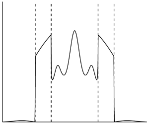

1. Introduction
This paper concerns decaying homogeneous turbulence in a rotating, stably stratified fluid with constant Brunt–Väisälä frequency and assumes that the rotation vector is parallel to gravity. The decay is due to viscous and diffusive effects which are detailed later. We refer the reader to the paper by Sagaut & Cambon (Reference Sagaut and Cambon2018) for a wide-ranging description of homogeneous turbulence, including, among other cases, rotation and stratification. In the present paper, one or other (or both) of the Rossby and Froude numbers is supposed to be small (weak turbulence), so nonlinearity is negligible over short enough time spans.
As discussed by Bartello (Reference Bartello1995) and Cambon (Reference Cambon2001), in the absence of nonlinearity and visco-diffusion, the flow consists of inertial-gravity wave modes, which oscillate in time, and a non-propagating (abbreviated to NP in what follows) mode which is steady. These modes form a complete set and so, even in the presence of nonlinearity and visco-diffusion, the flow can be expressed as a combination of modes. When weak nonlinearity and visco-diffusion are allowed for, the mode amplitudes evolve with time slowly compared to the oscillation period of the waves. The elucidation of the effects of this long-time evolution on the turbulence statistics in the presence of both rotation and stratification is the objective of this paper.
Weakness of turbulence has profound implications for the nonlinear dynamics, as indicated by wave-turbulence analysis, which is the usual approach for weak turbulence and has a long history (see e.g. Benney & Saffman Reference Benney and Saffman1966; Benney & Newell Reference Benney and Newell1969; Zakharov, Lvov & Falkovich Reference Zakharov, Lvov and Falkovich1992; Nazarenko Reference Nazarenko2011; Newell & Rumpf Reference Newell and Rumpf2011). According to that theory, nonlinear coupling between wave modes is dominated by resonances, non-resonant interactions being suppressed, which reduces the effectiveness of nonlinearity. More recently, studies have been undertaken (see e.g. Deng & Hani Reference Deng and Hani2021) which aim to place the theory on a rigorous mathematical basis.
Galtier (Reference Galtier2003) and Bellet et al. (Reference Bellet, Godeferd, Scott and Cambon2006) (henceforth referred to as [B]) used the wave-turbulence approach in the case of pure rotation, but we are unaware of any previous applications of wave-turbulence theory which allow for stratification. The difficulty is that wave-turbulence analysis requires that modes be dispersive, which is not true of the NP ones in the present problem. As a result, wave-turbulence analysis does not allow for the NP component of the flow, which must be analysed separately. In the special case  $N = 2\varOmega$, where N is the Brunt–Väisälä frequency and
 $\varOmega$ the rotation rate, the wave modes are also non-dispersive. To allow the application of wave-turbulence analysis to the wave component, we suppose that N is not too close to
 $2\varOmega$. This condition turns out to be also required by our treatment of the NP component.
Direct numerical simulation (DNS) of the governing equations has often been used (see e.g. Orszag & Patterson Reference Orszag and Patterson1972; Canuto et al. Reference Canuto, Hussaini, Quarteroni and Zang1988) to study homogeneous turbulence, and specifically in the present case of rotation and stratification by Coleman, Ferziger & Spalart (Reference Coleman, Ferziger and Spalart1992), Smith & Waleffe (Reference Smith and Waleffe2002) and Liechtenstein, Godeferd & Cambon (Reference Liechtenstein, Godeferd and Cambon2005). In this approach, the infinite flow is approximated as spatially periodic and is represented by Fourier series. However, DNS has difficulties when applied to the present problem if the turbulence is weak. This is because the intervention of nonlinearity requires evolution over many wave periods (according to wave-turbulence theory, the ratio of a typical wave period to the nonlinear time scale behaves as the square of the small parameter characterising the weakness of turbulence). The time step must be small compared with the wave period to resolve the associated oscillations, hence very many steps are needed before nonlinearity intervenes. Furthermore, the Fourier coefficients develop rapid oscillations in spectral space at large times, oscillations which need to be resolved numerically. This requires spatial periods considerably larger than the size of the large scales, otherwise numerical precision is degraded; the weaker the turbulence, the larger the required spatial periods. All of this means that the correct treatment by DNS of weak turbulence places considerable demands on computing time and memory requirements, demands which increase as the turbulence becomes weaker. With this in mind, the analytical and numerical methods developed here directly address the asymptotic limit of weak turbulence.
The spectral closure model EDQNM (eddy-damped, quasi-normal, Markovian) has also been used to study purely stratified and purely rotating turbulence (see Cambon & Jacquin Reference Cambon and Jacquin1989; Godeferd & Cambon Reference Godeferd and Cambon1994; Cambon, Mansour & Godeferd Reference Cambon, Mansour and Godeferd1997; Godeferd & Staquet Reference Godeferd and Staquet2003). EDQNM was introduced by Orszag (Reference Orszag1970) for homogeneous, isotropic turbulence and later extended to other cases in which there are dynamical mechanisms, such as stratification or rotation, which render the turbulence anisotropic, even if it is initially isotropic. For the case of pure rotation, the close relationship of EDQNM and wave-turbulence theory is one of the principal subjects of [B], where it is shown that the weak-turbulence limit of a particular version of EDQNM (EDQNM 3) gives the wave-turbulence equations for the spectra. It should, however, be recognised that models like EDQNM are based on ad hoc hypotheses, such as eddy-damping and quasi-normality, whereas wave-turbulence theory follows from detailed asymptotic analysis of weak turbulence (given in Appendix B for the present case), analysis which justifies closure in that limit.
The paper is organised as follows. Section 2 concerns the governing equations of the flow, their Fourier transforms, the definition of the modes, the results of modal projection (i.e. the mode amplitudes) and the mode-amplitude evolution equations. It also recognises the random nature of turbulent flow and, using ensemble averaging, defines a spectral matrix, denoted A, whose diagonal elements represent the energy distribution in spectral space of the different modes and whose off-diagonal elements express correlations between modes and are less important.
Section 3 introduces the assumption of weak turbulence and presents analyses of the consequences for the NP and wave components of the flow. In § 3.1, the NP component is found to evolve independently of the wave one and a numerical method, closely related to classical DNS of homogeneous turbulence, is proposed. However, although the methods are related, the flow field is here projected onto the NP modes at each time step, which distinguishes the present approach from the classical one. Note that, because we apply DNS only to the NP component, which is non-oscillatory, the problems of the classical approach, discussed above, do not arise.
Section 3.2 and Appendix B derive wave-turbulence equations which describe the time evolution of the wave part of the spectral matrix. To avoid the seeming intractability which the presence of the NP component entails if it is of comparable or greater magnitude than the wave one, the derivation requires that the NP component be small compared with the wave one. The end result is a system of equations for the diagonal elements of the wave-component spectral matrix.
Finally, § 4 describes results of numerical calculations for both the NP component using DNS and the wave component using the wave-turbulence equations.
2. Formulation
Consider decaying, homogeneous turbulence in a rotating, stably stratified fluid having constant Brunt–Väisälä frequency, N, and rotation vector,  $\boldsymbol{\varOmega }$, which is supposed to be parallel to gravity. It is also supposed that N and
 $\varOmega = |\boldsymbol{\varOmega }|$ are not both zero. When
 $\varOmega \ne 0$, an axial direction is defined by the unit vector
 $\boldsymbol{e} = \boldsymbol{\varOmega }/\varOmega$. However, if
 $\varOmega = 0$,
 $\boldsymbol{e}$ is taken in the vertical direction. Henceforth, spatial coordinates, time and velocity are non-dimensionalised using L,
 ${({N^2} + 4{\varOmega ^2})^{ - 1/2}}$ and
 $L{({N^2} + 4{\varOmega ^2})^{1/2}}$, where L is a length scale characterising the initial turbulence.
Using a rotating frame of reference and Cartesian coordinates (which will often be taken such that  $\boldsymbol{e} = (0,0,1)$), as well as the summation convention, the non-dimensional Boussinesq equations of motion are
 \begin{gather}\frac{{\partial {u_i}}}{{\partial t}} + \mathord{\buildrel{\lower3pt\hbox{$\scriptscriptstyle\frown$}} \over \varOmega } {\varepsilon _{ijk}}{e_j}{u_k} + \mathord{\buildrel{\lower3pt\hbox{$\scriptscriptstyle\frown$}} \over N} \eta {e_i} + \frac{{\partial p}}{{\partial {x_i}}} ={-} \frac{\partial }{{\partial {x_j}}}({u_i}{u_j}) + {D_u}\frac{{{\partial ^2}{u_i}}}{{\partial {x_j}\partial {x_j}}},\end{gather}
 \begin{gather}\frac{{\partial {u_i}}}{{\partial {x_i}}} = 0,\end{gather}
 \begin{gather}\frac{{\partial \eta }}{{\partial t}} - \mathord{\buildrel{\lower3pt\hbox{$\scriptscriptstyle\frown$}} \over N} {e_i}{u_i} ={-} \frac{\partial }{{\partial {x_j}}}(\eta {u_j}) + {D_\eta }\frac{{{\partial ^2}\eta }}{{\partial {x_j}\partial {x_j}}},\end{gather}
where  ${\varepsilon _{ijk}}$ is the alternating tensor,
 $\mathord{\buildrel{\lower3pt\hbox{$\scriptscriptstyle\frown$}} \over \varOmega } = 2\varOmega {({N^2} + 4{\varOmega ^2})^{ - 1/2}}$ and
 $\mathord{\buildrel{\lower3pt\hbox{$\scriptscriptstyle\frown$}} \over N} = N{({N^2} + 4{\varOmega ^2})^{ - 1/2}}$. Furthermore,
 ${D_u} = \nu {({N^2} + 4{\varOmega ^2})^{ - 1/2}}{L^{ - 2}}$ and
 ${D_\eta } = \kappa {({N^2} + 4{\varOmega ^2})^{ - 1/2}}{L^{ - 2}}$, where
 $\nu$ is the kinematic viscosity and
 $\kappa$ the diffusivity associated with the buoyancy variable
 $\eta$. Note that since
 ${\mathord{\buildrel{\lower3pt\hbox{$\scriptscriptstyle\frown$}} \over N} ^2} + {\mathord{\buildrel{\lower3pt\hbox{$\scriptscriptstyle\frown$}} \over \varOmega } ^2} = 1$,
 $\mathord{\buildrel{\lower3pt\hbox{$\scriptscriptstyle\frown$}} \over N} = {({\beta ^2} + 1)^{ - 1/2}}$ and
 $\mathord{\buildrel{\lower3pt\hbox{$\scriptscriptstyle\frown$}} \over \varOmega } = \beta {({\beta ^2} + 1)^{ - 1/2}}$, where
 $\beta = \mathord{\buildrel{\lower3pt\hbox{$\scriptscriptstyle\frown$}} \over \varOmega } /\mathord{\buildrel{\lower3pt\hbox{$\scriptscriptstyle\frown$}} \over N} = 2\varOmega /N$. Thus, the non-dimensional governing equations, (2.1)–(2.3), only depend on the parameters
 $\beta$,
 ${D_u}$ and
 ${D_\eta }$. For simplicity's sake,
 $\mathord{\buildrel{\lower3pt\hbox{$\scriptscriptstyle\frown$}} \over \varOmega }$,
 $\mathord{\buildrel{\lower3pt\hbox{$\scriptscriptstyle\frown$}} \over N}$ are denoted
 $\varOmega$, N in what follows. Because we will only be working with non-dimensional quantities, this should not lead to confusion. Note that the right-hand sides of (2.1) and (2.3) express nonlinearity, viscosity and diffusion. The visco-diffusive terms dissipate energy. When
 $N = 0$ (pure rotation), (2.1) and (2.2) decouple from (2.3), so the velocity field can be studied independently of
 $\eta$, which becomes a passive scalar. In all other cases, there is coupling in both directions between (2.1) and (2.3).
2.1. Fourier transforms and modes
Defining the Fourier transforms
 \begin{gather}{\tilde{u}_i}(\boldsymbol{k}) = \frac{1}{{8{{\rm \pi} ^3}}}\int {{u_i}(\boldsymbol{x})\exp ( - \textrm{i}\boldsymbol{k}\boldsymbol{\cdot }\boldsymbol{x})\,{\textrm{d}^3}\boldsymbol{x}} ,\end{gather}
 \begin{gather}\tilde{\eta }(\boldsymbol{k}) = \frac{1}{{8{{\rm \pi} ^3}}}\int {\eta (\boldsymbol{x})\exp ( - \textrm{i}\boldsymbol{k}\boldsymbol{\cdot }\boldsymbol{x})\,{\textrm{d}^3}\boldsymbol{x}} ,\end{gather}
with similar definitions of  $\tilde{p}$,
 $\widetilde {{u_i}{u_j}}$ and
 $\widetilde {\eta {u_j}}$, (2.1)–(2.3) yield
 \begin{gather}\frac{{\partial {{\tilde{u}}_i}}}{{\partial t}} + \varOmega {\varepsilon _{ijk}}{e_j}{\tilde{u}_k} + N\tilde{\eta }{e_i} + \textrm{i}{k_i}\tilde{p} ={-} {\rm i}{k_j}\widetilde {{u_i}{u_j}} - {D_u}{k^2}{\tilde{u}_i},\end{gather}
 \begin{gather}{k_i}{\tilde{u}_i} = 0,\end{gather}
 \begin{gather}\frac{{\partial \tilde{\eta }}}{{\partial t}} - N{e_i}{\tilde{u}_i} ={-} \textrm{i}{k_j}\widetilde {\eta {u_j}} - {D_\eta }{k^2}\tilde{\eta },\end{gather}
where  $k = |\boldsymbol{k}|$.
Appendix A examines the consequences of (2.6)–(2.8). In the absence of nonlinearity and visco-diffusion, the right-hand sides of (2.6) and (2.8) are zero. There are then three linearly independent solutions, referred to as modes. These solutions have time dependence  $\exp ( - \textrm{i}s\omega (\boldsymbol{k})t)$, where s takes one of the three values
 $s = 0,\; \pm 1$,
 \begin{equation}\omega (\boldsymbol{k}) = \frac{{{{({N^2}k_ \bot ^2 + {\varOmega ^2}k_\parallel ^2)}^{1/2}}}}{k} = {({N^2}{\sin ^2}{\theta _{\boldsymbol{k}}} + {\varOmega ^2}{\cos ^2}{\theta _{\boldsymbol{k}}})^{1/2}},\end{equation}
 ${k_ \bot } = |\boldsymbol{k} \times \boldsymbol{e}|$ is the transverse wavenumber,
 ${k_\parallel } = \boldsymbol{k}\boldsymbol{\cdot }\boldsymbol{e}$ is the axial wavenumber, and
 $0 \le {\theta _{\boldsymbol{k}}} \le {\rm \pi}$ is the angle between
 $\boldsymbol{k}$ and
 $\boldsymbol{e}$. The modes with
 $s ={\pm} 1$ represent inertial-gravity waves, for which (2.9) is the dispersion relation, while that with
 $s = 0$ will be referred to as the non-propagating (NP) mode because, when regarded as a wave, it has zero group velocity. The modal solutions of (2.6)–(2.8) (with zero right-hand sides) are
 \begin{gather}{\tilde{u}_i} = v_i^{(s)}(\boldsymbol{k})\exp ( - \textrm{i}s\omega (\boldsymbol{k})t),\end{gather}
 \begin{gather}\tilde{\eta } = {\eta ^{(s)}}(\boldsymbol{k})\exp ( - \textrm{i}s\omega (\boldsymbol{k})t),\end{gather}
where
 \begin{equation}v_i^{(s)}(\boldsymbol{k}) = \sum\limits_{l = 1}^2 {u_s^{(l)}(\boldsymbol{k})e_i^{(l)}(\boldsymbol{k})} ,\end{equation}
 \begin{equation}{\boldsymbol{e}^{(1)}} = \frac{{\boldsymbol{k} \times \boldsymbol{e}}}{{{k_ \bot }}},\quad {\boldsymbol{e}^{(2)}} = \frac{{\boldsymbol{k} \times {\boldsymbol{e}^{(1)}}}}{k},\end{equation}
are unit vectors orthogonal to each other and to  $\boldsymbol{k}$,
 \begin{equation}\left( {\begin{array}{@{}c@{}} {u_s^{(1)}}\\ {u_s^{(2)}}\\ {{\eta^{(s)}}} \end{array}} \right) = \frac{1}{{{2^{1/2}}{{({N^2}k_ \bot ^2 + {\varOmega ^2}k_\parallel ^2)}^{1/2}}}}\left( {\begin{array}{@{}c@{}} { - \varOmega {k_\parallel }}\\ {{\rm i}s{{({N^2}k_ \bot^2 + {\varOmega^2}k_\parallel^2)}^{1/2}}}\\ {N{k_ \bot }} \end{array}} \right),\end{equation}
when  $s ={\pm} 1$ and
 \begin{equation}\left( {\begin{array}{@{}c@{}} {u_0^{(1)}}\\ {u_0^{(2)}}\\ {{\eta^{(0)}}} \end{array}} \right) = \textrm{i}\frac{1}{{{{({N^2}k_ \bot ^2 + {\varOmega ^2}k_\parallel ^2)}^{1/2}}}}\left( {\begin{array}{@{}c@{}} {N{k_ \bot }}\\ 0\\ {\varOmega {k_\parallel }} \end{array}} \right).\end{equation}
It follows from (2.12)–(2.15) and the definitions of  ${k_ \bot }$ and
 ${k_\parallel }$ that
 $v_i^{(s)}( - \boldsymbol{k}) = v_i^{{{( - s)}^\ast }}(\boldsymbol{k})$ and
 ${\eta ^{(s)}}( - \boldsymbol{k}) = {\eta ^{{{( - s)}^\ast }}}(\boldsymbol{k})$, where * denotes complex conjugation. Note the orthonormality relation
 \begin{equation}\sum\limits_{l = 1}^2 {u_s^{{{(l)}^\ast }}u_{s^{\prime}}^{(l)}} + {\eta ^{{{(s)}^\ast }}}{\eta ^{(s^{\prime})}} = {\delta _{ss^{\prime}}},\end{equation}
where  ${\delta _{ss^{\prime}}}$ is the Kronecker delta. Note also that the
 $s = 0$ modes, referred to as NP here, are often described in the geophysical literature as ‘vortical modes’ or ‘potential vorticity (PV) modes’.
2.2. Mode-amplitude equation
The modes form a complete set for  ${\tilde{u}_i}$,
 $\tilde{\eta }$ satisfying (2.7). Thus,
 \begin{gather}{\tilde{u}_i} = \sum\limits_{s = 0, \pm 1} {{b_s}(\boldsymbol{k},t)v_i^{(s)}(\boldsymbol{k})} ,\end{gather}
 \begin{gather}\tilde{\eta } = \sum\limits_{s = 0, \pm 1} {{b_s}(\boldsymbol{k},t){\eta ^{(s)}}(\boldsymbol{k})} ,\end{gather}
where, as shown in Appendix A, the modal coefficients evolve according to
 \begin{equation}\frac{{\partial {b_s}}}{{\partial t}} + \textrm{i}s\omega {b_s} ={-} \textrm{i}{k_j}(v_i^{{{(s)}^\ast }}\widetilde {{u_i}{u_j}} + {\eta ^{{{(s)}^\ast }}}\widetilde {\eta {u_j}}) - \sum\limits_{\hat{s} = 0, \pm 1} {{D_{s\hat{s}}}{b_{\hat{s}}}} ,\end{equation}
in which
 \begin{equation}{D_{s\hat{s}}}(\boldsymbol{k}) = {k^2}\left( {{D_u}\sum\limits_{l = 1}^2 {u_s^{{{(l)}^\ast }}(\boldsymbol{k})u_{\hat{s}}^{(l)}(\boldsymbol{k})} + {D_\eta }{\eta^{{{(s)}^\ast }}}(\boldsymbol{k}){\eta^{(\hat{s})}}(\boldsymbol{k})} \right)\end{equation}
is a Hermitian, positive definite matrix expressing viscosity and diffusion. Real  ${u_i}$ and
 $\eta$ requires that
 ${\tilde{u}_i}( - \boldsymbol{k}) = \tilde{u}_i^\ast (\boldsymbol{k})$ and
 $\tilde{\eta }( - \boldsymbol{k}) = {\tilde{\eta }^\ast }(\boldsymbol{k})$, conditions which, according to (2.17), (2.18),
 $v_i^{(s)}( - \boldsymbol{k}) = v_i^{{{( - s)}^\ast }}(\boldsymbol{k})$ and
 ${\eta ^{(s)}}( - \boldsymbol{k}) = {\eta ^{{{( - s)}^\ast }}}(\boldsymbol{k})$, are met provided
 ${b_s}( - \boldsymbol{k}) = b_{ - s}^\ast (\boldsymbol{k})$.
Using (2.17), (2.18), and the inverse transforms of (2.4) and (2.5), the total flow can be expressed as the sum of wave and NP components:
 \begin{equation}{u_i} = u_i^W + u_i^{NP},\quad \eta = {\eta ^W} + {\eta ^{NP}},\end{equation}
where
 \begin{gather}u_i^W = \sum\limits_{s ={\pm} 1} {\int {{b_s}(\boldsymbol{k})v_i^{(s )}(\boldsymbol{k})\exp (\textrm{i}\boldsymbol{k}\boldsymbol{\cdot }\boldsymbol{x})\,{\textrm{d}^3}\boldsymbol{k}} } ,\end{gather}
 \begin{gather}{\eta ^W} = \sum\limits_{s ={\pm} 1} {\int {{b_s}(\boldsymbol{k}){\eta ^{(s)}}(\boldsymbol{k})\exp (\textrm{i}\boldsymbol{k}\boldsymbol{\cdot }\boldsymbol{x})\,{\textrm{d}^3}\boldsymbol{k}} } ,\end{gather}
 \begin{gather}u_i^{NP} = \int {{b_0}(\boldsymbol{k})v_i^{(0)}(\boldsymbol{k})\exp (\textrm{i}\boldsymbol{k}\boldsymbol{\cdot }\boldsymbol{x})\,{\textrm{d}^3}\boldsymbol{k}} ,\end{gather}
 \begin{gather}{\eta ^{NP}} = \int {{b_0}(\boldsymbol{k}){\eta ^{(0)}}(\boldsymbol{k})\exp (\textrm{i}\boldsymbol{k}\boldsymbol{\cdot }\boldsymbol{x})\,{\textrm{d}^3}\boldsymbol{k}} .\end{gather}
Given  ${b_s}( - \boldsymbol{k}) = b_{ - s}^\ast (\boldsymbol{k})$,
 $v_i^{(s)}( - \boldsymbol{k}) = v_i^{{{( - s)}^\ast }}(\boldsymbol{k})$ and
 ${\eta ^{(s)}}( - \boldsymbol{k}) = {\eta ^{{{( - s)}^\ast }}}(\boldsymbol{k})$, both components are real, the
 $s ={\pm} 1$ contributions to the wave component being complex conjugates.
If nonlinearity, viscosity and diffusion were neglected, the solution of (2.19) would have the expected modal form  ${b_s} \propto \exp ( - \textrm{i}s\omega t)$. The resulting oscillations of
 ${b_{ {\pm} 1}}$ due to waves can be supressed by defining
 ${a_s} = {b_s}\exp (\textrm{i}s\omega t)$, which evolves according to
 \begin{equation}\frac{{\partial {a_s}}}{{\partial t}} ={-} \textrm{i}{k_j}(v_i^{{{(s)}^\ast }}\widetilde {{u_i}{u_j}} + {\eta ^{{{(s)}^\ast }}}\widetilde {\eta {u_j}})\exp (\textrm{i}s\omega t) - \sum\limits_{\hat{s} = 0, \pm 1} {{D_{s\hat{s}}}\exp (\textrm{i}(s - \hat{s})\omega t){a_{\hat{s}}}} .\end{equation}
In the absence of nonlinearity and visco-diffusion, the mode amplitudes  ${a_s}$ are time-independent, whereas, when we later specialise to weak turbulence and small visco-diffusion, they evolve slowly with time. Here,
 ${b_s}( - \boldsymbol{k}) = b_{ - s}^\ast (\boldsymbol{k})$ and the definition of
 ${a_s}$ imply
 ${a_s}( - \boldsymbol{k}) = a_{ - s}^\ast (\boldsymbol{k})$.
As shown in Appendix A, the nonlinear term in (2.26) can be expressed as
 \begin{align}& -\!
\textrm{i}{k_j}(v_i^{{{(s)}^\ast }}\widetilde {{u_i}{u_j}}
+ {\eta ^{{{(s)}^\ast }}}\widetilde {\eta {u_j}})\exp
(\textrm{i}s\omega t)\nonumber\\ & \quad = \sum\limits_{{s_p},{s_q}
= 0, \pm 1} {\int {N_{s{s_p}{s_q}}^\ast
(\boldsymbol{k},\boldsymbol{p})a_{{s_p}}^\ast
(\kern1pt \boldsymbol{p})a_{{s_q}}^\ast ( - \boldsymbol{k} -
\boldsymbol{p})\exp
(\textrm{i}{F_{s{s_p}{s_q}}}(\boldsymbol{k},\boldsymbol{p})t)\,{\textrm{d}^3}\boldsymbol{p}}
},\end{align}
where
 \begin{equation}{N_{s{s_p}{s_q}}}(\boldsymbol{k},\boldsymbol{p}) = \textrm{i}{k_j}v_j^{({s_q})}( - \boldsymbol{k} - \boldsymbol{p})(v_i^{(s)}(\boldsymbol{k})v_i^{({s_p})}(\kern1pt \boldsymbol{p}) + {\eta ^{(s)}}(\boldsymbol{k}){\eta ^{({s_p})}}(\kern1pt \boldsymbol{p}))\end{equation}
represents nonlinear coupling between modes and
 \begin{equation}{F_{s{s_p}{s_q}}}(\boldsymbol{k},\boldsymbol{p}) = s\omega (\boldsymbol{k}) + {s_p}\omega (\kern1pt \boldsymbol{p}) + {s_q}\omega ( - \boldsymbol{k} - \boldsymbol{p}).\end{equation}
A symmetrised version of (2.27), namely
 \begin{align} & -\!
\textrm{i}{k_j}(v_i^{{{(s)}^\ast }}\widetilde {{u_i}{u_j}}
+ {\eta ^{{{(s)}^\ast }}}\widetilde {\eta {u_j}})\exp
(\textrm{i}s\omega t)\nonumber\\ & \quad = \sum\limits_{{s_p},{s_q}
= 0, \pm 1} {\int {M_{s{s_p}{s_q}}^\ast
(\boldsymbol{k},\boldsymbol{p})a_{{s_p}}^\ast
(\kern1pt \boldsymbol{p})a_{{s_q}}^\ast ( - \boldsymbol{k} -
\boldsymbol{p})\exp
(\textrm{i}{F_{s{s_p}{s_q}}}(\boldsymbol{k},\boldsymbol{p})t)\,{\textrm{d}^3}\boldsymbol{p}}
},\end{align}
where
 \begin{equation}{M_{s{s_p}{s_q}}}(\boldsymbol{k},\boldsymbol{p}) = {\textstyle{1 \over 2}}({N_{s{s_p}{s_q}}}(\boldsymbol{k},\boldsymbol{p}) + {N_{s{s_q}{s_p}}}(\boldsymbol{k}, - \boldsymbol{k} - \boldsymbol{p}))\end{equation}
is also derived in Appendix A. Using either (2.27) or (2.30), (2.26) provides an evolution equation for  ${a_s}$. Both versions are employed in what follows. Note the symmetries
 ${M_{s{s_p}{s_q}}}(\boldsymbol{k}, - \boldsymbol{k} - \boldsymbol{p}) = {M_{s{s_q}{s_p}}}(\boldsymbol{k},\boldsymbol{p})$ and
 ${F_{s{s_p}{s_q}}}(\boldsymbol{k}, - \boldsymbol{k} - \boldsymbol{p}) = {F_{s{s_q}{s_p}}}(\boldsymbol{k},\boldsymbol{p})$. Note also that the wave vectors
 $\boldsymbol{p}$ and
 $\boldsymbol{q} ={-} \boldsymbol{k} - \boldsymbol{p}$, which appear in (2.27) and (2.30), satisfy the usual condition,
 $\boldsymbol{k} + \boldsymbol{p} + \boldsymbol{q} = 0$, for formation of a triad with
 $\boldsymbol{k}$.
2.3. The spectral matrix and energy
Here and henceforth, the random nature of turbulent flow is recognised and ensemble averaging introduced. The flow is assumed statistically homogeneous, i.e. its statistical properties are the same at all spatial locations, in particular, any one-point average is independent of position. Averaging (2.1) and (2.3) eliminates the nonlinear, pressure and visco-diffusive terms, while the average of (2.2) is automatically satisfied. We have in mind that there is no mean flow, i.e.  $\overline {{u_i}} = 0$, where the overbar denotes ensemble averaging, hence the average of (2.1) gives
 $\bar{\eta } = 0$. Here,
 $\overline {{u_i}} = \bar{\eta } = 0$ leads to
 $\overline {{a_s}} = \overline {{b_s}} = 0$, while (2.22)–(2.25) imply that the wave and NP components are both of zero mean. Those components also inherit the statistical homogeneity of the total flow.
The ensemble-averaged, non-dimensional energy density in physical space is the sum of kinetic and potential energies:
 \begin{equation}\underbrace{{{\textstyle{1 \over 2}}\overline {{u_i}{u_i}} }}_{{Kinetic}} + \underbrace{{{\textstyle{1 \over 2}}\overline {{\eta ^2}} }}_{{Potential}}.\end{equation}
Given statistical homogeneity,
 \begin{equation}\overline {\tilde{u}_i^\ast (\boldsymbol{k}){{\tilde{u}}_i}(\boldsymbol{k^{\prime}})} = {\varPhi _u}(\boldsymbol{k})\delta (\boldsymbol{k} - \boldsymbol{k^{\prime}}),\quad \overline {{{\tilde{\eta }}^\ast }(\boldsymbol{k})\tilde{\eta }(\boldsymbol{k^{\prime}})} = {\varPhi _\eta }(\boldsymbol{k})\delta (\boldsymbol{k} - \boldsymbol{k^{\prime}}),\end{equation}
in which  $\delta$ represents the Dirac function. Hence, using the inverse transform of (2.4),
 \begin{align}
\dfrac{1}{2}\overline {{u_i}{u_i}} &= \dfrac{1}{2}\int {\int
{\overline {\tilde{u}_i^\ast
(\boldsymbol{k}){{\tilde{u}}_i}(\boldsymbol{k^{\prime}})}
\exp (\textrm{i}(\boldsymbol{k^{\prime}} -
\boldsymbol{k})\boldsymbol{\cdot
}\boldsymbol{x})\,{\textrm{d}^3}\boldsymbol{k^{\prime}}}
\,{\textrm{d}^3}\boldsymbol{k}}\nonumber \\ &= \dfrac{1}{2}\int
{{\varPhi
_u}(\boldsymbol{k})\,{\textrm{d}^3}\boldsymbol{k}} ,
\end{align}
which indicates that the kinetic-energy density in spectral space is  ${e_K}(\boldsymbol{k}) = {\varPhi _u}/2$. Similarly, the potential-energy density in spectral space is
 ${e_P}(\boldsymbol{k}) = {\varPhi _\eta }/2$.
Again, using statistical homogeneity,
 \begin{equation}\overline {a_s^\ast (\boldsymbol{k}){a_{s^{\prime}}}(\boldsymbol{k^{\prime}})} = {A_{ss^{\prime}}}(\boldsymbol{k})\delta (\boldsymbol{k} - \boldsymbol{k^{\prime}}),\end{equation}
where  ${A_{ss^{\prime}}}$ is the spectral matrix and s,
 $s^{\prime}$ run over the values
 $- 1$,
 $0$ and
 $+ 1$;
 ${A_{ss^{\prime}}}$ is Hermitian and positive semi-definite. In particular, the diagonal elements of
 ${A_{ss^{\prime}}}$ are real and non-negative. Also, given
 ${a_s}( - \boldsymbol{k}) = a_{ - s}^\ast (\boldsymbol{k})$,
 ${A_{ss^{\prime}}}( - \boldsymbol{k}) = {A_{ - s^{\prime}, - s}}(\boldsymbol{k})$. Using (2.12), (2.17), (2.18), (2.35),
 $e_i^{(l)}(\boldsymbol{k})e_i^{(l^{\prime})}(\boldsymbol{k}) = {\delta _{ll^{\prime}}}$ and
 ${b_s} = {a_s}\exp ( - \textrm{i}s\omega t)$ to evaluate the averages in (2.33),
 \begin{gather}{e_K} = \frac{1}{2}\sum\limits_{s,s^{\prime} = 0, \pm 1} {{A_{ss^{\prime}}}(u_s^{{{(1)}^\ast }}u_{s^{\prime}}^{(1)} + u_s^{{{(2)}^\ast }}u_{s^{\prime}}^{(2)})} \exp (\textrm{i}(s - s^{\prime})\omega t),\end{gather}
 \begin{gather}{e_P} = \frac{1}{2}\sum\limits_{s,s^{\prime} = 0, \pm 1} {{A_{ss^{\prime}}}{\eta ^{{{(s)}^\ast }}}{\eta ^{(s^{\prime})}}\exp (\textrm{i}(s - s^{\prime})\omega t)} .\end{gather}
Note that (2.16) implies
 \begin{equation}e = {e_K} + {e_P} = \frac{1}{2}\sum\limits_{s = 0, \pm 1} {{A_{ss}}} ,\end{equation}
for the total energy density. Thus,  ${A_{ss^{\prime}}}$ determines the energy densities in spectral space, but it contains considerably more statistical information than that: any second-order, two-point moment involving
 ${u_i}$ and
 $\eta$ can be obtained knowing
 ${A_{ss^{\prime}}}$.
The diagonal elements of  ${A_{ss^{\prime}}}$ can be interpreted as the energy densities of the different modes and will often be referred to as spectra, whereas the off-diagonal ones represent correlations between modes. As usual, it can be shown that the nonlinear term in (2.26) conserves the total energy, which decays due to visco-diffusion according to
 \begin{equation}\frac{\textrm{d}}{{\textrm{d}t}}\int {e(\boldsymbol{k})\,{\textrm{d}^3}\boldsymbol{k}} ={-} \textrm{Re} \biggl( {\int {\sum\limits_{s,\hat{s} = 0, \pm 1} {D_{s\hat{s}}^\ast (\boldsymbol{k})\exp (\textrm{i}(\hat{s} - s)\omega (\boldsymbol{k})t){A_{\hat{s}s}}(\boldsymbol{k})} \,{\textrm{d}^3}\boldsymbol{k}} } \biggr).\end{equation}
Finally, a spherically averaged spectrum,  $E(k)$, can be defined by averaging
 $e(\boldsymbol{k})$ over the sphere
 $|\boldsymbol{k}|= k$, then multiplying by
 $4{\rm \pi} {k^2}$. When integrated over k,
 $E(k)$ gives the total energy. It represents the energy distribution in spectral space, without regard for anisotropy. Obviously,
 $E(k)$ contains less information than
 $e(\boldsymbol{k})$.
The energy density in spectral space, given by (2.38), can be split into wave and NP contributions as  $e = {e_W} + {e_{NP}}$, where
 \begin{equation}{e_W} = \frac{1}{2}\sum\limits_{s ={\pm} 1} {{A_{ss}}} ,\quad {e_{NP}} = \frac{1}{2}{A_{00}}.\end{equation}
The spherically averaged spectrum can also be split into wave and NP contributions as  $E = {E_W} + {E_{NP}}$, where
 ${E_W}$ and
 ${E_{NP}}$ are obtained from
 ${e_W}$ and
 ${e_{NP}}$ in the same way that E follows from e.
3. Weak turbulence
From here on, we suppose that  ${u_i}$ and
 $\eta$ are small. This means that linear theory applies over time intervals of
 $O(1)$. Small nonlinearity can nonetheless have significant cumulative effects over longer time scales, effects whose quantification is the aim of this article. However, this requires sufficiently small visco-diffusive dissipation, otherwise it will kill the turbulence before nonlinearity can intervene. Given weak turbulence and small visco-diffusion, we consider large t.
As discussed in the introduction, wave-turbulence analysis is the usual approach to describe weak turbulence in the presence of waves. However, it requires that the waves be dispersive. Since the frequency of the NP mode is zero, it has zero group velocity and hence is non-dispersive, which rules out direct application of the wave-turbulence approach to the flow as a whole. Furthermore, when  $\varOmega = N$,
 $\omega (\boldsymbol{k}) = \varOmega = N$ is constant, in which case the wave mode is also non-dispersive, while if
 $|\varOmega - N|$ is small, but non-zero, it is only weakly dispersive. Many of the steps in the analysis require
 $|\varOmega - N|\gg {t^{ - 1}}$, an assumption which is made from here on. This assumption opens the way for wave-turbulence theory of the wave modes, but care is still needed because of the non-dispersive character of the NP mode. Wave-turbulence analysis cannot be applied to the NP component of the flow, which is analysed separately.
The weakness of turbulence is expressed by small parameters,  $\varepsilon$ and
 ${\varepsilon _{NP}}$, which respectively measure the amplitudes of the wave and NP components. The parameters need not have the same order of magnitude. Indeed, to close the system of equations for the wave component, we will later suppose that
 ${\varepsilon _{NP}}$ is small compared with
 $\varepsilon$.
In the following analysis, we suppose that neither N nor  $\varOmega$ are zero, which excludes pure rotation or stratification. This avoids having to deal with special cases where, rather than being strictly positive,
 $\omega (\boldsymbol{k})$ is zero for particular values of
 ${\theta _{\boldsymbol{k}}}$ (
 ${\theta _{\boldsymbol{k}}} = {\rm \pi}/2$ when
 $N = 0$,
 ${\theta _{\boldsymbol{k}}} = 0,{\rm \pi}$ when
 $\varOmega = 0$). We will nonetheless later give results for the limiting cases
 $N = 0$ and
 $\varOmega = 0$.
3.1. Evolution of the NP component
Applying (2.26) with  $s = 0$,
 \begin{equation}\frac{{\partial {a_0}}}{{\partial t}} ={-} \textrm{i}{k_j}(v_i^{{{(0)}^\ast }}\widetilde {{u_i}{u_j}} + {\eta ^{{{(0)}^\ast }}}\widetilde {\eta {u_j}}) - \sum\limits_{\hat{s} = 0, \pm 1} {{D_{0\hat{s}}}\exp ( - \textrm{i}\hat{s}\omega (\boldsymbol{k})t){a_{\hat{s}}}} .\end{equation}
Using the decomposition into wave and NP components, (2.21),
 \begin{gather}{u_i}{u_j} = \underbrace{{u_i^{NP}u_j^{NP}}}_{{NP\textrm{-}NP}} + \underbrace{{u_i^Wu_j^W}}_{{wave \textrm{-} wave}} + \underbrace{{u_i^Wu_j^{NP} + u_i^{NP}u_j^W}}_{{wave \textrm{-} NP}},\end{gather}
 \begin{gather}\eta {u_j} = \underbrace{{{\eta ^{NP}}u_j^{NP}}}_{{NP \textrm{-} NP}} + \underbrace{{{\eta ^W}u_j^W}}_{{wave \textrm{-} wave}} + \underbrace{{{\eta ^W}u_j^{NP} + {\eta ^{NP}}u_j^W}}_{{wave \textrm{-} NP}}.\end{gather}
Thus, there are three contributions to the nonlinear term in (3.1): NP-NP, wave-wave and wave-NP.
The right-hand side of (3.1) represents nonlinearity and visco-diffusion. As discussed above, both are negligible over time spans of  $O(1)$, but can have significant cumulative effects over the longer time scales considered here. The wave component has oscillations of periods
 $O(1)$, whereas the NP one is steady on such time scales. Thus, the wave-NP contributions to (3.2) and (3.3) are oscillatory and their cumulative effect following evolution according to (3.1) remains small and is neglected. Furthermore, the
 $\hat{s} ={\pm} 1$ contributions to the visco-diffusive term are also oscillatory and hence negligible. Thus, we obtain the approximation
 \begin{equation}\frac{{\partial {a_0}}}{{\partial t}} + {D_{00}}{a_0} ={-} \textrm{i}{k_j}(v_i^{{{(0)}^\ast }}\widetilde {u_i^{NP}u_j^{NP}} + {\eta ^{{{(0)}^\ast }}}\widetilde {{\eta ^{NP}}u_j^{NP}}) + f,\end{equation}
where the first term on the right-hand side expresses nonlinear interactions between NP modes and
 \begin{equation}f(\boldsymbol{k},t) ={-} \textrm{i}{k_j}(v_i^{{{(0)}^\ast }}\widetilde {u_i^Wu_j^W} + {\eta ^{{{(0)}^\ast }}}\widetilde {{\eta ^W}u_j^W})\end{equation}
represents forcing of the NP mode by the wave component.
Following the procedure which led to (2.30), but without the NP contributions,
 \begin{equation}f(\boldsymbol{k},t) = \sum\limits_{{s_p},{s_q} ={\pm} 1} {\int {M_{0{s_p}{s_q}}^\ast (\boldsymbol{k},\boldsymbol{p})a_{{s_p}}^\ast (\kern1pt \boldsymbol{p})a_{{s_q}}^\ast ( - \boldsymbol{k} - \boldsymbol{p})\exp (\textrm{i}{F_{0{s_p}{s_q}}}(\boldsymbol{k},\boldsymbol{p})t)\,{\textrm{d}^3}\boldsymbol{p}} } .\end{equation}
Using (2.29),  ${F_{0{s_p}{s_q}}}(\boldsymbol{k},\boldsymbol{p}) = {s_p}\omega (\kern1pt \boldsymbol{p}) + {s_q}\omega ( - \boldsymbol{k} - \boldsymbol{p})$. Since
 $\omega > 0$, the exponential in (3.6) is oscillatory when
 ${s_p} = {s_q}$ and such terms are therefore neglected. Assuming
 $|\varOmega - N|t$ is large, if
 ${s_p} ={-} {s_q}$, the exponential is oscillatory with period
 $O(1)$ for
 $\boldsymbol{p}$ away from the surface
 $\omega (\kern1pt \boldsymbol{p}) = \omega ( - \boldsymbol{k} - \boldsymbol{p})$. Neglecting such
 $\boldsymbol{p}$, we focus on
 $\boldsymbol{p}$ close to the surface, where the exponential oscillates slowly, potentially allowing significant cumulative effects at long times. However, although we have been unable to show it analytically, numerical calculations with different values of
 $\beta \ne 1$,
 $\boldsymbol{k}$ and
 $\boldsymbol{p}$ show that
 ${M_{0,s, - s}}(\boldsymbol{k},\boldsymbol{p})$ is zero to IEEE double precision when
 $s \ne 0$ and
 $\omega (\kern1pt \boldsymbol{p}) = \omega ( - \boldsymbol{k} - \boldsymbol{p})$. Assuming this result, which is a priori far from obvious, is exactly true, slow oscillations are suppressed and we suppose the forcing term in (3.4) is negligible.
Recall from (2.40) that the energy density in spectral space can be split into wave and NP contributions and that the NP contribution is
 \begin{equation}{e_{NP}} = {\textstyle{1 \over 2}}{A_{00}}.\end{equation}
Appendix D (Supplementary material is available at https://doi.org/10.1017/jfm.2023.1046) shows that the first term on the right-hand side of (3.4), representing nonlinear interactions between NP modes, conserves the total energy of the NP component, which, neglecting the forcing term, decays due to visco-diffusive dissipation according to
 \begin{equation}\frac{\textrm{d}}{{\textrm{d}t}}\int {{e_{NP}}(\boldsymbol{k})\,{\textrm{d}^3}\boldsymbol{k}} ={-} 2\int {{D_{00}}(\boldsymbol{k}){e_{NP}}(\boldsymbol{k})\,{\textrm{d}^3}\boldsymbol{k}} .\end{equation}
Let  ${\varepsilon _{NP}}$ be a small parameter measuring the amplitude of the NP component, thus
 $\hat{u}_i^{NP} = u_i^{NP}/{\varepsilon _{NP}}$ and
 ${\hat{\eta }^{NP}} = {\eta ^{NP}}/{\varepsilon _{NP}}$ are
 $O(1)$. Equations (2.24) and (2.25) with
 ${b_0} = {a_0}$ give
 \begin{gather}\hat{u}_i^{NP}(\boldsymbol{x}) = \int {{{\hat{a}}_0}(\boldsymbol{k})v_i^{(0)}(\boldsymbol{k})\exp (\textrm{i}\boldsymbol{k}\boldsymbol{\cdot }\boldsymbol{x})\,{\textrm{d}^3}\boldsymbol{k}} ,\end{gather}
 \begin{gather}{\hat{\eta }^{NP}}(\boldsymbol{x}) = \int {{{\hat{a}}_0}(\boldsymbol{k}){\eta ^{(0)}}(\boldsymbol{k})\exp (\textrm{i}\boldsymbol{k}\boldsymbol{\cdot }\boldsymbol{x})\,{\textrm{d}^3}\boldsymbol{k}} ,\end{gather}
where  ${\hat{a}_0} = {a_0}/{\varepsilon _{NP}}$. Without the forcing term, (3.4) yields
 \begin{equation}\frac{{\partial {{\hat{a}}_0}}}{{\partial \hat{t}}} + {\hat{D}_{00}}{\hat{a}_0} ={-} \textrm{i}{k_j}(v_i^{{{(0)}^\ast }}\widetilde {\hat{u}_i^{NP}\hat{u}_j^{NP}} + {\eta ^{{{(0)}^\ast }}}\widetilde {{{\hat{\eta }}^{NP}}\hat{u}_j^{NP}}),\end{equation}
where  $\hat{t} = {\varepsilon _{NP}}t$ is time, scaled appropriately for evolution of the NP component, and
 ${\hat{D}_{00}} = {D_{00}}/{\varepsilon _{NP}}$. Thus, the NP component evolves according to (3.9)–(3.11). Assuming visco-diffusion is sufficiently small that it does not kill the turbulence before nonlinearity intervenes, the time scale for NP evolution is
 $O(\varepsilon _{NP}^{ - 1})$. This time scale is generally distinct from that of
 $O({\varepsilon ^{ - 2}})$, which, as we will see later, characterises the wave component according to wave-turbulence theory.
Before going further, we should discuss the close relationship between the theory of the NP component described here and quasi-geostrophic (QG) theory (see Pedlosky Reference Pedlosky1987), which is one of the cornerstones in the study of atmospheric and oceanic flows since its development by Charney (Reference Charney1948, Reference Charney1971). NP modes represent geostrophic flows (i.e. the Coriolis and pressure-gradient terms in the horizontal momentum equation balance) and the NP component of the real flow can be regarded as its mathematical projection onto such idealised flows. With this in mind, it can be shown that, for the present problem, (3.9)–(3.11) are equivalent to the three-dimensional QG approximation, thus providing support for the present approach.
Embid & Madja (Reference Embid and Madja1998) give asymptotic analysis of (2.1)–(2.3) for small Froude number and consider two cases. In the first, the Rossby number is small, and they conclude that the flow consists of oscillatory waves and a slowly varying component which evolves according to the quasi-geostrophic approximation, in agreement with the present results. In the second case, the Rossby number is of order one, corresponding to a small value of  $\beta$. This makes
 $N\sim 1$ and
 $\varOmega \sim \beta$, thus the wave frequency, (2.9), is small for small
 ${\theta _{\boldsymbol{k}}}$, i.e. waves having wave vectors near the axis
 ${k_ \bot } = 0$ are slowly varying. Given such modes, one might question the neglect of the wave-NP contribution to (3.1), which was based on oscillatory waves and led to (3.4). For Rossby numbers of order one, Embid and Majda supposed the slow, horizontal component of the flow to be the sum of two parts (see their (3.31)), one of which is the so-called VSHF (vertically sheared horizontal flow), which is independent of
 ${x_1}$ and
 ${x_2}$, and can be considered as a combination of wave modes with
 ${k_ \bot } = 0$. They derived evolution equations for both parts of the flow (see their (3.33) and (3.34)) and found that the VSHF component entered into the equation for the other part. This corresponds to coupling of the wave and NP components, and neglect of the wave-NP contribution to (3.1) does not capture such coupling. However, the assumed form of the flow places significant wave energy precisely on the axis,
 ${k_ \bot } = 0$, which is not the situation we have in mind. Instead, we envisage a continuous distribution of energy over wave vectors. In that case, we believe that the neglect of the wave-NP contribution to (3.1) is justified at small
 $\beta$ by the smallness of the region in
 ${\theta _{\boldsymbol{k}}}$ for which the wave frequency is small. Whether or not the flow will eventually evolve towards a state close to that assumed by Embid and Majda is unclear.
Equation (3.11) is integrated numerically. Equations (3.9) and (3.10) yield  $\hat{u}_i^{NP}(\boldsymbol{x})$ and
 ${\hat{\eta }^{NP}}(\boldsymbol{x})$ as inverse Fourier transforms. Then,
 $\hat{u}_i^{NP}\hat{u}_j^{NP}$ and
 ${\hat{\eta }^{NP}}\hat{u}_j^{NP}$ can be calculated in physical space, while forward transformation gives
 $\widetilde {\hat{u}_i^{NP}\hat{u}_j^{NP}}$ and
 $\widetilde {{{\hat{\eta }}^{NP}}\hat{u}_j^{NP}}$ for use in (3.11). This resembles classical DNS of homogeneous turbulence and the numerical method employed here is based on that approach and is described in Appendix F (Supplementary material). However, as noted in the introduction, it differs significantly from classical DNS because of the projection onto the NP modes at each time step, a projection which is implicit in (3.11).
3.2. Evolution of the wave component
Terms in the sum of (2.26) with  $\hat{s} \ne s$ are oscillatory and hence negligible for the long-time evolution of
 ${a_s}$. Adopting this approximation and using (2.30), (2.26) becomes
 \begin{align} &
\dfrac{{\partial {a_s}(\boldsymbol{k})}}{{\partial t}} +
{D_{ss}}(\boldsymbol{k}){a_s}(\boldsymbol{k})\nonumber\\ & \quad =
\sum\limits_{{s_p},{s_q} = 0, \pm 1} {\int
{M_{s{s_p}{s_q}}^\ast
(\boldsymbol{k},\boldsymbol{p})a_{{s_p}}^\ast
(\kern1pt \boldsymbol{p})a_{{s_q}}^\ast ( - \boldsymbol{k} -
\boldsymbol{p})\exp
(\textrm{i}{F_{s{s_p}{s_q}}}(\boldsymbol{k},\boldsymbol{p})t)\,{\textrm{d}^3}\boldsymbol{p}}
} . \end{align}
Appendix B describes wave-turbulence analysis based on (3.12). It is assumed that  $|\varOmega - N|t$ is large. Furthermore, to obtain closed equations for the wave component, it is supposed that the amplitude of the NP component is small compared with that of the wave component. The result is (B52) for evolution of the wave elements (
 ${A_{ss^{\prime}}}$,
 $s,s^{\prime} \ne 0$) of the spectral matrix. Since the wave-component spectral energy density is given by the first of (2.40), the most interesting application of (B52) is
 $s^{\prime} = s$, hence (B53), which involves Cauchy principal-value integrals. However, somewhat remarkably, it is found that the sum of such contributions is zero, as is the sum of
 ${s_q} = 0$ contributions to the first term on the right-hand side of (B53). The final result is
 \begin{align} &
\dfrac{{\partial
{{\hat{A}}_{ss}}(\boldsymbol{k})}}{{\partial T}} +
2\hat{D}(\boldsymbol{k}){{\hat{A}}_{ss}}(\boldsymbol{k}) =
2{\rm \pi} \sum\limits_{{s_p},{s_q} ={\pm} 1}
{\int_{{S_{s{s_p}{s_q}}}(\boldsymbol{k})}
{\dfrac{{{{\hat{A}}_{{s_p}{s_p}}}(\kern1pt \boldsymbol{p})}}{{|{s_p}{\boldsymbol{c}_g}(\kern1pt \boldsymbol{p})
+ {s_q}{\boldsymbol{c}_g}(\boldsymbol{k} +
\boldsymbol{p})|}}} } \nonumber\\ & \quad\times ({\lambda
_{s{s_p}{s_q}}}(\boldsymbol{k},\boldsymbol{p}){{\hat{A}}_{{s_q}{s_q}}}(
- \boldsymbol{k} -\kern1pt\boldsymbol{p}) + \textrm{Re} ({\zeta
_{s{s_p}{s_q}}}(\boldsymbol{k},\boldsymbol{p})){{\hat{A}}_{ss}}(\boldsymbol{k}))\,{\textrm{d}^2}\boldsymbol{p},
\end{align}
for  $s \ne 0$, where
 $T = {\varepsilon ^2}t$ is time, scaled appropriately for evolution of the wave component,
 ${\hat{A}_{ss}} = {A_{ss}}/{\varepsilon ^2}$ are the
 $O(1)$ scaled wave spectra,
 $\hat{D} = D/{\varepsilon ^2}$,
 \begin{equation}D(\boldsymbol{k}) = {k^2}\frac{{{D_u}({N^2}k_ \bot ^2 + 2{\varOmega ^2}k_\parallel ^2) + {D_\eta }{N^2}k_ \bot ^2}}{{2({N^2}k_ \bot ^2 + {\varOmega ^2}k_\parallel ^2)}}\end{equation}
is the damping coefficient of wave modes (i.e.  ${D_{ss}}(\boldsymbol{k}) = D(\boldsymbol{k})$ for
 $s \ne 0$),
 \begin{equation}{\boldsymbol{c}_g}(\boldsymbol{k}) = {\nabla _{\boldsymbol{k}}}\omega (\boldsymbol{k})\end{equation}
gives the group velocity of the wave modes as  $s{\boldsymbol{c}_g}$,
 \begin{gather}{\lambda _{s{s_p}{s_q}}}(\boldsymbol{k},\boldsymbol{p}) = 2|{M_{s{s_p}{s_q}}}(\boldsymbol{k},\boldsymbol{p}){|^2},\end{gather}
 \begin{gather}{\zeta _{s{s_p}{s_q}}}(\boldsymbol{k},\boldsymbol{p}) = 4{M_{s{s_p}{s_q}}}(\boldsymbol{k},\boldsymbol{p})M_{{s_q}s{s_p}}^\ast ( - \boldsymbol{k} - \boldsymbol{p},\boldsymbol{k}),\end{gather}
and  ${S_{s{s_p}{s_q}}}(\boldsymbol{k})$ is the surface in
 $\boldsymbol{p}$-space defined by
 ${F_{s{s_p}{s_q}}}(\boldsymbol{k},\boldsymbol{p}) = 0$. As is apparent from (2.29), the surface
 ${S_{s{s_p}{s_q}}}(\boldsymbol{k})$ is such that
 $s\omega (\boldsymbol{k}) + {s_p}\omega (\kern1pt \boldsymbol{p}) + {s_q}\omega ( - \boldsymbol{k} - \boldsymbol{p}) = 0$. This condition represents triadic resonances, triadic since it involves three wave vectors,
 $\boldsymbol{k}$,
 $\boldsymbol{p}$ and
 $- \boldsymbol{k} - \boldsymbol{p}$ which sum to zero, and resonant because it says that the sum of modal frequencies is zero. For this reason,
 ${S_{s{s_p}{s_q}}}(\boldsymbol{k})$ will be referred to as the resonant surface. If there are no such resonances for given
 $\boldsymbol{k}$, s,
 ${s_p}$ and
 ${s_q}$ (i.e.
 ${F_{s{s_p}{s_q}}}(\boldsymbol{k},\boldsymbol{p}) = 0$ has no solutions in
 $\boldsymbol{p}$-space),
 ${S_{s{s_p}{s_q}}}(\boldsymbol{k})$ is the empty set and the surface integral in (3.13) should be interpreted as zero.
It is perhaps interesting to discuss (3.13) in the context of EDQNM. Eddy damping does not appear (for the case of pure rotation, it was shown in [B] that it vanishes in the limit of weak turbulence). Quasi-normality is a consequence of wave-turbulence analysis and is apparent in (3.13) via the products of spectra on the right-hand side which represent fourth-order spectral moments. The fact that, according to (3.13), the spectrum at time t evolves according to its values at the same instant justifies the final, Markovian, closure hypothesis of EDQNM. An important difference between wave-turbulence theory and EDQNM is that the nonlinear term in (3.13) is a surface integral over resonant triads, whereas it is a volume integral over all triads, including non-resonant ones, according to EDQNM. For the case of pure rotation, it was shown in [B] that the volume integral of EDQNM is dominated by resonant triads in the limit of weak turbulence, hence the wave-turbulence result is approached.
Appendix E (Supplementary material) analyses the energetics of the wave component based on (3.13). It is shown that the right-hand side of (3.13) conserves the total wave-component energy, which evolves according to
 \begin{equation}\frac{\textrm{d}}{{\textrm{d}t}}\int {{e_W}(\boldsymbol{k})\,{\textrm{d}^3}\boldsymbol{k}} ={-} 2\int {D(\boldsymbol{k}){e_W}(\boldsymbol{k})\,{\textrm{d}^3}\boldsymbol{k}} .\end{equation}
Taking the sum of (3.8) and (3.18),
 \begin{equation}\frac{\textrm{d}}{{\textrm{d}t}}\int {e(\boldsymbol{k})\,{\textrm{d}^3}\boldsymbol{k}} ={-} 2\int {({D_{00}}(\boldsymbol{k}){e_{NP}}(\boldsymbol{k}) + D(\boldsymbol{k}){e_W}(\boldsymbol{k}))\,{\textrm{d}^3}\boldsymbol{k}} .\end{equation}
This result may be compared with the exact energy equation (2.39). In the weak-turbulence limit considered here, terms in the sum of (2.39) with  $\hat{s} \ne s$ are oscillatory and hence negligible. Dropping these terms gives (3.19). Thus, as regards the total energy, the present approximations agree with the weak-turbulence limit of the exact result.
Appendix C concerns the existence of solutions of  ${F_{s{s_p}{s_q}}}(\boldsymbol{k},\boldsymbol{p}) = 0$, where s,
 ${s_p}$ and
 ${s_q}$ take one of the values
 ${\pm} 1$. It is shown that the resonant surface does not exist if
 $s = {s_p} = {s_q}$ or
 $1/2 \le \beta \le 2$ (a result in agreement with Smith & Waleffe (Reference Smith and Waleffe2002), § 6.1). Thus, when
 $1/2 \le \beta \le 2$, the right-hand side of (3.13) is zero according to the present theory. Nonlinear interactions between wave modes are then absent at the order to which we are working, suggesting the need to go to higher order. However, that lies beyond the scope of the present work. When
 $\beta < 1/2$ or
 $\beta > 2$, the resonant surface exists for
 ${s_p} = {s_q} \ne s$ provided
 \begin{equation}\omega (\boldsymbol{k}) > 2\min(\varOmega ,N),\end{equation}
and for  ${s_p} ={-} {s_q}$ when
 \begin{equation}\omega (\boldsymbol{k}) < |\varOmega - N|.\end{equation}
If  $\beta < 1/3$ or
 $\beta > 3$, one or other of (3.20) or (3.21) is satisfied for all
 $\boldsymbol{k}$, hence resonant surfaces can always be found for such values of
 $\beta$. However, when
 $1/3 < \beta < 1/2$ or
 $2 < \beta < 3$, there are directions of
 $\boldsymbol{k}$ for which neither (3.20) nor (3.21) hold, hence no resonant surfaces. Such wave vectors are decoupled from all others according to (3.13), which predicts that these modes simply decay under visco-diffusive dissipation. Thus, spectral space can be divided into two regions. In the first (referred to as A), either (3.20) or (3.21) applies and there is nonlinear coupling between wave modes within that region. In the second (B), such coupling is absent. This distinction expresses different dynamics for the two types of modes, but is only significant for
 $1/3 < \beta < 1/2$ or
 $2 < \beta < 3$, otherwise all modes are of type A. Note that the extent of the region in which inter-mode coupling occurs shrinks down to zero as either
 $\beta \nearrow 1/2$ or
 $\beta \searrow 2$, which is the way in which nonlinearity of the order considered here disappears as those boundaries are approached.
Consider a wave vector for which there is one or more resonant surfaces and suppose visco-diffusive dissipation small enough  $(D \le O({\varepsilon ^2}))$ that it does not kill the wave component before nonlinearity intervenes, the time scale for evolution of the wave component implied by (3.13) is
 $t\sim O({\varepsilon ^{ - 2}})$, the usual one for wave turbulence. If there is no resonant surface, we expect the nonlinear evolution time to be longer. As noted earlier, the time scales for evolution of the wave and NP components are generally distinct.
Appendix G (Supplementary material) describes the numerical method used to solve (3.13) for the statistically axisymmetric case. The procedure is essentially that of Bellet (Reference Bellet2003), who used the wave-turbulence equations for the case of pure rotation. For the applications described in the next section, the initial  ${A_{ss}}(\boldsymbol{k})$ are not just axisymmetric, but also symmetric under reflection in the plane
 ${k_\parallel } = 0$. This corresponds to statistical symmetry of the underlying flow under reflection in any plane perpendicular to the rotation axis, a symmetry which, like axisymmetry, is preserved by time evolution according to the governing equations. As a result,
 ${A_{ss}}(\boldsymbol{k})$ remains reflection symmetric. Together,
 ${A_{ss}}( - \boldsymbol{k}) = {A_{ - s, - s}}(\boldsymbol{k})$, axisymmetry and reflection symmetry imply
 ${A_{ss}}(\boldsymbol{k}) = {A_{ - s, - s}}(\boldsymbol{k})$, hence
 ${A_{11}}(\boldsymbol{k}) = {A_{ - 1, - 1}}(\boldsymbol{k}) = {e_W}(\boldsymbol{k})$ according to the first of (2.40).
Although, for the sake of simplicity in the analysis, the case  $N = 0$ (pure rotation) was earlier excluded, it may be interesting to consider that case because, to our knowledge, it is the only one for which wave-turbulence theory has previously been applied to the present problem. According to (2.10), (2.12), (2.14) and (2.15), if
 $N = 0$, the velocity field is carried solely by the wave modes, while the scalar field,
 $\eta$, consists of NP modes alone, i.e. there is a precise correspondence between velocity and wave modes, and
 $\eta$ and NP ones. As discussed towards the beginning of § 2, when
 $N = 0$, the velocity field decouples from the scalar
 $\eta$, hence a corresponding decoupling of the wave modes from the NP ones. Under these circumstances, it is natural to leave the NP component to one side and consider the wave component alone. Furthermore, since the wave component is exactly decoupled from the NP one, the wave-turbulence equations are closed without the need for the assumption
 ${\varepsilon _{NP}} \ll \varepsilon$ made in the general case.
Focusing on the wave component, as  $N \to 0$, (3.13) approaches the wave-turbulence equations used by Galtier (Reference Galtier2003) and [B] for the case of pure rotation. Numerical integration of those equations by [B] indicate that the wave energy density,
 ${e_W}(\boldsymbol{k})$, develops an infinite, but integrable, singularity at the plane
 ${k_\parallel } = 0$. This is the point of view of wave-turbulence theory, i.e.
 $\varepsilon = 0$. However, for small, but non-zero
 $\varepsilon$, there is energy transfer towards the plane
 ${k_\parallel } = 0$ (see Waleffe Reference Waleffe1991), leading to large, but bounded, values of
 ${e_W}$ for small
 ${k_\parallel }$. Thus, we see how the wave-turbulence result is approached in the limit
 $\varepsilon \to 0$. That the singularity of
 ${e_W}(\boldsymbol{k})$ is integrable in that limit is significant because it implies that the contribution of small
 ${k_\parallel }$ to the total energy is small, rather than dominant, as suggested by some authors (e.g. Hossain Reference Hossain1994).
4. Numerical results
Here, we describe results of numerical solutions of (3.9)–(3.11) for the NP component and (3.13) for the wave one for different values of  $\beta = \varOmega /N$. It should be borne in mind that the derivations of (3.9)–(3.11) and (3.13) suppose that
 $|\varOmega - N|t$ is large, hence the avoidance of
 $\varOmega = N(\beta = 1)$ in what follows. As usual in theoretical studies of turbulence, we aim for dissipation to have as little effect as possible, but it cannot be entirely removed in a numerical study because the minimum numerically resolvable length scale in physical space is non-zero. If there is an energy cascade towards smaller scales, it requires mopping up by dissipation, otherwise it accumulates at the smallest scales. Furthermore, the time scale for evolution of small scales tends to decrease as they become smaller, yielding potential problems of numerical instability if the minimum scale is insufficiently limited by dissipation.
The initial  $(t = 0)$ distribution of energy of the different modes is chosen to be
 \begin{equation}{\hat{A}_{ss}}(\boldsymbol{k}) = {k^2}\exp ( - {k^2}),\end{equation}
where  ${\hat{A}_{00}} = {A_{00}}/\varepsilon _{NP}^2$ is the
 $O(1)$ scaled NP spectra, while, as before,
 ${\hat{A}_{ss}} = {A_{ss}}/{\varepsilon ^2}$ for
 $s ={\pm} 1$ are the scaled wave spectra. Note that the spherically averaged spectra resulting from (4.1) have the form
 ${k^4}\exp ( - {k^2})$, a form often used in theoretical studies of turbulence. Because visco-diffusion is small, we expect time evolution to result in the creation of an inertial range (by which we mean a range of large k, resulting from nonlinear energy transfer from small to large k and in which nonlinearity dominates dissipation, but which is not necessarily associated with an energy cascade), followed by the establishment of a dissipative range which limits the spectral extent.
The above considerations suggest the use of a hyperviscosity to extend the inertial range (see e.g. Haugen & Brandenburg Reference Haugen and Brandenburg2004). Based on numerical experimentation, the numerical visco-diffusive coefficient used in the NP calculations was chosen as  ${\hat{D}_{00}}(\boldsymbol{k}) = {d_0}{k^6}$, while the wave-component ones employ
 $\hat{D}(\boldsymbol{k}) = d{k^4}$, the lesser exponent for the wave component being the result of the higher maximum wavenumber attainable for that component (due to the logarithmic wavenumber distribution for the wave-turbulence equations, described in Appendix G (Supplementary material), but which is unavailable in DNS). The values of
 ${d_0}$ and d, as well as those of the other numerical parameters, are given at the end of Appendices F and G (Supplementary material).
Results are first presented for the NP component, then for the wave one. When considering these results, it should be borne in mind that the total flow is the sum of both components. Each component alone only gives a partial view of the end result.
4.1. DNS results for the NP component
Let us begin with figure 1, which gives log-log plots of the scaled NP spectra,  ${\hat{A}_{00}} = {A_{00}}(k,{\theta _{\boldsymbol{k}}})/\varepsilon _{NP}^2$, where
 ${\theta _{\boldsymbol{k}}}$ is the angle between
 $\boldsymbol{k}$ and
 $\boldsymbol{e}$, as a function of k for different values of
 $\beta$ and
 ${\theta _{\boldsymbol{k}}}$. Perhaps the most striking feature is the wiggles in the curves. These are due to two traditional limitations of DNS. First, the results are based on a single run of DNS, not the many runs which would be needed to accurately compute the ensemble average required by the definition of
 ${A_{00}}$, runs which would render the calculations too computationally expensive. Thus, there are random fluctuations about the smooth curves which would presumably result from averaging. Second, DNS discretises the wave vector
 $\boldsymbol{k}$, leading to the considerable jumping around apparent for smaller values of k. These problems decrease in importance as k increases and we focus on k having larger values.
Log-log plots of the scaled NP spectra for  $\hat{t} = 8$ and (a)
 $\beta = 0$, (b)
 $\beta = 0.25$, (c)
 $\beta = 0.5$, (d)
 $\beta = 0.7$, (e)
 $\beta = 1.4$, (f)
 $\beta = 2$, (g)
 $\beta = 4$ and (h)
 $\beta = 10$. Each figure shows curves for eight equally spaced values of
 ${\theta _{\boldsymbol{k}}}$ between
 ${\rm \pi} /32$ and
 $15{\rm \pi} /32$. The dashed line corresponds to the power law
 ${\hat{A}_{00}} \propto {k^{ - 5}}$. If required, N and
 $\varOmega$ follow from
 $\beta$ using
 $N = {({\beta ^2} + 1)^{ - 1/2}}$ and
 $\varOmega = \beta {({\beta ^2} + 1)^{ - 1/2}}$.

Figures 1(a)–1(h) represent the scaled, NP spectra for  $\hat{t} = 8$ (recall that
 $\hat{t} = {\varepsilon _{NP}}t$ is the scaled time for the NP component) for the different values of
 $\beta$ given in the figure caption. Each figure shows results for eight equally spaced values of
 ${\theta _{\boldsymbol{k}}}$ between
 ${\rm \pi} /32$ and
 $15{\rm \pi} /32$. The dashed line represents the power law
 ${k^{ - 5}}$ and has the same location in all figures. For those readers more used to plots of spherically averaged spectra, we recall that the
 ${k^{ - 5}}$ for the spectral density shown here corresponds to behaviour like
 ${k^{ - 3}}$ of
 ${E_{NP}}(k)$. The symmetry
 ${A_{00}}(k,{\theta _{\boldsymbol{k}}}) = {A_{00}}(k,{\rm \pi} - {\theta _{\boldsymbol{k}}})$ allows the results for values of
 ${\theta _{\boldsymbol{k}}}$ above
 ${\rm \pi} /2$ to be deduced from those given.
In most cases, an inertial range with power-law exponent close to  $- 5$ is apparent. In particular, this applies for the values of
 $\beta$ represented by figure 1(b–g) for all
 ${\theta _{\boldsymbol{k}}}$ and for figure 1(a) (pure stratification), apart from
 ${\theta _{\boldsymbol{k}}} = {\rm \pi}/32$. Such generic near constancy of the exponent is remarkable. However, for
 $\beta = 10$ (near to pure rotation), the situation is rather different and harder to interpret, since the power law observed in the other cases is no longer apparent. Indeed, it is hard to discern large-
 $k$ power laws from these results and the limit of small N merits further study of the NP component. Furthermore, the lack of a
 ${k^{ - 5}}$ range in figure 1(a) for
 ${\theta _{\boldsymbol{k}}} = {\rm \pi}/32$ suggests that the case of small
 $\varOmega$ and small
 ${\theta _{\boldsymbol{k}}}$ is also worth further investigation.
In addition to the inertial-range exponent, figure 1 gives information on anisotropy of the small scales. For the  $\beta$ of figures 1(a)–1(d), the large-
 $k$ spectra decrease as
 ${\theta _{\boldsymbol{k}}}$ increases, thus the small-scale NP energy is concentrated towards the poles,
 ${\theta _{\boldsymbol{k}}} = 0$ and
 ${\theta _{\boldsymbol{k}}} = {\rm \pi}$. When
 $\beta = 1.4$ (figure 1e), the energy distribution is almost isotropic, whereas for larger
 $\beta$, the energy is concentrated towards the equator,
 ${\theta _{\boldsymbol{k}}} = {\rm \pi}/2$. This is in agreement with the general consensus that dominant stratification favours energy transfer towards the poles, whereas dominant rotation sends it towards the equator. However, it should again be recalled that we are only considering one component of the flow here.
Figure 2 provides another view of anisotropy in which contours of  ${\hat{A}_{00}}$ are plotted in the
 ${k_ \bot }-{k_\parallel }$ plane for the cases
 $\beta = 0.1$ and
 $\beta = 10$. We once again see that close to pure stratification, the NP energy density tends towards the axial direction, whereas it concentrates near the equator as the case of pure rotation is approached.
Contour plots of  ${\hat{A}_{00}}$ as functions of
 ${k_ \bot }$ and
 ${k_\parallel }$ for
 $\hat{t} = 8$ and (a)
 $\beta = 0.1$, (b)
 $\beta = 10$. There are ten contours, whose heights are logarithmically spaced from
 ${10^{ - 8}}$ to
 $1$.

As regards time evolution, figure 3 shows a representative example  $(\beta = 0.5)$ of the spherically averaged NP energy spectrum
 ${E_{NP}}(k)$, defined earlier, at
 $17$ equally spaced times from
 $\hat{t} = 0$ to
 $\hat{t} = 4$. It will be seen that, at early times, there is energy transfer from large to small scales, thus forming the inertial and dissipative ranges. At later times, the spectral peak moves slowly towards smaller k. The inertial range has approximate power-law behaviour close to
 ${k^{ - 3}}$, corresponding to the
 ${k^{ - 5}}$ of figure 1(c) and agreeing with the spectral power law proposed by Charney (Reference Charney1971).
Log-log plots of the scaled, spherically averaged NP spectra for  $\beta = 0.5$ and times
 $\hat{t} = 0,0.25,0.5, \ldots ,3.75,4$. The arrow indicates the direction in which the large-
 $k$ spectral curves move with increasing time in the early stages.

The total NP energy decreases with time by an amount which depends on the value of  $\beta$. The decrease from
 $\hat{t} = 0$ to
 $\hat{t} = 8$ is
 $0.7\,\%$ for
 $\beta = 0.7$ and
 $\beta = 1.4$,
 $1\,\%$ when
 $\beta = 0.5$ and
 $\beta = 2$,
 $3\,\%$ for
 $\beta = 0.25$ and
 $\beta = 4$,
 $11\,\%$ when
 $\beta = 0.1$,
 $13\,\%$ for
 $\beta = \infty$,
 $16\,\%$ when
 $\beta = 10$ and
 $33\,\%$ for
 $\beta = 0$. Considering that these small to moderate decreases correspond to a time,
 $\hat{t} = 8$, much greater than the establishment time of the dissipative range, it appears that there is no energy NP energy cascade. This conjecture is reinforced by log-log plots (not shown here) of the total NP energy as a function of time which give no indication of the power laws which might be expected if there were an energy cascade. The absence of a cascade is in agreement with Charney (Reference Charney1971).
In conclusion, our results for the NP component are consistent with the theoretical predictions of Charney (Reference Charney1971), both in terms of power laws and the lack of a cascade. They also provide detailed information on spectral anisotropy and its variation with  $\beta$. It has been suggested (see e.g. Herbert, Pouquet & Marino Reference Herbert, Pouquet and Marino2014) that the absence of a cascade of energy to large k is because the cascade is towards small k (an inverse cascade). This is related to the existence of two QG invariants, namely energy and potential enstrophy, in the absence of visco-diffusion. The theoretical basis of the inverse cascade for three-dimensional QG turbulence is analogous to that of the classical two-dimensional case. Several DNS studies (e.g. Marino et al. Reference Marino, Mininni, Rosenberg and Pouquet2013) have claimed that the inverse cascade is strongest in the range
 $1/2 < \beta < 2$, though why this should be, given that this condition appears to refer to the wave component, is unclear.
4.2. Results for the wave component
Results for  $1/2 \le \beta \le 2$ are not given, because, as discussed earlier, there are no nonlinear effects on the evolution of the wave spectra according to the present theory, hence pure linear dissipation, leading to negligible time evolution given the small dissipation coefficient used here. Two quantities, not previously introduced, are the total wave energy
 \begin{equation}E_W^{tot}(T) = \int {{e_W}\,{\textrm{d}^3}\boldsymbol{k}} ,\end{equation}
and the angular spectrum
 \begin{equation}{E_{ang}}({\theta _{\boldsymbol{k}}},T) = 2{\rm \pi} \sin {\theta _{\boldsymbol{k}}}\int_0^\infty {{k^2}{e_W}\,\textrm{d}k} ,\end{equation}
which represents the angular distribution of wave energy, the total energy being the integral of  ${E_{ang}}({\theta _{\boldsymbol{k}}},T)$ over
 $0 \le {\theta _{\boldsymbol{k}}} \le {\rm \pi}$. As discussed earlier, when
 $1/3 < \beta < 1/2$ or
 $2 < \beta < 3$, there are two distinct types of mode having decoupled and different dynamics. For this reason, the integral in (4.2) is decomposed as
 $E_W^{tot} = E_W^A + E_W^B$, where, as defined earlier, A denotes modes which are coupled by nonlinearity and B represents those which are not. Whereas
 $E_W^B$ is nearly constant, thanks to small modal damping of the large scales, A-modes undergo significant dissipation. Recall that, unless
 $1/3 < \beta < 1/2$ or
 $2 < \beta < 3$, all modes are of type A, hence
 $E_W^B = 0$ and
 $E_W^A = E_W^{tot}$, there being no need for the distinction between
 $E_W^A$ and
 $E_W^{tot}$. In what follows, it should also be recalled that
 $T = {\varepsilon ^2}t$, the scaled time variable appropriate to the wave component.
Beginning with the case of pure rotation,  $N = 0(\beta = \infty )$, allows comparisons with [B]. Figure 4 shows a log-log plot of the total wave energy,
 $E_W^{tot}$, as a function of time. In the early stages, before the dissipative range is established, the energy is very nearly constant. Subsequently, a power law close to
 ${T^{ - 0.7}}$ is evident, suggesting an energy cascade. The exponent is not far from the value,
 $- 0.8$, found by [B]. Figure 5 shows the energy spectra as a function of k for
 $T = 1$ and the same angles as figure 1. An inertial range is apparent and there are approximate power laws close to
 ${k^{ - 4}}$, the exponent identified in [B] for
 ${\theta _{\boldsymbol{k}}}$ near
 ${\rm \pi} /2$. The figure also illustrates the expected concentration of energy density near the equator.
Log-log plot of the total scaled wave energy as a function of time for the case of pure rotation  $(\beta = \infty )$. The dashed line represents the power law
 $E_W^{tot} \propto {T^{ - 0.7}}$.

Log-log plots of the scaled wave energy spectra for  $N = 0$,
 $T = 1$ and the same angles as figure 1. The dashed line represents the power law
 ${e_W} \propto {k^{ - 4}}$, which corresponds to
 ${k^{ - 2}}$ for the spherically averaged spectrum.

Figure 6 shows a plot of  ${E_{ang}}({\theta _{\boldsymbol{k}}})$ in which the infinite singularity at
 ${\theta _{\boldsymbol{k}}} = {\rm \pi}/2$, identified by [B], is apparent. Of course, the existence of this singularity means that the precision of numerical results for angles close to
 ${\theta _{\boldsymbol{k}}} = {\rm \pi}/2$ is likely to be poor. To what extent this affects results away from the equator is unclear. Since the total energy is the integral of
 ${E_{ang}}({\theta _{\boldsymbol{k}}})$, i.e. the area under the curve in figure 6, it is evident that the contribution of the singularity to the total energy is small, as concluded in [B].
Scaled angular spectrum for  $N = 0$,
 $T = 0.25$.

For cases other than  $N = 0$, the assumption
 ${\varepsilon _{NP}} \ll \varepsilon$ is required for closure of the wave-turbulence equations. Furthermore, if
 $1/3 < \beta < 1/2$ or
 $2 < \beta < 3$, the distinction, discussed earlier, is made between modes which undergo nonlinear coupling (component A) and others (component B) which do not. Figure 7 shows log-log plots of the total wave energy of component A
 $(E_W^A)$ as a function of time for different values of
 $\beta$, including the case of pure rotation, already covered by figure 4, but which is reproduced here for comparison with the other cases. The exclusion of decoupled modes (component B) due to their different dynamics results in the lower initial value when
 $\beta = 2.5$ and
 $\beta = 0.4$. For all values of
 $\beta$, there is a range of times in which the total energy is very nearly constant, during which an inertial range is created by transfer from small to large wavenumber, followed by a transition to a power law,
 ${T^{ - \alpha }}$, once the dissipative range is established. This behaviour suggests the existence of an energy cascade for the wave component. The scaled time required for creation of the dissipative range increases as
 $\beta$ decreases for
 $\beta > 2$, whereas it does not vary greatly for
 $\beta < 1/2$.
Log-log plots of the total scaled energy of  $A$-modes as a function of time for different values of (a)
 $\beta > 2$ and (b)
 $\beta < 1/2$. The straight-line asymptotes of the curves for large T imply power laws of the form
 ${T^{ - \alpha }}$. (a) From left to right (decreasing
 $\beta$),
 $\alpha$ has values close to
 $0.7$,
 $0.3$,
 $0.3$,
 $0.5$ and
 $0.5$, (b)
 $\alpha$ is close to
 $0.4$ for
 $\beta = 0$ and to
 $0.5$ for the other values of
 $\beta$.

Figure 8 shows plots of the angular spectrum for different values of  $\beta$ and, for each
 $\beta$, a T sufficiently large that the dissipative range is established. Perhaps the most striking feature is the discontinuity in figure 8(b–i) at the boundaries of the range of
 ${\theta _{\boldsymbol{k}}}$ defined by (3.20). This occurs because the resonant surface with
 ${s_p} = {s_q} ={-} s$ is present when (3.20) holds, but is absent once the boundary is crossed. This discontinuity would no doubt be revealed to be a region of rapid spectral variation by asymptotic analysis of the limit
 $\varepsilon \to 0$ close to the boundary, but this is not attempted here. Also note the range of
 ${\theta _{\boldsymbol{k}}}$ in figures 8(e) and 8(f) indicated by B. This corresponds to the decoupled modes discussed earlier. Given small dissipation, such modes maintain their initial value,
 ${E_{ang}}({\theta _{\boldsymbol{k}}}) = 3{{\rm \pi} ^{3/2}}{\varepsilon ^2}\sin {\theta _{\boldsymbol{k}}}/4$.
Angular spectra for (a)  $\beta = 0$, (b)
 $\beta = 0.1$, (c)
 $\beta = 0.2$, (d)
 $\beta = 0.3$, (e)
 $\beta = 0.4$, (f)
 $\beta = 2.5$, (g)
 $\beta = 3$, (h)
 $\beta = 5$, (i)
 $\beta = 10$. Panels (a–e), (h) and (i) are for
 $T = 2$, (f) is for
 $T = 30$ and (g) for
 $T = 10$. Panels (b–i) show the range of
 ${\theta _{\boldsymbol{k}}}$ for which (3.20) applies, while panels (e) and (f) also indicate the range, B, of decoupled modes, for which neither (3.20) nor (3.21) hold. Concerning (3.20) and (3.21), it may help to recall that
 $N = {({\beta ^2} + 1)^{ - 1/2}}$,
 $\varOmega = \beta {({\beta ^2} + 1)^{ - 1/2}}$ and
 $\omega (\boldsymbol{k}) = {({N^2}{\sin ^2}{\theta _{\boldsymbol{k}}} + {\varOmega ^2}{\cos ^2}{\theta _{\boldsymbol{k}}})^{1/2}}$.

Figure 8(a) (pure stratification) shows the expected large energy density near the poles, though, recalling that the total wave energy is the integral of  ${E_{ang}}$, those regions do not dominate the total energy. Figures 8(b)–8(i) indicate that the energy density is considerably lower when (3.20) is satisfied, leading to the expected concentration near the poles when
 $\beta < 1/2$ and near the equator when
 $\beta > 2$. Taken together, figures 8(a–i) and 6 illustrate the evolution of the wave component as
 $\beta$ increases.
Figure 9 shows a representative log-log plot of the wave spectrum as a function of k for different values of  ${\theta _{\boldsymbol{k}}}$. The density of dashes on the curves increases with
 ${\theta _{\boldsymbol{k}}}$, allowing the identification of particular
 ${\theta _{\boldsymbol{k}}}$, while the dashed straight line represents the power law
 ${e_W} \propto {k^{ - 4}}$. Similar results are obtained for all
 $\beta > 2$, but the picture, as regards power laws with respect to k, is less clear when
 $\beta < 1/2$, as illustrated by figure 10. Here, inertial-range power laws as a function of k are hard to distinguish and are, at best, rough approximations. For some values of
 $\beta < 1/2$, there are clearer power laws, but, overall, the results indicate that the wave spectra cannot be relied on to even follow approximate inertial-range power laws with respect to k when
 $\beta < 1/2$.
Log-log plot of the scaled spectra as a function of k for  $\beta = 3$,
 $T = 10$ and the same angles as figure 1. The dashed straight line represents the power law
 ${e_W} \propto {k^{ - 4}}$.

Log-log plot of the scaled spectra as a function of k for  $\beta = 0$,
 $T = 2$ and the same angles as figure 1. The dashed straight line represents the power law
 ${e_W} \propto {k^{ - 4}}$.

In summary, temporal power laws for the total wave energy are quite clear and suggest an energy cascade, while the angular spectra show that the existence/non-existence of the resonant surface with  ${s_p} = {s_q} ={-} s$ leads to polar concentration of energy density when
 $\beta < 1/2$ and equatorial concentration for
 $\beta > 2$. However, inertial-range power laws for the
 $k$-spectra are, at best, approximate.
5. Conclusions
To our knowledge, this is the first analytically based study of weak rotating/stratified turbulence, other than those of Galtier (Reference Galtier2003) and [B] for the case of pure rotation. The results depend strongly on the ratio,  $\beta$, of twice the rotation rate to the Brunt–Väisälä frequency. The theory in § 2 uses Fourier analysis and modal decomposition to express the flow as a sum of wave
 $(s ={\pm} 1)$ and NP
 $(s = 0)$ components, resulting in the mode amplitude equation (2.26), which has terms representing nonlinear interactions between modes and visco-diffusive dissipation. The nonlinear term can be expressed in terms of the modal amplitudes,
 ${a_s}$, using either (2.27) or (2.30), equivalent expressions which are both employed at different points in the analysis, as is the original expression in (2.26).
Section 2 also introduces the spectral matrix,  ${A_{ss^{\prime}}}(\boldsymbol{k})$, where
 $\boldsymbol{k}$ is the wave vector resulting from Fourier transformation. The diagonal elements of this matrix represent the energy density of the different modes in spectral space, whereas the off-diagonal ones correspond to modal correlations and are of lesser importance. The wave and NP spectral energy densities are given by (2.40).
The consequences of weakness of the turbulence are examined in § 3. To avoid difficulties in the analysis, we suppose that  $\beta$ is not close to
 $1$. It is found that the NP component evolves according to (3.9)–(3.11) independently of the wave component. These equations are equivalent to the three-dimensional, quasi-geostrophic approximation, which is one of the cornerstones in the study of atmospheric and oceanic flows. The wave component is treated using wave-turbulence analysis in Appendix B. To rid the wave equations of the NP spectra, and hence close the equations for the wave component, the NP amplitude,
 ${\varepsilon _{NP}}$, is assumed small compared to that of the waves,
 $\varepsilon$. The result is (3.13).
Section 4 gives results of numerical solution of the evolution equations derived in § 3, namely (3.9)–(3.11) for the NP component and (3.13) for the wave one. Both (3.11) and (3.13) involve dissipation coefficients,  ${\hat{D}_{00}}(\boldsymbol{k})$ for (3.11) and
 $\hat{D}(\boldsymbol{k})$ for (3.13). As usual in studies of turbulence, dissipation is chosen small for the large scales
 $(k = |\boldsymbol{k}|= O(1))$, but increases with k. Hyperviscous dissipation is used in an attempt to extend the expected inertial ranges. The initial conditions are expressed by (4.1), where
 ${\hat{A}_{00}} = {A_{00}}/\varepsilon _{NP}^2$ and
 ${\hat{A}_{ss}} = {A_{ss}}/{\varepsilon ^2}$ for
 $s ={\pm} 1$ are the NP and wave spectra, scaled to be of order
 $1$. Such scaling is also used for time, the scaled time being
 $\hat{t} = {\varepsilon _{NP}}t$ for the NP component and
 $T = {\varepsilon ^2}t$ for the wave one. From a numerical point of view, the advantage of these scaled variables is that the amplitudes,
 ${\varepsilon _{NP}}$ and
 $\varepsilon$, are eliminated from the problem.
Figures 1–3 show NP results. Figure 1 gives results for the NP spectra as a function of k at sufficiently large scaled time that the dissipative range is established and different values of  $\beta$ and
 ${\theta _{\boldsymbol{k}}}$, the angle between the wave vector and the axis of rotation. With a few exceptions, noted in the discussion of the figure, it indicates an inertial range close to
 ${k^{ - 5}}$ for the NP energy density. The exceptions include the case
 $\beta = 10$, near to the case of pure rotation, a limit which may merit further study of the NP component. Figure 1 also indicates that dominant stratification favours energy transfer towards the poles in
 $\boldsymbol{k}$-space, whereas dominant rotation sends it towards the equator. Figure 2 gives a different view of the same trend, while figure 3 illustrates the formation of the inertial and dissipative ranges by energy transfer from large to small scales.
Perhaps the most significant conclusion concerning the NP component arises from the observation that the overall energy dissipation is generally small, even when the dissipation range is very well developed. This suggests that there is no energy cascade associated with this component. If true, this implies it can persist to much longer times than might otherwise be thought given the time scaling  $t\sim \varepsilon _{NP}^{ - 1}$ for its evolution. Both the lack of a cascade and the appearance of
 ${k^{ - 5}}$ power laws are in agreement with the theoretical results of Charney (Reference Charney1971) for the three-dimensional, quasi-geostrophic approximation.
Section 4.2 gives results for the wave component, the validity of which depend on the assumption  ${\varepsilon _{NP}} \ll \varepsilon$ unless
 $N = 0$ (
 $\beta = \infty$, pure rotation). In the latter case, our results are in general agreement with those of [B]. In particular, figure 4 shows the total wave energy as a function of time. In the early stages, before the dissipative range is established, the energy is very nearly constant. Subsequently, a power law close to
 ${T^{ - 0.7}}$ is evident, suggesting an energy cascade. The exponent is not far from the value,
 $- 0.8$, found by [B]. Figure 5 indicates inertial-range behaviour with a power law close to
 ${k^{ - 4}}$, the exponent identified in [B] for
 ${\theta _{\boldsymbol{k}}}$ near
 ${\rm \pi} /2$. The figure also shows the expected concentration of energy density near the equator. This concentration is even more evident in figure 6, which plots the angular spectrum of the wave mode,
 ${E_{ang}}({\theta _{\boldsymbol{k}}})$, defined by (4.3) and whose integral over
 $0 \le {\theta _{\boldsymbol{k}}} \le {\rm \pi}$ gives the total wave energy. The figure illustrates the infinite singularity found by [B] and also the conclusion that it does not dominate the total energy (the area under the curve).
Turning to cases other than pure rotation, it is important to recognise that the nonlinear terms in the wave-turbulence equation (3.13), which governs the wave component according to the present theory, are integrals over the resonant surfaces,  ${S_{s{s_p}{s_q}}}$, defined in § 2. When
 $1/2 \le \beta \le 2$, there are no such surfaces (as shown previously by Smith & Waleffe Reference Smith and Waleffe2002), hence pure linear dissipation. Given small dissipation of the large scales, time evolution is negligible and results for such values of
 $\beta$ are not shown. The vanishing of the nonlinear terms for this range of
 $\beta$ suggests going to higher order in
 $\varepsilon$, but this is beyond the scope of this article. If
 $1/3 < \beta < 1/2$ or
 $2 < \beta < 3$, there are values of
 ${\theta _{\boldsymbol{k}}}$ for which resonant surfaces do not exist. Thus, there are modes which are nonlinearly coupled to others, type A, while the remainder, type B, are decoupled. Type-B modes undergo pure linear dissipation, hence negligible spectral time evolution.
Figure 7 shows the time evolution of the total energy of component A for different values of  $\beta$. Component B is excluded, in recognition of the different dynamics of components A and B, the energy of component B being nearly constant. This exclusion only matters for
 $\beta = 2.5$ and
 $\beta = 0.4$, since all modes are of type A for the other cases covered by the figure. In all cases, there is a range of times in which the energy is very nearly constant and during which an inertial range is created by transfer from small to large wavenumber, followed by a transition to a temporal power law once the dissipative range is established. This behaviour suggests the existence of an energy cascade for the wave component. The time required for creation of the dissipative range increases significantly as
 $\beta$ decreases for
 $\beta > 2$, whereas it does not vary greatly for
 $\beta < 1/2$.
Figure 8 shows angular spectra for different  $\beta$ at scaled times sufficiently large that the inertial and dissipative ranges are established. Modes of type B exist for
 $\beta = 2.5$ and
 $\beta = 0.4$ and, as expected, the spectra are very nearly equal to their initial values in the corresponding ranges of
 ${\theta _{\boldsymbol{k}}}$ (see figures 8e and 8f). For
 $\beta = 0$ (pure stratification), the spectrum is largest near the poles, though the contribution to the total energy from other angles is comparable. When
 $\beta \ne 0$, there are spectral discontinuities at the boundaries of the range defined by (3.20), the range of
 ${\theta _{\boldsymbol{k}}}$ in which the resonant surface
 ${s_p} = {s_q} ={-} s$ exists. Exiting the given range, that resonant surface abruptly ceases to exist, leading to the discontinuity. Of course, we do not expect a real spectral discontinuity, but rather a narrow range of
 ${\theta _{\boldsymbol{k}}}$, whose width tends to zero as
 $\varepsilon \to 0$ (analogous to a shock wave in a compressible fluid as the dissipation goes to zero). One might expect similar behaviour to arise from the resonant surfaces
 ${s_p} ={-} {s_q}$ at the boundaries of the range (3.21). However, it can be shown that the surface
 ${s_p} = {s_q} ={-} s$ disappears by going to
 $|\boldsymbol{p}|\to \infty$, whereas, when
 ${s_p} ={-} {s_q}$, the surfaces shrink down to a point. The latter behaviour makes the contributions to (3.13) tend to zero as the boundaries of (3.21) are approached, hence no discontinuity arises, whereas the former allows the integral in (3.13) with
 ${s_p} = {s_q} ={-} s$ to tend to a non-zero limit at the boundaries of (3.20), leading to a discontinuity.
As apparent from figure 8, for  $\beta \ne 0$, the energy density is considerably greater outside the range defined by (3.20). This leads to the expected higher density near the poles for
 $\beta < 1/2$ and near the equator when
 $\beta > 2$. However, the cause identified here, namely the appearance/disappearance of the resonant surface with
 ${s_p} = {s_q} ={-} s$, is perhaps surprising. It appears that the presence of that surface leads to energy transfer away from the corresponding
 $\boldsymbol{k}$.
Concerning the behaviour of the developed wave spectra as a function of k, there are rough power laws  ${e_W}\sim {k^{ - 4}}$ when
 $\beta > 2$, as illustrated by figure 9. However, such power laws are hard to identify for
 $\beta < 1/2$ (see e.g. figure 10). In conclusion, inertial-range power laws for the wave
 $k$-spectra are approximate at best.
Finally, there remain at least two open questions. First, what happens to the wave component of weak turbulence if the condition  ${\varepsilon _{NP}} \ll \varepsilon$, used for closure of the wave-turbulence equations (unless
 $N = 0$), does not apply? Given the apparent lack of an energy cascade for the NP component and sufficiently small dissipation, it maintains its energy, while, according to the present results, the wave component decays due to a cascade. Starting from initial conditions such that
 ${\varepsilon _{NP}} \ll \varepsilon$, it appears that
 $\varepsilon$ will eventually become comparable with
 ${\varepsilon _{NP}}$, at which point the treatment of the wave component used here no longer applies. The fate of the wave component is also unclear when
 ${\varepsilon _{NP}}\sim \varepsilon$ or
 ${\varepsilon _{NP}} \gg \varepsilon$ initially. However, the results concerning the NP component are unaffected because they do not depend on the assumption
 ${\varepsilon _{NP}} \ll \varepsilon$.
Another question concerns the behaviour of the wave component at or near the case of pure rotation (large  $\beta$). As discussed earlier, in the case of pure rotation and according to wave-turbulence theory, there is an infinite singularity of the wave energy density at
 ${k_\parallel } = 0$. This suggests that the limit of small Rossby number is singular for
 ${k_\parallel }/{k_ \bot } \ll 1$ without stratification. When small stratification is included, it seems likely that the infinite singularity is removed, but the detailed asymptotics in the double limit in which the Rossby number goes to zero and
 $\beta \to \infty$ remain an open question. In fact, to our knowledge, even the small-Rossby-number limit with pure rotation has yet to be clarified analytically.
Supplemental material
Supplementary material is available at https://doi.org/10.1017/jfm.2023.1046.
Declaration of interests
The authors report no conflict of interest.
Appendix A. Modal projection
Since the unit vectors  ${\boldsymbol{e}^{(1)}}$ and
 ${\boldsymbol{e}^{(2)}}$, given by (2.13), are orthogonal to each other and to
 $\boldsymbol{k}$, (2.7) implies
 \begin{equation}{\tilde{u}_i} = \sum\limits_{l = 1}^2 {{{\tilde{u}}^{(l)}}e_i^{(l)}} ,\end{equation}
where  ${\tilde{u}^{(l)}} = e_i^{(l)}{\tilde{u}_i}$. Multiplying (2.6) by
 $e_i^{(l)}$
 $(l = 1,2)$, and using
 ${\tilde{u}^{(l)}} = e_i^{(l)}{\tilde{u}_i}$ and
 $e_i^{(l)}{k_i} = 0$ gives
 \begin{equation}\frac{{\partial {{\tilde{u}}^{(l)}}}}{{\partial t}} + \varOmega e_i^{(l)}{\varepsilon _{ijk}}{e_j}{\tilde{u}_k} + N\tilde{\eta }e_i^{(l)}{e_i} = {R^{(l)}},\end{equation}
where
 \begin{equation}{R^{(l)}} ={-} \textrm{i}{k_j}e_i^{(l)}\widetilde {{u_i}{u_j}} - {D_u}{k^2}{\tilde{u}^{(l)}}.\end{equation}
The rotational term in (A2) can be simplified using (2.7), (2.13) and the vector identity  $(\boldsymbol{k} \times \boldsymbol{a})\boldsymbol{\cdot }(\boldsymbol{e} \times \tilde{\boldsymbol{u}}) = (\boldsymbol{k}\boldsymbol{\cdot }\boldsymbol{e})(\boldsymbol{a}\boldsymbol{\cdot }\tilde{\boldsymbol{u}}) - (\boldsymbol{k}\boldsymbol{\cdot }\tilde{\boldsymbol{u}})(\boldsymbol{a}\boldsymbol{\cdot }\boldsymbol{e})$. Thus, we obtain
 \begin{gather}e_i^{(1)}{\varepsilon _{ijk}}{e_j}{\tilde{u}_k} = \frac{{{k_\parallel }}}{{{k_ \bot }}}{e_i}{\tilde{u}_i},\end{gather}
 \begin{gather}e_i^{(2)}{\varepsilon _{ijk}}{e_j}{\tilde{u}_k} = \frac{{{k_\parallel }}}{k}e_i^{(1)}{\tilde{u}_i} = \frac{{{k_\parallel }}}{k}{\tilde{u}^{(1)}}.\end{gather}
Equation (2.13) implies  ${\boldsymbol{e}^{(2)}} = {(k{k_ \bot })^{ - 1}}\boldsymbol{k} \times (\boldsymbol{k} \times \boldsymbol{e})$. Using the vector identity
 $\boldsymbol{a} \times (\boldsymbol{b} \times \boldsymbol{c}) = (\boldsymbol{a}\boldsymbol{\cdot }\boldsymbol{c})\boldsymbol{b} - (\boldsymbol{a}\boldsymbol{\cdot }\boldsymbol{b})\boldsymbol{c}$ gives
 ${\boldsymbol{e}^{(2)}} = {(k{k_ \bot })^{ - 1}}({k_\parallel }\boldsymbol{k} - {k^2}\boldsymbol{e})$, hence
 ${e_i}e_i^{(2)} = {(k{k_ \bot })^{ - 1}}(k_\parallel ^2 - {k^2}) ={-} {k_ \bot }/k$, where we have used
 ${k^2} = k_ \bot ^2 + k_\parallel ^2$. Employing (A1) and
 ${e_i}e_i^{(1)} = 0$ (which follows from the first of (2.13)), we find
 ${e_i}{\tilde{u}_i} ={-} {k_ \bot }{\tilde{u}^{(2)}}/k$ so (A4) gives
 \begin{equation}e_i^{(1)}{\varepsilon _{ijk}}{e_j}{\tilde{u}_k} ={-} \frac{{{k_\parallel }}}{k}{\tilde{u}^{(2)}}.\end{equation}
Thus, the rotational term in (A2) can be expressed using (A5) and (A6). Here  $e_i^{(1)}{e_i} = 0$ and
 $e_i^{(2)}{e_i} ={-} {k_ \bot }/k$ also allow the evaluation of the term in (A2) which represents stratification. The result is
 \begin{gather}\frac{{\partial {{\tilde{u}}^{(1)}}}}{{\partial t}} - \frac{{\varOmega {k_\parallel }}}{k}{\tilde{u}^{(2)}} = {R^{(1)}},\end{gather}
 \begin{gather}\frac{{\partial {{\tilde{u}}^{(2)}}}}{{\partial t}} + \frac{{\varOmega {k_\parallel }}}{k}{\tilde{u}^{(1)}} - \frac{{N{k_ \bot }}}{k}\tilde{\eta } = {R^{(2)}}.\end{gather}
Finally,  ${e_i}{\tilde{u}_i} ={-} {k_ \bot }{\tilde{u}^{(2)}}/k$ and (2.8) yield
 \begin{equation}\frac{{\partial \tilde{\eta }}}{{\partial t}} + \frac{{N{k_ \bot }}}{k}{\tilde{u}^{(2)}} = {R^{(3)}},\end{equation}
where
 \begin{equation}{R^{(3)}} ={-} \textrm{i}{k_j}\widetilde {\eta {u_j}} - {D_\eta }{k^2}\tilde{\eta }.\end{equation}
The quantities  ${\tilde{u}^{(l)}}$ and
 $\tilde{\eta }$ evolve according to (A7)–(A9).
In the absence of nonlinearity, viscosity and diffusion, the right-hand sides of (A7)–(A9) are zero. Looking for solutions of the form  $\exp ( - \textrm{i}\sigma t)$ gives the eigenvalue problem
 \begin{equation}\left(
{\begin{array}{@{}ccc@{}} 0 & {\textrm{i}\varOmega
{k_\parallel }/k} & 0\\ { - \textrm{i}\varOmega {k_\parallel
}/k} & 0 & {\textrm{i}N{k_ \bot }/k}\\ 0 & { - \textrm{i}N{k_
\bot }/k} & 0 \end{array}} \right)\left(
{\begin{array}{@{}c@{}} {{{\tilde{u}}^{(1)}}}\\
{{{\tilde{u}}^{(2)}}}\\ {\tilde{\eta }} \end{array}}
\right) = \sigma \left( {\begin{array}{@{}c@{}}
{{{\tilde{u}}^{(1)}}}\\ {{{\tilde{u}}^{(2)}}}\\
{\tilde{\eta }} \end{array}}
\right).\end{equation}
Given that the matrix is Hermitian, the eigenvalues are real and there is a complete set of orthogonal eigenvectors. The eigenvalues are  $\sigma = s\omega (\boldsymbol{k})$, where s takes one of the three values
 $s = 0,\; \pm 1$ and
 $\omega (\boldsymbol{k})$ is given by (2.9). The normalised eigenvectors are given by (2.14) and (2.15), while (2.16) reflects orthogonality and normalisation. Using (A1), we obtain (2.10) and (2.11), hence the modal solutions described in the main text.
Completeness of the eigenvectors of (A11) implies
 \begin{equation}\left(
{\begin{array}{@{}c@{}} {{{\tilde{u}}^{(1)}}}\\
{{{\tilde{u}}^{(2)}}}\\ {\tilde{\eta }} \end{array}}
\right) = \sum\limits_{s = 0, \pm 1}
{{b_s}(\boldsymbol{k},t)\left( {\begin{array}{@{}c@{}}
{u_s^{(1)}}\\ {u_s^{(2)}}\\ {{\eta^{(s)}}} \end{array}}
\right)} ,\end{equation}
hence (2.17) and (2.18) according to (A1). Using (A11) and (A12), (A7)–(A9) imply
 \begin{equation}\sum\limits_{s^{\prime}
= 0, \pm 1} {\left( {\frac{{\partial
{b_{s^{\prime}}}}}{{\partial t}} +
\textrm{i}s^{\prime}\omega {b_s}} \right)\left(
{\begin{array}{@{}c@{}} {u_{s^{\prime}}^{(1)}}\\
{u_{s^{\prime}}^{(2)}}\\ {{\eta^{(s^{\prime})}}}
\end{array}} \right)} = \left( {\begin{array}{@{}c@{}}
{{R^{(1)}}}\\ {{R^{(2)}}}\\ {{R^{(3)}}} \end{array}}
\right).\end{equation}
Left-multiplying (A13) by the row vector  $(u_s^{{{(1)}^\ast }},\;u_s^{{{(2)}^\ast }},\;{\eta ^{{{(s)}^\ast }}})$ and using the orthonormality relation (2.16),
 \begin{equation}\frac{{\partial {b_s}}}{{\partial t}} + \textrm{i}s\omega {b_s} = \sum\limits_{l = 1}^2 {u_s^{{{(l)}^\ast }}{R^{(l)}}} + {\eta ^{{{(s)}^\ast }}}{R^{(3)}}.\end{equation}
Employing (A3), (A10) and (A12) gives (2.19).
It remains to derive (2.27) and (2.30). The inverse transform of (2.4) and real  ${u_i}$ imply
 \begin{equation}{u_i}(\boldsymbol{x}) = \int {{{\tilde{u}}_i}^\ast (\kern1pt \boldsymbol{p})\exp ( - \textrm{i}\boldsymbol{p}\boldsymbol{\cdot }\boldsymbol{x})\,{\textrm{d}^3}\boldsymbol{p}} ,\end{equation}
hence
 \begin{align}
{u_i}{u_j} & = \int {\int {\tilde{u}_i^\ast
(\kern1pt \boldsymbol{p})\tilde{u}_j^\ast (\boldsymbol{q})\exp ( -
\textrm{i}(\kern1pt \boldsymbol{p} +
\boldsymbol{q})\boldsymbol{\cdot
}\boldsymbol{x})\,{\textrm{d}^3}\boldsymbol{q}\,{\textrm{d}^3}\boldsymbol{p}}
}\nonumber \\ & = \int {\int {\tilde{u}_i^\ast
(\kern1pt \boldsymbol{p})\tilde{u}_j^\ast ( - \boldsymbol{k} -
\boldsymbol{p})\exp
(\textrm{i}\boldsymbol{k}\boldsymbol{\cdot
}\boldsymbol{x})\,{\textrm{d}^3}\boldsymbol{k}\,{\textrm{d}^3}\boldsymbol{p}}
}\nonumber \\ & = \int {\int {\tilde{u}_i^\ast
(\kern1pt \boldsymbol{p})\tilde{u}_j^\ast ( - \boldsymbol{k} -
\boldsymbol{p})\,{\textrm{d}^3}\boldsymbol{p}} \exp
(\textrm{i}\boldsymbol{k}\boldsymbol{\cdot
}\boldsymbol{x})\,{\textrm{d}^3}\boldsymbol{k}}. \end{align}
It follows that
 \begin{equation}\widetilde {{u_i}{u_j}} = \int {\tilde{u}_i^\ast (\kern1pt \boldsymbol{p})\tilde{u}_j^\ast ( - \boldsymbol{k} - \boldsymbol{p})\,{\textrm{d}^3}\boldsymbol{p}} ,\end{equation}
and, similarly,
 \begin{equation}\widetilde {\eta {u_j}} = \int {{{\tilde{\eta }}^\ast }(\kern1pt \boldsymbol{p})\tilde{u}_j^\ast ( - \boldsymbol{k} - \boldsymbol{p})\,{\textrm{d}^3}\boldsymbol{p}} .\end{equation}
Employing (2.17) and (2.18), (A17), (A18) and the definition of  ${a_s}$ give (2.27).
Changing the integration variable in (2.27) to  $- \boldsymbol{k} - \boldsymbol{p}$, using
 ${F_{s{s_p}{s_q}}}(\boldsymbol{k}, - \boldsymbol{k} - \boldsymbol{p}) = {F_{s{s_q}{s_p}}}(\boldsymbol{k},\boldsymbol{p})$ and permuting the summation indices
 ${s_p} \leftrightarrow {s_q}$,
 \begin{align} & -\!
\textrm{i}{k_j}(v_i^{{{(s)}^\ast }}\widetilde {{u_i}{u_j}}
+ {\eta ^{{{(s)}^\ast }}}\widetilde {\eta {u_j}})\exp
(\textrm{i}s\omega t)\nonumber\\ & \quad = \sum\limits_{{s_p},{s_q}
= 0, \pm 1} {\int {N_{s{s_q}{s_p}}^\ast (\boldsymbol{k}, -
\boldsymbol{k} - \boldsymbol{p})a_{{s_p}}^\ast
(\kern1pt \boldsymbol{p})a_{{s_q}}^\ast ( - \boldsymbol{k} -
\boldsymbol{p})\exp
(\textrm{i}{F_{s{s_p}{s_q}}}(\boldsymbol{k},\boldsymbol{p})t)\,{\textrm{d}^3}\boldsymbol{p}}
} . \end{align}
Taking the sum of (2.27) and (A19) and dividing by two gives (2.30).
Appendix B. Wave-turbulence analysis
Statistical homogeneity implies
 \begin{equation}\overline {{a_s}(\boldsymbol{k}){a_{{s_p}}}(\kern1pt \boldsymbol{p}){a_{{s_q}}}(\boldsymbol{k^{\prime\prime}})} = {\varTheta _{s{s_p}{s_q}}}(\boldsymbol{k},\boldsymbol{p})\delta (\boldsymbol{k} + \boldsymbol{p} + \boldsymbol{k^{\prime\prime}}).\end{equation}
The ensemble average of the complex conjugate of (3.12) multiplied by  ${a_{s^{\prime}}}(\boldsymbol{k^{\prime}})$ gives
 \begin{equation}\overline {\frac{{\partial a_s^\ast (\boldsymbol{k})}}{{\partial t}}{a_{s^{\prime}}}(\boldsymbol{k^{\prime}})} = ({\tau _{ss^{\prime}}}(\boldsymbol{k}) - {D_{ss}}(\boldsymbol{k}){A_{ss^{\prime}}}(\boldsymbol{k}))\delta (\boldsymbol{k} - \boldsymbol{k^{\prime}}),\end{equation}
where
 \begin{equation}{\tau _{ss^{\prime}}}(\boldsymbol{k}) = \sum\limits_{{s_p},{s_q} = 0, \pm 1} {\int {{M_{s{s_p}{s_q}}}(\boldsymbol{k},\boldsymbol{p}){\varTheta _{s^{\prime}{s_p}{s_q}}}(\boldsymbol{k},\boldsymbol{p})\exp ( - \textrm{i}{F_{s{s_p}{s_q}}}(\boldsymbol{k},\boldsymbol{p})t)\,{\textrm{d}^3}\boldsymbol{p}} } .\end{equation}
In deriving (B2), (2.35), (B1) and the fact that  ${D_{ss}}$ is real have been used, while, given the Dirac function in (B2),
 ${\varTheta _{s^{\prime}{s_p}{s_q}}}(\boldsymbol{k^{\prime}},\boldsymbol{p})$ has been replaced by
 ${\varTheta _{s^{\prime}{s_p}{s_q}}}(\boldsymbol{k},\boldsymbol{p})$ in (B3). Permuting
 $s \leftrightarrow s^{\prime}$ and
 $\boldsymbol{k} \leftrightarrow \boldsymbol{k^{\prime}}$, the complex conjugate of (B2) yields
 \begin{align}
\overline {a_s^\ast (\boldsymbol{k})\dfrac{{\partial
{a_{s^{\prime}}}(\boldsymbol{k^{\prime}})}}{{\partial t}}}
& = (\tau _{s^{\prime}s}^\ast (\boldsymbol{k^{\prime}}) -
{D_{s^{\prime}s^{\prime}}}(\boldsymbol{k^{\prime}}){A_{ss^{\prime}}}(\boldsymbol{k^{\prime}}))\delta
(\boldsymbol{k} - \boldsymbol{k^{\prime}})\nonumber\\ & = (\tau
_{s^{\prime}s}^\ast (\boldsymbol{k}) -
{D_{s^{\prime}s^{\prime}}}(\boldsymbol{k}){A_{ss^{\prime}}}(\boldsymbol{k}))\delta
(\boldsymbol{k} - \boldsymbol{k^{\prime}}),
\end{align}
where we have employed the Hermitian character of  ${A_{ss^{\prime}}}$ and reality of
 ${D_{s^{\prime}s^{\prime}}}$. Taking the time derivative of (2.35), (B2) and (B4) imply
 \begin{equation}\frac{{\partial {A_{ss^{\prime}}}(\boldsymbol{k})}}{{\partial t}} + ({D_{ss}}(\boldsymbol{k}) + {D_{s^{\prime}s^{\prime}}}(\boldsymbol{k})){A_{ss^{\prime}}}(\boldsymbol{k}) = {\tau _{ss^{\prime}}}(\boldsymbol{k}) + \tau _{s^{\prime}s}^\ast (\boldsymbol{k}).\end{equation}
Equation (B5) governs the evolution of the spectral matrix, evolution which we expect to be slow for weak turbulence with small visco-diffusion. Thus, we consider large t. The appearance of the third-order spectral moments, represented by  $\varTheta$ in (B3), is a consequence of the usual turbulence closure problem.
The time derivative of (B1) yields
 \begin{align} &
\delta (\boldsymbol{k} + \boldsymbol{p} +
\boldsymbol{k^{\prime\prime}})\dfrac{{\partial {\varTheta
_{s^{\prime}{s_p}{s_q}}}(\boldsymbol{k},\boldsymbol{p})}}{{\partial
t}} = \overline {\dfrac{{\partial
{a_{s^{\prime}}}(\boldsymbol{k})}}{{\partial
t}}{a_{{s_p}}}(\kern1pt \boldsymbol{p}){a_{{s_q}}}(\boldsymbol{k^{\prime\prime}})}
\nonumber\\ & \quad + \overline {\dfrac{{\partial
{a_{{s_p}}}(\kern1pt \boldsymbol{p})}}{{\partial
t}}{a_{s^{\prime}}}(\boldsymbol{k}){a_{{s_q}}}(\boldsymbol{k^{\prime\prime}})}
+ \overline {\dfrac{{\partial
{a_{{s_q}}}(\boldsymbol{k^{\prime\prime}})}}{{\partial
t}}{a_{s^{\prime}}}(\boldsymbol{k}){a_{{s_p}}}(\kern1pt \boldsymbol{p})}.\end{align}
 \begin{align} &
\overline {\dfrac{{\partial
{a_{s^{\prime}}}(\boldsymbol{k})}}{{\partial
t}}{a_{{s_p}}}(\kern1pt \boldsymbol{p}){a_{{s_q}}}(\boldsymbol{k^{\prime\prime}})}
= \sum\limits_{{s^{\prime}_p},{s^{\prime}_q} = 0, \pm 1}
{\int {M_{s^{\prime}{s^{\prime}_p}{s^{\prime}_q}}^\ast
(\boldsymbol{k},\boldsymbol{p^{\prime}})\exp
(\textrm{i}{F_{s^{\prime}{s^{\prime}_p}{s^{\prime}_q}}}(\boldsymbol{k},\boldsymbol{p^{\prime}})t)}
} \nonumber\\ & \quad\times \overline {a_{{s^{\prime}_p}}^\ast
(\kern1pt\boldsymbol{p^{\prime}})a_{{s^{\prime}_q}}^\ast ( -
\boldsymbol{k} -\,
\boldsymbol{p^{\prime}}){a_{{s_p}}}(\kern1pt \boldsymbol{p}){a_{{s_q}}}(\boldsymbol{k^{\prime\prime}})}
\,{\textrm{d}^3}\boldsymbol{p^{\prime}} - \delta
(\boldsymbol{k} + \boldsymbol{p} +
\boldsymbol{k^{\prime\prime}}){D_{s^{\prime}s^{\prime}}}(\boldsymbol{k}){\varTheta
_{s^{\prime}{s_p}{s_q}}}(\boldsymbol{k},\boldsymbol{p}).
\end{align}
The fourth-order moments in (B7) are treated as follows.
Suppose, as is often done in theoretical studies of homogeneous turbulence, that turbulent quantities are statistically independent at sufficiently large separations and consider fourth-order, four-point moments of  ${u_i}(\boldsymbol{x})$ and
 $\eta (\boldsymbol{x})$. Let r denote the largest of the distances between two points. The four-point moments go to zero as
 $r \to \infty$, unless the points form two pairs, each pair having bounded separation as the distance between the pairs goes to infinity. In that case, the four-point moments are the product of two-point moments, one from each pair, hence a quasi-normal limit applies at large r. The four-point moments can thus be written as the sum of their quasi-normal values and another component, often referred to as the cumulant correction, which tends to zero as
 $r \to \infty$. In spectral terms, the corresponding result is
 \begin{align}&
\overline {a_{{s^{\prime}_p}}^\ast
(\kern1pt\boldsymbol{p^{\prime}})a_{{s^{\prime}_q}}^\ast ( -
\boldsymbol{k} -
\boldsymbol{p^{\prime}}){a_{{s_p}}}(\kern1pt \boldsymbol{p}){a_{{s_q}}}(\boldsymbol{k^{\prime\prime}})}
= \overline {a_{{s^{\prime}_p}}^\ast
(\kern1pt\boldsymbol{p^{\prime}})a_{{s^{\prime}_q}}^\ast ( -
\boldsymbol{k} - \boldsymbol{p^{\prime}})} \,\overline
{{a_{{s_p}}}(\kern1pt \boldsymbol{p}){a_{{s_q}}}(\boldsymbol{k^{\prime\prime}})}
\nonumber\\ & \quad + \overline {a_{{s^{\prime}_p}}^\ast
(\kern1pt\boldsymbol{p^{\prime}}){a_{{s_p}}}(\kern1pt \boldsymbol{p})}
\,\overline {a_{{s^{\prime}_q}}^\ast ( - \boldsymbol{k} -
\boldsymbol{p^{\prime}}){a_{{s_q}}}(\boldsymbol{k^{\prime\prime}})}
+ \overline {a_{{s^{\prime}_p}}^\ast
(\kern1pt\boldsymbol{p^{\prime}}){a_{{s_q}}}(\boldsymbol{k^{\prime\prime}})}
\,\overline {a_{{s^{\prime}_q}}^\ast ( - \boldsymbol{k} -
\boldsymbol{p^{\prime}}){a_{{s_p}}}(\kern1pt \boldsymbol{p})} \nonumber\\ &
\quad +
{K_{{s^{\prime}_p}{s^{\prime}_q}{s_p}{s_q}}}(\boldsymbol{k},\boldsymbol{p},\boldsymbol{p^{\prime}})\delta
(\boldsymbol{k} + \boldsymbol{p} +
\boldsymbol{k^{\prime\prime}}),
\end{align}
where  ${K_{{s^{\prime}_p}{s^{\prime}_q}{s_p}{s_q}}}$ represents the cumulant correction and the remainder of the right-hand side is the quasi-normal contribution. Using (2.35) and
 ${a_s}( - \boldsymbol{k}) = a_{ - s}^\ast (\boldsymbol{k})$,
 \begin{align}&
\overline {a_{{s^{\prime}_p}}^\ast
(\kern1pt\boldsymbol{p^{\prime}})a_{{s^{\prime}_q}}^\ast ( -
\boldsymbol{k} - \boldsymbol{p^{\prime}})} \,\overline
{{a_{{s_p}}}(\kern1pt \boldsymbol{p}){a_{{s_q}}}(\boldsymbol{k^{\prime\prime}})}
\nonumber\\ & \quad = {A_{{s^{\prime}_p}, -
{s^{\prime}_q}}}(\kern1pt\boldsymbol{p^{\prime}}){A_{ -
{s_p},{s_q}}}( - \boldsymbol{p})\delta
(\boldsymbol{k})\delta (\kern1pt\boldsymbol{p} +
\boldsymbol{k^{\prime\prime}}),
\end{align}
 \begin{align}&
\overline {a_{{s^{\prime}_p}}^\ast
(\kern1pt\boldsymbol{p^{\prime}}){a_{{s_p}}}(\kern1pt \boldsymbol{p})}
\,\overline {a_{{s^{\prime}_q}}^\ast ( - \boldsymbol{k} -
\boldsymbol{p^{\prime}}){a_{{s_q}}}(\boldsymbol{k^{\prime\prime}})}
\nonumber\\ & \quad =
{A_{{s^{\prime}_p}{s_p}}}(\kern1pt\boldsymbol{p^{\prime}}){A_{{s^{\prime}_q}{s_q}}}(
- \boldsymbol{k} - \boldsymbol{p^{\prime}})\delta
(\kern1pt\boldsymbol{p^{\prime}} - \boldsymbol{p})\delta
(\boldsymbol{k} + \boldsymbol{k^{\prime\prime}} +
\boldsymbol{p^{\prime}}),
\end{align}
 \begin{align}&
\overline {a_{{s^{\prime}_p}}^\ast
(\kern1pt\boldsymbol{p^{\prime}}){a_{{s_q}}}(\boldsymbol{k^{\prime\prime}})}
\,\overline {a_{{s^{\prime}_q}}^\ast ( - \boldsymbol{k} -
\boldsymbol{p^{\prime}}){a_{{s_p}}}(\kern1pt \boldsymbol{p})} \nonumber\\ &
\quad =
{A_{{s^{\prime}_p}{s_q}}}(\kern1pt\boldsymbol{p^{\prime}}){A_{{s^{\prime}_q}{s_p}}}(
- \boldsymbol{k} - \boldsymbol{p^{\prime}})\delta
(\kern1pt\boldsymbol{p^{\prime}} -
\boldsymbol{k^{\prime\prime}})\delta (\boldsymbol{k} +
\boldsymbol{p} + \boldsymbol{p^{\prime}}),
\end{align}
are the quasi-normal contributions to (B8).
Equations (B8)–(B11) are used in (B7). Given the factor  $\delta (\boldsymbol{k})$ in (B9), the corresponding contribution to (B7) depends on the value of
 ${M_{s^{\prime}{s^{\prime}_p}{s^{\prime}_q}}}(\boldsymbol{k},\boldsymbol{p^{\prime}})$ at
 $\boldsymbol{k} = 0$, which is zero according to (2.28) and (2.31). Equation (B10) gives
 \begin{equation}\delta (\boldsymbol{k} + \boldsymbol{p} + \boldsymbol{k^{\prime\prime}})\sum\limits_{{s^{\prime}_p},{s^{\prime}_q} = 0, \pm 1} {M_{s^{\prime}{s^{\prime}_p}{s^{\prime}_q}}^\ast (\boldsymbol{k},\boldsymbol{p})\exp (\textrm{i}{F_{s^{\prime}{s^{\prime}_p}{s^{\prime}_q}}}(\boldsymbol{k},\boldsymbol{p})t){A_{{s^{\prime}_p}{s_p}}}(\kern1pt \boldsymbol{p}){A_{{s^{\prime}_q}{s_q}}}( - \boldsymbol{k} - \boldsymbol{p}),}\end{equation}
while (B11) yields
 \begin{align}\delta (\boldsymbol{k} + \boldsymbol{p} + \boldsymbol{k^{\prime\prime}})\sum\limits_{{s^{\prime}_p},{s^{\prime}_q} = 0, \pm 1} {M_{s^{\prime}{s^{\prime}_p}{s^{\prime}_q}}^\ast (\boldsymbol{k},\boldsymbol{k^{\prime\prime}})\exp (\textrm{i}{F_{s^{\prime}{s^{\prime}_p}{s^{\prime}_q}}}(\boldsymbol{k},\boldsymbol{k^{\prime\prime}})t){A_{{s^{\prime}_p}{s_q}}}(\boldsymbol{k^{\prime\prime}}){A_{{s^{\prime}_q}{s_p}}}( - \boldsymbol{k} - \boldsymbol{k^{\prime\prime}}).}\end{align}
Given the Dirac function,  $\boldsymbol{k^{\prime\prime}}$ is replaced by
 $- \boldsymbol{k} - \boldsymbol{p}$ inside the sum of (B13). Using the relations
 ${M_{s^{\prime}{s^{\prime}_p}{s^{\prime}_q}}}(\boldsymbol{k}, - \boldsymbol{k} - \boldsymbol{p}) = {M_{s^{\prime}{s^{\prime}_q}{s^{\prime}_p}}}(\boldsymbol{k},\boldsymbol{p})$ and
 ${F_{s^{\prime}{s^{\prime}_p}{s^{\prime}_q}}}(\boldsymbol{k}, - \boldsymbol{k} - \boldsymbol{p}) = {F_{s^{\prime}{s^{\prime}_q}{s^{\prime}_p}}}(\boldsymbol{k},\boldsymbol{p})$, permutation of the summation indices
 ${s^{\prime}_p}$ and
 ${s^{\prime}_q}$ shows that (B13) equals (B12), hence the total quasi-normal contribution to (B7) is
 $\delta (\boldsymbol{k} + \boldsymbol{p} + \boldsymbol{k^{\prime\prime}})\varXi _{s^{\prime}{s_p}{s_q}}^{QN}(\boldsymbol{k},\boldsymbol{p})$, where
 \begin{equation}\varXi _{s^{\prime}{s_p}{s_q}}^{QN}(\boldsymbol{k},\boldsymbol{p}) = 2\sum\limits_{{s^{\prime}_p},{s^{\prime}_q} = 0, \pm 1} {M_{s^{\prime}{s^{\prime}_p}{s^{\prime}_q}}^\ast (\boldsymbol{k},\boldsymbol{p})\exp (\textrm{i}{F_{s^{\prime}{s^{\prime}_p}{s^{\prime}_q}}}(\boldsymbol{k},\boldsymbol{p})t){A_{{s^{\prime}_p}{s_p}}}(\kern1pt \boldsymbol{p}){A_{{s^{\prime}_q}{s_q}}}( - \boldsymbol{k} - \boldsymbol{p})} .\end{equation}
Including the cumulant and dissipative contributions, (B7) gives
 \begin{equation}\overline {\frac{{\partial {a_{s^{\prime}}}(\boldsymbol{k})}}{{\partial t}}{a_{{s_p}}}(\kern1pt \boldsymbol{p}){a_{{s_q}}}(\boldsymbol{k^{\prime\prime}})} = \delta (\boldsymbol{k} + \boldsymbol{p} + \boldsymbol{k^{\prime\prime}})({\varXi _{s^{\prime}{s_p}{s_q}}}(\boldsymbol{k},\boldsymbol{p}) - {D_{s^{\prime}s^{\prime}}}(\boldsymbol{k}){\varTheta _{s^{\prime}{s_p}{s_q}}}(\boldsymbol{k},\boldsymbol{p})),\end{equation}
where
 \begin{align} &
{\varXi
_{s^{\prime}{s_p}{s_q}}}(\boldsymbol{k},\boldsymbol{p}) =
\varXi
_{s^{\prime}{s_p}{s_q}}^{QN}(\boldsymbol{k},\boldsymbol{p})\nonumber\\
& \quad + \sum\limits_{{s^{\prime}_p},{s^{\prime}_q} = 0,
\pm 1} {\int
{M_{s^{\prime}{s^{\prime}_p}{s^{\prime}_q}}^\ast
(\boldsymbol{k},\boldsymbol{p^{\prime}})\exp
(\textrm{i}{F_{s^{\prime}{s^{\prime}_p}{s^{\prime}_q}}}(\boldsymbol{k},\boldsymbol{p^{\prime}})t){K_{{s^{\prime}_p}{s^{\prime}_q}{s_p}{s_q}}}(\boldsymbol{k},\boldsymbol{p},\boldsymbol{p^{\prime}})\,{\textrm{d}^3}\boldsymbol{p^{\prime}}}
.} \end{align}
Equation (B15) provides the first term on the right-hand side of (B6). The other two also follow from (B15) as
 \begin{align}\overline {\frac{{\partial {a_{{s_p}}}(\kern1pt \boldsymbol{p})}}{{\partial t}}{a_{s^{\prime}}}(\boldsymbol{k}){a_{{s_q}}}(\boldsymbol{k^{\prime\prime}})} = \delta (\boldsymbol{k} + \boldsymbol{p} + \boldsymbol{k^{\prime\prime}})({\varXi _{{s_p}s^{\prime}{s_q}}}(\kern1pt\boldsymbol{p},\boldsymbol{k}) - {D_{{s_p}{s_p}}}(\kern1pt \boldsymbol{p}){\varTheta _{{s_p}s^{\prime}{s_q}}}(\kern1pt\boldsymbol{p},\boldsymbol{k})),\end{align}
 \begin{align}\overline {\frac{{\partial {a_{{s_q}}}(\boldsymbol{k^{\prime\prime}})}}{{\partial t}}{a_{s^{\prime}}}(\boldsymbol{k}){a_{{s_p}}}(\kern1pt \boldsymbol{p})} = \delta (\boldsymbol{k} + \boldsymbol{p} + \boldsymbol{k^{\prime\prime}})({\varXi _{{s_q}s^{\prime}{s_p}}}(\boldsymbol{k^{\prime\prime}},\boldsymbol{k}) - {D_{{s_q}{s_q}}}(\boldsymbol{k^{\prime\prime}}){\varTheta _{{s_q}s^{\prime}{s_p}}}(\boldsymbol{k^{\prime\prime}},\boldsymbol{k})).\end{align}
Given the Dirac function in (B18),
 \begin{align}\overline {\frac{{\partial {a_{{s_q}}}(\boldsymbol{k^{\prime\prime}})}}{{\partial t}}{a_{s^{\prime}}}(\boldsymbol{k}){a_{{s_p}}}(\kern1pt \boldsymbol{p})} = \delta (\boldsymbol{k} + \boldsymbol{p} + \boldsymbol{k^{\prime\prime}})({\varXi _{{s_q}s^{\prime}{s_p}}}( - \boldsymbol{k} - \boldsymbol{p},\boldsymbol{k}) - {D_{{s_q}{s_q}}}( - \boldsymbol{k} - \boldsymbol{p}){\varTheta _{{s_q}s^{\prime}{s_p}}}( - \boldsymbol{k} - \boldsymbol{p},\boldsymbol{k})).\end{align}
According to (B1),  ${\varTheta _{{s_p}s^{\prime}{s_q}}}(\kern1pt\boldsymbol{p},\boldsymbol{k}) = {\varTheta _{{s_q}s^{\prime}{s_p}}}( - \boldsymbol{k} - \boldsymbol{p},\boldsymbol{k}) = {\varTheta _{s^{\prime}{s_p}{s_q}}}(\boldsymbol{k},\boldsymbol{p})$, hence (B6), (B15), (B17) and (B19) yield
 \begin{align}\frac{{\partial {\varTheta _{s^{\prime}{s_p}{s_q}}}(\boldsymbol{k},\boldsymbol{p})}}{{\partial t}} + D_{s^{\prime}{s_p}{s_q}}^\varTheta (\boldsymbol{k},\boldsymbol{p}){\varTheta _{s^{\prime}{s_p}{s_q}}}(\boldsymbol{k},\boldsymbol{p}) = {\varXi _{s^{\prime}{s_p}{s_q}}}(\boldsymbol{k},\boldsymbol{p}) + {\varXi _{{s_p}s^{\prime}{s_q}}}(\kern1pt\boldsymbol{p},\boldsymbol{k}) + {\varXi _{{s_q}s^{\prime}{s_p}}}( - \boldsymbol{k} - \boldsymbol{p},\boldsymbol{k}),\end{align}
where
 \begin{equation}D_{s^{\prime}{s_p}{s_q}}^\varTheta (\boldsymbol{k},\boldsymbol{p}) = {D_{s^{\prime}s^{\prime}}}(\boldsymbol{k}) + {D_{{s_p}{s_p}}}(\kern1pt \boldsymbol{p}) + {D_{{s_q}{s_q}}}( - \boldsymbol{k} -\, \boldsymbol{p}).\end{equation}
The solution of (B20) is
 \begin{align}&
{\varTheta
_{s^{\prime}{s_p}{s_q}}}(\boldsymbol{k},\boldsymbol{p},t) =
\exp ( - D_{s^{\prime}{s_p}{s_q}}^\varTheta
(\boldsymbol{k},\boldsymbol{p})t){\varTheta
_{s^{\prime}{s_p}{s_q}}}(\boldsymbol{k},\boldsymbol{p},0)\nonumber\\
& \quad + {\varGamma
_{s^{\prime}{s_p}{s_q}}}(\boldsymbol{k},\boldsymbol{p},t) +
{\varGamma
_{{s_p}s^{\prime}{s_q}}}(\kern1pt\boldsymbol{p},\boldsymbol{k},t) +
{\varGamma _{{s_q}s^{\prime}{s_p}}}( - \boldsymbol{k} -
\boldsymbol{p},\boldsymbol{k},t),
\end{align}
where
 \begin{equation}{\varGamma _{s^{\prime}{s_p}{s_q}}}(\boldsymbol{k},\boldsymbol{p},t) = \int_0^t {{\varXi _{s^{\prime}{s_p}{s_q}}}(\boldsymbol{k},\boldsymbol{p},t^{\prime})\exp (D_{s^{\prime}{s_p}{s_q}}^\varTheta (\boldsymbol{k},\boldsymbol{p})(t^{\prime} - t))\,\textrm{d}t^{\prime}} ,\end{equation}
and we have used the fact that  $D_{{s_p}s^{\prime}{s_q}}^\varTheta (\kern1pt\boldsymbol{p},\boldsymbol{k}) = D_{{s_q}s^{\prime}{s_p}}^\varTheta ( - \boldsymbol{k} - \boldsymbol{p},\boldsymbol{k}) = D_{s^{\prime}{s_p}{s_q}}^\varTheta (\boldsymbol{k},\boldsymbol{p})$, which follows from (B21).
Using (B3), the contribution of the final term in (B22) to  ${\tau _{ss^{\prime}}}(\boldsymbol{k})$ is
 \begin{equation}\sum\limits_{{s_p},{s_q} = 0, \pm 1} {\int {{M_{s{s_p}{s_q}}}(\boldsymbol{k},\boldsymbol{p}){\varGamma _{{s_q}s^{\prime}{s_p}}}( - \boldsymbol{k} - \boldsymbol{p},\boldsymbol{k},t)\exp ( - \textrm{i}{F_{s{s_p}{s_q}}}(\boldsymbol{k},\boldsymbol{p})t)\,{\textrm{d}^3}\boldsymbol{p}} } .\end{equation}
Employing  ${M_{s{s_p}{s_q}}}(\boldsymbol{k},\boldsymbol{p}) = {M_{s{s_q}{s_p}}}(\boldsymbol{k}, - \boldsymbol{k} - \boldsymbol{p})$ and
 ${F_{s{s_p}{s_q}}}(\boldsymbol{k},\boldsymbol{p}) = {F_{s{s_q}{s_p}}}(\boldsymbol{k}, - \boldsymbol{k} - \boldsymbol{p})$, changing the integration variable to
 $- \boldsymbol{k} - \boldsymbol{p}$, and permuting the summation indices
 ${s_p}$ and
 ${s_q}$ show that the contributions to
 ${\tau _{ss^{\prime}}}(\boldsymbol{k},t)$ of the final two terms of (B22) are equal. Thus, (B3) and (B22) give
 \begin{align}
{\tau _{ss^{\prime}}}(\boldsymbol{k}) & =
\sum\limits_{{s_p},{s_q} = 0, \pm 1} {\int
{{M_{s{s_p}{s_q}}}(\boldsymbol{k},\boldsymbol{p}){\varTheta
_{s^{\prime}{s_p}{s_q}}}(\boldsymbol{k},\boldsymbol{p},0)}
} \nonumber\\ & \quad\times \exp ( -
(\textrm{i}{F_{s{s_p}{s_q}}}(\boldsymbol{k},\boldsymbol{p})
+ D_{s^{\prime}{s_p}{s_q}}^\varTheta
(\boldsymbol{k},\boldsymbol{p}))t)\,{\textrm{d}^3}\boldsymbol{p}\nonumber\\
& \quad + \sum\limits_{{s_p},{s_q} = 0, \pm 1} {\int
{{M_{s{s_p}{s_q}}}(\boldsymbol{k},\boldsymbol{p}){\varGamma
_{s^{\prime}{s_p}{s_q}}}(\boldsymbol{k},\boldsymbol{p},t)\exp
( -
\textrm{i}{F_{s{s_p}{s_q}}}(\boldsymbol{k},\boldsymbol{p})t)\,{\textrm{d}^3}\boldsymbol{p}}
} \nonumber\\ & \quad + 2\sum\limits_{{s_p},{s_q} = 0, \pm 1} {\int
{{M_{s{s_p}{s_q}}}(\boldsymbol{k},\boldsymbol{p}){\varGamma
_{{s_p}s^{\prime}{s_q}}}(\kern1pt\boldsymbol{p},\boldsymbol{k},t)\exp
( -
\textrm{i}{F_{s{s_p}{s_q}}}(\boldsymbol{k},\boldsymbol{p})t)\,{\textrm{d}^3}\boldsymbol{p}}
} . \end{align}
We henceforth suppose that s and  $s^{\prime}$ are non-zero, i.e. we specialise to the wave component, so (B5) gives
 \begin{equation}\frac{{\partial {A_{ss^{\prime}}}(\boldsymbol{k})}}{{\partial t}} + 2D(\boldsymbol{k}){A_{ss^{\prime}}}(\boldsymbol{k}) = {\tau _{ss^{\prime}}}(\boldsymbol{k}) + \tau _{s^{\prime}s}^\ast (\boldsymbol{k}),\end{equation}
where  $D(\boldsymbol{k})$, given by (3.14), is the damping factor of wave modes. Up to now, the only approximation used was the replacement of the dissipative term in (2.26) to obtain (3.12). From here on, we use large t to derive the wave-turbulence equations and, to avoid killing the turbulence by visco-diffusion prior to the given time, the modal damping coefficient is assumed comparable to or smaller than
 ${t^{ - 1}}$ for the large scales of turbulence. Furthermore, to obtain closed wave-turbulence equations from (B26), we suppose the amplitude,
 ${\varepsilon _{NP}}$, of the NP component small compared with that of the wave component,
 $\varepsilon$, and consider the effect of each of the terms on the right-hand side of (B25) on the long-term evolution of
 ${A_{ss^{\prime}}}$ according to (B26).
Given large t and (2.29), the integrand of the first term on the right-hand side of (B25) has rapid, self-cancelling oscillations with respect to  $\boldsymbol{p}$ unless
 ${s_p} = {s_q} = 0$. Neglecting non-zero
 ${s_p}$ and
 ${s_q}$ leaves
 \begin{equation}\exp ( - \textrm{i}s\omega (\boldsymbol{k})t)\int {{M_{s00}}(\boldsymbol{k},\boldsymbol{p}){\varTheta _{s^{\prime}00}}(\boldsymbol{k},\boldsymbol{p},0)\exp ( - D_{s^{\prime}00}^\varTheta (\boldsymbol{k},\boldsymbol{p})t)\,} {\textrm{d}^3}\boldsymbol{p},\end{equation}
as the contribution to  ${\tau _{ss^{\prime}}}$. Since
 $s \ne 0$, (B27) has temporal oscillations of period
 $O(1)$ and hence does not contribute significantly to the long-term evolution of
 ${A_{ss^{\prime}}}$ according to (B26). Thus, the first term in (B25) is negligible.
Concerning the cumulant contribution, the integrand in (B16) has rapid, self-cancelling oscillations with respect to  $\boldsymbol{p^{\prime}}$ unless
 ${s^{\prime}_p} = {s^{\prime}_q} = 0$, hence other terms are dropped. Using (B23), the resulting contribution to (B25) is
 \begin{align}&
\sum\limits_{{s_p},{s_q} = 0, \pm 1} {\int_0^t {\int {\int
{{M_{s{s_p}{s_q}}}(\boldsymbol{k},\boldsymbol{p})M_{s^{\prime}00}^\ast
(\boldsymbol{k},\boldsymbol{p^{\prime}}){K_{00{s_p}{s_q}}}(\boldsymbol{k},\boldsymbol{p},\boldsymbol{p^{\prime}},t^{\prime})}
} } } \nonumber\\ & \quad\times \exp (\textrm{i}s^{\prime}\omega
(\boldsymbol{k})t^{\prime} +
D_{s^{\prime}{s_p}{s_q}}^\varTheta
(\boldsymbol{k},\boldsymbol{p})(t^{\prime} - t) -
\textrm{i}{F_{s{s_p}{s_q}}}(\boldsymbol{k},\boldsymbol{p})t)\,{\textrm{d}^3}\boldsymbol{p}\,{\textrm{d}^3}\boldsymbol{p^{\prime}}\,\textrm{d}t^{\prime}\nonumber\\
& \quad + 2\sum\limits_{{s_p},{s_q} = 0, \pm 1} {\int_0^t
{\int {\int
{{M_{s{s_p}{s_q}}}(\boldsymbol{k},\boldsymbol{p})M_{{s_p}00}^\ast
(\kern1pt\boldsymbol{p},\boldsymbol{p^{\prime}}){K_{00s^{\prime}{s_q}}}(\kern1pt\boldsymbol{p},\boldsymbol{k},\boldsymbol{p^{\prime}},t^{\prime})}
} } } \nonumber\\ & \quad\times \exp (\textrm{i}{s_p}\omega
(\kern1pt \boldsymbol{p})t^{\prime} +
D_{{s_p}s^{\prime}{s_q}}^\varTheta
(\kern1pt\boldsymbol{p},\boldsymbol{k})(t^{\prime} - t) -
\textrm{i}{F_{s{s_p}{s_q}}}(\boldsymbol{k},\boldsymbol{p})t)\,{\textrm{d}^3}\boldsymbol{p}\,{\textrm{d}^3}\boldsymbol{p^{\prime}}\,\textrm{d}t^{\prime}.\end{align}
Avoidance of rapid oscillations with respect to  $\boldsymbol{p}$ leads to
 \begin{align}&
\exp ( - \textrm{i}s\omega (\boldsymbol{k})t)\int_0^t {\int
{\int
{{M_{s00}}(\boldsymbol{k},\boldsymbol{p})M_{s^{\prime}00}^\ast
(\boldsymbol{k},\boldsymbol{p^{\prime}}){K_{0000}}(\boldsymbol{k},\boldsymbol{p},\boldsymbol{p^{\prime}},t^{\prime})}
} } \nonumber\\ & \quad\times \exp (\textrm{i}s^{\prime}\omega
(\boldsymbol{k})t^{\prime} + D_{s^{\prime}00}^\varTheta
(\boldsymbol{k},\boldsymbol{p})(t^{\prime} -
t))\,{\textrm{d}^3}\boldsymbol{p}\,{\textrm{d}^3}\boldsymbol{p^{\prime}}\,\textrm{d}t^{\prime}\nonumber\\
& \quad + 2\exp ( - \textrm{i}s\omega
(\boldsymbol{k})t)\sum\limits_{{s_p} = 0, \pm 1} {\int_0^t
{\int {\int
{{M_{s{s_p}0}}(\boldsymbol{k},\boldsymbol{p})M_{{s_p}00}^\ast
(\kern1pt\boldsymbol{p},\boldsymbol{p^{\prime}}){K_{00s^{\prime}0}}(\kern1pt\boldsymbol{p},\boldsymbol{k},\boldsymbol{p^{\prime}},t^{\prime})}
} } } \nonumber\\ & \quad\times \exp (\textrm{i}{s_p}\omega
(\kern1pt \boldsymbol{p})(t^{\prime} - t) +
D_{{s_p}s^{\prime}0}^\varTheta
(\kern1pt\boldsymbol{p},\boldsymbol{k})(t^{\prime} -
t))\,{\textrm{d}^3}\boldsymbol{p}\,{\textrm{d}^3}\boldsymbol{p^{\prime}}\,\textrm{d}t^{\prime}.
\end{align}
Since  $s^{\prime} \ne 0$, the integrand of the first term of (B29) is oscillatory with respect to
 $t^{\prime}$, so that term does not grow with t and has order of magnitude determined by
 ${K_{0000}} = O(\varepsilon _{NP}^4)$. The resulting contribution to (B26) can, at most, induce a change of
 $O(\varepsilon _{NP}^4t)$ in
 ${A_{ss^{\prime}}}$ over the time span t. However, as we shall see, the appropriate time scale for evolution of
 ${A_{ss^{\prime}}}$ is
 $t\sim {\varepsilon ^{ - 2}}$, giving a change in
 ${A_{ss^{\prime}}}$ due to the first term in (B29) of at most
 $O(\varepsilon _{NP}^4{\varepsilon ^{ - 2}})$, which is negligible since
 ${A_{ss^{\prime}}} = O({\varepsilon ^2})$ and
 ${\varepsilon _{NP}} \ll \varepsilon$.
The  ${s_p} \ne 0$ components of the second term in (B29) have integrands which have rapid oscillations with respect to
 $\boldsymbol{p}$ unless
 $t - t^{\prime} = O(1)$. Neglecting other
 $t^{\prime}$, the order of magnitude of the
 ${s_p} \ne 0$ contributions is determined by
 ${K_{00s^{\prime}0}} = O(\varepsilon _{NP}^3\varepsilon )$, implying negligible effects on the evolution of
 ${A_{ss^{\prime}}}$ when
 $t\sim {\varepsilon ^{ - 2}}$ because
 ${\varepsilon _{NP}} \ll \varepsilon$. Finally, the
 ${s_p} = 0$ component of the second term in (B29) has oscillations of period
 $O(1)$ due to the term
 $\exp ( - \textrm{i}s\omega (\boldsymbol{k})t)$. The amplitude of these oscillations is
 $O(\varepsilon _{NP}^3\varepsilon t)$. The solution of (B26) inherits these oscillations, but the result is negligible when
 $t\sim {\varepsilon ^{ - 2}}$ because
 ${\varepsilon _{NP}} \ll \varepsilon$. In summary, thanks to
 ${\varepsilon _{NP}} \ll \varepsilon$, the cumulant contribution is negligible, but there remains the quasi-normal one, which we now investigate.
Employing (B14) and (B23), the quasi-normal contribution to the second term on the right-hand side of (B25) is
 \begin{align}&
2\sum\limits_{\scriptstyle{s_p},{s_q} = 0, \pm 1\atop
\scriptstyle{s^{\prime}_p},{s^{\prime}_q} = 0, \pm 1}
{\int_0^t {\int
{{M_{s{s_p}{s_q}}}(\boldsymbol{k},\boldsymbol{p})M_{s^{\prime}{s^{\prime}_p}{s^{\prime}_q}}^\ast
(\boldsymbol{k},\boldsymbol{p})} } } \nonumber\\ & \quad\times \exp
(\textrm{i}({F_{s^{\prime}{s^{\prime}_p}{s^{\prime}_q}}}(\boldsymbol{k},\boldsymbol{p})t^{\prime}
- {F_{s{s_p}{s_q}}}(\boldsymbol{k},\boldsymbol{p})t) +
D_{s^{\prime}{s_p}{s_q}}^\varTheta
(\boldsymbol{k},\boldsymbol{p})(t^{\prime} - t))\nonumber\\ & \quad\times {A_{{s^{\prime}_p}{s_p}}}(\kern1pt\boldsymbol{p},t^{\prime}){A_{{s^{\prime}_q}{s_q}}}(
- \boldsymbol{k} -
\boldsymbol{p},t^{\prime})\,{\textrm{d}^3}\boldsymbol{p}\,\textrm{d}t^{\prime}.
\end{align}
Given
 \begin{align}
& {F_{s^{\prime}{s^{\prime}_p}{s^{\prime}_q}}}(\boldsymbol{k},\boldsymbol{p})t^{\prime}
- {F_{s{s_p}{s_q}}}(\boldsymbol{k},\boldsymbol{p})t\nonumber\\
& \quad = (s^{\prime}t^{\prime} - st)\omega (\boldsymbol{k})
+ ({s^{\prime}_p}t^{\prime} - {s_p}t)\omega
(\kern1pt \boldsymbol{p}) + ({s^{\prime}_q}t^{\prime} -
{s_q}t)\omega ( - \boldsymbol{k} -\, \boldsymbol{p}),
\end{align}
there are rapid, self-cancelling oscillations with respect to  $\boldsymbol{p}$ of the integrand in (B30) unless
 ${s^{\prime}_p} = {s_p}$,
 ${s^{\prime}_q} = {s_q}$. The case
 ${s^{\prime}_p} = {s^{\prime}_q} = {s_p} = {s_q} = 0$ gives the contribution
 \begin{align}&
2\exp ( - \textrm{i}s\omega (\boldsymbol{k})t)\int_0^t
{\int
{{M_{s00}}(\boldsymbol{k},\boldsymbol{p})M_{s^{\prime}00}^\ast
(\boldsymbol{k},\boldsymbol{p}){A_{00}}(\kern1pt\boldsymbol{p},t^{\prime}){A_{00}}(
- \boldsymbol{k} - \boldsymbol{p},t^{\prime})} } \nonumber\\ & \quad
\times\exp (\textrm{i}s^{\prime}\omega (\boldsymbol{k})t^{\prime}
+ D_{s^{\prime}00}^\varTheta
(\boldsymbol{k},\boldsymbol{p})(t^{\prime} -
t))\,{\textrm{d}^3}\boldsymbol{p}\,\textrm{d}t^{\prime}.
\end{align}
Since  $s^{\prime} \ne 0$, the integrand is oscillatory with respect to
 $t^{\prime}$ and, given
 ${A_{00}} = O(\varepsilon _{NP}^2)$, (B32) is of order
 $O(\varepsilon _{NP}^4)$, hence inducing negligible effects on the evolution of
 ${A_{ss^{\prime}}}$ according to (B26). However, when
 ${s^{\prime}_p} = {s_p}$,
 ${s^{\prime}_q} = {s_q}$ and one or other of
 ${s_p}$ and
 ${s_q}$ is non-zero, there are rapid oscillations with respect to
 $\boldsymbol{p}$ of the integrand of (B30) unless
 $t - t^{\prime} = O(1)$. The latter condition has two consequences. The first is that, given the small visco-diffusive dissipation needed to stop it killing the turbulence before nonlinearity is effective, the visco-diffusive term in the exponential of (B30) can be neglected. The second follows from the slow evolution of the spectral matrix A, which allows the approximation
 $A(t^{\prime}) = A(t)$. Thus, (B30) becomes
 \begin{align}&
2\sum\limits_{{s_p},{s_q} = 0, \pm 1} {\int_0^t {\int
{{M_{s{s_p}{s_q}}}(\boldsymbol{k},\boldsymbol{p})M_{s^{\prime}{s_p}{s_q}}^\ast
(\boldsymbol{k},\boldsymbol{p})} } }\nonumber \\ & \quad \times\exp
(\textrm{i}({F_{s^{\prime}{s_p}{s_q}}}(\boldsymbol{k},\boldsymbol{p})t^{\prime}
-
{F_{s{s_p}{s_q}}}(\boldsymbol{k},\boldsymbol{p})t)){A_{{s_p}{s_p}}}(\kern1pt\boldsymbol{p},t){A_{{s_q}{s_q}}}(
- \boldsymbol{k} - \,
\boldsymbol{p},t)\,{\textrm{d}^3}\boldsymbol{p}\,\textrm{d}t^{\prime},
\end{align}
where the sum excludes the term  ${s_p} = {s_q} = 0$. The integral over
 $t^{\prime}$ can now be evaluated giving
 \begin{align}&
2\exp (\textrm{i}(s^{\prime} - s)\omega
(\boldsymbol{k})t)\sum\limits_{{s_p},{s_q} = 0, \pm 1}
{\int {{\varDelta
_{s^{\prime}{s_p}{s_q}}}(\boldsymbol{k},\boldsymbol{p},t){M_{s{s_p}{s_q}}}(\boldsymbol{k},\boldsymbol{p})M_{s^{\prime}{s_p}{s_q}}^\ast
(\boldsymbol{k},\boldsymbol{p})} } \nonumber\\ & \quad
\times{A_{{s_p}{s_p}}}(\kern1pt\boldsymbol{p},t){A_{{s_q}{s_q}}}( -
\boldsymbol{k} -\,
\boldsymbol{p},t)\,{\textrm{d}^3}\boldsymbol{p}\end{align}
for the second-term on the right-hand side of (B25), where again  ${s_p} = {s_q} = 0$ is excluded from the sum,
 \begin{equation}{\varDelta _{s^{\prime}{s_p}{s_q}}}(\boldsymbol{k},\boldsymbol{p},t) = \frac{{1 - \exp ( - \textrm{i}{F_{s^{\prime}{s_p}{s_q}}}(\boldsymbol{k},\boldsymbol{p})t)}}{{\textrm{i}{F_{s^{\prime}{s_p}{s_q}}}(\boldsymbol{k},\boldsymbol{p})}},\end{equation}
and  ${F_{s{s_p}{s_q}}}(\boldsymbol{k},\boldsymbol{p}) = {F_{s^{\prime}{s_p}{s_q}}}(\boldsymbol{k},\boldsymbol{p}) + (s - s^{\prime})\omega (\boldsymbol{k})$ has been used.
Turning attention to the quasi-normal contribution to the final term of (B25), we employ similar reasoning to that used above. The equivalent of (B30) is
 \begin{align}&
4\sum\limits_{\scriptstyle{s_p},{s_q} = 0, \pm 1\atop
\scriptstyle{s^{\prime}_p},{s^{\prime}_q} = 0, \pm 1}
{\int_0^t {\int
{{M_{s{s_p}{s_q}}}(\boldsymbol{k},\boldsymbol{p})M_{{s_p}{s^{\prime}_p}{s^{\prime}_q}}^\ast
(\kern1pt\boldsymbol{p},\boldsymbol{k})} } } \nonumber\\ & \quad\times \exp
(\textrm{i}({F_{{s^{\prime}_p}{s_p}{s^{\prime}_q}}}(\boldsymbol{k},\boldsymbol{p})t^{\prime}
- {F_{s{s_p}{s_q}}}(\boldsymbol{k},\boldsymbol{p})t) +
D_{{s_p}s^{\prime}{s_q}}^\varTheta
(\kern1pt\boldsymbol{p},\boldsymbol{k})(t^{\prime} - t))\nonumber\\ & \quad\times
{A_{{s^{\prime}_p}s^{\prime}}}(\boldsymbol{k},t^{\prime}){A_{{s^{\prime}_q}{s_q}}}(
- \boldsymbol{k} -\,
\boldsymbol{p},t^{\prime})\,{\textrm{d}^3}\boldsymbol{p}\,\textrm{d}t^{\prime},
\end{align}
where we have used  ${F_{{s_p}{s^{\prime}_p}{s^{\prime}_q}}}(\kern1pt\boldsymbol{p},\boldsymbol{k}) = {F_{{s^{\prime}_p}{s_p}{s^{\prime}_q}}}(\boldsymbol{k},\boldsymbol{p})$. Avoidance of rapid oscillations with respect to
 $\boldsymbol{p}$ requires
 ${s^{\prime}_q} = {s_q}$. The case
 ${s_p} = {s^{\prime}_q} = {s_q} = 0$ gives the contribution
 \begin{align}&
4\exp ( - \textrm{i}s\omega
(\boldsymbol{k})t)\sum\limits_{{s^{\prime}_p} = 0, \pm 1}
{\int_0^t {\int
{{M_{s00}}(\boldsymbol{k},\boldsymbol{p})M_{0{s^{\prime}_p}0}^\ast
(\kern1pt\boldsymbol{p},\boldsymbol{k}){A_{{s^{\prime}_p}s^{\prime}}}(\boldsymbol{k},t^{\prime}){A_{00}}(
- \boldsymbol{k} - \boldsymbol{p},t^{\prime})} } } \nonumber\\ &
\quad\times \exp (\textrm{i}{s^{\prime}_p}\omega
(\boldsymbol{k})t^{\prime} + D_{0s^{\prime}0}^\varTheta
(\kern1pt\boldsymbol{p},\boldsymbol{k})(t^{\prime} -
t))\,{\textrm{d}^3}\boldsymbol{p}\,\textrm{d}t^{\prime}.
\end{align}
When  ${s^{\prime}_p} \ne 0$, the integrand is oscillatory and the result has order of magnitude
 $\varepsilon _{NP}^2{\varepsilon ^2}$, hence negligible effects on the evolution of
 ${A_{ss^{\prime}}}$ for
 $t\sim {\varepsilon ^{ - 2}}$. For
 ${s^{\prime}_p} = 0$, there are oscillations of period
 $O(1)$ and amplitude
 $O(\varepsilon _{NP}^3\varepsilon t)$. These oscillations are inherited by
 ${A_{ss^{\prime}}}$ via (B26), but are negligible because
 ${\varepsilon _{NP}} \ll \varepsilon$.
Finally, when  ${s^{\prime}_q} = {s_q}$, and one or other of
 ${s_p}$ and
 ${s_q}$ is non-zero, there are rapid oscillations with respect to
 $\boldsymbol{p}$ of the integrand of (B36) unless
 $t - t^{\prime} = O(1)$, a condition which makes the visco-diffusive term in (B36) negligible and allows the approximation
 $A(t^{\prime}) = A(t)$. Evaluating the integral over
 $t^{\prime}$ and using
 ${F_{s{s_p}{s_q}}}(\boldsymbol{k},\boldsymbol{p}) = {F_{{s^{\prime}_p}{s_p}{s_q}}}(\boldsymbol{k},\boldsymbol{p}) + (s - {s^{\prime}_p})\omega (\boldsymbol{k})$, gives
 \begin{align}&
4\sum\limits_{{s_p},{s_q},{s^{\prime}_p} = 0, \pm 1} {\exp
(\textrm{i}({s^{\prime}_p} - s)\omega
(\boldsymbol{k})t){A_{{s^{\prime}_p}s^{\prime}}}(\boldsymbol{k},t)}
\nonumber\\ & \quad\times \int {{\varDelta
_{{s^{\prime}_p}{s_p}{s_q}}}(\boldsymbol{k},\boldsymbol{p},t){M_{s{s_p}{s_q}}}(\boldsymbol{k},\boldsymbol{p})M_{{s_p}{s^{\prime}_p}{s_q}}^\ast
(\kern1pt\boldsymbol{p},\boldsymbol{k})} {A_{{s_q}{s_q}}}( -
\boldsymbol{k} -
\boldsymbol{p},t)\,{\textrm{d}^3}\boldsymbol{p},
\end{align}
where the sum excludes  ${s_p} = {s_q} = 0$. Then
 ${\varDelta _{{s^{\prime}_p}{s_p}{s_q}}}(\boldsymbol{k},\boldsymbol{p},t) = {\varDelta _{{s^{\prime}_p}{s_q}{s_p}}}(\boldsymbol{k}, - \boldsymbol{k} - \boldsymbol{p},t)$ (which follows from (B35) and
 ${F_{{s^{\prime}_p}{s_p}{s_q}}}(\boldsymbol{k},\boldsymbol{p}) = {F_{{s^{\prime}_p}{s_q}{s_p}}}(\boldsymbol{k}, - \boldsymbol{k} - \boldsymbol{p})$) and
 ${M_{s{s_p}{s_q}}}(\boldsymbol{k},\boldsymbol{p}) = {M_{s{s_q}{s_p}}}(\boldsymbol{k}, - \boldsymbol{k} - \boldsymbol{p})$ are used, followed by a change of integration variable to
 $- \boldsymbol{k} - \boldsymbol{p}$, and permutation of the summation indices
 ${s_p}$ and
 ${s_q}$. Thus,
 \begin{align}&
4\sum\limits_{{s_p},{s_q},{s^{\prime}_p} = 0, \pm 1} {\exp
(\textrm{i}({s^{\prime}_p} - s)\omega
(\boldsymbol{k})t){A_{{s^{\prime}_p}s^{\prime}}}(\boldsymbol{k},t)}
\nonumber\\ & \quad\times \int {{\varDelta
_{{s^{\prime}_p}{s_p}{s_q}}}(\boldsymbol{k},\boldsymbol{p},t){M_{s{s_p}{s_q}}}(\boldsymbol{k},\boldsymbol{p})M_{{s_q}{s^{\prime}_p}{s_p}}^\ast
( - \boldsymbol{k} - \boldsymbol{p},\boldsymbol{k})}
{A_{{s_p}{s_p}}}(\kern1pt\boldsymbol{p},t)\,{\textrm{d}^3}\boldsymbol{p},
\end{align}
expresses the final term in (B25), where again  ${s_p} = {s_q} = 0$ is excluded from the sum.
The integrals in (B34) and (B39) have the form
 \begin{equation}\int {{\varDelta _{s^{\prime\prime}{s_p}{s_q}}}(\boldsymbol{k},\boldsymbol{p},t)\varPhi (\kern1pt \boldsymbol{p})\,{\textrm{d}^3}\boldsymbol{p}} ,\end{equation}
where  $s^{\prime\prime}$ and
 $\varPhi$ depend on which integral is considered. Such integrals always arise in wave-turbulence analysis and need to be evaluated in the limit of large t. To this end, (B35) is decomposed into real and imaginary parts:
 \begin{equation}{\varDelta _{s^{\prime\prime}{s_p}{s_q}}}(\boldsymbol{k},\boldsymbol{p},t) = \frac{{\sin ({F_{s^{\prime\prime}{s_p}{s_q}}}(\boldsymbol{k},\boldsymbol{p})t)}}{{{F_{s^{\prime\prime}{s_p}{s_q}}}(\boldsymbol{k},\boldsymbol{p})}} - \textrm{i}\frac{{1 - \cos ({F_{s^{\prime\prime}{s_p}{s_q}}}(\boldsymbol{k},\boldsymbol{p})t)}}{{{F_{s^{\prime\prime}{s_p}{s_q}}}(\boldsymbol{k},\boldsymbol{p})}}.\end{equation}
Without going into the details (see e.g. Benney & Newell Reference Benney and Newell1969), the first term approaches a Dirac function,  ${\rm \pi} \delta ({F_{s^{\prime\prime}{s_p}{s_q}}}(\boldsymbol{k},\boldsymbol{p}))$, as
 $t \to \infty$. Using
 $\omega ( - \boldsymbol{k} - \boldsymbol{p}) = \omega (\boldsymbol{k} + \boldsymbol{p})$, (2.29) and (3.15),
 ${\nabla _{\boldsymbol{p}}}{F_{s^{\prime\prime}{s_p}{s_q}}}(\boldsymbol{k},\boldsymbol{p}) = {s_p}{\boldsymbol{c}_g}(\kern1pt \boldsymbol{p}) + {s_q}{\boldsymbol{c}_g}(\boldsymbol{k} + \boldsymbol{p})$. Thus, converting the volume integral with the Dirac function into a surface integral, the contribution to (B40) is
 \begin{equation}{\rm \pi} \int_{{S_{s^{\prime\prime}{s_p}{s_q}}}(\boldsymbol{k})} {\frac{{\varPhi (\kern1pt \boldsymbol{p})}}{{|{s_p}{\boldsymbol{c}_g}(\kern1pt \boldsymbol{p}) + {s_q}{\boldsymbol{c}_g}(\boldsymbol{k} + \boldsymbol{p})|}}\,{\textrm{d}^2}\boldsymbol{p}} ,\end{equation}
where  ${S_{s^{\prime\prime}{s_p}{s_q}}}(\boldsymbol{k})$ is the surface in
 $\boldsymbol{p}$-space defined by
 ${F_{s^{\prime\prime}{s_p}{s_q}}}(\boldsymbol{k},\boldsymbol{p}) = 0$. Of course,
 ${S_{s^{\prime\prime}{s_p}{s_q}}}(\boldsymbol{k})$ may be the empty set, in which case integrals over
 ${S_{s^{\prime\prime}{s_p}{s_q}}}(\boldsymbol{k})$ should be interpreted as zero. The cosine in the second term of (B41) turns out to be negligible provided that the result is interpreted as a Cauchy principal value, so the contribution to (B40) is
 \begin{equation}-\! \textrm{i}P\int {\frac{{\varPhi (\kern1pt \boldsymbol{p})}}{{{F_{s^{\prime\prime}{s_p}{s_q}}}(\boldsymbol{k},\boldsymbol{p})}}\,{\textrm{d}^3}\boldsymbol{p}} ,\end{equation}
where the P before the integral sign indicates a principal value. Finally, the sum of (B42) and (B43) yields
 \begin{align}&
\int {{\varDelta
_{s^{\prime\prime}{s_p}{s_q}}}(\boldsymbol{k},\boldsymbol{p},t)\varPhi
(\kern1pt \boldsymbol{p})\,{\textrm{d}^3}\boldsymbol{p}} \to {\rm \pi}
\int_{{S_{s^{\prime\prime}{s_p}{s_q}}}(\boldsymbol{k})}
{\dfrac{{\varPhi
(\kern1pt \boldsymbol{p})}}{{|{s_p}{\boldsymbol{c}_g}(\kern1pt \boldsymbol{p})
+ {s_q}{\boldsymbol{c}_g}(\boldsymbol{k} +
\boldsymbol{p})|}}\,{\textrm{d}^2}\boldsymbol{p}} \nonumber\\ &
\quad - \textrm{i}P\int {\dfrac{{\varPhi
(\kern1pt \boldsymbol{p})}}{{{F_{s^{\prime\prime}{s_p}{s_q}}}(\boldsymbol{k},\boldsymbol{p})}}\,{\textrm{d}^3}\boldsymbol{p}},
\end{align}
as the  $t \to \infty$ limit of (B40).
The Cauchy principal value has been introduced above without defining what is meant. If there is no  $\boldsymbol{p}$ for which
 ${F_{s^{\prime\prime}{s_p}{s_q}}}(\boldsymbol{k},\boldsymbol{p}) = 0$ (i.e.
 ${S_{s^{\prime\prime}{s_p}{s_q}}}(\boldsymbol{k})$ is the empty set), the integrand in (B43) is non-singular and the principal value is just a normal integral. However,
 ${F_{s^{\prime\prime}{s_p}{s_q}}}(\boldsymbol{k},\boldsymbol{p}) = 0$ gives an infinite singularity of the integrand and the integral needs more careful interpretation. To remove the singularity, a small region in
 $\boldsymbol{p}$-space is excluded from the integral (see figure 11). This region can be defined by
 $|{F_{s^{\prime\prime}{s_p}{s_q}}}(\boldsymbol{k},\boldsymbol{p})|< \delta$, where
 $\delta > 0$ is small. Taking the limit
 $\delta \searrow 0$ gives the principal value.
Illustration of the volume in  $\boldsymbol{p}$-space which is excluded from the integral in (B43) when defining the Cauchy principal value. The excluded volume is bounded by the dashed lines.

Using (B44) in (B34) and (B39), there are two types of terms: those which are oscillatory over time spans of  $O(1)$ and those which are not. Given that we are looking for contributions that result in cumulative evolution of
 ${A_{ss^{\prime}}}$ according to (B26) over long time spans, we neglect oscillatory terms, i.e.
 $s^{\prime} \ne s$ for (B34) and
 ${s^{\prime}_p} \ne s$ for (B39). Taking the sum of (B34) and (B39) without these terms,
 \begin{equation}{\tau _{ss^{\prime}}}(\boldsymbol{k}) = \sum\limits_{{s_p},{s_q} = 0, \pm 1} {\int {{\varDelta _{s{s_p}{s_q}}}(\boldsymbol{k},\boldsymbol{p},t){\varPhi _{ss^{\prime}{s_p}{s_q}}}(\kern1pt\boldsymbol{p},\boldsymbol{k})\,{\textrm{d}^3}\boldsymbol{p}} } ,\end{equation}
where the sum is missing the term  ${s_p} = {s_q} = 0$,
 \begin{equation}{\varPhi _{ss^{\prime}{s_p}{s_q}}}(\kern1pt\boldsymbol{p},\boldsymbol{k}) = {A_{{s_p}{s_p}}}(\kern1pt \boldsymbol{p})({\delta _{ss^{\prime}}}{\lambda _{s{s_p}{s_q}}}(\boldsymbol{k},\boldsymbol{p}){A_{{s_q}{s_q}}}( - \boldsymbol{k} - \boldsymbol{p}) + {\zeta _{s{s_p}{s_q}}}(\boldsymbol{k},\boldsymbol{p}){A_{ss^{\prime}}}(\boldsymbol{k})),\end{equation}
and  ${\lambda _{s{s_p}{s_q}}}(\boldsymbol{k},\boldsymbol{p})$ and
 ${\zeta _{s{s_p}{s_q}}}(\boldsymbol{k},\boldsymbol{p})$ are given by (3.16) and (3.17). Using (B44), (B45) and (B46) imply
 \begin{align}&
{\tau _{ss^{\prime}}}(\boldsymbol{k}) = {\mu
_s}(\boldsymbol{k}){A_{ss^{\prime}}}(\boldsymbol{k})\nonumber\\ &
\quad + {\delta _{ss^{\prime}}}\sum\limits_{{s_p},{s_q} =
0, \pm 1} {\left( {{\rm \pi}
\int_{{S_{s{s_p}{s_q}}}(\boldsymbol{k})}
{\dfrac{{{\lambda_{s{s_p}{s_q}}}(\boldsymbol{k},\boldsymbol{p}){A_{{s_p}{s_p}}}(\kern1pt \boldsymbol{p}){A_{{s_q}{s_q}}}(
- \boldsymbol{k} -
\boldsymbol{p})}}{{|{s_p}{\boldsymbol{c}_g}(\kern1pt \boldsymbol{p})
+ {s_q}{\boldsymbol{c}_g}(\boldsymbol{k} +
\boldsymbol{p})|}}\,{\textrm{d}^2}\boldsymbol{p}} }
\right.}\nonumber \\ & \quad - \left. {\textrm{i}P\int
{\dfrac{{{\lambda_{s{s_p}{s_q}}}(\boldsymbol{k},\boldsymbol{p}){A_{{s_p}{s_p}}}(\kern1pt \boldsymbol{p}){A_{{s_q}{s_q}}}(
- \boldsymbol{k} -
\boldsymbol{p})}}{{{F_{s{s_p}{s_q}}}(\boldsymbol{k},\boldsymbol{p})}}\,{\textrm{d}^3}\boldsymbol{p}}
} \right), \end{align}
where
 \begin{align} {\mu
_s}(\boldsymbol{k}) &= \sum\limits_{{s_p},{s_q} = 0, \pm 1}
{\left( {{\rm \pi} \int_{{S_{s{s_p}{s_q}}}(\boldsymbol{k})}
{\dfrac{{{\zeta_{s{s_p}{s_q}}}(\boldsymbol{k},\boldsymbol{p}){A_{{s_p}{s_p}}}(\kern1pt \boldsymbol{p})}}{{|{s_p}{\boldsymbol{c}_g}(\kern1pt \boldsymbol{p})
+ {s_q}{\boldsymbol{c}_g}(\boldsymbol{k} +
\boldsymbol{p})|}}\,{\textrm{d}^2}\boldsymbol{p}} }
\right.} \nonumber\\ &\quad - \left. {\textrm{i}P\int
{\dfrac{{{\zeta_{s{s_p}{s_q}}}(\boldsymbol{k},\boldsymbol{p}){A_{{s_p}{s_p}}}(\kern1pt \boldsymbol{p})}}{{{F_{s{s_p}{s_q}}}(\boldsymbol{k},\boldsymbol{p})}}\,{\textrm{d}^3}\boldsymbol{p}}
} \right),\end{align}
and the term  ${s_p} = {s_q} = 0$ is excluded from the sums in (B47) and (B48). Given the assumed smallness of the NP component, the contributions of
 ${A_{00}}$ to (B47) and (B48) are negligible, thus
 \begin{align}
{\tau _{ss^{\prime}}}(\boldsymbol{k}) & = {\mu
_s}(\boldsymbol{k}){A_{ss^{\prime}}}(\boldsymbol{k})\nonumber\\ &
\quad + {\delta _{ss^{\prime}}}\sum\limits_{{s_p},{s_q}
={\pm} 1} {\left( {{\rm \pi}
\int_{{S_{s{s_p}{s_q}}}(\boldsymbol{k})}
{\dfrac{{{\lambda_{s{s_p}{s_q}}}(\boldsymbol{k},\boldsymbol{p}){A_{{s_p}{s_p}}}(\kern1pt \boldsymbol{p}){A_{{s_q}{s_q}}}(
- \boldsymbol{k} -
\boldsymbol{p})}}{{|{s_p}{\boldsymbol{c}_g}(\kern1pt \boldsymbol{p})
+ {s_q}{\boldsymbol{c}_g}(\boldsymbol{k} +
\boldsymbol{p})|}}\,{\textrm{d}^2}\boldsymbol{p}} }
\right.}\nonumber \\ & \quad \left. { -\, \textrm{i}P\int
{\dfrac{{{\lambda_{s{s_p}{s_q}}}(\boldsymbol{k},\boldsymbol{p}){A_{{s_p}{s_p}}}(\kern1pt \boldsymbol{p}){A_{{s_q}{s_q}}}(
- \boldsymbol{k} -
\boldsymbol{p})}}{{{F_{s{s_p}{s_q}}}(\boldsymbol{k},\boldsymbol{p})}}\,{\textrm{d}^3}\boldsymbol{p}}
} \right),\end{align}
 \begin{align}
{\mu _s}(\boldsymbol{k}) & = \sum\limits_{\scriptstyle{s_p}
={\pm} 1\atop \scriptstyle{s_q} = 0, \pm 1} {\left( {{\rm \pi}
\int_{{S_{s{s_p}{s_q}}}(\boldsymbol{k})}
{\dfrac{{{\zeta_{s{s_p}{s_q}}}(\boldsymbol{k},\boldsymbol{p}){A_{{s_p}{s_p}}}(\kern1pt
\boldsymbol{p})}}{{|{{s_p}{\boldsymbol{c}_g}(\kern1pt
\boldsymbol{p}) + {s_q}{\boldsymbol{c}_g}(\boldsymbol{k} +
\boldsymbol{p})} |}}\,{\textrm{d}^2}\boldsymbol{p}} }
\right.} \nonumber\\
& \quad \left. { -\, \textrm{i}P\int
{\dfrac{{{\zeta_{s{s_p}{s_q}}}(\boldsymbol{k},\boldsymbol{p}){A_{{s_p}{s_p}}}(\kern1pt
\boldsymbol{p})}}{{{F_{s{s_p}{s_q}}}(\boldsymbol{k},\boldsymbol{p})}}\,{\textrm{d}^3}\boldsymbol{p}}
} \right).
\end{align}
Both integrals in (B49) are real, hence, given the Hermitian character of  ${A_{ss^{\prime}}}$ and the factor
 ${\delta _{ss^{\prime}}}$,
 \begin{align}&
{\tau _{ss^{\prime}}}(\boldsymbol{k}) + \tau
_{s^{\prime}s}^\ast (\boldsymbol{k}) = ({\mu
_s}(\boldsymbol{k}) + \mu _{s^{\prime}}^\ast
(\boldsymbol{k})){A_{ss^{\prime}}}(\boldsymbol{k})\nonumber\\
& \quad + 2{\rm \pi} {\delta _{ss^{\prime}}}\sum\limits_{{s_p},{s_q} ={\pm} 1}
{\int_{{S_{s{s_p}{s_q}}}(\boldsymbol{k})} {\dfrac{{{\lambda
_{s{s_p}{s_q}}}(\boldsymbol{k},\boldsymbol{p}){A_{{s_p}{s_p}}}(\kern1pt \boldsymbol{p}){A_{{s_q}{s_q}}}(
- \boldsymbol{k} -
\boldsymbol{p})}}{{|{s_p}{\boldsymbol{c}_g}(\kern1pt \boldsymbol{p})
+ {s_q}{\boldsymbol{c}_g}(\boldsymbol{k} +
\boldsymbol{p})|}}\,{\textrm{d}^2}\boldsymbol{p}} } ,
\end{align}
is the final asymptotic approximation of the right-hand side of (B26), giving the wave-turbulence equation
 \begin{align}&
\dfrac{{\partial
{A_{ss^{\prime}}}(\boldsymbol{k})}}{{\partial t}} +
2D(\boldsymbol{k}){A_{ss^{\prime}}}(\boldsymbol{k}) = ({\mu
_s}(\boldsymbol{k}) + \mu _{s^{\prime}}^\ast
(\boldsymbol{k})){A_{ss^{\prime}}}(\boldsymbol{k})\nonumber\\ &
\quad + 2{\rm \pi} {\delta
_{ss^{\prime}}}\sum\limits_{{s_p},{s_q} ={\pm} 1}
{\int_{{S_{s{s_p}{s_q}}}(\boldsymbol{k})} {\dfrac{{{\lambda
_{s{s_p}{s_q}}}(\boldsymbol{k},\boldsymbol{p}){A_{{s_p}{s_p}}}(\kern1pt \boldsymbol{p}){A_{{s_q}{s_q}}}(
- \boldsymbol{k} -
\boldsymbol{p})}}{{|{s_p}{\boldsymbol{c}_g}(\kern1pt \boldsymbol{p})
+ {s_q}{\boldsymbol{c}_g}(\boldsymbol{k} +
\boldsymbol{p})|}}{d^2}\boldsymbol{p},} }
\end{align}
for  $s,s^{\prime} \ne 0$. Given
 ${A_{ss^{\prime}}} = O({\varepsilon ^2})$, the evolution time of the wave component can be estimated using (B50) and (B52) as
 $O({\varepsilon ^{ - 2}})$, a result noted earlier and which is typical of wave turbulence.
Since the wave-component spectral energy density is given by the first of the (2.40), the most interesting application of (B52) is  $s^{\prime} = s$. Using (B50) and reality of the diagonal components of the spectral matrix A, (B52) yields
 \begin{align}&
\dfrac{{\partial {A_{ss}}(\boldsymbol{k})}}{{\partial t}} +
2D(\boldsymbol{k}){A_{ss}}(\boldsymbol{k})\nonumber\\
& \quad = 2{\rm \pi} \sum\limits_{\scriptstyle{s_p} ={\pm} 1\atop
\scriptstyle{s_q} = 0, \pm 1}
{\int_{{S_{s{s_p}{s_q}}}(\boldsymbol{k})}
{\dfrac{{{A_{{s_p}{s_p}}}(\kern1pt
\boldsymbol{p})}}{{|{s_p}{\boldsymbol{c}_g}(\kern1pt
\boldsymbol{p}) + {s_q}{\boldsymbol{c}_g}(\boldsymbol{k} +
\boldsymbol{p})|}}} }\nonumber \\
& \qquad\times ((1 - {\delta
_{{s_q}0}}){\lambda
_{s{s_p}{s_q}}}(\boldsymbol{k},\boldsymbol{p}){A_{{s_q}{s_q}}}(
- \boldsymbol{k} - \boldsymbol{p}) + \textrm{Re} ({\zeta
_{s{s_p}{s_q}}}(\boldsymbol{k},\boldsymbol{p})){A_{ss}}(\boldsymbol{k}))\,{\textrm{d}^2}\boldsymbol{p}\nonumber\\
& \qquad + 2{A_{ss}}(\boldsymbol{k})\sum\limits_{\scriptstyle{s_p}
={\pm} 1\atop \scriptstyle{s_q} = 0, \pm 1} {P\int
{\dfrac{{\textrm{Im} ({\zeta
_{s{s_p}{s_q}}}(\boldsymbol{k},\boldsymbol{p})){A_{{s_p}{s_p}}}(\kern1pt
\boldsymbol{p})}}{{{F_{s{s_p}{s_q}}}(\boldsymbol{k},\boldsymbol{p})}}\,{\textrm{d}^3}\boldsymbol{p}}
} . \end{align}
Consider the principal-value contribution to (B53), which can be written
 \begin{equation}2{A_{ss}}(\boldsymbol{k})\sum\limits_{{s_p} ={\pm} 1} {P\int {\sum\limits_{{s_q} = 0, \pm 1} {\frac{{\textrm{Im} ({\zeta _{s{s_p}{s_q}}}(\boldsymbol{k},\boldsymbol{p}))}}{{{F_{s{s_p}{s_q}}}(\boldsymbol{k},\boldsymbol{p})}}} {A_{{s_p}{s_p}}}(\kern1pt \boldsymbol{p})\,{\textrm{d}^3}\boldsymbol{p}} } .\end{equation}
As noted following its definition, (2.35), the spectral matrix is such that  ${A_{ss^{\prime}}}( - \boldsymbol{k}) = {A_{ - s^{\prime}, - s}}(\boldsymbol{k})$, hence, switching the sign of the summation index
 ${s_p}$ and changing the integration variable to
 $\boldsymbol{q} ={-} \boldsymbol{p}$, (B54) becomes
 \begin{equation}2{A_{ss}}(\boldsymbol{k})\sum\limits_{{s_p} ={\pm} 1} {P\int {\sum\limits_{{s_q} = 0, \pm 1} {\frac{{\textrm{Im} ({\zeta _{s, - {s_p},{s_q}}}(\boldsymbol{k}, - \boldsymbol{q}))}}{{{F_{s, - {s_p},{s_q}}}(\boldsymbol{k}, - \boldsymbol{q})}}} {A_{{s_p}{s_p}}}(\boldsymbol{q})\,{\textrm{d}^3}\boldsymbol{q}} } .\end{equation}
Since (B54) and (B55) are equal, they are also equal to half their sum and hence to
 \begin{equation}{A_{ss}}(\boldsymbol{k})\sum\limits_{{s_p} ={\pm} 1} {P\int {\sum\limits_{{s_q} = 0, \pm 1} {\left( {\frac{{\textrm{Im} ({\zeta_{s{s_p}{s_q}}}(\boldsymbol{k},\boldsymbol{p}))}}{{{F_{s{s_p}{s_q}}}(\boldsymbol{k},\boldsymbol{p})}} + \frac{{\textrm{Im} ({\zeta_{s, - {s_p},{s_q}}}(\boldsymbol{k}, - \boldsymbol{p}))}}{{{F_{s, - {s_p},{s_q}}}(\boldsymbol{k}, - \boldsymbol{p})}}} \right)} {A_{{s_p}{s_p}}}(\kern1pt \boldsymbol{p})\,{\textrm{d}^3}\boldsymbol{p}} } .\end{equation}
Although we have been unable to show it analytically, numerical evaluation of
 \begin{equation}\sum\limits_{{s_q} = 0, \pm 1} {\left( {\frac{{\textrm{Im} ({\zeta_{s{s_p}{s_q}}}(\boldsymbol{k},\boldsymbol{p}))}}{{{F_{s{s_p}{s_q}}}(\boldsymbol{k},\boldsymbol{p})}} + \frac{{\textrm{Im} ({\zeta_{s, - {s_p},{s_q}}}(\boldsymbol{k}, - \boldsymbol{p}))}}{{{F_{s, - {s_p},{s_q}}}(\boldsymbol{k}, - \boldsymbol{p})}}} \right)} ,\end{equation}
for non-zero s and  ${s_p}$, and different values of
 $\beta$,
 $\boldsymbol{k}$ and
 $\boldsymbol{p}$ show it to be zero to IEEE double precision. Assuming this result is exactly true, the principal-value term in (B53) is zero and is therefore dropped.
Next consider the  ${s_q} = 0$ contribution to the first term on the right-hand side of (B53), which is
 \begin{equation}2{\rm \pi} {A_{ss}}(\boldsymbol{k})\sum\limits_{{s_p} ={\pm} 1} {\int_{{S_{s,{s_p},0}}(\boldsymbol{k})} {\frac{{\textrm{Re} ({\zeta _{s,{s_p},0}}(\boldsymbol{k},\boldsymbol{p})){A_{{s_p},{s_p}}}(\kern1pt \boldsymbol{p})}}{{|{\boldsymbol{c}_g}(\kern1pt \boldsymbol{p})|}}\,{\textrm{d}^2}\boldsymbol{p}} } .\end{equation}
If  ${s_p} = s$,
 ${F_{s,{s_p},0}}(\boldsymbol{k},\boldsymbol{p}) = s(\omega (\boldsymbol{k}) + \omega (\kern1pt \boldsymbol{p})) = 0$ has no solution because
 $\omega > 0$, hence the contribution to (B58) is zero. However, if
 ${s_p} ={-} s$,
 ${S_{s,{s_p},0}}(\boldsymbol{k})$ consists of the double cone
 $\omega (\kern1pt \boldsymbol{p}) = \omega (\boldsymbol{k})$. Once again, although we have been unable to prove it analytically, numerical calculations show that
 ${\zeta _{s, - s,0}}(\boldsymbol{k},\boldsymbol{p})$ is zero to IEEE double precision when
 $s \ne 0$ and
 $\omega (\kern1pt \boldsymbol{p}) = \omega (\boldsymbol{k})$. Assuming this is exactly true, (B58) is zero and (B53) becomes (3.13) when the scaled variables
 $T = {\varepsilon ^2}t$ and
 ${\hat{A}_{ss}} = {A_{ss}}/{\varepsilon ^2}$ are used.
Given  ${\varepsilon _{NP}} \ll \varepsilon$, it might have been tempting to neglect the effects of the NP component on the wave one from the start, i.e. to drop the terms in (3.12) with
 ${s_p} = 0$ or
 ${s_q} = 0$. However, it is then found that the principal-value terms do not cancel, i.e. they persist in the final result. This is because cancellation requires the
 ${s_q} = 0$ contribution to (B57).
Appendix C. Existence of the resonant surface
This appendix derives conditions for the existence of solutions of  ${F_{s{s_p}{s_q}}}(\boldsymbol{k},\boldsymbol{p}) = 0$, where s,
 ${s_p}$ and
 ${s_q}$ take one of the values
 ${\pm} 1$, for a given
 $\boldsymbol{k}$. To this end, we determine the maximum and minimum values of
 ${F_{s{s_p}{s_q}}}(\boldsymbol{k},\boldsymbol{p})$ as a function of
 $\boldsymbol{p}$. If these values straddle zero, the resonant surface exists. Since
 $\boldsymbol{k}$ is fixed, looking for extrema of
 ${F_{s{s_p}{s_q}}}(\boldsymbol{k},\boldsymbol{p})$, given by (2.29), is equivalent to searching for those of
 \begin{equation}{s_p}{s_q}\omega (\kern1pt \boldsymbol{p}) + \omega (\boldsymbol{k} + \boldsymbol{p}),\end{equation}
where we have used  $\omega ( - \boldsymbol{k} - \boldsymbol{p}) = \omega (\boldsymbol{k} + \boldsymbol{p})$.
Define spherical polar coordinates,  $p = |\boldsymbol{p}|$,
 $0 \le \theta \le {\rm \pi}$ and
 $- {\rm \pi}< \psi \le {\rm \pi}$, in
 $\boldsymbol{p}$-space, where
 $\theta$ is the angle between the vectors
 $\boldsymbol{p}$ and
 $\boldsymbol{e}$, and
 $\boldsymbol{k}$ lies in the plane
 $\psi = 0$. We first look for extrema of (C1) at constant p and
 $\theta$, i.e. only
 $\psi$ is varied. Given fixed
 $\theta$,
 $\omega (\kern1pt \boldsymbol{p})$ is constant, so we consider extrema of
 $\omega (\boldsymbol{k} + \boldsymbol{p})$. Using (2.9),
 \begin{equation}\omega (\boldsymbol{k} + \boldsymbol{p}) = {\left( {\frac{{{N^2}q_ \bot^2 + {\varOmega^2}q_\parallel^2}}{{q_ \bot^2 + q_\parallel^2}}} \right)^{1/2}} = {\left( {{N^2} + ({\varOmega^2} - {N^2})\frac{{q_\parallel^2}}{{q_ \bot^2 + q_\parallel^2}}} \right)^{1/2}},\end{equation}
where  $\boldsymbol{q} = \boldsymbol{k} + \boldsymbol{p}$. Employing the spherical coordinates defined above,
 \begin{gather}{q_\parallel } = {k_\parallel } + p\cos \theta ,\end{gather}
 \begin{gather}q_ \bot ^2 = {({k_ \bot } + p\sin \theta \cos \psi )^2} + {p^2}{\sin ^2}\theta {\sin ^2}\psi \nonumber\\ \qquad= k_ \bot ^2 + {p^2}{\sin ^2}\theta + 2{k_ \bot }p\sin \theta \cos \psi .\end{gather}
Since p and  $\theta$ are constant, so is
 ${q_\parallel }$, while the factor
 $\cos \psi$ induces variations of
 $q_ \bot ^2$. It is apparent from (C2)–(C4) that the extrema we are looking for arise from those of
 $\cos \psi$, which occur at
 $\psi = 0$ and
 $\psi = {\rm \pi}$. Thus, we can restrict attention to
 $\boldsymbol{p}$ lying in the plane defined by
 $\boldsymbol{k}$ and the rotation axis (see figure 12).
Plane defined by  $\boldsymbol{k}$ and the rotation axis, showing the vectors
 $\boldsymbol{e}$,
 $\boldsymbol{p}$,
 $- \boldsymbol{k}$ and
 $\boldsymbol{k} + \boldsymbol{p}$, as well as the angle
 ${\theta _{\boldsymbol{k} + \boldsymbol{p}}}$ and the line L.

Consider the effect of letting  $\boldsymbol{p}$ move along the diagonal dashed line, L, in figure 12. This keeps
 $\omega (\kern1pt \boldsymbol{p})$ constant in (C1). As a result, we look for extrema of
 \begin{equation}\omega (\boldsymbol{k} + \boldsymbol{p}) = {({N^2}{\cos ^2}{\theta _{\boldsymbol{k} + \boldsymbol{p}}} + {\varOmega ^2}{\sin ^2}{\theta _{\boldsymbol{k} + \boldsymbol{p}}})^{1/2}},\end{equation}
where, as illustrated by the figure,  ${\theta _{\boldsymbol{k} + \boldsymbol{p}}}$ is the angle between the vectors
 $\boldsymbol{k} + \boldsymbol{p}$ and
 $\boldsymbol{e}$. As
 $\boldsymbol{p}$ moves along the line L,
 ${\theta _{\boldsymbol{k} + \boldsymbol{p}}}$ varies and
 $\omega (\boldsymbol{k} + \boldsymbol{p})$, given by (C5), takes on all values between
 $\varOmega$ and N. Thus, the minimum and maximum values of (C1) for the line L are
 \begin{equation}{s_p}{s_q}\omega (\kern1pt \boldsymbol{p}) + \min(\varOmega ,N),\quad {s_p}{s_q}\omega (\kern1pt \boldsymbol{p}) + \max(\varOmega ,N).\end{equation}
We next consider changes of the line L, first for the case  ${s_p} = {s_q}$. Thus, (C6) gives
 \begin{equation}\omega (\kern1pt \boldsymbol{p}) + \min(\varOmega ,N),\quad \omega (\kern1pt \boldsymbol{p}) + \max(\varOmega ,N).\end{equation}
As the line changes,  $\omega (\kern1pt \boldsymbol{p})$ takes on every value between
 $\varOmega$ and N, hence
 \begin{equation}2\min(\varOmega ,N),\quad 2\max(\varOmega ,N),\end{equation}
are the minimum and maximum of (C1) over all  $\boldsymbol{p}$. It follows from (2.29) that the extremal values of
 ${F_{s{s_p}{s_q}}}(\boldsymbol{k},\boldsymbol{p})$ are
 \begin{equation}s\omega (\boldsymbol{k}) + 2{s_p}\min(\varOmega ,N),\quad s\omega (\boldsymbol{k}) + 2{s_p}\max(\varOmega ,N).\end{equation}
As noted earlier, the existence of the resonant surface requires that the two values in (C9) straddle zero. If  ${s_p} = s$, this is impossible because each of
 $\omega (\boldsymbol{k})$,
 $\varOmega$ and N is positive. This means that the resonant surface does not exist when
 $s = {s_p} = {s_q}$, a result which is to be expected given (2.29) and
 $\omega > 0$. However, when
 ${s_p} ={-} s$, zero straddling of (C9) requires
 \begin{equation}2\min(\varOmega ,N) < \omega (\boldsymbol{k}) < 2\max(\varOmega ,N).\end{equation}
Given that  $\omega (\boldsymbol{k}) \le \max(\varOmega ,N)$ according to (2.29), the second inequality in (C10) is automatically satisfied, while the first requires
 $2\,\textrm{min}(\varOmega ,N) < \max(\varOmega ,N)$. The latter inequality is only satisfied if either
 $\beta < 1/2$ or
 $\beta > 2$. For such values of
 $\beta$, the resonant surface with
 ${s_p} = {s_q} \ne s$ exists provided (3.20) holds.
Turning attention to the case,  ${s_p} ={-} {s_q}$, (C6) yields
 \begin{equation}- \!\omega (\kern1pt \boldsymbol{p}) + \min(\varOmega ,N),\quad - \omega (\kern1pt \boldsymbol{p}) + \max(\varOmega ,N),\end{equation}
as the minimum and maximum values of (C1) for the line L. As the line, L, changes,  $\omega (\kern1pt \boldsymbol{p})$ takes on all values between
 $\varOmega$ and N, hence
 ${\pm} |\varOmega - N|$ for the global extremal values of (C1). It follows from (2.29) that the extremal values of
 ${F_{s{s_p}{s_q}}}(\boldsymbol{k},\boldsymbol{p})$ are
 $s\omega (\boldsymbol{k}) \pm {s_p}|\varOmega - N|$. The requirement that these values straddle zero is
 $\omega (\boldsymbol{k}) < |\varOmega - N|$. Since
 $\omega (\boldsymbol{k}) \ge \min(\varOmega ,N)$, this implies
 $\min(\varOmega ,N) < |\varOmega - N|$, which, as when
 ${s_p} = {s_q}$, requires
 $\beta < 1/2$ or
 $\beta > 2$.
In summary, the resonant surface does not exist if  $s = {s_p} = {s_q}$ or
 $1/2 \le \beta \le 2$. Otherwise, it exists for
 ${s_p} = {s_q}$ provided (3.20) holds and for
 ${s_p} ={-} {s_q}$ when (3.21) applies.



