1 Introduction
Liquid foams are concentrated dispersions of gas in a liquid matrix. They belong to the material class of complex fluids, characterised by their multiscale structure, and their rheological properties have been widely investigated, for example in the pioneering paper series of Princen (Princen Reference Princen1983, Reference Princen1985; Princen & Kiss Reference Princen and Kiss1986, Reference Princen and Kiss1989; Kraynik, Reinelt & Princen Reference Kraynik, Reinelt and Princen1991). A commonly used empirical description for foam rheology is the Herschel–Bulkley relationship (Cantat et al. Reference Cantat, Cohen-Addad, Elias, Graner, Höhler, Pitois, Rouyer and Saint-Jalmes2013; Cohen-Addad, Höhler & Pitois Reference Cohen-Addad, Höhler and Pitois2013). Foam behaviour is complicated further by it being an out of equilibrium system that evolves with time, due to different mechanisms such as gravity liquid drainage, bubble coarsening and coalescence (Cantat et al. Reference Cantat, Cohen-Addad, Elias, Graner, Höhler, Pitois, Rouyer and Saint-Jalmes2013).
Several numerical and analytical methods have been utilised to attempt to link foam properties at the local scale to the macroscopic rheological behaviour (Buzza, Lu & Cates Reference Buzza, Lu and Cates1995; Besson et al. Reference Besson, Debregeas, Cohen-Addad and Höhler2008; Denkov et al. Reference Denkov, Tcholakova, Golemanov, Ananthapadmanabhan and Lips2008; Tcholakova et al. Reference Tcholakova, Denkov, Golemanov, Ananthapadmanabhan and Lips2008; Cantat Reference Cantat2011; Cohen-Addad et al. Reference Cohen-Addad, Höhler and Pitois2013). Among these, large or multiscale simulations may describe the foam either as bubble or soft sphere assemblies (Durian Reference Durian1995, Reference Durian1997; Rognon, Einav & Gay Reference Rognon, Einav and Gay2010; Seth et al. Reference Seth, Mohan, Locatelli-Champagne, Cloitre and Bonnecaze2011; Sexton, Möbius & Hutzler Reference Sexton, Möbius and Hutzler2011) or as networks of films and Plateau borders (Kern et al. Reference Kern, Weaire, Martin, Hutzler and Cox2004; Cantat Reference Cantat2011; Saye & Sethian Reference Saye and Sethian2013). However, to be fully accurate, such simulations require a full description of local responses and time scales, which is still missing.
One essential feature of a liquid foam is that the liquid matrix is filled with surface-active molecules (i.e. surfactants) which adsorb at interfaces and whose primary role is to stabilise the liquid films separating the bubbles by inducing nanometric range repulsion between the interfaces (Israelachvili Reference Israelachvili2010). The macroscopic behaviour of foams is strongly affected by the nature of the surfactants. For instance, liquid transport through foams is limited by dissipation in either the Plateau borders or the nodes (Durand, Martinoty & Langevin Reference Durand, Martinoty and Langevin1999), and depends on the interfacial boundary conditions and hence on the surfactant dynamics (Lorenceau et al. Reference Lorenceau, Louvet, Rouyer and Pitois2009; Cohen-Addad et al. Reference Cohen-Addad, Höhler and Pitois2013). Regarding foam rheology, the shear stress in flow (Tcholakova et al. Reference Tcholakova, Denkov, Golemanov, Ananthapadmanabhan and Lips2008) can be modified by changing the nature of the surfactants. Viscoelastic measurements have shown that relaxation time scales (Krishan et al. Reference Krishan, Helal, Höhler and Cohen-Addad2010; Costa, Höhler & Cohen-Addad Reference Costa, Höhler and Cohen-Addad2013) are also affected. Finally, the foam stability, characterised either by a critical volume fraction or by a critical capillary pressure, can be modified (Biance, Delbos & Pitois Reference Biance, Delbos and Pitois2011; Rio & Biance Reference Rio and Biance2014).
Foam flow occurs through relative motion of deformable bubbles. As depicted in figure 1, this process involves switching of neighbours, which is referred to as a topological rearrangement of type 1 (T1) (Höhler & Cohen-Addad Reference Höhler and Cohen-Addad2005). T1 dynamics has been largely studied experimentally in model systems such as bubble clusters (Biance, Cohen-Addad & Höhler Reference Biance, Cohen-Addad and Höhler2009), 2D foams (Durand & Stone Reference Durand and Stone2006), soap film architecture (Hutzler et al. Reference Hutzler, Saadatfar, van der Net, Weaire and Cox2008; Petit et al. Reference Petit, Seiwert, Cantat and Biance2015) and 3D foams (Le Merrer, Cohen-Addad & Höhler Reference Le Merrer, Cohen-Addad and Höhler2012, Reference Le Merrer, Cohen-Addad and Höhler2013). It is affected mainly by the amount of liquid in the foam, the viscosity of the liquid and the nature of the surfactants. T1 involves the flow and the stretching of a thin liquid film, a process that has been extensively characterised experimentally (Seiwert et al. Reference Seiwert, Monloubou, Dollet and Cantat2013; Champougny et al. Reference Champougny, Scheid, Restagno, Vermant and Rio2015; Petit et al. Reference Petit, Seiwert, Cantat and Biance2015) and has been found to depend on the nature of the surfactants. Elongation of the film is observed in some cases whereas shear in the contacting meniscus appears in some others, as already predicted for small deformations by Buzza et al. (Reference Buzza, Lu and Cates1995). On the theoretical side, analytical prediction of T1 dynamics when neglecting bulk flow has also been performed, taking into account surfactant transport along the interface (Durand & Stone Reference Durand and Stone2006; Satomi, Grassia & Oguey Reference Satomi, Grassia and Oguey2013).
Schematics of a T1 process in a 2D bubble assembly.

Surfactants not only affect the static properties of interfaces, but also their dynamical ones, described through the interfacial stress. They generate intrinsic surface dissipation but also alter the liquid flow by changing the hydrodynamic boundary condition at the interface. Surfactants can diffuse along the interface and in the bulk, and can partially adsorb and desorb (Langevin Reference Langevin2014), with many consequences, such as the generation of an elastic solutal Marangoni stress at the interface and a viscous one (Lucassen & van den Tempel Reference Lucassen and van den Tempel1972). Such interfacial Marangoni stresses influence the liquid flows, which in turn modify the surfactant distribution, making this coupled nonlinear problem a complex one.
The effects of surfactants on flows involving bubbles have already been established in a variety of situations. Perhaps the oldest one is the sedimenting drop or rising bubble, a problem dating back to the early days of surface rheology (Edwards, Brenner & Wasan Reference Edwards, Brenner and Wasan1991) and that is still being explored (Bel Fdhila & Duineveld Reference Bel Fdhila and Duineveld1996; Cuenot, Magnaudet & Spennato Reference Cuenot, Magnaudet and Spennato1997). By immobilising the interface and decreasing the velocity, the presence of surfactants not only affects the individual behaviour of a bubble but also has macroscopic consequences on the turbulence structure (Takagi & Matsumoto Reference Takagi and Matsumoto2011). The deformation and breakup of droplets or bubbles in elongational or shearing flows is also sensitive to the presence of surfactants (Stone Reference Stone1994), as exemplified by the ‘tip streaming’ phenomenon, where a thin liquid thread is drawn from the drop tips (Eggleton, Tsai & Stebe Reference Eggleton, Tsai and Stebe2001). Interfacial boundary conditions influenced by surfactants are also known to affect film coating (Park Reference Park1991; Ou Ramdane & Quéré Reference Ou Ramdane and Quéré1997; Scheid et al. Reference Scheid, Delacotte, Dollet, Rio, Restagno, van Nierop, Cantat, Langevin and Stone2010; Champougny et al. Reference Champougny, Scheid, Restagno, Vermant and Rio2015) or the similar problems of bubbles sliding along a rigid wall (Ratulowski & Chang Reference Ratulowski and Chang1990; Cantat Reference Cantat2013) or foam wall slip (Denkov et al. Reference Denkov, Subramanian, Gurovich and Lips2005, Reference Denkov, Tcholakova, Golemanov, Subramanian and Lips2006). Finally, surfactants may affect the draining process of films, revealing the importance of surface elasticity (Sonin, Bonfillon & Langevin Reference Sonin, Bonfillon and Langevin1993) or resulting in dimpled profiles (Breward & Howell Reference Breward and Howell2002).
Theoretical investigations of surfactant effects relying on analytical or semi-analytical methods generally assume a fixed geometry (e.g. Schwalbe et al. Reference Schwalbe, Phelan, Vlahovska and Hudson2011) or lubrication approximation (e.g. Scheid et al. Reference Scheid, Delacotte, Dollet, Rio, Restagno, van Nierop, Cantat, Langevin and Stone2010; Cantat Reference Cantat2013). Only numerical approaches can handle the large deformations and topological changes that often occur in bubble or drop dynamics. A number of methods have been developed to do so, which fall into two distinct classes. Interface tracking methods, such as boundary integral (Pozrikidis Reference Pozrikidis2001), front tracking (Tryggvason et al. Reference Tryggvason, Bunner, Esmaeeli, Juric, Al-Rawahi, Tauber, Han, Nas and Jan2001) and immersed boundary (Mittal & Iaccarino Reference Mittal and Iaccarino2005) schemes, all involve an explicit representation of the interface with dedicated grid or point sets, which allows for high accuracy, but makes it more difficult to handle topological changes, in particular for three-dimensional systems. In interface-capturing methods, such as volume-of-fluid (VOF), level-set and diffuse-interface methods, the representation of the interface is only implicit, with the benefit that arbitrary changes in interface shape can be treated with no further complication. Most such numerical methods have been extended to account for the presence of soluble or insoluble surfactants (see Teigen et al. Reference Teigen, Song, Lowengrub and Voigt2011 or Dieter-Kissling, Marschall & Bothe Reference Dieter-Kissling, Marschall and Bothe2015, for an overview).
(a) The initial configuration for our simulation. The black line corresponds to the interface between the liquid and gas phases. (b) Definitions of films, film thicknesses, curvilinear coordinate and unit vectors.

In this work, our goal is to unveil the role of surfactants on the dynamics of a T1 event, a situation that has not been considered so far, and to investigate the mechanisms governing the rheology: surfactant diffusion along the interfaces and in the bulk, bulk/interface exchanges, viscous shear. This is only possible if the full surfactant distribution can be tracked in the bulk and along the interfaces, and requires numerical simulations. We use a level-set approach (e.g. Sussman, Smereka & Osher Reference Sussman, Smereka and Osher1994; Sethian Reference Sethian1999; Osher & Fedkiw Reference Osher and Fedkiw2003) extended to account for the presence of surfactants. Our configuration is the minimal one, in terms of both scale and dimensionality: we consider a unit cell of a semiperiodic arrangement in two dimensions. Our aim is to relate the local microscopic properties of the surfactants to the macroscopic foam rheology. For monodisperse crystalline foams, this intermediate situation is representative of a macroscopic foam; for disordered foams, it may still provide insight into the dominant dissipation mechanisms at play, and could be used to refine local ingredients for a multiscale approach.
This article is organised as follows. We first present in § 2 the equations governing the flow of the bubble assembly in the presence of surfactants as well as the main dimensionless parameters and the configuration considered. Section 3 then briefly describes our level-set method and numerical implementation. Finally, we report in § 4 our results on T1 events, together with a specific discussion. Particular attention will be paid to the coupling between the bulk flow and the interfacial stress.
2 Shear of a bubble assembly: problem formulation
2.1 The configuration studied
The initial configuration, depicted in figure 2, consists of four hemicircular bubbles arranged on a hexagonal lattice and separated by a centre-to-centre distance of
 $2H/\sqrt{3}$
, where
 $H$
is the domain height. Considering the symmetry of the system, simulations were also carried out on a cluster of two half-bubbles only, which simply corresponds to one half of the domain represented in figure 2. Unless indicated otherwise, the liquid fraction of the system, defined as the liquid area divided by the total area, is set to
 $\unicode[STIX]{x1D713}_{l}=30\,\%$
. This large liquid fraction, much closer to bubbly liquids than to real foam, has been chosen to ensure numerical resolution of the resulting liquid film between the bubbles. The shear is imposed by prescribing a velocity
 $+U$
(respectively
 $-U$
) for the top (respectively bottom) plate. The contact lines, where solid meets both liquid and gas, are assumed to be pinned and thus move at the plate velocity. The plates are impermeable to fluids and surfactants, with zero flux across them. Periodic boundary conditions are applied in the lateral direction.
2.2 Equations and relevant parameters
2.2.1 Flow dynamics and interfacial stress
The flow in the liquid and in the gas is governed by the full Navier–Stokes equations. Assuming that both fluids are incompressible, and denoting by
 $\boldsymbol{u}$
the velocity, and by
 $\unicode[STIX]{x1D70C}$
and
 $\unicode[STIX]{x1D707}$
the local density and viscosity, the equations read
 $$\begin{eqnarray}\displaystyle & \displaystyle \unicode[STIX]{x1D735}\boldsymbol{\cdot }\boldsymbol{u}=0, & \displaystyle\end{eqnarray}$$
 $$\begin{eqnarray}\displaystyle & \displaystyle \unicode[STIX]{x1D70C}\left(\frac{\unicode[STIX]{x2202}\boldsymbol{u}}{\unicode[STIX]{x2202}t}+(\boldsymbol{u}\boldsymbol{\cdot }\unicode[STIX]{x1D735})\boldsymbol{u}\right)=-\unicode[STIX]{x1D735}p+\unicode[STIX]{x1D735}\boldsymbol{\cdot }(\unicode[STIX]{x1D707}(\unicode[STIX]{x1D735}\boldsymbol{u}+(\unicode[STIX]{x1D735}\boldsymbol{u})^{\text{T}}))=\unicode[STIX]{x1D735}\boldsymbol{\cdot }\unicode[STIX]{x1D748}, & \displaystyle\end{eqnarray}$$
where
 $\unicode[STIX]{x1D748}=-p\unicode[STIX]{x1D644}+\unicode[STIX]{x1D707}(\unicode[STIX]{x1D735}\boldsymbol{u}+(\unicode[STIX]{x1D735}\boldsymbol{u})^{\text{T}})$
is the stress tensor. It should be noted that the viscosity and density depend on the position, since they are different in the liquid and the gas. A no-slip boundary condition applies for the velocity at the plates. At a gas–liquid interface with surface tension
 $\unicode[STIX]{x1D6FE}$
, the stress jump is (Pozrikidis Reference Pozrikidis2011)
 $$\begin{eqnarray}[\unicode[STIX]{x1D748}\boldsymbol{\cdot }\boldsymbol{n}]=-\unicode[STIX]{x1D6FE}C\boldsymbol{n}-\unicode[STIX]{x1D735}_{s}\unicode[STIX]{x1D6FE}.\end{eqnarray}$$
Here,
 $[X]=X_{liquid}-X_{gas}$
is the jump of quantity
 $X$
across the interface,
 $\boldsymbol{n}$
is the normal unit vector pointing towards the liquid,
 $C=-\unicode[STIX]{x1D735}\boldsymbol{\cdot }\boldsymbol{n}$
is the interface curvature and
 $\unicode[STIX]{x1D735}_{s}=\unicode[STIX]{x1D644}_{s}\boldsymbol{\cdot }\unicode[STIX]{x1D735}$
(with
 $\unicode[STIX]{x1D644}_{s}=\unicode[STIX]{x1D644}-\boldsymbol{n}\otimes \boldsymbol{n}$
the surface identity tensor) is the surface gradient. The first term on the right-hand side of (2.3) represents the Young–Laplace normal stress jump across the interface, whereas the second term corresponds to the tangential solutal Marangoni stress.
We adopt herein a one-fluid formulation (e.g. Brackbill, Kothe & Zemach Reference Brackbill, Kothe and Zemach1992), wherein the governing equations for both fluids and the stress jump condition are combined into one set of governing equations. This is facilitated by introducing the Dirac function
 $\unicode[STIX]{x1D6FF}_{\unicode[STIX]{x1D6E4}}$
featuring the interface, and the interfacial stress tensor
 $\unicode[STIX]{x1D64F}_{s}=\unicode[STIX]{x1D6FE}\unicode[STIX]{x1D6FF}_{\unicode[STIX]{x1D6E4}}\unicode[STIX]{x1D644}_{s}$
. We use here the simplest possible form of the interfacial stress tensor, but more complex models involving complex surface shear or dilatational rheology (Erni Reference Erni2011; Sagis Reference Sagis2011) could be described with this approach. The one-fluid formulation valid in the entire domain can then be written as
 $$\begin{eqnarray}\unicode[STIX]{x1D70C}\left(\frac{\unicode[STIX]{x2202}\boldsymbol{u}}{\unicode[STIX]{x2202}t}+(\boldsymbol{u}\boldsymbol{\cdot }\unicode[STIX]{x1D735})\boldsymbol{u}\right)=\unicode[STIX]{x1D735}\boldsymbol{\cdot }(\unicode[STIX]{x1D748}+\unicode[STIX]{x1D64F}_{s})=\unicode[STIX]{x1D735}\boldsymbol{\cdot }\unicode[STIX]{x1D748}+\unicode[STIX]{x1D6FE}C\unicode[STIX]{x1D6FF}_{\unicode[STIX]{x1D6E4}}\boldsymbol{n}+(\unicode[STIX]{x1D735}_{s}\unicode[STIX]{x1D6FE})\unicode[STIX]{x1D6FF}_{\unicode[STIX]{x1D6E4}}.\end{eqnarray}$$
The last two terms on the right-hand side represent the singular contribution arising from taking the divergence of the discontinuous stress (Teigen et al.
Reference Teigen, Song, Lowengrub and Voigt2011). Since
 $\unicode[STIX]{x1D735}\unicode[STIX]{x1D6FF}_{\unicode[STIX]{x1D6E4}}$
is normal to the interface, we indeed have
 $\unicode[STIX]{x1D735}\boldsymbol{\cdot }\unicode[STIX]{x1D64F}_{s}=\unicode[STIX]{x1D6FE}C\unicode[STIX]{x1D6FF}_{\unicode[STIX]{x1D6E4}}\boldsymbol{n}+(\unicode[STIX]{x1D735}_{s}\unicode[STIX]{x1D6FE})\unicode[STIX]{x1D6FF}_{\unicode[STIX]{x1D6E4}}=-\unicode[STIX]{x1D6FF}_{\unicode[STIX]{x1D6E4}}[\unicode[STIX]{x1D748}\boldsymbol{\cdot }\boldsymbol{n}]$
.
In dimensionless coordinates, the mass conservation reduces to
 $\tilde{\unicode[STIX]{x1D735}}\boldsymbol{\cdot }\tilde{\boldsymbol{u}}=0$
and the conservation of momentum to
 $$\begin{eqnarray}\displaystyle \tilde{\unicode[STIX]{x1D70C}}\left(\frac{\unicode[STIX]{x2202}\tilde{\boldsymbol{u}}}{\unicode[STIX]{x2202}\tilde{t}}+(\tilde{\boldsymbol{u}}\boldsymbol{\cdot }\tilde{\unicode[STIX]{x1D735}})\tilde{\boldsymbol{u}}\right) & = & \displaystyle -\tilde{\unicode[STIX]{x1D735}}\tilde{p}+\frac{1}{Re}\tilde{\unicode[STIX]{x1D735}}\boldsymbol{\cdot }(\tilde{\unicode[STIX]{x1D707}}(\tilde{\unicode[STIX]{x1D735}}\tilde{\boldsymbol{u}}+(\tilde{\unicode[STIX]{x1D735}}\tilde{\boldsymbol{u}})^{\text{T}}))\nonumber\\ \displaystyle & & \displaystyle +\,\frac{1}{Ca_{0}\;Re}[\tilde{\unicode[STIX]{x1D6FE}}\tilde{C}\boldsymbol{n}\tilde{\unicode[STIX]{x1D6FF}_{\unicode[STIX]{x1D6E4}}}+\tilde{\unicode[STIX]{x1D735}_{s}}\tilde{\unicode[STIX]{x1D6FE}}\tilde{\unicode[STIX]{x1D6FF}_{\unicode[STIX]{x1D6E4}}}],\end{eqnarray}$$
where the characteristic parameters are the shear velocity
 $U$
and the box height
 $H$
, yielding the typical time scale
 $T=H/U$
. The characteristic viscosity and density
 $\unicode[STIX]{x1D707}_{l}$
and
 $\unicode[STIX]{x1D70C}_{l}$
are those of the liquid phase. The pressure is made non-dimensional with
 $\unicode[STIX]{x1D70C}_{l}U^{2}$
. The term
 $\tilde{\unicode[STIX]{x1D6FF}_{\unicode[STIX]{x1D6E4}}}$
is the dimensionless Dirac function used to feature the interface. Regarding the interfacial tension,
 $\tilde{\unicode[STIX]{x1D6FE}}=\unicode[STIX]{x1D6FE}/\unicode[STIX]{x1D6FE}_{0}$
, where
 $\unicode[STIX]{x1D6FE}_{0}$
is the bare liquid/gas surface tension. We have also introduced the Reynolds number, defined as
 $Re=\unicode[STIX]{x1D70C}_{l}UH/\unicode[STIX]{x1D707}_{l}$
, which compares inertial and viscous stresses, and a capillary number
 $Ca_{0}=\unicode[STIX]{x1D707}_{l}U/\unicode[STIX]{x1D6FE}_{0}$
, which compares viscous and surface tension forces.
2.2.2 Model of surfactant dynamics and adsorption
To completely describe the dynamics of the fluids, one must fully account for the transport of surfactants in the liquid and along the interface. In the former, it reads
 $$\begin{eqnarray}\frac{\unicode[STIX]{x2202}F}{\unicode[STIX]{x2202}t}+\unicode[STIX]{x1D735}\boldsymbol{\cdot }(\boldsymbol{u}F)=D_{F}\unicode[STIX]{x1D6FB}^{2}F,\end{eqnarray}$$
where
 $F$
is the volume concentration of surfactants and
 $D_{F}$
is its diffusion coefficient in the bulk. At interfaces, we define the surface concentration of surfactants, denoted herein by
 $f$
. This is also governed by diffusion and advection; the balance equation developed by Wong, Rumschitzki & Maldarelli (Reference Wong, Rumschitzki and Maldarelli1996) is written here in a fixed reference frame. Upon supposing
 $f$
to be extended off interfaces as a constant along the interface normal, the balance equation for
 $f$
can be written as (Pereira et al.
Reference Pereira, Trevelyan, Thiele and Kalliadasis2007; Teigen et al.
Reference Teigen, Li, Lowengrub, Wang and Voigt2009)
 $$\begin{eqnarray}\frac{\unicode[STIX]{x2202}f}{\unicode[STIX]{x2202}t}+\unicode[STIX]{x1D735}_{s}\boldsymbol{\cdot }(\boldsymbol{u}f)=D_{f}\unicode[STIX]{x1D6FB}_{s}^{2}f+j,\end{eqnarray}$$
where
 $D_{f}$
is the diffusion coefficient along the interface. The source term
 $j$
accounts for the exchange of surfactants between the interface and the bulk and is assumed to be given by
 $$\begin{eqnarray}j=r_{a}F^{s}(f_{\infty }-f)-r_{d}f,\end{eqnarray}$$
where
 $r_{a}$
and
 $r_{d}$
are the adsorption and desorption coefficients respectively and
 $F^{s}$
is the bulk surfactant concentration in the vicinity of the interface. Regarding boundary conditions, the following equality applies at the interface:
 $$\begin{eqnarray}D_{F}\unicode[STIX]{x1D735}F\boldsymbol{\cdot }\boldsymbol{n}=-j,\end{eqnarray}$$
while at the plates, the no-flux condition ensuring surfactant conservation imposes
 $$\begin{eqnarray}\boldsymbol{n}_{pl}\boldsymbol{\cdot }\unicode[STIX]{x1D735}F=0,\quad \boldsymbol{t}\boldsymbol{\cdot }\unicode[STIX]{x1D735}f=0,\end{eqnarray}$$
where
 $\boldsymbol{n}_{pl}$
is the vector normal to the plates and
 $\boldsymbol{t}$
is the vector tangential to the interface (see figure 2). Finally, the interfacial stress and surface tension depend strongly on the amount of surfactants adsorbed at the interface. To link the surface tension to the surface concentration of surfactants at the interface,
 $f$
, a simple choice is the Langmuir equation of state (Langevin Reference Langevin2014),
 $$\begin{eqnarray}\unicode[STIX]{x1D6FE}(f)=\unicode[STIX]{x1D6FE}_{0}\left[1+\frac{RTf_{\infty }}{\unicode[STIX]{x1D6FE}_{0}}\ln \left(1-\frac{f}{f_{\infty }}\right)\right],\end{eqnarray}$$
where
 $R$
is the ideal gas constant,
 $T$
is the temperature and
 $f_{\infty }$
is the surface concentration at saturation.
These equations can be recast in dimensionless form. First, the convection–diffusion of surfactants yields
 $$\begin{eqnarray}\frac{\unicode[STIX]{x2202}}{\unicode[STIX]{x2202}\tilde{t}}(H_{\unicode[STIX]{x1D716}}\tilde{F})+\tilde{\unicode[STIX]{x1D735}}\boldsymbol{\cdot }(H_{\unicode[STIX]{x1D716}}\tilde{F}\tilde{\boldsymbol{u}})=\frac{1}{Pe_{F}}\tilde{\unicode[STIX]{x1D735}}\boldsymbol{\cdot }(H_{\unicode[STIX]{x1D716}}\tilde{\unicode[STIX]{x1D735}}\tilde{F})-h\tilde{\unicode[STIX]{x1D6FF}_{\unicode[STIX]{x1D6E4}}}\tilde{j},\end{eqnarray}$$
where
 $Pe_{F}=UH/D_{F}$
is the bulk Péclet number, which compares advection and diffusion. The adsorption depth
 $h=f_{eq}/(HF_{eq})$
, with
 $F_{eq}$
and
 $f_{eq}$
the volume and surface concentrations at equilibrium, compares the amounts of surfactants at the surface and in the bulk. (An equivalent expression is
 $h=r_{a}f_{\infty }(1-\unicode[STIX]{x1D712})/(r_{d}H)$
, which involves
 $r_{a}$
.) The bulk and interfacial concentrations are normalised by their equilibrium values. It should be noted that the Heaviside function
 $H_{\unicode[STIX]{x1D716}}$
has been introduced to account for the fact that the surfactants are only present in the liquid phase. The transport equation along the interface reads
 $$\begin{eqnarray}\frac{\unicode[STIX]{x2202}}{\unicode[STIX]{x2202}\tilde{t}}(\tilde{f}\tilde{\unicode[STIX]{x1D6FF}_{\unicode[STIX]{x1D6E4}}})+\tilde{\unicode[STIX]{x1D735}}\boldsymbol{\cdot }(\tilde{f}\tilde{\unicode[STIX]{x1D6FF}_{\unicode[STIX]{x1D6E4}}}\tilde{\boldsymbol{u}})=\frac{1}{Pe_{f}}\tilde{\unicode[STIX]{x1D735}}\boldsymbol{\cdot }(\tilde{\unicode[STIX]{x1D6FF}_{\unicode[STIX]{x1D6E4}}}\tilde{\unicode[STIX]{x1D735}}\tilde{f})+\tilde{\unicode[STIX]{x1D6FF}_{\unicode[STIX]{x1D6E4}}}\tilde{j},\end{eqnarray}$$
where
 $Pe_{f}=UH/D_{f}$
is the interface Péclet number, and with the dimensionless source term
 $$\begin{eqnarray}\tilde{j}=Bi\left[\frac{\unicode[STIX]{x1D712}}{1-\unicode[STIX]{x1D712}}\tilde{F^{s}}\left(\frac{1}{\unicode[STIX]{x1D712}}-\tilde{f}\right)-\tilde{f}\right].\end{eqnarray}$$
Here,
 $Bi=r_{d}H/U$
is the so-called Biot number, which compares the time scale of surfactant desorption with convection. Finally, the adimensionalised equation of state is
 $$\begin{eqnarray}\tilde{\unicode[STIX]{x1D6FE}}(\tilde{f})=1+\unicode[STIX]{x1D6FD}\ln (1-\unicode[STIX]{x1D712}\tilde{f}),\end{eqnarray}$$
where
 $\unicode[STIX]{x1D6FD}=RTf_{\infty }/\unicode[STIX]{x1D6FE}_{0}$
governs the sensitivity of surface tension versus surfactant concentration and
 $\unicode[STIX]{x1D712}=f_{eq}/f_{\infty }$
corresponds to the ratio of surfactant concentration at equilibrium and at saturation.
3 Numerical simulations: a level-set based method
3.1 The level-set function and the numerical scheme
3.1.1 Level-set method
The governing equations presented above must be supplemented by a method to determine the evolution of interfaces. For this purpose, we used a level-set scheme already developed in the case of multiphase flows in previous work (e.g. Sussman et al.
Reference Sussman, Smereka and Osher1994; Osher & Fedkiw Reference Osher and Fedkiw2003). It consists of the introduction of a level-set distance function denoted
 $\unicode[STIX]{x1D719}(\boldsymbol{x},t)$
whose sign defines the location of each phase,
 $$\begin{eqnarray}\unicode[STIX]{x1D719}(\boldsymbol{x},t)=\left\{\begin{array}{@{}ll@{}}d\quad & \text{ in the liquid,}\\ -d\quad & \text{ in the gas,}\\ 0\quad & \text{ along interface }\unicode[STIX]{x1D6E4},\end{array}\right.\end{eqnarray}$$
where
 $d$
is the closest distance to the interface. It allows one to define the evolution of interface location versus time. The level-set function is advected by the flow at a velocity
 $\boldsymbol{u}$
and then satisfies at the interface
 $$\begin{eqnarray}\frac{\unicode[STIX]{x2202}\unicode[STIX]{x1D719}}{\unicode[STIX]{x2202}t}+\boldsymbol{u}\boldsymbol{\cdot }\unicode[STIX]{x1D735}\unicode[STIX]{x1D719}=0.\end{eqnarray}$$
The fluid properties at each location then directly depend on the value of the level-set function and are defined as
 $$\begin{eqnarray}\displaystyle & \displaystyle \unicode[STIX]{x1D70C}(\unicode[STIX]{x1D719})=\unicode[STIX]{x1D70C}_{l}H_{\unicode[STIX]{x1D716}}(\unicode[STIX]{x1D719})+\unicode[STIX]{x1D70C}_{g}(1-H_{\unicode[STIX]{x1D716}}(\unicode[STIX]{x1D719})), & \displaystyle\end{eqnarray}$$
 $$\begin{eqnarray}\displaystyle & \displaystyle \unicode[STIX]{x1D707}(\unicode[STIX]{x1D719})=\unicode[STIX]{x1D707}_{l}H_{\unicode[STIX]{x1D716}}(\unicode[STIX]{x1D719})+\unicode[STIX]{x1D707}_{g}(1-H_{\unicode[STIX]{x1D716}}(\unicode[STIX]{x1D719})), & \displaystyle\end{eqnarray}$$
where
 $\unicode[STIX]{x1D70C}_{l}$
,
 $\unicode[STIX]{x1D70C}_{g}$
,
 $\unicode[STIX]{x1D707}_{l}$
,
 $\unicode[STIX]{x1D707}_{g}$
are respectively the liquid (gas) density and viscosity. The term
 $H_{\unicode[STIX]{x1D716}}(\unicode[STIX]{x1D719})$
is a smoothed Heaviside function, defined as
 $$\begin{eqnarray}H_{\unicode[STIX]{x1D716}}(\unicode[STIX]{x1D719})=\left\{\begin{array}{@{}ll@{}}0\quad & \text{if }\unicode[STIX]{x1D719}<-\unicode[STIX]{x1D716},\\ \displaystyle \frac{1}{2}\left[1+{\displaystyle \frac{\unicode[STIX]{x1D719}}{\unicode[STIX]{x1D716}}}+{\displaystyle \frac{1}{\unicode[STIX]{x03C0}}}\sin (\unicode[STIX]{x03C0}\unicode[STIX]{x1D719}/\unicode[STIX]{x1D716})\right]\quad & \text{if }|\unicode[STIX]{x1D719}|\leqslant \unicode[STIX]{x1D716},\\ 1\quad & \text{if }\unicode[STIX]{x1D719}>\unicode[STIX]{x1D716}.\end{array}\right.\end{eqnarray}$$
Thus,
 $2\unicode[STIX]{x1D716}$
corresponds to the width of the smooth interface. The Dirac function introduced above to feature the interface also directly depends on this Heaviside function by
 $\unicode[STIX]{x1D6FF}_{\unicode[STIX]{x1D6E4}}\boldsymbol{n}=\unicode[STIX]{x1D735}H_{\unicode[STIX]{x1D716}}$
. The normal vector is obtained as
 $\boldsymbol{n}=\unicode[STIX]{x1D735}\unicode[STIX]{x1D719}/|\unicode[STIX]{x1D735}\unicode[STIX]{x1D719}|$
and the interface curvature as
 $C=-\unicode[STIX]{x1D735}\boldsymbol{\cdot }\boldsymbol{n}$
. In order to accurately determine the interface curvature and normal vector, and to keep the interface thickness nearly constant, a reinitialisation stage is included. Motivated by the results of a comparative study of various reinitialisation schemes (Solomenko et al.
Reference Solomenko, Spelt, Ó Náraigh and Alix2017), we use the interface-preserving algorithm of Sussman & Fatemi (Reference Sussman and Fatemi1999). Thus, after the solution of (3.2) has been advanced over a time step to yield a level-set function
 $\unicode[STIX]{x1D719}=\unicode[STIX]{x1D719}_{0}$
, this is corrected by solving
 $$\begin{eqnarray}\frac{\unicode[STIX]{x2202}\unicode[STIX]{x1D719}}{\unicode[STIX]{x2202}\unicode[STIX]{x1D70F}}+\text{sgn}(\unicode[STIX]{x1D719}_{0})(|\unicode[STIX]{x1D735}\unicode[STIX]{x1D719}|-1)=\unicode[STIX]{x1D706}\unicode[STIX]{x1D6FF}(\unicode[STIX]{x1D719}_{0})|\unicode[STIX]{x1D735}\unicode[STIX]{x1D719}_{0}|\end{eqnarray}$$
over the pseudotime variable
 $\unicode[STIX]{x1D70F}$
, subject to the initial condition
 $\unicode[STIX]{x1D719}=\unicode[STIX]{x1D719}_{0}$
; the coefficient
 $\unicode[STIX]{x1D706}$
is chosen such as to preserve the volume of each fluid over any fixed volume of the two-phase flow (see Sussman & Fatemi Reference Sussman and Fatemi1999, for details).
3.1.2 Numerical implementation
The transport equations of surfactants were implemented in an already existing and validated level-set code (Ó Náraigh et al. Reference Ó Náraigh, Valluri, Scott, Bethune and Spelt2014), with some further improvements. This uses a standard projection method; the spatial discretisation is on a marker-and-cell (MAC) grid, with velocity components defined at cell faces and scalar quantities defined at cell centres. The momentum source term is discretised on the MAC grid. The temporal discretisation of the momentum equation involves a Crank–Nicolson scheme for diagonal viscous terms and a third-order Adams–Bashforth scheme for convective terms and off-diagonal viscous terms; second-order central differences were used for the spatial discretisation of these terms. For temporal discretisation of the transport equation of the level-set function, a third-order Adams–Bashforth scheme was used; a fifth-order weighted essentially non-oscillatory (WENO) scheme was used for the spatial discretisation. At the reinitialisation stage (3.6), a second-order Runge–Kutta scheme was used for the temporal discretisation, and fifth-order WENO for the spatial discretisation. Results of basic tests of the computational method without surfactants can be found elsewhere (Ó Náraigh et al. Reference Ó Náraigh, Valluri, Scott, Bethune and Spelt2014; Solomenko et al. Reference Solomenko, Spelt, Ó Náraigh and Alix2017). The transport equations for the surfactants have been implemented following Teigen et al. (Reference Teigen, Li, Lowengrub, Wang and Voigt2009), in the same manner as the viscous terms in the momentum equations.
The validation of the numerical scheme for flows with surfactants has been achieved by studying a droplet at rest and under shear, and by quantitative comparison with numerical results obtained by Teigen et al. (Reference Teigen, Li, Lowengrub, Wang and Voigt2009) with a different (diffuse-interface) method. We have also found in tests for static drops that surfactants did not amplify spurious currents. These two points are elaborated in appendix A. Finally, the mesh size
 $\unicode[STIX]{x0394}z$
is typically
 $H/200$
to
 $H/100$
, and the total interface width
 $2\unicode[STIX]{x1D716}$
is chosen to be
 $3\unicode[STIX]{x0394}z$
. Both were checked to have little effect on simulation results.
3.2 Potential pitfalls
3.2.1 Surfactant leakage
The amount of surfactants is fixed in our configuration, since the plates are impermeable walls. From the no-flux condition (2.10a,b ), we obtain the following for our specific configuration.
-
(i) At the liquid-plate boundary, the vertical flux of surfactant is zero:
 $\unicode[STIX]{x1D735}F\boldsymbol{\cdot }\boldsymbol{e}_{z}=\unicode[STIX]{x2202}_{z}F=0$
.
-
(ii) At the contact line, the tangential flux is zero:
$\unicode[STIX]{x1D735}f\boldsymbol{\cdot }\boldsymbol{t}=0$
, which can be rewritten as
$\unicode[STIX]{x2202}_{z}f=(\unicode[STIX]{x2202}_{z}\unicode[STIX]{x1D719}/\unicode[STIX]{x2202}_{x}\unicode[STIX]{x1D719})\unicode[STIX]{x2202}_{x}f$
.



However, it turned out that these simple conditions led to a loss in the total amount of surfactants (
 ${\sim}1\,\%$
per bubble rearrangement). We thus constrained the boundary conditions to impose
 $\unicode[STIX]{x2202}_{z}f=(\unicode[STIX]{x2202}_{z}\unicode[STIX]{x1D719}/\unicode[STIX]{x2202}_{x}\unicode[STIX]{x1D719})\unicode[STIX]{x2202}_{x}f$
and
 $\unicode[STIX]{x2202}_{z}F=(\unicode[STIX]{x2202}_{z}\unicode[STIX]{x1D719}/\unicode[STIX]{x2202}_{x}\unicode[STIX]{x1D719})\unicode[STIX]{x2202}_{x}F$
at the contact line, and both
 $\unicode[STIX]{x2202}_{z}F=0$
and
 $\unicode[STIX]{x2202}_{z}f=0$
at the liquid-plate and gas-plate boundaries. We also consider that at the triple line, bulk/interface exchange is inhibited by the presence of the wall (
 $j=0$
). While still satisfying the physical boundary conditions, these conditions lead to a fivefold reduction of the surfactant leakage, which we consider to be acceptable. Besides, relaxation of the last condition gives similar results, both on surfactant leakage and on the macroscopic force (§ 4.1).
3.2.2 Pinning the contact lines
Besides the no-slip condition for fluid at the wall, the contact lines were pinned to the plates. Boundary conditions for the level-set function were implemented through prescription at ghost cells: at any time, the positions of contact lines being known, the level-set function was prescribed in a thin layer around the contact line accordingly. Not accounting for this, and merely relying on the no-slip condition instead, resulted in some deviations of the contact line position with respect to the plate displacement (1.3 % per T1).
3.3 Parameter range
All dimensionless numbers are set to unity unless stated otherwise, implying that none of the physical effects are neglected. The term
 $\unicode[STIX]{x1D712}$
is set to 0.3 to ensure that the values of the surface tension with and without surfactants correspond to a reasonable system. We explore capillary numbers in the 0.02–0.3 range, Péclet numbers in the 0.1–100 range and Biot numbers in the 0.1–10 range. The viscosity and density ratios between the liquid and the gas are both set to 10. We also consider that the surface and bulk Péclet numbers are equal (
 $Pe_{F}=Pe_{f}=Pe$
). Thus, our parameter ranges do not necessarily coincide with those expected in typical systems; for instance, the capillary number in experiments is usually smaller. Although supercomputing resources were used, our ability to explore parameter space was limited by the significant computing time required. We note, however, that with
 $Ca$
,
 $Bi$
and
 $Pe$
numbers covering one or two decades, their influence can be clearly identified. Finally, it should be noted that the present numerical method and configuration are also relevant for the description of neighbour-switching dynamics in emulsions composed of oil droplets in water (Seth et al.
Reference Seth, Mohan, Locatelli-Champagne, Cloitre and Bonnecaze2011). In this case, the ratio between the density of inner and outer fluids is close to 1, while the viscosity ratio can be either smaller or larger than 1.
4 Numerical results and discussion
In this section, we present the results of numerical simulations and discuss their physical interpretation. We conducted a parametric study that focused mainly on the influence of the capillary number (i.e. the shear rate), the Péclet number (i.e. the ability of surfactants to diffuse both in bulk and along the interface) and the Biot number (i.e. the ability of bulk/surface exchange for surfactants). To reduce computation time, most of the simulations were performed on half of the domain of figure 2. All quantities shown below are for this two-bubble system.
4.1 Time variation of the system and forces
The temporal evolution of the bubble configuration for
 $Ca=0.1$
,
 $Bi=0.1$
and
 $Pe=1$
(case B in table 1). The lines correspond to the liquid–gas interface, i.e.
 $\unicode[STIX]{x1D719}=0$
. The first snapshot corresponds to
 $\tilde{t}=1.82$
and the time interval between two successive snapshots is
 $\unicode[STIX]{x0394}\tilde{t}=0.19$
.

The temporal evolution of the interfaces is shown in figure 3 for parameters typical of our simulations (
 $Ca=0.1$
,
 $Bi=0.1$
and
 $Pe=1$
, or case B in table 1). One can observe that T1 processes indeed occur, and that a stationary regime is reached after two switches (
 $t=2/\sqrt{3}\approx 1.2$
in reduced variables). To be more quantitative, we turn to the forces exerted on the plates. The tangential force per unit width
 $F_{tot}$
exerted by the fluids on the bottom plate can be computed as the integral over the plate of
 $\boldsymbol{e}_{x}\boldsymbol{\cdot }(\unicode[STIX]{x1D748}+\unicode[STIX]{x1D64F}_{s})\boldsymbol{\cdot }\boldsymbol{e}_{z}$
. Whether surfactants are present or not, the total force
 $F_{tot}$
can be separated into three contributions, defined as follows:
-
(i) the capillary force at the contact lines,
$F_{cap}=-\sum _{contact\,lines}\unicode[STIX]{x1D6FE}\,n_{z}\text{sgn}(n_{x})$
, where
$\boldsymbol{n}$
is the normal to the interface; -
(ii) the viscous drag force from the gas,
$F_{vg}=\int _{gas-plate}\unicode[STIX]{x1D707}_{g}(\unicode[STIX]{x2202}u_{x}/\unicode[STIX]{x2202}z)\,\text{d}x$
; -
(iii) the viscous drag force from the liquid,
$F_{vl}=\int _{liquid-plate}\unicode[STIX]{x1D707}_{l}(\unicode[STIX]{x2202}u_{x}/\unicode[STIX]{x2202}z)\,\text{d}x$
.




The forces exerted by the fluids on the top plate are obtained by applying a minus sign to the formulae above. All of these forces are represented in figure 4 as a function of time in a dimensionless form, i.e. they are normalised by the equilibrium surface tension
 $\unicode[STIX]{x1D6FE}_{0}$
in the surfactant-free case and
 $\unicode[STIX]{x1D6FE}_{eq}$
in the presence of surfactants. As a reminder,
 $\unicode[STIX]{x1D6FE}_{eq}$
is linked to
 $\unicode[STIX]{x1D6FE}_{0}$
by the Langmuir equation of state (2.11), and, with our parameter values,
 $\unicode[STIX]{x1D6FE}_{0}/\unicode[STIX]{x1D6FE}_{eq}$
is equal to 1.554. Similarly, capillary numbers are defined with respect to the equilibrium surface tension.
Whether surfactants are present or not, the variations of the forces with time exhibit common features. First, after one T1, the forces reach a stationary state and periodically oscillate around a mean value. This oscillation coincides with the T1 process. In the following, we do not examine the transient regime and focus only on the steady state. Second, the forces computed on the bottom and top plates coincide, as expected from symmetry. Finally, the contribution of the capillary force is largely dominant over the two viscous components.
4.2 Macroscopic rheology: force versus velocity
The forces applied by the fluids on the rigid plates for
 $Ca=0.2$
: solid lines, bottom plate; dotted lines, minus the forces on the top plate. From top to bottom: the orange lines correspond to the capillary force,
 $F_{cap}$
, the black lines to the total force,
 $F_{tot}=F_{cap}+F_{vg}+F_{vl}$
, the red lines to the viscous force in the liquid,
 $F_{vl}$
, and the blue lines to the viscous force in the gas
 $F_{vg}$
. (a) Without surfactants; (b) with surfactants at
 $Bi=10$
and
 $Pe=1$
.

The mean total force
 $\langle F_{tot}\rangle$
divided by the equilibrium surface tension
 $\unicode[STIX]{x1D6FE}_{eq}$
as a function of the capillary number
 $Ca$
. The different symbols correspond to black triangles, no surfactants; red squares,
 $Pe=1$
,
 $Bi=10$
; blue circles,
 $Pe=1$
,
 $Bi=0.1$
; orange diamonds,
 $Pe=100$
,
 $\text{Bi}=10$
. The solid line corresponds to
 $\langle F_{tot}\rangle /\unicode[STIX]{x1D6FE}_{eq}\sim Ca$
, the dashed line to
 $\langle F_{tot}\rangle /\unicode[STIX]{x1D6FE}_{eq}\sim Ca^{2/3}$
and the dotted line to
 $\langle F_{tot}\rangle /\unicode[STIX]{x1D6FE}_{eq}\sim Ca^{1/2}$
.

We now examine the dependence of the mean total force on the capillary number. As can be seen from figure 5,
 $\langle F_{tot}\rangle$
increases with
 $Ca$
and
 $Pe$
, but decreases with
 $Bi$
. Large Péclet numbers imply that surfactants are significantly advected by the flow, while small Biot numbers imply slow adsorption compared with the flow time scale. In both cases, we expect a less homogeneous distribution of surfactants on the interface, and hence the existence of Marangoni stresses and a larger force. The origin of this force increase is discussed below. Now, for fixed Biot and Péclet numbers, the force appears to vary as a power law of the capillary number,
 $\langle F_{tot}\rangle /\unicode[STIX]{x1D6FE}_{eq}\sim Ca^{n}$
, with an exponent
 $n$
between 0.5 and 1. Large
 $Pe$
seems to yield a smaller exponent, although the investigated range in
 $Ca$
is too narrow to reach a clear-cut conclusion. Sublinear scalings are common in phenomena coupling viscous flows and surface tension, like the Landau–Levich problem (Landau & Levich Reference Landau and Levich1942) or the sliding of bubbles against a wall (Bretherton Reference Bretherton1961; Aussillous & Quéré Reference Aussillous and Quéré2002; Hodges, Jensen & Rallison Reference Hodges, Jensen and Rallison2004). However, as underlined by Cantat (Reference Cantat2013), several sublinear contributions can superimpose, making it difficult to identify the main dissipation mechanisms in the problem.
4.3 Velocity field, viscous dissipation and surfactant distribution
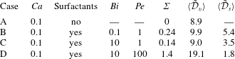
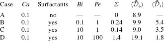
To gain insight into the mechanisms involved during the T1 process, we now characterise the local quantities. We do so for the four illustrative cases A–D given in table 1; they all have
 $Ca=0.1$
but they differ in their Biot and Péclet numbers. The velocity fields, symbolised by arrows, are shown in figure 6. A derived quantity is the local rate of viscous dissipation, defined as (see also appendix B)
 $$\begin{eqnarray}{\mathcal{D}}_{v,loc}=\unicode[STIX]{x1D735}\boldsymbol{u}\boldsymbol{ : }[\unicode[STIX]{x1D707}(\unicode[STIX]{x1D735}\boldsymbol{u}+(\unicode[STIX]{x1D735}\boldsymbol{u})^{\text{T}})],\end{eqnarray}$$
which is shown in figure 7. Finally, the concentration of surfactants is plotted in the bulk (figure 8) and along the interface (figure 9). The snapshots are taken at the following instants: time of the third minimum (
 $t_{1}$
), average value (
 $t_{2}$
), maximum (
 $t_{3}$
) and average value (
 $t_{4}$
) of the capillary force, as defined in figure 4. For convenience of discussion, we identify three distinct types of film (see figure 2): stretched film, which increases in thickness, squeezed film, which decreases in thickness, and the adjacent film separating bubbles laterally.
The velocity field at times
 $t_{1}$
,
 $t_{2}$
,
 $t_{3}$
and
 $t_{4}$
(from left to right) defined in the text and in figure 4 for the cases A, B, C and D (from top to bottom) described in table 1. Arrows represent velocity vectors. The green dotted circle indicates the zone of extensional flow, while the red dashed circles show sheared films.


Our main observations are as follows.
-
(i) In the absence of surfactants, the velocity field is of elongational nature (see the encircled stretched film of case A at instant
$t_{3}$
in figure 6), the velocity vector being almost normal to the interface. The viscous dissipation is significant in the stretched film, but remains low in the squeezed film (see figure 7). -
(ii) The interfacial profile of the surfactants, that is the surface concentration
$f(s)$
along the curvilinear coordinate
$s$
, barely evolves with time during the bubble rearrangement. This is shown in figure 9(a) for case B, but applies more generally. -
(iii) At intermediate Péclet number (
$Pe=1$
), the effect of the Biot number, which characterises the time scale of bulk/interface surfactant exchange (adsorption/desorption), is investigated by comparing case B (
$Bi=0.1$
) and case C (
$Bi=10$
). The influence of the Biot number remains limited when comparing the velocity profile and viscous dissipation distribution, which are quite similar in the two situations. Looking now at the surfactant distribution along the interface, we see from figure 9(b) that it is not homogeneous. This implies that Marangoni stresses are generated at the interface, but they are not sufficient to induce a rigid-like behaviour of the interfaces for the flow (see below). Besides, the inhomogeneities in surfactant distribution are more pronounced at the interface (respectively in the bulk) for small (respectively large)
$Bi$
. This can be understood as follows. At small
$Bi$
, the bulk/interface exchanges are too slow to occur during the course of a rearrangement, while at large
$Bi$
, the gradient in interfacial concentration leads to surfactant desorption (respectively adsorption) in the zone enriched (respectively depleted) in surfactants, which smooths interfacial gradients but induces bulk inhomogeneities. -
(iv) The effect of the Péclet number is investigated by comparing cases C (
$Pe=1$
) and D (
$Pe=100$
). In the latter case, new features appear in the flow. The direction of the velocity seems to be more parallel to the interface; the viscous dissipation is not only located in the stretched film but also in the squeezed one. The shear occurring in the latter (see the squeezed film of case D at times
$t_{1}$
and
$t_{4}$
in figure 6) can only be supported by Marangoni stresses at the interface, where we consistently observe large gradients in interfacial concentration (figure 9
b). These large interfacial gradients also lead to large bulk inhomogeneities in surfactant distribution. It seems that in this case, shearing of the liquid is the main mechanism of foam flow. This last point echoes recent experimental observations in another geometry where switching from an elongational profile to shearing has been observed on varying the surfactant properties (Petit et al.
Reference Petit, Seiwert, Cantat and Biance2015) or deformation rate (Seiwert et al.
Reference Seiwert, Monloubou, Dollet and Cantat2013).


The bulk surfactant concentration
 $F$
at times
 $t_{1}$
,
 $t_{2}$
,
 $t_{3}$
and
 $t_{4}$
(from left to right) defined in the text and in figure 4 for the cases B, C and D (from top to bottom) described in table 1. It should be noted that, for clarity, the
 $F$
scale has been truncated to values below 1.7, while
 $F$
actually takes larger values in case D.

(a) The interfacial surfactant concentration
 $f$
as a function of the curvilinear coordinate
 $s$
(defined in figure 2 and in the inset) for case B (see table 1) at instants
 $t_{1}$
(pink dash-dotted line),
 $t_{2}$
(solid black line),
 $t_{3}$
(red dashed line) and
 $t_{4}$
(blue dotted line) defined in the text and in figure 4. Inset: snapshot of the interfacial surfactant distribution (
 $f$
is colour-coded) at instant
 $t_{3}$
. (b) The interfacial surfactant concentration
 $f$
as a function of
 $s$
at instant
 $t_{3}$
for cases B (red dashed line), C (solid black line) and D (blue dotted line) (see table 1).

4.4 Surface or bulk dissipation
4.4.1 Bulk dissipation
Our qualitative observations indicate that tuning of the surfactant properties (desorption rate, diffusivity) not only affects the elongation of the interfaces and the surfactant distribution, but also the nature of flow, by changing the interfacial boundary condition from a mobile to a rigid-like interface. To put this point on a quantitative basis, we first calculate the total viscous dissipation
 ${\mathcal{D}}_{v}=\int _{V}{\mathcal{D}}_{v,loc}\,\text{d}V$
, with
 ${\mathcal{D}}_{v,loc}$
given by (4.1). The non-dimensional and temporally averaged viscous dissipation rate
 $\langle \tilde{{\mathcal{D}}}_{v}\rangle$
is reported in figure 10 as a function of
 $Pe$
for
 $Ca=0.1$
and
 $Bi=1$
. It exhibits an increase by 60 % in our range of Péclet number at fixed capillary number (i.e. the shear rate). This is only possible if the nature of the flow is fundamentally changing. For shear to exist in the films, the interfacial stress needs to be large enough to sustain the viscous stress at the interface. To verify that this is actually the case, we introduce the ratio
 $$\begin{eqnarray}\unicode[STIX]{x1D6F4}=\frac{h_{min}|\unicode[STIX]{x1D735}_{s}\unicode[STIX]{x1D6FE}|_{max}}{\unicode[STIX]{x1D707}U}.\end{eqnarray}$$
Here,
 $h_{min}$
is the minimum thickness reached during the T1 by the squeezed or stretched films. The ratio
 $\unicode[STIX]{x1D6F4}$
thus compares the maximum value of the Marangoni stress
 $|\unicode[STIX]{x1D735}_{s}\unicode[STIX]{x1D6FE}|_{max}$
along the interface with the typical viscous stress for sheared films
 $\unicode[STIX]{x1D707}U/h_{min}$
. The ratio
 $\unicode[STIX]{x1D6F4}$
is zero for (mobile) stress-free interfaces, while it should be of order 1 for rigid-like interfaces sustaining shear. Values of
 $\unicode[STIX]{x1D6F4}$
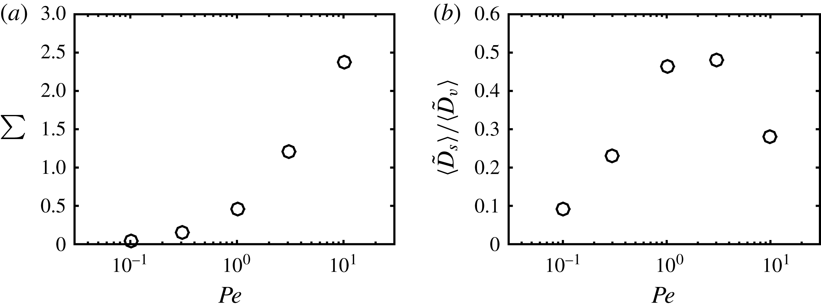
are reported for cases A–D in table 1, and are plotted as a function of the Péclet number in figure 11(a). One can indeed observe that the surface stress becomes comparable to the viscous stress as soon as the Péclet number reaches 2, in full agreement with our previous observations.
The temporally averaged viscous dissipation
 $\langle \tilde{D}_{v}\rangle$
(red circles) and the injected power
 $\langle \tilde{P}_{inj}\rangle$
(black squares) as a function of the Péclet number for
 $Ca=0.1$
and
 $Bi=1$
. The dashed line corresponds to the injected power
 $\langle \tilde{P}_{inj}\rangle$
for the case without surfactants.

(a) The ratio
 $\unicode[STIX]{x1D6F4}$
of Marangoni to viscous shear stress, as defined by (4.2), as a function of
 $Pe$
for the simulations of figure 10. (b) The ratio
 $\langle \tilde{D}_{s}\rangle /\langle \tilde{D}_{v}\rangle$
of the effective surface dissipation over the viscous dissipation, as a function of the Péclet number, for the same simulations.
We now turn to the influence of the capillary number on the viscous dissipation. Figure 12(a) shows that the (time-averaged) dimensionless viscous dissipation
 $\langle \tilde{{\mathcal{D}}_{v}}\rangle$
decreases with the capillary number. This may seem counterintuitive as one expects the dissipation to increase with the velocity, but it should be kept in mind that the actual viscous dissipation corresponds to
 $\langle {\mathcal{D}}_{v}\rangle =\unicode[STIX]{x1D70C}_{l}U^{3}H\langle \tilde{{\mathcal{D}}_{v}}\rangle =\unicode[STIX]{x1D707}_{l}U^{2}\langle \tilde{{\mathcal{D}}_{v}}\rangle$
since we have
 $Re=1$
. This quantity indeed increases with the capillary number but more slowly than
 $Ca^{2}$
, as in the problem of a bubble sliding against a plane (Cantat Reference Cantat2013). This is a consequence of the sublinear behaviour of the total force as a function of
 $Ca$
.
Finally, based on our estimation of the viscous dissipation, we can compare the relative contributions of inertia and viscosity in the flow. As explained in appendix C, and although the Reynolds number is fixed to unity, we have found that the role of inertia remains limited in our simulations, presumably because of the confinement of the liquid films.
(a) The average viscous dissipation
 $\langle \tilde{{\mathcal{D}}}_{v}\rangle$
as a function of
 $Ca$
for different Péclet and Biot numbers (same symbols as in figure 5). (b) The ratio
 $\langle \tilde{{\mathcal{D}}}_{s}\rangle /\langle \tilde{{\mathcal{D}}}_{v}\rangle$
of the effective surface dissipation over the bulk viscous dissipation as a function of
 $Ca$
(same symbols as in figure 5).

4.4.2 Work by surface tension
We have shown that the liquid flow is of a different nature when the surfactant properties are modified, and that at high Péclet number, the distribution of interfacial surfactants becomes increasingly inhomogeneous and the viscous dissipation increases. Now, if we compute the injected power
 ${\mathcal{P}}_{inj}$
(as the plate velocity times the applied force), it is apparent from figure 10 that
 $\langle {\mathcal{P}}_{inj}\rangle$
may be larger than the average viscous dissipation. The difference reveals the work done by surface tension,
 ${\mathcal{D}}_{s}=\int _{\unicode[STIX]{x1D6E4}}\unicode[STIX]{x1D6FE}(\unicode[STIX]{x1D735}_{s}\boldsymbol{\cdot }\boldsymbol{u})\,\text{d}S$
, as discussed in appendix B. This term can be seen as the 2D analogue of the work done by pressure forces in compressible fluids. Numerically, the evaluation of this interfacial quantity is delicate. However, in steady state, the variation of kinetic energy over a rearrangement period should be zero, so that the time-averaged work by surface tension,
 $\langle {\mathcal{D}}_{s}\rangle$
, can be readily calculated as
 $\langle {\mathcal{P}}_{inj}\rangle -\langle {\mathcal{D}}_{v}\rangle$
. Looking at
 $\langle {\mathcal{D}}_{s}\rangle$
as a function of
 $Pe$
, we see from figure 10 that it tends to zero with vanishing
 $Pe$
(in this case, the interface is homogeneous and the surface tension is constant, as in the absence of surfactants), but that otherwise this contribution is positive. This suggests that the work by surface tension may be seen as an effective dissipation on the surfactant-covered interface (hence our notation
 ${\mathcal{D}}_{s}$
). It should be noted that the interfaces considered here have no intrinsic surface viscosities and thus lack the corresponding additional term. However, even without this effect, it is of interest to investigate which contribution, surface or viscous, dominates the dissipation.
Figure 11(b) shows the ratio
 $\langle \tilde{{\mathcal{D}}}_{s}\rangle /\langle \tilde{{\mathcal{D}}}_{v}\rangle$
as a function of the Péclet number for
 $Bi=1$
and
 $Ca=0.1$
. One can observe a maximum (
 ${\approx}0.5$
) reached at intermediate Péclet numbers (
 ${\approx}1$
). This result is reminiscent of the famous model of Lucassen & van den Tempel (Reference Lucassen and van den Tempel1972) for interfacial viscoelasticity: assuming instantaneous adsorption/desorption but diffusion in the bulk, it predicts that the interfacial loss modulus – which characterises the viscous response of the interface – vanishes at both high and small frequencies (analogous to large and small Péclet numbers respectively), but goes through a maximum at intermediate frequencies. Figure 12(b) shows the dependence of
 $\langle \tilde{{\mathcal{D}}}_{s}\rangle /\langle \tilde{{\mathcal{D}}}_{v}\rangle$
as a function of the capillary number
 $Ca$
for different
 $Bi$
and
 $Pe$
parameters. The values of
 $\langle \tilde{{\mathcal{D}}}_{s}\rangle$
and
 $\langle \tilde{{\mathcal{D}}}_{v}\rangle$
for the illustrative cases A–D are also reported in table 1. No clear tendency is visible as the capillary or Biot numbers are changed, but the effect of the Péclet number evidenced above is recovered. (It should be noted that points for the no-surfactant system are also shown in figure 12(b); in this case, the effective surface dissipation should be zero, as the surface tension is uniform. We attribute the comparatively small scatter of the numerical points around the zero value to inaccuracy in the calculation of viscous dissipation due to the non-negligible width of the interfaces in our simulations.)
To recapitulate, the key point is that for all systems considered here, the viscous dissipation is always dominant. This conclusion holds even if the pattern of dissipation is changing with the surfactant properties. At low Péclet number, the interfaces are not able to sustain the viscous stress and the flow is mainly elongational. At intermediate Péclet number, the ratio between surface and bulk dissipation reaches a maximum. This is the threshold above which interfacial stress sustains viscous shear, and viscous dissipation starts to increase with the Péclet number (figure 10). These results are supported by recent experiments in a model system (Petit et al. Reference Petit, Seiwert, Cantat and Biance2015), where the flow in the film was observed to be of elongational or shear type depending on the nature of the surfactants. However, the resulting picture presented here is very different from other scenarios previously put forward in the literature for dissipation. In particular, Tcholakova et al. (Reference Tcholakova, Denkov, Golemanov, Ananthapadmanabhan and Lips2008) showed that surface viscoelasticity can dominate the rheology and the total dissipation in macroscopic foams, while Durand & Stone (Reference Durand and Stone2006) and Biance et al. (Reference Biance, Cohen-Addad and Höhler2009) also concluded that it played the major role in their experiments on T1 dynamics. These point to the role of intrinsic surface viscosities, known to be large in some experimental systems (Golemanov et al. Reference Golemanov, Denkov, Tcholakova, Vethamuthu and Lips2008).
As a final remark, we recall that the liquid fraction in our system is high (
 $\unicode[STIX]{x1D713}_{l}=30\,\%$
), contrary to experiments; we anticipate that the dominant source of dissipation may change at low liquid content. To test this point, we performed additional simulations at
 $Pe=1$
,
 $Bi=1$
and
 $Ca=0.1$
for various liquid fractions in the range
 $\unicode[STIX]{x1D713}_{l}=17\,\%{-}40\,\%$
. These results are shown in figure 13. We found that the injected power
 $\langle \tilde{P}_{inj}\rangle$
decreases with increasing liquid fraction
 $\unicode[STIX]{x1D713}_{l}$
, while the viscous dissipation
 $\langle \tilde{D}_{v}\rangle$
barely changes. This indicates that the effective surface dissipation
 $\langle \tilde{D}_{s}\rangle$
indeed becomes larger for drier foams, as shown in figure 13(b). However, the liquid fraction range remains limited, and additional numerical developments are necessary to reach realistic liquid fractions, as explained in the conclusion.
(a) The temporally averaged viscous dissipation
 $\langle \tilde{D}_{v}\rangle$
(red circles) and injected power
 $\langle \tilde{P}_{inj}\rangle$
(black squares) as a function of the liquid fraction
 $\unicode[STIX]{x1D713}_{l}$
. Other parameters are
 $Ca=0.1$
,
 $Bi=1$
and
 $Pe=1$
. (b) The ratio
 $\langle \tilde{D}_{s}\rangle /\langle \tilde{D}_{v}\rangle$
of the effective surface dissipation over the viscous dissipation as a function of the liquid fraction
 $\unicode[STIX]{x1D713}_{l}$
for the same simulations.

4.5 Film thickness and film rupture
Finally, we examine how the liquid distribution is modified by the coupling between flow and surface tension effects. Observation of the interfaces in the illustrative cases A–D (see figure 6 for instance) indicates that the thickness of the liquid films depends on the parameter set. To analyse this point quantitatively, we extract for each simulation the minimum thickness of the sheared films
 $h_{min}$
(which separate the top bubbles from the bottom ones) as well as
 $h_{min,adj}$
, the minimum thickness between adjacent (top–top or bottom–bottom) bubbles (see figure 2). Figure 14 reports both thicknesses as functions of
 $Ca$
and
 $Pe$
. We observe that
 $h_{min}$
increases with
 $Ca$
, as in the problem of bubbles sliding along a rigid plane (Cantat Reference Cantat2013). Meanwhile, due to volume conservation,
 $h_{min,adj}$
is reduced. Besides, for larger
 $Pe$
,
 $h_{min}$
also increases, as expected for more rigid-like interfaces. These observations have implications for the (in)stability of foams against coalescence. It has been shown (Biance et al.
Reference Biance, Delbos and Pitois2011) that foam collapse, i.e. the occurrence of coalescence avalanches, can be triggered by bubble rearrangements. The suggested mechanism is that some liquid films might become extremely thin in the course of the T1 event, leading to their breaking. Our results may provide information on the probable location of film breaking, which might prove valuable in further studies of foam collapse.
(a) Liquid film thicknesses
 $h_{min}$
and
 $h_{min,adj}$
as a function of
 $Ca$
for
 $Bi=0.1$
and
 $Pe=1$
; (b)
 $h_{min}$
and
 $h_{min,adj}$
as a function of
 $Pe$
for
 $Ca=0.1$
and
 $Bi=1$
. The solid black (respectively dashed red) arrow indicates the value of
 $h_{min}$
(respectively
 $h_{min,adj}$
) without surfactants.

5 Conclusion
We have presented numerical simulations of T1 events in a 2D semiperiodic system of sheared bubbles. The level-set method employed fully accounts for the coupling between the flow dynamics – incompressible Navier–Stokes equations – and the dynamics of surfactants – bulk and interfacial diffusion, as well as bulk/interface exchanges.
Our approach offers a detailed view of all local fields in the course of a bubble rearrangement and enables us to investigate the relative importance of diffusion, desorption/adsorption, viscous effects and surface tension through a parametric study of the Péclet, Biot and capillary numbers. A key result of our simulations is that surfactant inhomogeneities are able to build up Marangoni stresses at the liquid–gas interfaces, with significant consequences on the nature of viscous dissipation, including the appearance of shear flow in the liquid films between the bubbles. We also identify regimes where the work by surface tension leads to an effective surface dissipation, which is reminiscent of the effective surface viscosity developed in the classical model of surface dilatational viscoelasticity by Lucassen & van den Tempel (Reference Lucassen and van den Tempel1972). Besides, we show that as the capillary number increases, the mechanical response of the system is strongly affected by the surfactant dynamics, thus providing microscopic insight to understand foam or emulsion rheology. Finally, our detailed view of liquid distribution in films may provide hints on the possible location for film rupture and subsequent foam collapse.
The perspectives of this work are many, but are all motivated by bringing our simulated systems closer to real foams. So far, the limitations of our system are the following: (i) the geometry is two-dimensional; (ii) the density and viscosity ratios between the liquid and the gas have been set to 10, which implies that the effect of the gas is not negligible as we would expect in real foams; (iii) we only consider the case of bubbles pinned against a solid wall, which hinders the flow and surfactant dynamics compared with bubbles in the bulk of a foam; (iv) we consider a very wet system, with unrealistically thick films. Regarding the first two points, extension to three-dimensional systems and more realistic density and viscosity values is straightforward but will prove demanding in terms of computation time. The third point can be addressed by imposing some pseudoperiodic boundary conditions in the vertical direction – accounting for the opposite velocities between the top and bottom edges. In contrast, new developments will be required to reach the low liquid fractions characteristic of actual foams, including additional terms to prevent bubble coalescence upon contact. In actual foams, coalescence is prevented by non-hydrodynamical forces, such as the disjoining pressure (Israelachvili Reference Israelachvili2010) (including van der Waals, electrostatic or steric interactions), which are short-ranged and thus computationally expensive. These non-hydrodynamic forces are also expected to be crucial in bubble coalescence, and deserve further studies to understand how foam collapse can be triggered by bubble rearrangements. Finally, future work will also account for intrinsic surface dilatational and shear viscosities. This would allow one to assess the relative importance of these contributions in foam rheology, and open the way to a microscopic understanding of the link between foam macroscopic behaviour and interfacial properties.
Acknowledgements
The authors thank the région Rhône-Alpes through ARC Énergies for funding. This work was granted access to the HPC resources of CINES under the allocation A0032B06893 made by GENCI. The authors also thank the méso-centre FLMSN for use of computational resources, and are grateful to Z. Solomenko for his help with the numerical code.
Appendix A. Validation of the numerical method
Several validations have been conducted on the numerical method. First, as regards numerical stability, we first investigated the generation of spurious currents (Solomenko et al.
Reference Solomenko, Spelt, Ó Náraigh and Alix2017), using as a test configuration a bubble at rest. Not only were those currents found to be of negligible magnitude, with a relative velocity variation below
 $10^{-3}$
, but the presence of surfactants actually results in a damping of these unwanted velocity fluctuations. Second, we observed with the initial implementation a significant drift in the total amount of surfactants; the problem was overcome by adjusting the boundary conditions on the plate, as described in § 3.2.1. Finally, a quantitative comparison was made with the results of Teigen et al. (Reference Teigen, Song, Lowengrub and Voigt2011), obtained with a diffuse-interface method. The configuration is close to ours, with a single bubble sheared by the motion of bottom and top plates (figure 15
a). Figure 15(b) shows the surfactant concentration
 $f$
as a function of the position
 $s$
along the interface for several values of the Biot and Péclet numbers. Our curves are in close agreement with those of Teigen et al. (Reference Teigen, Song, Lowengrub and Voigt2011).
Simulations of a sheared droplet. (a) Droplet shape (black) and bulk surfactant concentration (colours) at
 $t=2H/U$
for
 $Bi=20$
,
 $Pe_{F}=8$
and all other parameters set to values similar to those of Teigen et al. (Reference Teigen, Song, Lowengrub and Voigt2011). (b) The interfacial surfactant concentration
 $f$
as a function of the normalised curvilinear coordinate
 $s/s_{max}$
for three parameter sets corresponding to increasing inhomogeneities: (blue)
 $Bi=20$
and
 $Pe_{F}=8$
; (red)
 $Bi=2$
and
 $Pe_{F}=80$
; (black)
 $Bi=0.2$
and
 $Pe_{F}=8$
. The solid lines are results from our level-set simulations, while the dashed lines were obtained by Teigen et al. (Reference Teigen, Song, Lowengrub and Voigt2011) using a diffuse-interface approach. The coordinate
 $s$
increases clockwise, and its origin is shown by the white cross in (a).

Appendix B. Viscous dissipation and work by surface forces
In the following, we detail the different contributions to dissipation in our system. The total variation of kinetic energy
 $K$
is given by
 $$\begin{eqnarray}\frac{\text{d}K}{\text{d}t}=\int _{V}\unicode[STIX]{x1D70C}\boldsymbol{u}\boldsymbol{\cdot }\frac{\text{D}\boldsymbol{u}}{\text{D}t}\,\text{d}V.\end{eqnarray}$$
By substituting the acceleration term from the generalised Navier–Stokes equation (2.4) with the total stress tensor
 $\unicode[STIX]{x1D64F}_{tot}=\unicode[STIX]{x1D748}+\unicode[STIX]{x1D64F}_{s}$
, we obtain
 $$\begin{eqnarray}\frac{\text{d}K}{\text{d}t}=\int _{V}\boldsymbol{u}\boldsymbol{\cdot }(\unicode[STIX]{x1D735}\boldsymbol{\cdot }\unicode[STIX]{x1D64F}_{tot})\text{d}V\end{eqnarray}$$
or
 $$\begin{eqnarray}\frac{\text{d}K}{\text{d}t}=\int _{V}\unicode[STIX]{x1D735}\boldsymbol{\cdot }(\boldsymbol{u}\boldsymbol{\cdot }\unicode[STIX]{x1D64F}_{tot})\,\text{d}V-\int _{V}(\unicode[STIX]{x1D735}\boldsymbol{u}\boldsymbol{ : }\unicode[STIX]{x1D64F}_{tot})\,\text{d}V.\end{eqnarray}$$
Using the Green–Ostrogradsky theorem, the first term can be rewritten as an integral over the volume boundary
 $S$
, here the top and bottom plates,
 $$\begin{eqnarray}\int _{V}\unicode[STIX]{x1D735}\boldsymbol{\cdot }(\boldsymbol{u}\boldsymbol{\cdot }\unicode[STIX]{x1D64F}_{tot})\,\text{d}V=\int _{S}\boldsymbol{u}\boldsymbol{\cdot }\unicode[STIX]{x1D64F}_{tot}\boldsymbol{\cdot }\boldsymbol{n}\,\text{d}S=\int _{S,top}UT_{ext,top}\,\text{d}S-\int _{S,bot}UT_{ext,bot}\,\text{d}S,\end{eqnarray}$$
where
 $T_{ext}$
is the stress exerted on the fluid at the plates and
 $U$
is the plate velocity. Since the total stress includes a bulk contribution (pressure and viscous stress) and a surface one (interfacial stress tensor), this results for the top plate in a viscous contribution, which reads per unit width
 $$\begin{eqnarray}UF_{v}=\int _{S,top}\unicode[STIX]{x1D707}U\frac{\unicode[STIX]{x2202}u_{x}}{\unicode[STIX]{x2202}z}\,\text{d}x,\end{eqnarray}$$
and a capillary one
 $$\begin{eqnarray}UF_{cap}=\mathop{\sum }_{contact\,lines}U\unicode[STIX]{x1D6FE}\cos (\unicode[STIX]{x1D703}),\end{eqnarray}$$
where
 $\unicode[STIX]{x1D703}$
is the angle between the normal to the interface and the
 $z$
-axis. The above two equations are used in §§ 4.1 and 4.2 to compute the forces at the wall. It should be noted also that (B 4) corresponds to the instantaneous injected power
 ${\mathcal{P}}_{inj}$
.
We now focus on the second term on the right-hand side of (B 3), which represents the dissipation rate in the system,
 $$\begin{eqnarray}{\mathcal{D}}=\int _{V}(\unicode[STIX]{x1D735}\boldsymbol{u}\boldsymbol{ : }\unicode[STIX]{x1D64F}_{tot})\,\text{d}V.\end{eqnarray}$$
Use of the expression for the total stress
 $\unicode[STIX]{x1D64F}_{tot}$
and the fact that the flow is incompressible yields
 $$\begin{eqnarray}{\mathcal{D}}={\mathcal{D}}_{v}+{\mathcal{D}}_{s}=\int _{V}\unicode[STIX]{x1D735}\boldsymbol{u}\boldsymbol{ : }[\unicode[STIX]{x1D707}(\unicode[STIX]{x1D735}\boldsymbol{u}+(\unicode[STIX]{x1D735}\boldsymbol{u})^{\text{T}})]\,\text{d}V+\int _{V}\unicode[STIX]{x1D735}\boldsymbol{u}\boldsymbol{ : }\unicode[STIX]{x1D64F}_{s}\,\text{d}V.\end{eqnarray}$$
Whereas the first term
 ${\mathcal{D}}_{v}$
corresponds to the usual viscous dissipation as computed in § 4.4.1, the second term
 ${\mathcal{D}}_{s}$
is a contribution from the liquid–gas interfaces, which can be rewritten as
 $$\begin{eqnarray}{\mathcal{D}}_{s}=\int _{\unicode[STIX]{x1D6E4}}\unicode[STIX]{x1D735}\boldsymbol{u}\boldsymbol{ : }(\unicode[STIX]{x1D6FE}\unicode[STIX]{x1D644}_{s})\,\text{d}S=\int _{\unicode[STIX]{x1D6E4}}\unicode[STIX]{x1D6FE}(\unicode[STIX]{x1D735}_{s}\boldsymbol{\cdot }\boldsymbol{u})\,\text{d}S.\end{eqnarray}$$
The term
 ${\mathcal{D}}_{s}$
can be interpreted as the rate of change of surface energy (Dangla Reference Dangla2012) or as the instantaneous work done by surface tension, a 2D analogue of the work done by pressure forces in compressible fluids. In general, this quantity can take either positive values (e.g. if interfaces are being stretched) or negative values (e.g. for homogeneous
 $\unicode[STIX]{x1D6FE}$
if interfaces are being compressed). It should be noted, however, that if the surface dilatational viscosity
 $\unicode[STIX]{x1D707}_{s}$
were incorporated into the expression of the interfacial stress tensor
 $\unicode[STIX]{x1D64F}_{s}$
(Erni Reference Erni2011; Sagis Reference Sagis2011), this would contribute to
 ${\mathcal{D}}_{s}$
as
 $\int _{\unicode[STIX]{x1D6E4}}\unicode[STIX]{x1D707}_{s}(\unicode[STIX]{x1D735}_{s}\boldsymbol{\cdot }\boldsymbol{u})^{2}\,\text{d}S$
, which is always positive, and indeed corresponds to a true dissipation term.
As the shear-driven T1 events considered in our simulations quickly reach a steady state, we also consider the energy balance (B 3) after time-averaging over one period. Since the kinetic energy is constant on average (
 $\langle \text{d}K/\text{d}t\rangle =0$
), this reduces to
 $$\begin{eqnarray}\langle {\mathcal{P}}_{inj}\rangle =\langle {\mathcal{D}}_{v}\rangle +\langle {\mathcal{D}}_{s}\rangle ,\end{eqnarray}$$
which we use in the present study to estimate the average surface work
 $\langle {\mathcal{D}}_{s}\rangle$
. For interfaces with constant surface tension
 $\unicode[STIX]{x1D6FE}_{0}$
,
 $\langle {\mathcal{D}}_{s}\rangle =\unicode[STIX]{x1D6FE}_{0}\langle \int _{\unicode[STIX]{x1D6E4}}(\unicode[STIX]{x1D735}_{s}\boldsymbol{\cdot }\boldsymbol{u})\,\text{d}S\rangle$
would vanish as the variation in total length averages to zero. However, for surfactant-laden interfaces, we found that
 $\langle {\mathcal{D}}_{s}\rangle$
can be significant in magnitude (
 ${\approx}\langle {\mathcal{D}}_{v}\rangle /2$
), and is generally positive, which we interpret as an effective surface dissipation.
Appendix C. Influence of inertia
Our simulations were conducted for
 $Re=\unicode[STIX]{x1D707}_{l}UH/\unicode[STIX]{x1D70C}_{l}=1$
. The Reynolds number compares inertial and viscous effects, so that inertia is not negligible here a priori. However, in our configuration, viscous flows are mostly confined to the liquid films that separate bubbles, and viscosity may thus dominate inertia. To quantify this point in the illustrative case A (no surfactants,
 $Ca=0.1$
; see table 1), we consider the total kinetic energy of the system
 $K=\int \text{d}V\unicode[STIX]{x1D70C}|\boldsymbol{u}|^{2}$
, which is reported in dimensionless form as a function of time in figure 16. As expected, we find that, after a transient, the kinetic energy oscillates as rearrangements proceed. The average kinetic energy is
 $\langle \tilde{K}\rangle \approx 0.3$
, whereas the oscillation amplitude is of order 0.1 and its period is
 ${\approx}0.6$
, from which we obtain a rough estimate of
 $\text{d}\tilde{K}/\text{d}t\approx 0.2$
. To assess the importance of inertia compared with viscous forces, we finally compare this value with the average viscous dissipation in the same simulation, which is
 $\langle \tilde{{\mathcal{D}}}_{v}\rangle =8.9$
(table 1); as a first approximation, the effect of inertia can be neglected in the present simulations.
The dimensionless kinetic energy
 $\tilde{K}$
as a function of time
 $t$
for case A (see table 1).