


1. Introduction
Our concern is with the instability of the flow in channels of slowly varying depth. In particular, we consider the flow in meandering channels for which the upper wall is located a constant distance in the  $y$ direction from the lower one. We concentrate on centrifugal and elliptical instability mechanisms and show that, in the present context, they are in fact one and the same thing. The choice of the particular meandering geometry enables us to make considerable analytical progress but the approach used applies equally well to the more general case.
Motivation for the type of instability considered here comes from interest in heat transfer mixing devices in laminar flow configurations; see Bergles & Webb (Reference Bergles, Webb, Shenkman, O'Brien, Habib and Kohler1985) and Ligrani, Oliveira & Blaskovich (Reference Ligrani, Oliveira and Blaskovich2003). Our motivation here is to describe the conditions under which laminar centrifugal instabilities can be induced by the channel geometry rather than vortex generators or some device to produce subcritical transition to turbulence. Experimental evidence for the existence of streamwise vortex instabilities in sinusoidal channels is given by Gschwind, Regele & Kottke (Reference Gschwind, Regele and Kottke1995) and Nishimura, Yoshino & Kawamura (Reference Nishimura, Yoshino and Kawamura1987) and Nishimura et al. (Reference Nishimura, Murakami, Arakawa and Kawamura1990a,Reference Nishimura, Yano, Yoshino and Kawamurab). Related instabilities in pipes of periodically varying radius have been found in Navier Stokes simulations by Loh & Blackburn (Reference Loh and Blackburn2011).
Centrifugal instability of a shear layer occurs when Rayleigh's criterion is locally violated. In the flow between concentric cylinders the instability takes the form of Taylor vortices (Taylor Reference Taylor1923) or in the form of Dean vortices if the flow between the cylinders is driven by a pressure gradient (Dean Reference Dean1928). For external boundary layers the instability takes the form of Görtler vortices and, dependent on the shape of the velocity profile, they can occur on either or both concave and convex walls. For the case usually considered, Blasius flow, instability occurs on concave walls.
The property of Görtler vortices distinguishing them from other centrifugal instabilities is that they grow on precisely the same length scale as does the unperturbed flow; see Hall (Reference Hall1982a, Reference Hall1983). Much of the early work on Görtler vortices was influenced by research on Tollmien–Schlichting waves in boundary layers where the fact that the waves occur at relatively high Reynolds numbers makes the use of a quasi-parallel approximation valid; see for example Gaster (Reference Gaster1974). The essential difference between Görtler vortices and Tollmien–Schlichting waves was not appreciated until the work of Hall (Reference Hall1982a, Reference Hall1983). Prior to the latter work there was much confusion as to the nature of the neutral curve with various rather arbitrary effects being used in an attempt to eliminate anomalies found when following a parallel flow approximation; see Görtler (Reference Görtler1941), Smith (Reference Smith1955) and Floryan & Saric (Reference Floryan and Saric1982). However, at high Görtler numbers the local growth rate becomes large and parallel flow theory can be used; see Hall (Reference Hall1982a, Reference Hall1983, Reference Hall1990), Denier, Hall & Seddougui (Reference Denier, Hall and Seddougui1991) and Choudhari, Hall & Street (Reference Choudhari, Hall and Street1994).
The present problem resembles the Görtler instability because we will see that the control parameter associated with the flow varies in the streamwise direction. Elliptical instabilities are usually associated with flows with closed streamlines, see Bayly (Reference Bayly1986), Pierrehumbert (Reference Pierrehumbert1986) and Kerswell (Reference Kerswell2002), and are often viewed as parametric instabilities because of the periodicity constraint enforced on a fluid particle moving on a closed streamline. We shall show that the same instability is operational when periodicity is imposed by channel geometry and, indeed, the instability takes exactly the same form as the right-hand branch Görtler vortex structure uncovered by Hall (Reference Hall1982a). The asymptotic framework we develop shows how to describe the effect of viscosity on elliptical/centrifugal instabilities. Our high wavenumber asymptotic description of streamwise vortices in periodic channels is based on Hall (Reference Hall1982a) but with a non-local effect identical to that found in short wavelength elliptic instabilities present.
In addition to instabilities driven by streamline curvature flows in meandering channels can support Tollmien–Schlichting (TS) waves. This mode of instability occurs in straight channels and there has been much interest in the effect of wall undulations on the waves; see Floryan (Reference Floryan2015). However, transition to turbulence in straight channels occurs through TS waves only if the disturbance environment is extremely quiet. On the other hand the Taylor–Görlter instability leads to a laminar state which can persist into the supercritical regime. For the Taylor problem turbulence follows a wavy vortex instability whilst for the Görtler instability the secondary instability analysis of Hall & Horseman (Reference Hall and Horseman1991) captured the experimentally measured breakdown of Swearingen & Blackwelder (Reference Swearingen and Blackwelder1987); see also Li & Malik (Reference Li and Malik1995). The relative importance of TS waves and centrifugal effects can be gauged by estimating the local Görtler and Reynolds numbers. In fully developed channel flows TS waves occur at Reynolds numbers above 5772 whilst Dean vortices occur when the Dean number is approximately 12. The latter result is important because it shows that even at very small curvatures centrifugal instabilities can dominate the transition process.
The experimental work most relevant to the present work is that of Nishimura et al. (Reference Nishimura, Yano, Yoshino and Kawamura1990b). The latter experiment concerned channels with relatively large wall undulations and it is not clear to what extent the results are influenced by entry effects. Essentially the latter authors found two types of transition to be possible. Firstly an unsteady ‘transverse vortex’ instability of the shear layer adjacent to the troughs and peaks of the channel was observed. Secondly a Taylor–Görtler longitudinal vortex instability was seen in some circumstances; see figure 2 of the latter paper. Here the vortex activity appears to be split into structures associated with and adjacent to the walls. Figure 5 of that paper shows the variation of the critical Reynolds number for each instability as a function of the flow conditions. The nearest theoretical investigation to the latter experimental work is that of Floryan (Reference Floryan2015) who considered much smaller wall undulations. Floryan predicted instability spread across the channel. Essentially the wall undulations apparently destabilise the stable Dean vortex eigenfunctions through a parametric resonance. The reason for the difference in nature of the instability is not clear but we stress that the experiments were for large amplitude oscillations whilst the numerical computations of Floryan were for very small undulations. However, Floryan's results suggest that for small wall amplitudes  $\epsilon$ the critical Reynolds number scales like
 $\epsilon ^m$ where
 $m$ is approximately
 ${-}1.3$; a similar result was found by Floryan (Reference Floryan2002) for Couette flow over a wavy wall.
The above result is at first surprising for the following reasons. Firstly we know from Smith (Reference Smith1979) that at high Reynolds numbers  $R$ and small undulations of amplitude
 $\varGamma$ the definitive scaling is
 $\varGamma \simeq R^{-{({1}/{3})}}$ and the flow splits into a core flow together with boundary layers of depth comparable to the wall undulation amplitude. In the core the streamline curvature there is proportional to
 $\varGamma$ and the local Taylor number is of order
 $R^2 \varGamma$. Based on a local analysis in the streamwise direction it is easy to show that if
 $R$
 $\rightarrow \infty$ with
 $\varGamma$ fixed then instability cannot occur unless the spanwise wavenumber is at least
 $O(\varGamma ^{-({1}/{3})})$ in which case the normal dependence of the vortex must be on the same length scale. Moreover the vortex activity then shifts to the walls and the effective Görtler number for the flow is now
 $R^2 \varGamma ^6$ and so we would anticipate instability when
 $R \simeq {\varGamma ^{-3}}$ is
 $O(1)$. Thus the local theory suggests a quite different scaling than that found in the numerical calculations of Floryan (Reference Floryan2002, Reference Floryan2015) and the centre of vortex activity is in the middle of the channel in the calculations. Note also that the numerical simulations of Cho, Kim & Shin (Reference Cho, Kim and Shin1998) suggest that the dominant velocity component of the streamwise vortex instability is concentrated near the walls for relatively small wall undulations; see figure 11 of the latter paper. However, a local theory points to the vortices being localised near the walls as observed experimentally. The differences between the experiments and local theory compared to the numerical calculations is part of the motivation for the present investigation.
After this paper was submitted an analysis of the small amplitude case for the case when the wall wavelength is comparable to the depth of the channel was given by Hall (Reference Hall2020). There it is shown that in that limit a high Reynolds number vortex–wave interaction theory approach shows that an interaction in a viscous wall layer produces a streamwise vortex instability concentrated over the whole channel. The analysis given in Hall (Reference Hall2020) for the  $O(1)$ wavelength case shows that there the critical Reynolds number varies like
 $\varGamma \simeq {1}/{\varGamma ^{{3}/{2}} \vert \log \varGamma \vert ^{{3}/{4}}}$. Note that the mechanism supporting that mode of instability is absent in slowly varying channels and so there is no overlap with the present case where the small wavenumber–high Reynolds number limit suggests instability when
 $R_m \simeq {1}/{\varGamma ^{3}}$.
In another related paper Hall (Reference Hall2013) investigated the inviscid regime of Görtler vortices on wavy walls. It was shown that wall curvature modulation about a zero mean can induce instability through a parametric resonance. However, that work was limited to high Görtler numbers and curvature modulations on the same length scale that short wavelength Görtler vortices grow. The most relevant previous work on the instability of the flow in meandering channels is due to Floryan (Reference Floryan2015) who considered the same geometry as that discussed here and investigated the instability of the flow to both TS and centrifugal instabilities. Floryan (Reference Floryan2015) considered only the case when the amplitude of the undulations on the wall were typically of size  $10^{-2}$ of the channel depth with wavelength comparable with the channel depth. Here we consider much larger amplitude undulations with a wavelength large compared to the channel depth. Floryan (Reference Floryan2015) restricted attention to modes synchronous with the wall undulations but we shall see below that such a simplification excludes the most dangerous modes in most situations. Nevertheless there is some overlap of our analysis with that of Floryan (Reference Floryan2015) and some limited comparisons of results will be given.
In the next section we will consider the basic flow under consideration using lubrication theory at moderate values of the modified Reynolds numbers and derive the linearised instability equations governing the growth of centrifugal disturbances induced by the wall curvature. In § 3 we will discuss in detail the numerical solution of the disturbance equations for the spatial instability problem and give some limited results for the temporal problem. Section 4 describes the temporal and spatial instability problems in the inviscid limit whilst in § 5 we discuss the right-hand branch problem where the vortices become neutrally stable. In an appendix A we discuss the limiting case of small amplitude wall undulations. Finally in § 6 we draw some conclusions.
2. The base flow and stability equations
We consider the viscous incompressible flow in the sinuous channel defined by
 \begin{equation} h F\left(\frac{x}{L}\right) \le y \le h\left[1+F\left(\frac{x}{L}\right)\right],\quad -\infty < x < \infty. \end{equation}
Here  $h, L$ are typical length scales in the
 $y, x$ directions respectively so that
 $L$ is proportional to the wavelength of the channel. The particular type of channel chosen above is relevant to previous experimental and numerical investigations but is not essential for the theory we will describe. The major simplification is that the base flow in such channels in the limit
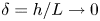 $\delta = {h}/{L} \rightarrow 0$ can be found analytically. More general shapes require a numerical solution, but apart from adding a few modifications to the instability theory described here, the stability discussion remains essentially unchanged. The channel depth is assumed to vary slowly so that
 $\delta ={h}/{L} <\!<1$ and we can use lubrication theory to describe the flow. If the modified Reynolds number defined by
 \begin{equation} R_m= \frac{U_0h^2}{\nu L}, \end{equation}
where  $\nu$ is the kinematic viscosity and
 $U_0$ is a typical
 $x$ velocity is also small the flow will be described by linear lubrication theory. However, we will see that the control parameter for the instability of interest here is in fact
 $R_m$ and so cannot be assumed small. Note that
 $R_m$ being
 $O(1)$ allows for large values of the Reynolds number
 $R_e= {U_0h}/{\nu }$ if
 $\delta$ is taken to be sufficiently small. We introduce dimensionless variables
 $X,Y,Z,T$ by writing
 \begin{equation} (X,Y,Z)=(x/L,y/h,z/h),\quad T=\frac{U_0}{L}t, \end{equation}
and using the usual lubrication theory scalings we write
 \begin{equation} {\boldsymbol{u}}= {{U}_0}\left(\tilde{U}, \frac{h }{L}\tilde{V}, \frac{h }{L}\tilde{W}\right),\quad p=\frac {\mu U_0L}{h^2}\tilde{P}. \end{equation}
The form of the boundaries suggests that we make the Prandtl transformation
 \begin{equation} \zeta= Y-F(X),\quad {\tilde{\boldsymbol{U}}}=(U, V+F' U, W),\quad \tilde{P}=P, \end{equation}
in which case the equations of motion become
 \begin{gather} R_m\frac{\textrm{D} {{U}}}{\textrm{D} T} =-P_X+F'P_{\zeta}+ \nabla^{2}{{U}}, \end{gather}
 \begin{gather}\delta^2 R_m\left[\frac{\textrm{D} {{V}}}{\textrm{D} T}+F''U^2\right] =-P_{\zeta}[(1+ \delta^2{F'}^2)+\delta^2 [F'P_X+ \nabla^{2}{{V}}]+\delta^4[F''' +2 F''{\mathcal{M}}]U, \end{gather}
 \begin{gather}\delta^2 R_m \frac{\textrm{D} {{W}}}{\textrm{D} T} =-P_{Z}+ \delta^2 \nabla^{2}{ {W}}, \end{gather}
 \begin{gather}0= \frac{\partial U}{\partial X}+\frac{\partial V}{\partial \zeta}+\frac{\partial W}{\partial Z}. \end{gather}
Here,  ${\textrm {D} { { }}}/{\textrm {D} T}$ is the convective derivative and
 $\nabla ^2={\partial ^2}/{\partial \zeta ^2}+{\partial ^2}/{\partial Z^2}+\delta ^2{\mathcal {M}}^2$ with
 ${\mathcal {M}}={\partial }/{\partial X}-F'({\partial }/{\partial \zeta })$. The above equations are to be solved subject to
 $\boldsymbol {U}$ vanishing at
 $\zeta = 0, 1$. In the small
 $\delta$ limit with
 $R_m=O(1)$ the basic state takes the form
 \begin{gather} {\boldsymbol{U}} =(\bar{U}(\zeta) ,0,0)+O(\delta^2) =(\zeta-\zeta^2,0,0) +O(\delta^2)+.., \end{gather}
 \begin{gather}P =\bar{P}=-2X -\delta^2\left(F'' R_m\int {\bar{U}}^2\,\textrm{d}\zeta+2F'\zeta\right)+O(\delta^4). \end{gather}
Note that the  $O(\delta ^2)$ term in the pressure is fixed by the
 $\zeta$ momentum equation. The simple base flow given above is valid for all
 $R_m$ in just the same way as plane Poiseuille flow is valid for all Reynolds number. If the walls of the channel are not of the particular assumed form the equations for the mean state have
 $V \ne 0$ and the nonlinear terms do not vanish and the equations must be solved numerically. The corresponding stability problem can be tackled by the approach given below and we will indicate some significant implications for the more general problem later.
2.1. The linear stability equations
The base state under consideration is plane Poiseuille flow parallel to the local wall orientation and is therefore susceptible to 2D Tollmien–Schlichting waves with properties varying locally in  $X$; see, for example, Hall (Reference Hall1982b) and Eagles & Weissman (Reference Eagles and Weissman1975). Here, we concentrate on the potentially much more dangerous modes driven by centrifugal effects associated with streamline curvature. These modes are periodic in the
 $Z$ direction and we therefore perturb the base state to a disturbance of size
 $\epsilon$ by writing
 \begin{gather} U =\bar{U}+\cdots +\epsilon[ {\mathcal{U}}(X,\zeta,Z,T)+ \cdots], \end{gather}
 \begin{gather}V = 0+\cdots +\epsilon[{ \mathcal{V}}(X,\zeta,Z,T)+ \cdots], \end{gather}
 \begin{gather}W = 0+\cdots +\epsilon[{ \mathcal{W}}(X,\zeta,Z,T)+ \cdots ], \end{gather}
 \begin{gather}P = \bar{P}+\cdots +\epsilon\delta^2 [ {\mathcal{P}}(X,\zeta,Z,T)+ \cdots]. \end{gather}
Here, the terms denoted by  $\cdots$ represent terms of smaller size in
 $\delta ^2$ than the preceding terms whilst
 $\epsilon$ is the size of the disturbance and is of course assumed small. Notice above that, following the usual scalings with centrifugal instabilities, the size of the pressure perturbation decreases by
 $O(\delta ^2)$ compared to the velocity components in order to bring both convective and diffusion effects into play in the
 $\zeta , Z$ momentum equations.
Substituting from (2.12)–(2.15) into (2.6)–(2.9) and retaining the leading-order terms in  $\delta ^2$ proportional to
 $\epsilon$ yields
 \begin{gather} \mathcal{L}\mathcal{U } = R_m {\mathcal{V}}\bar{U}', \end{gather}
 \begin{gather}\mathcal{L} \mathcal{V} = {\mathcal{P}_{\zeta}} +2 R_m \bar{U}F'' \mathcal{U}, \end{gather}
 \begin{gather}\mathcal{L} \mathcal{W} = \mathcal{P}_{Z}, \end{gather}
 \begin{gather}0= \frac{\partial \mathcal{U}}{\partial X}+\frac{\partial \mathcal{V}}{\partial \zeta}+\frac{\partial \mathcal{W}}{\partial Z}. \end{gather}
Here, the operator  ${\mathcal {L}}= {\partial ^2}/{\partial \zeta ^2}+{\partial ^2}/{\partial Z^2}-R_m[\bar {U}({\partial }/{\partial X})+ {\partial }/{\partial T}]$. Following Hall (Reference Hall1983) we eliminate
 ${\mathcal {W}},{\mathcal {P}}$ from the above equations to obtain the following coupled equations for
 ${\mathcal {U}}, {\mathcal {V}}$.
 \begin{gather} \mathcal{L}\mathcal{U } =R_m {\mathcal{V}}\bar{U}', \end{gather}
 \begin{gather}{\mathcal{L}} \left[\frac{\partial^2}{\partial \zeta^2}+\frac{\partial^2}{\partial Z^2}\right]\mathcal{V} = 2 R_m \bar{U}F''\frac{\partial^2 { \mathcal{U}}}{\partial Z^2}-R_m \bar{{U}}'' \frac{\partial {\mathcal{V}}}{\partial X}. \end{gather}
Equations (2.20) and (2.21) describe the temporal and spatial evolution of a disturbance present in the flow and we confine our attention to disturbances periodic in the spanwise direction with wavenumber  $k$. The wall curvature leads to the first term on the right hand side of (2.21) and this is the centrifugal term associated with Taylor–Görtler instabilities; rescaling
 $\mathcal {U}$ to be proportional to
 $R_m$ suggests that the effective Görtler number for the flow is
 $R_m^2$. The equations can be related directly to those of Hall (Reference Hall1983) who considered the growing boundary layer problem. In fact the present equations are simpler since the basic state has
 $V=0$. However, the fact that the control parameter
 $R_m$ appears in the operator
 $\mathcal {L}$ has a major effect on the nature of the instability.
The general solution of (2.20) and (2.21) is of course a numerical task and the question arises as to whether spatial or temporal instability is the appropriate description of disturbance growth. We will concentrate on the case when the wall shape is periodic in  $X$. What evidence there is for the absolute/convective nature of the Görtler instability comes from the work of Park & Huerre (Reference Park and Huerre1995) which suggests it is a convective instability. In that case we can drop the time derivative in the equations and treat the problem as a marching problem in
 $X$. However, previous work on the instability problem in meandering channels has used temporal theory so we will give limited results for that case too. Of course neutral stability will occur at the same values of
 $(k, R_m)$ but we will see that there is a significant difference between the behaviour of the temporal and spatial growth rates. In the next section we will first describe the spatial instability problem, the key point about periodic distortions is that spatial instability is now a well-defined notion using Floquet theory. We will then give limited results for the temporal instability case. The numerical work in the next section shows some rather unique but different properties of the temporal and spatial growth rates as the modified Reynolds number increases. The properties suggest some distinct high
 $R_m$ structures which will be described in §§ 4 and 5.
3. Numerical solution of the eigenvalue problem
3.1. Spatial instability approach
We concentrate on periodic channels of the form  $F=\varDelta \cos X$, so that the length
 $L$ introduced earlier is the dimensional wall wavelength divided by
 $2 {\rm \pi}$. Based on the assumption that the instability is convective in nature we find steady solutions of the eigenvalue problem specified by (2.20) and (2.21) with
 $\mathcal {U}, \mathcal {V}, \mathcal {V}'$ vanishing at
 $\zeta =0, 1.$ On the basis of Floquet theory we anticipate a solution with
 ${({\mathcal {U}}, {\mathcal {V}})}= \exp ({[\beta +\textrm {i}\gamma ] X+\textrm {i}kZ})( {{\mathcal {U}} _p(\zeta ,X)}, {{ \mathcal {V }}_p (\zeta , X)})$ where the functions with subscript
 $p$ are periodic functions of
 $X$. Instability is fixed by the sign of
 $\beta$ and solutions with
 $\gamma =0$ are synchronous in
 $X$ with the basic state whilst for example solutions with
 $\gamma =\pm 0.5$ are subharmonic solutions with twice the spatial wavelength of the basic state.
We are primarily interested in finding the most unstable eigenvalue associated with (2.20) and (2.21). If the disturbance is not synchronous with the base flow the two leading-order Floquet exponents will be complex conjugates. If the mode is synchronous then the dominant exponent will correspond to a real Floquet exponent with  $\gamma =0$. Note that if a mode is found then a second one can be generated by the transformation
 $X\rightarrow X+2{\rm \pi}$ and reflecting
 $\zeta$ about
 $\zeta =0.5$. The transformation reflects the fact that if an unstable mode associated with one wall exists then an identical mode associated with the other wall exists. We shall see below that either subharmonic or synchronous can dominate depending on
 $\varDelta$ and
 $R_m$. We shall present preliminary results in this section which will indicate the rather complex eigenvalue structure which develops as
 $R_m$ increases. We will then digress and discuss the high
 $R_m$ limit before returning later to show how that theory explains the numerical calculations at large
 $R_m$.
In order to calculate the complex Floquet exponent  $\beta +\textrm {i}\gamma$ we used two independent approaches. We note that there will be an infinite spectrum of eigenvalues for each
 $(R_m, k)$ but here our primary concern is with the most unstable one. In fact if
 $\beta +\textrm {i}\gamma$ is an eigenvalue then so is
 $\beta -\textrm {i}\gamma$ in which case there is a pair of equally unstable modes. In the first method to solve the eigenvalue problem we modify the approach used for Mathieu's equation and use the fact that if a solution of (2.20) and (2.21) is found by marching in
 $X$ then for large enough
 $X$ it will be dominated by the most unstable mode. If the most unstable mode has
 $\gamma =0$ then some property of that solution evaluated at the beginning and end of a period can be used to obtain
 $\textrm {e}^{2 \beta {\rm \pi}}$ and hence
 $\beta$.
If  $\gamma$ is not zero then that approach fails and we compute two independent solutions of (2.20) and (2.21) by using appropriate initial conditions, here we construct solutions with first
 $u$ and then
 $v$ zero. We then integrate for a sufficiently large range of values of
 $X$ until the solutions are dominated by the two equally unstable Floquet solutions. Typically we found it sufficient to integrate over about 50 periods except where the second most unstable mode had growth rate close to that of the first one. In the latter case it was necessary to integrate over a significantly longer interval but in that situation the second approach outlined below was found to be far more economical. Having integrated for a sufficient interval for the complex conjugate pair of Floquet solutions to dominate some property of each independent solution and the derivative of the property with respect to
 $X$ are calculated at the beginning and end of a period. Since the two solutions are independent then a linear combination of them can be used to represent the dominant Floquet solution. Following the procedure used for Mathieu's equation a little algebra produces a quadratic equation for
 $\exp ({2 [\beta +\textrm {i} \gamma ]{\rm \pi} })$. The latter equation when solved produces the required complex conjugate pair of most unstable modes. Note that if the procedure is used when the most unstable mode is real the procedure produces that mode as a repeated eigenvalue. The equations (2.20) and (2.21) are integrated forward in
 $X$ using the finite difference scheme given in Hall (Reference Hall1983). For the calculations reported on below we found it typically sufficient to use
 $1000$ points in the
 $\zeta$ direction with a step length
 ${2 {\rm \pi}}/{5000}$ in
 $X$.
In the second approach the functions  ${\mathcal {U}}_p(\zeta , X), {\mathcal {V}}_p(\zeta ,X)$ were first expanded as a Fourier series in
 $X$ as
 \begin{equation} {\mathcal{U}}_p(\zeta,X)=\sum_{n=-\infty}^{\infty} {\mathcal{U}}_p^{(n)}(\zeta) \,\textrm{e}^{\textrm{i} n X},\quad {\mathcal{V}}_p(\zeta,X)=\sum_{n=-\infty}^{\infty} {\mathcal{V}}_p^{(n)}(\zeta) \,\textrm{e}^{\textrm{i} n X}. \end{equation}
Substitution of the above into the stability equations gives rise to a coupled system for the Fourier coefficients 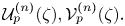 ${\mathcal {U}}_p^{(n)}(\zeta ), {\mathcal {V}}_p^{(n)}(\zeta ).$ Next we truncated the system with
 ${\mathcal {N}}_f$ Fourier modes and used Chebyshev collocation in
 $\zeta$ with
 ${\mathcal {N}}_c+1$ collocation points
 $\zeta _k$ to obtain a generalised eigenvalue problem of the form
 \begin{equation} {\mathcal{A}} {\bf \varPsi}= (\beta + \textrm{i}\gamma){\mathcal{B}} {\bf \varPsi} \end{equation}
for determining the Floquet exponents  $(\beta + \textrm {i}\gamma )$. Here,
 ${\boldsymbol \varPsi }$ represents the vector of unknowns
 ${\mathcal {U}}_p^{(n)}(\zeta _k), {\mathcal {V}}_p^{(n)}(\zeta _k)$ for
 $n=-{\mathcal {N}}_f, \ldots , {\mathcal {N}}_f$ and
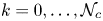 $k=0,\ldots , {\mathcal {N}}_c$. Typically the values
 ${\mathcal {N}}_f=50$ and
 ${\mathcal {N}}_c=60$ were found to be sufficient to give converged results in the most extreme cases. For a given set of parameters, the most unstable eigenvalue was computed using the Arnoldi method using a shift strategy based on simple continuation for the shift values, and in sample cases checks were made by computing the full spectrum.
The two approaches were found to give consistent results. The second approach has the advantage that it produces all the Floquet exponents but it is computationally more expensive. In all cases results were corroborated using both approaches but to save computational time most of the results presented were calculated using the first approach.
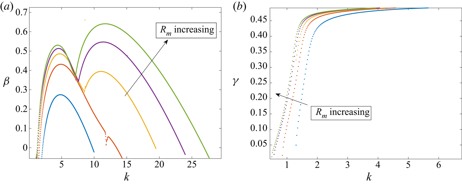
Figure 1 show the real and imaginary parts of the Floquet exponent for  $R_m=1000,2000,3000,4000,5000$ for the case
 $\varDelta =1$. At the points where the growth rate curves have a slope discontinuity the most unstable mode jumps being synchronous to the subharmonic one with
 $\gamma =0.5$ as
 $k$ decreases. All the solutions except the
 $R_m=1000$ case then remain synchronous until they become neutral at the right-hand branch. The
 $R_m=1000$ case does not have the slope discontinuity and is subharmonic when it eventually becomes neutral at the right-hand branch, we will explain that anomalous behaviour in § 5. However, we see that
 $\gamma$ decreases as
 $k$ decreases and so the mode develops as a subharmonic mode with a long wavelength modulation. The point where mode jumping occurs moves to the left with
 $R_m$ increasing. Even at such relatively low values of
 $R_m$ it is apparent that the growth rates to the left of the discontinuity are beginning to asymptote to a limiting form. Note also that moving to the left of the mode-jumping point
 $\gamma$ deceases significantly and so the mode structure is now quasi-periodic in
 $X$. It is also noticeable that the neutral point at small wavenumbers shows little variation with
 $R_m$, we will give an explanation of this when we discuss the inviscid limit.
The spatial growth rate  $\beta$ and
 $\gamma$ the imaginary part of the Floquet exponent as a function of the wavenumber
 $k$ for
 $\varDelta =1$,
 $R_m= 1000,2000,3000,4000,5000$. For the three largest values of
 $R_m$ the quantity
 $\gamma$ changes from zero to 0.5 corresponding to a change from synchronous to a subharmonic one at the slope discontinuities in the panel (a). The quantity
 $\gamma$ then decreases from 0.5 to the left of the discontinuity. For the lowest
 $R_m$ the mode does not become synchronous until higher
 $k$ where it is stable. Note that for
 $R_m=2000$ the slope discontinuity occurs close to the neutral point.

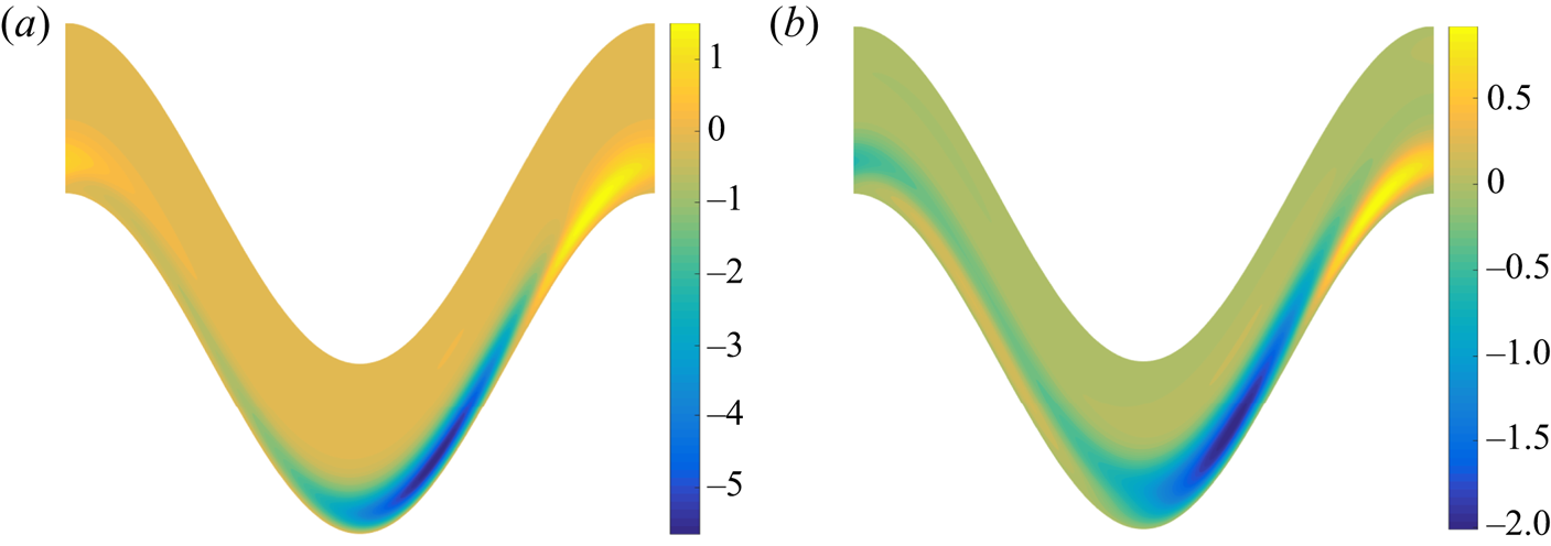
Figure 2 shows the change in form of the  $R_m=5000, \varDelta =1$ streamwise eigenfunction
 ${\mathcal {U}}_p$ when the discontinuity in slope of the
 $R_m=5000$ curve in figure 1 is crossed. Note that the eigenfunction remains synchronous on the whole of that curve to the right of the slope discontinuity. The eigenfunction to the left of the discontinuity is a subharmonic mode and is to be continued in
 $X$ as indicated in the caption. A similar behaviour occurs either side of the discontinuity for the
 $R_m=4000,3000$ cases in figure 1 but with the discontinuity moving to higher wavenumbers so that by the stage that
 $R_m=1000$ all the unstable range of wavenumbers corresponds to the subharmonic mode.
Contours of constant values of the streamwise perturbation velocity 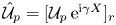 ${\hat {\mathcal {U}}}_p={[{\mathcal {U}}_p \,\textrm {e}^{\textrm {i} \gamma X}]_r}$ at
 $R_m=5000$ with
 $\varDelta =1$ over one wavelength in
 $X$ with
 $0<\zeta <1$. Note the subscript
 $r$ denotes the real part. Panels (a) and (b) correspond to
 $k=7.5, 7.12$, respectively. Panel (a) is synchronous with the basic flow in
 $X$ and so should be continued periodically. The
 $k=7.12$ case is a subharmonic and so is continued in
 $(2 {\rm \pi}, 4 {\rm \pi})$ using
 ${\hat {\mathcal {U}}}_p (\zeta , X)=-{\hat {\mathcal {U}}}_p(\zeta , X-2 {\rm \pi})$ and the pattern then repeats every
 $4 {\rm \pi}$.

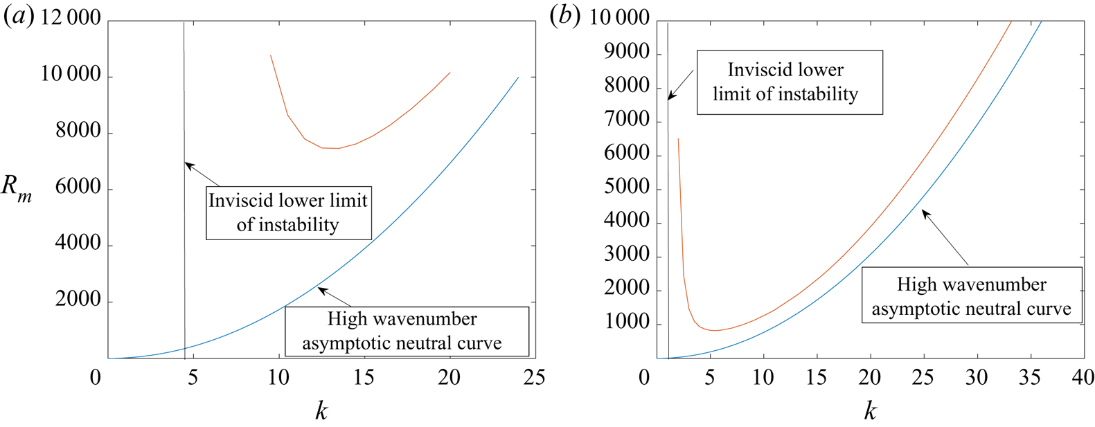
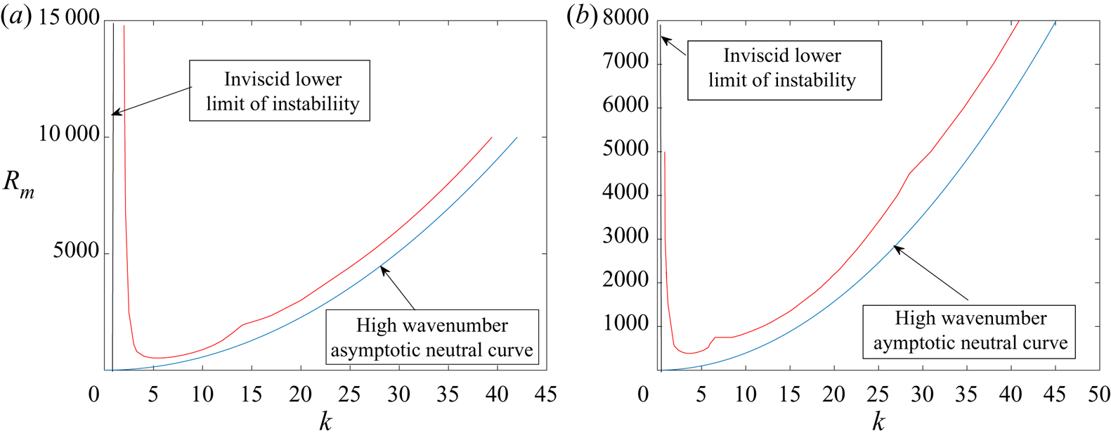
For a given value of  $\varDelta$ we can solve for the Floquet exponent as described above and vary
 $k, R_m$ to produce a neutral curve. Figures 3, 4 show the neutral curves for
 $\varDelta =0.1,0.5, 1,2$. Also shown are the inviscid and large
 $k$ asymptotic predictions of the neutral curves, these will be discussed in §§ 4, 5. We see that on the right-hand branches of the
 $\varDelta =1,2$ curves there are slope discontinuities, these are associated with mode jumping and will be explained in § 5. At the discontinuities the most unstable mode switches from being subharmonic to synchronous, note that there are two discernible such jumps on the
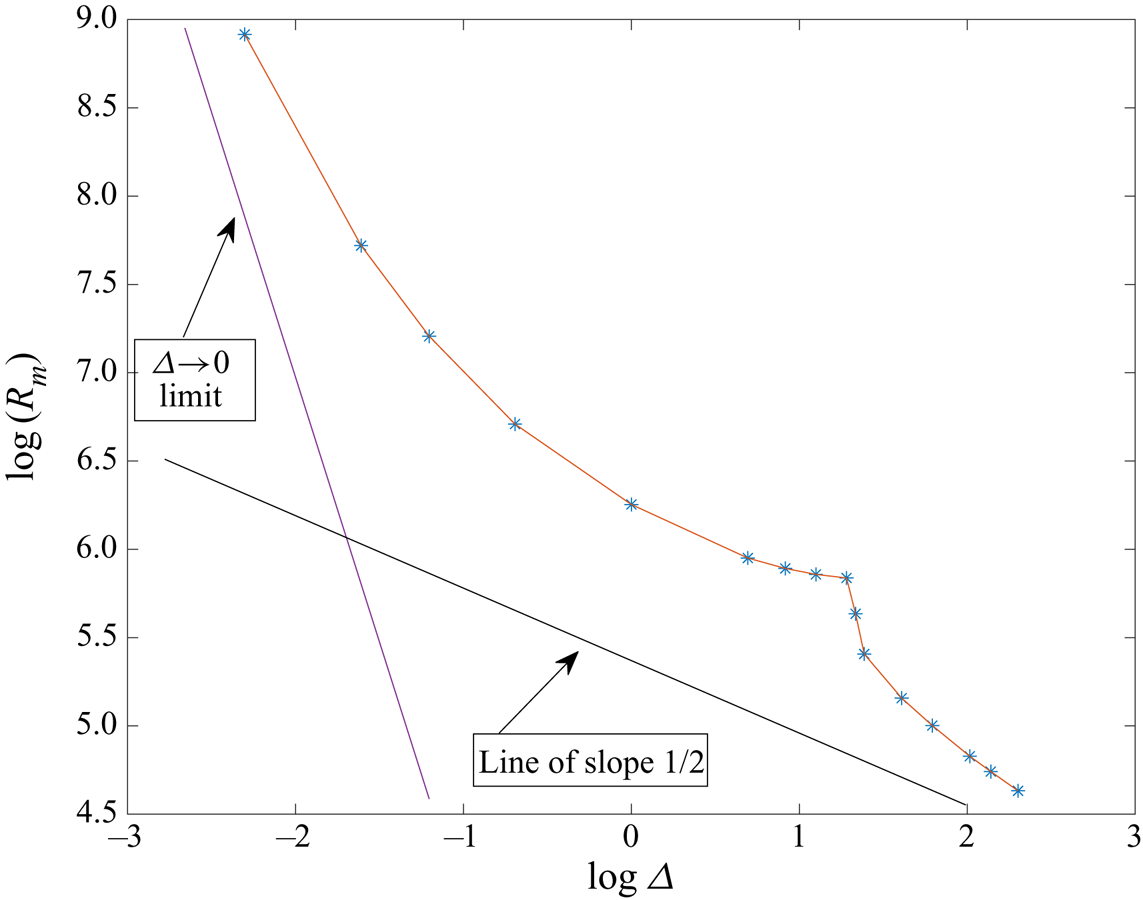
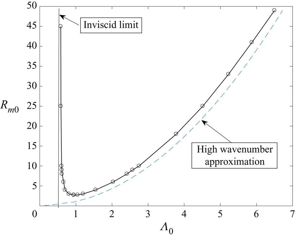
 $\varDelta =2$ curve. The critical value of the modified Reynolds number can be calculated for different values of
 $\varDelta$ and the result of such an exercise is shown in figure 5. Once again the discontinuity of the slope is associated with mode jumping and we observe that the critical value of
 $R_m$ decreases monotonically with
 $\varDelta$. Thus to the left/right of the discontinuity the most dangerous mode is subharmonic/synchronous with the base state.
The neutral curve and its inviscid and large  $k$ forms for
 $\varDelta =0.1, 0.5$ from left to right.

The neutral curve and its inviscid and large  $k$ forms for
 $\varDelta =1,2$ from left to right.

The critical value of the modified Reynolds number  $R_m$ as a function of the wall modulation amplitude
 $\varDelta$. The straight lines shown have slopes
 $-3, -\frac {1}{2}$ and respectively correspond to the small and large
 $\varDelta$ limits.

Later we show the rather remarkable result that the flow is unstable at sufficiently high  $R_m$ for any
 $\varDelta \ne 0$, that is consistent with the assumption that the effective control parameter is
 $R_m^2 \varDelta$. In fact the latter result is only approximately true since, unlike the classical Görtler problem, we cannot combine (2.20) and (2.21) into a single equation involving only
 $R_m^2 \varDelta$.
The question of whether a synchronous or subharmonic mode is the first to become unstable at large  $k$ depends on
 $\varDelta$ and
 $R_m$. Thus, as mentioned already, the observable slope discontinuities on the right-hand branch of the
 $\varDelta =1,2$ curves are associated with mode jumping. Note that as well as the two discernible changes of slope on the
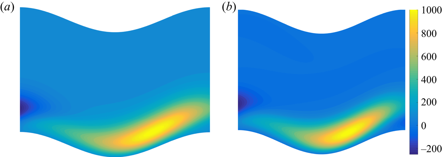
 $\varDelta =2$ neutral curve there are in fact several other mode changes along the right-hand branch. Figure 6 shows the streamwise eigenfunction for
 $R_m=10\,000, \varDelta =0.1$ at
 $k=10,18$. Both modes are subharmonics and are extended to higher values of
 $X$ as indicated in the caption. However, we see that, as in figure 2, the modes are localised near the lower wall. Identical modes associated with the curvature of the upper wall can be found by reflection about the middle of the channel and a translation of half a wavelength in
 $X$.
Contours of constant values of the streamwise perturbation velocity 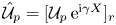 ${\hat {\mathcal {U}}}_p={[{\mathcal {U}}_p \,\textrm {e}^{\textrm {i} \gamma X}]_r}$ at
 $R_m=10\,000$ with
 $\varDelta =0.1$ over one wavelength in
 $X$ with
 $0<\zeta <1$. Panels (a) and (b) correspond to
 $k=10,18$, respectively. Both cases are subharmonic modes to be continued in
 $(2 {\rm \pi}, 4 {\rm \pi})$ using
 ${\hat {\mathcal {U}}}_p(\zeta , X)=-{\hat {\mathcal {U}}}_p(\zeta , X-2 {\rm \pi})$ and the pattern then repeats every
 $4 {\rm \pi}$.

Our calculations at various values of  $\varDelta$ enabled us to draw the following conclusions:
(i) Discontinuities of slope on the neutral curve occur when the most dangerous mode switches from being synchronous to subharmonic in nature.
(ii) The discontinuities occur only on the right-hand branch and, broadly speaking, the number of them increases with
 $\varDelta$.
(iii) For a given
$\varDelta$ and large enough $R_m$ the right hand branch settles down to being either subharmonic or synchronous with no further jumps.(iv) For a given
$\varDelta$ the left-hand branch always corresponds to a subharmonic mode, possibly subject to a long wavelength modulation.


Our results suggest that at large  $R_m$ the right-hand branch moves further to the right- and the left-hand branch occurs at a finite value of
 $k$. In the next section we describe an inviscid asymptotic analysis which captures the large
 $R_m$ structure for
 $O(1)$ values of the wavenumber; following that the subsequent section discusses the right-hand branch. At the end of each section we will compare the relevant asymptotic results with the finite
 $R_m$ computations.
3.2. Temporal instability approach
Here we are interested in solutions of the disturbance equations taking the form
 \begin{equation} {({\mathcal{U}}, {\mathcal{V}})}= \exp({\sigma T +\textrm{i}kZ})({{\mathcal{U}} _p(\zeta,X)}, {{ \mathcal{V }}_p (\zeta, X)}), \end{equation}
where  ${{\mathcal {U}} }_p, {{\mathcal {V}} }_p$ are periodic in
 $X$ with either period
 $2 {\rm \pi}$ or
 $4 {\rm \pi}$ for synchronous or subharmonic modes. Note that previous work seems to have discounted the possibility of a subharmonic response but there is no valid reason to exclude it. Once again, rather than solving the global eigenvalue problem directly, we use solutions obtained by marching the disturbance equations forward in
 $X$ to find the spatial Floquet exponent and then fix
 $\sigma$ by driving the Floquet exponent associated with the marching problem to zero. In other words we simply put an outer Newton iteration loop around the spatial problem described above but with a given value of
 $\sigma$ to produce a solution periodic in
 $0<X<2{\rm \pi}$ or
 $0<X<4{\rm \pi}$. Such a procedure was found to work efficiently everywhere except near the left-hand branch of the neutral curve where modes with comparable growth rate prevent the convergence of the scheme which requires a dominant single or complex conjugate pair of Floquet solutions found by marching. We will first give results for the case
 $\varDelta =1$.
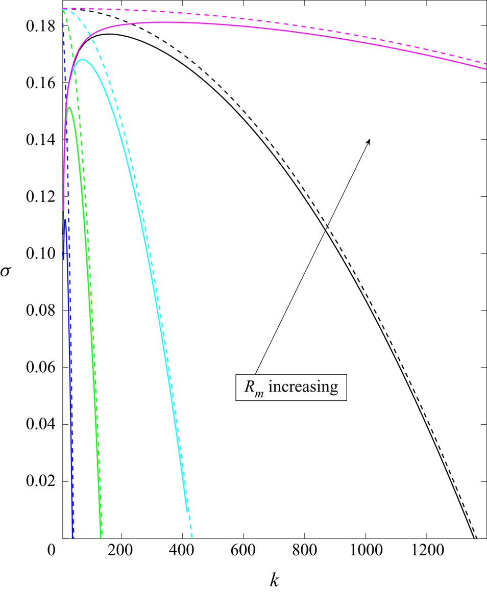
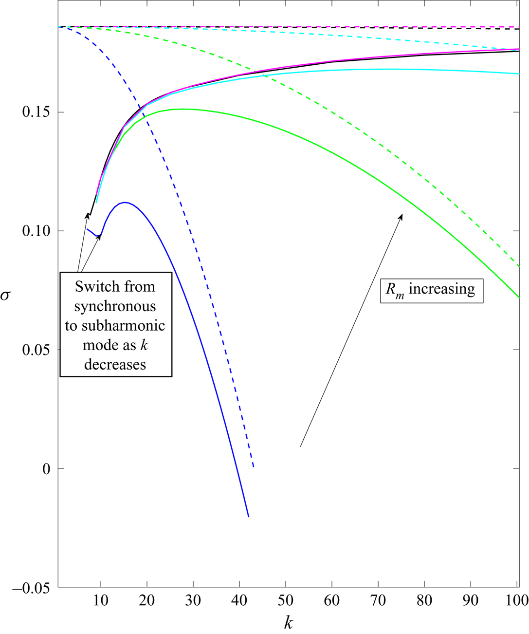
Figures 7 and 8 show plots of the temporal growth rate as a function of  $k$ for
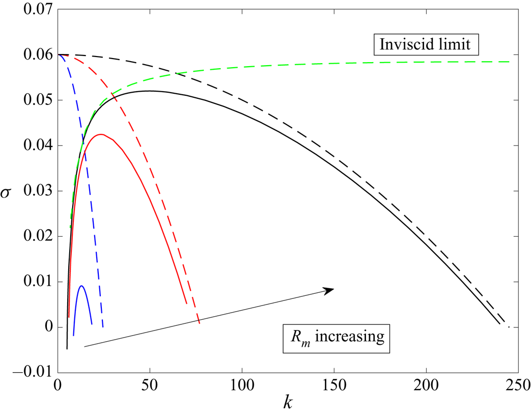
 $R_m=10^4, 10^5, 10^6, 10^7$. Dotted lines represent an asymptotic prediction of the temporal growth rates to be discussed in § 5. Figure 7 shows that as
 $R_m$ increases the curves collapse onto a single curve for a large range of values of
 $k$ but then diverge and pass through zero at appropriate points on the right-hand branch of the neutral curve found earlier using spatial theory. The region where the curves collapse corresponds to the high Reynolds number inviscid temporal instability case which we investigate in the next section. Figure 8 shows the curves in more detail at lower values of
 $k$, note that we were unable to continue the curves to lower values of
 $k$ than those shown because our somewhat inefficient iteration procedure failed when both subharmonic and synchronous modes were possible. Resolution at lower values of
 $k$ requires a direct temporal stability computation beyond the scope of the present investigation and the curves shown all correspond to synchronous modes.
The temporal growth rate  $\sigma$ as a function of
 $k$ for
 $R_m= 10^4, 10^5, 10^6, 10^7, 10^8, \varDelta =1$. The corresponding dashed curves are the asymptotic predictions of
 $\sigma$ near the right-hand branch of the neutral curve.

The temporal growth rate  $\sigma$ at lower values of
 $k$ for
 $R_m= 10^4, 10^5, 10^6, 10^7, 10^8, \varDelta =1$. The corresponding dashed curves are the asymptotic predictions of
 $\sigma$ near the right-hand branch of the neutral curve.

Figure 9 shows results for the temporal growth rate for  $\varDelta =0.1$ and
 $R_m=10^4,10^5,10^6$. All the data points correspond to subharmonic modes and the curve has no slope discontinuities associated with mode jumping. Thus unlike the results for
 $\varDelta =1$ there is no problem with our numerical method as the left-hand branch of the neutral curve is approached. The reason for the different behaviour is explained in §§ 4 and 5. We will see that the left-hand branch necessarily corresponds to a subharmonic mode and the right-hand branch can be either synchronous or subharmonic. When the latter is subharmonic, as in the
 $\varDelta =0.1$ case, the growth rate varies smoothly between the two branches. When the right-hand branch corresponds to a synchronous mode there must be at least one slope discontinuity to account for the required switch from synchronous to subharmonic behaviour as the left-hand branch is approached.
The growth rate  $\sigma$ as a function of
 $k$ for
 $R_m= 10^4, 10^5, 10^6, \varDelta =0.1$. The corresponding dashed curves are the right-hand branch asymptotic predictions of
 $\sigma$. The green curve is the temporal inviscid growth rate discussed in the next section.

We see there is a significant difference from the spatial results shown earlier in figure 1 and further spatial results to be given later in figure 13. The temporal results do not show the regular switch from subharmonic to synchronous modes or the monotonic increase of the spatial growth rate with  $k$; see in particular figure 13. The results of figures 7–9 suggest that the maximum temporal growth rate reaches a finite limiting value as
 $R_m$ increases, whereas the maximum spatial growth rate increases with
 $R_m$, in fact, we find later that it increases like
 $R_m^{{1}/{5}}$.
4. The inviscid limit $R_m \rightarrow \infty , k=O(1)$

It is instructive to understand the limiting forms of the solutions of (2.20) and (2.21) when the modified Reynolds number is large. We discuss the spatial instability case first and return to the temporal case later. For the Görtler vortex problems the different regimes were first identified and described by Denier et al. (Reference Denier, Hall and Seddougui1991); hereafter we refer to the latter as DHS. The key simplifying feature of the large  $G$ limit found in DHS is that, apart from a narrow range of small wavenumbers, the problem becomes quasi-parallel with the three main regions being an inviscid region where the growth rate is
 $O(G^{{1}/{2}})$ for
 $O(1)$ wavenumbers, and two viscous dominated regions where the wavenumbers are
 $O(G^{{1}/{5}}), O(G^{{1}/{4}})$ respectively. The fastest growing mode occurs in the first of those regions and the growth rate reaches
 $O(G^{{3}/{5}})$ there with the vortex structure localised near a boundary. In the
 $O(G^{{1}/{4}})$ wavenumber regime the growth rate falls back to
 $O(G^{{1}/{2}})$ before changing sign at the neutral curve.
The latter regime is the so-called ‘right-hand branch’ structure first identified by Hall (Reference Hall1982a) where the vortices localise in an internal layer so as to maximise their growth. Since the flow is quasi-parallel the latter structures can equivalently be described asymptotically in terms of distance from the leading edge; see Wu, Zhao & Luo (Reference Wu, Zhao and Luo2011). However, note that the claim in the latter paper that a disturbance initiated near the leading edge does not develop into the fastest growing mode downstream is incorrect because the authors overlook the existence of the small wavenumber interactive regime discussed in DHS and Choudhari et al. (Reference Choudhari, Hall and Street1994).
The leading-order approximation to (2.20) and (2.21) in the limit  $R_m \rightarrow \infty$ is
 \begin{gather} \left[\bar{U}\frac{\partial}{\partial X}+ \frac{\partial}{\partial T}\right]{\mathcal{U }} =-{\mathcal{V}}\bar{U}', \end{gather}
 \begin{gather}\left[\bar{U}\frac{\partial}{\partial X}+ \frac{\partial}{\partial T}\right] \left[\frac{\partial^2}{\partial \zeta^2}+\frac{\partial^2}{\partial Z^2}\right] {\mathcal{V}}= -2 \bar{U}F''\frac{\partial^2 { \mathcal{U}}}{\partial Z^2}+ \bar{ {U}}'' \frac{\partial {\mathcal{V}}}{\partial X}, \end{gather}
which must be solved subject to
 \begin{equation} {\mathcal{V}}=0,\quad \zeta=0,1. \end{equation}
Note that in the Görtler problem at large Görtler numbers  $G$ the streamwise length scale shortens to
 $O(G^{-({1}/{2})})$ for large
 $G$ and the stability problem in general becomes quasi-parallel in the
 $X$ direction unless the local wall curvature also varies on the same length scale; see Hall (Reference Hall2013). Note further that the presence of the function
 $F(X)$ in the above system means that we cannot look for spatial or temporal normal modes of the form
 ${\mathcal {V}}=\exp ({{\sigma T} +\textrm {i} k Z}) {\mathcal {V}}_0(\zeta ),$
 ${\mathcal {U}}=\exp ({{\sigma X +\textrm {i} kZ}}){\mathcal {U}} _0(\zeta )$. However, we can make significant analytical progress if we choose to seek steady solutions of the reduced inviscid problem, whether that is the appropriate stability problem must await further work on the absolute convective nature of the instability we consider.
The inviscid Görtler problem is a rather unique non-trivial linear instability problem where there is an exact analytical solution available for any velocity profile; see DHS. Once again we concentrate on the periodic case  $F=\varDelta \cos X$. Following Hall (Reference Hall2013) we can adapt the exact solution of DHS to the non-parallel case by seeking a steady solution separable in
 $X, \zeta$. Thus we write
 \begin{equation} [{\mathcal{U}},{\mathcal{V}} ] = \exp({[{{\pm k \zeta +\textrm{i} kZ}}]})(\varPhi(X) \bar{ {U}}',-\varPhi'(X)\bar{ {U}} ) , \end{equation}
and it is easy to see that (4.1) and (4.2) are satisfied if the function  $\varPhi$ satisfies
 \begin{equation} \varPhi'' \pm F''k \varPhi=0. \end{equation}
The Görtler problem over a wall of constant curvature the corresponding equation has  $F''=1$ and so for wall jets or boundary layers in a semi-infinite region we obtain a spatial growth rate
 $k^{{1}/{2}}$. For the periodic channel problem considered here both signs in the exponential are acceptable with the disturbance concentrated at the upper or lower wall. Note, however, that in the Görtler problem mentioned above the exact solution corresponds to the most unstable mode but other less unstable modes exist. Likewise other modes exist in the present problem but they are not known analytically at finite
 $k$. At large
 $k$ all modes may be found asymptotically but the one considered above is the most unstable one in that regime; in the Görtler problem the exact mode is always the most unstable one. Our finite
 $R_m$ calculations suggest that is also true in the present problem.
Now let us consider the solution of the equation for  $\varPhi$ for periodic channels with
 $F=\varDelta \cos X$. Note that we can without any loss of generality take the spatial period of the wall undulations to be
 $2 {\rm \pi}$, other wavelengths are accommodated by altering the streamwise length scale
 $L.$ However, the wall undulation amplitude
 $\varDelta$ cannot be scaled out of the equations. For the above channel, by letting
 $X \rightarrow x+ {\rm \pi}$, we see that the two
 $\pm$ choices in the exponential term
 ${\textrm {e}^{\pm \zeta }}$ above lead to the same mode with a phase shift of half of wavelength along the channel together with a reflection around the centre of the channel so, without any loss of generality, we take the
 $+$ in the
 $\varPhi$ equation and so we must solve
 \begin{equation} \frac{\textrm{d}^2 \varPhi}{\textrm{d} X^2}- k \varDelta \cos X\varPhi =0. \end{equation}
This is just a particular from of Mathieu's equation which has the standard form
 \begin{equation} \frac{\textrm{d}^2 y}{\textrm{d} x^2}+[a-2q\cos2x]y=0. \end{equation}
Solutions of this equation can be expressed as
 \begin{equation} y=\exp({\nu(a,q)x})\psi_p(x). \end{equation}
Here,  $\psi _p$ is a periodic function of
 $x$ and the Floquet exponent
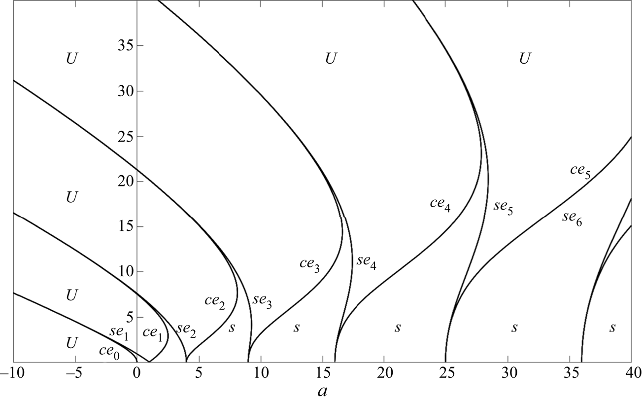
 $\nu =\nu (a,q)$ is either purely imaginary or real corresponding to stable or unstable solutions. Figure 10 summarises the different regions of interest and we see that the
 $\varPhi$ equation corresponds to
 $a=0, q=2{k \varDelta }$. Thus the question of whether solutions of the
 $\varPhi$ equation are stable or unstable is determined by the Floquet exponent
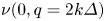 $\nu (0, q=2{k \varDelta })$. Thus from figure 10 we see for a given
 $\varDelta$ the flow is initially stable as
 $k$ increases from zero and then becomes unstable to the subharmonic mode when
 $2{k \varDelta } \simeq 0.92$. This is an important result and says simply that instability cannot occur at high
 $R_m$ unless
 $k> {0.46}/{\varDelta }$. This fixes the left-hand form of the neutral curve for increasing
 $R_m$ and as far as we know, unlike all related Taylor or Görtler instability problems, instability persists only down to a finite wavenumber at high
 $R_m$. The left-hand branch of the neutral curve for a given
 $\varDelta$ therefore always corresponds to a subharmonic mode which is entirely consistent with the finite
 $R_m$ calculations reported on in the previous section.
Stability chart for Mathieu's equation based on Mclachlan (Reference Mclachlan1947). The unstable bands emanate from the points  $a=1,4,9,\ldots$ and the origin. Following the usual notation the even, odd periodic solutions are denoted by
 $ce_0, ce_1, se_1,\ldots$ Stable and unstable regions of parameter space are labelled with
 $S$ and
 $U$ respectively.

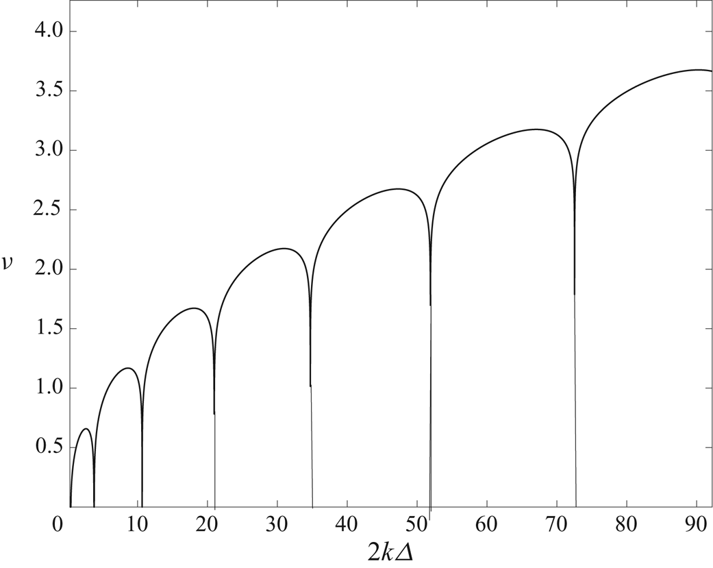
The region of instability beginning at  $2{k \varDelta } \simeq 0.92$ extends to
 $2{k \varDelta } \simeq 8.9$ after which there is a short stable interval followed by another finite band of what is now a synchronous unstable disturbance. That pattern repeats indefinitely and for large
 $k$ the length of the unstable bands and the maximum of the Floquet exponent are both
 $O( 2{k \varDelta })^{{1}/{2}}$. In addition the width of the stable bands tends to zero exponentially for large
 $k$ so the maximum growth rate in each band scales like
 $k^{1/2}$ for large
 $q$. It follows that Floquet solutions of the
 $\varPhi$ equation take the form
 \begin{equation} \varPhi(X)=\exp({{\nu(0, 2 k \varDelta) X}/{2}})\psi_p(X). \end{equation}
Figure 11 is a graph of the real part of the Floquet exponent  $\nu (0, 2 k \varDelta )$ as a function of
 $k \varDelta$; note that the different unstable regimes alternate from being subharmonic to synchronous starting from the left. The above discussion means that in the
 $k$–
 $R_m$ plane the neutral curve has a well-defined left-hand branch given by
 $2{k \varDelta }\simeq 0.92$ and that at small wavenumbers the interactive and non-parallel wavenumber regimes of the Görtler problem described by DHS are absent. We note also from figure 11 that with increasing
 $k$ the fastest growing disturbance in each band becomes increasingly unstable and so the assumption that
 ${\partial }/{\partial X}$ remains
 $O(1)$ in the inviscid limit will fail at large
 $k$. However, the disturbance eigenfunction is proportional to
 $\textrm {e}^{\pm k \zeta }$ and so it becomes concentrated in a thin layer of depth
 $O(k^{-1})$ at the wall. In fact for large
 $k$ we can construct an infinite discrete spectrum of unstable modes following the procedure given in DHS. In that limit we seek a solution in a layer of depth
 $k^{-1}$ and find a set of eigenvalues with growth rate scaling like
 $k^{{1}/{2}}$, the most unstable one of those corresponds to the limiting form of the exact solution discussed above, we do not give details of that calculation here but note that it follows closely the spirit of DHS with solutions expressed in terms of Whittaker functions.
The real part of the Floquet exponent as a function of  $k \varDelta$. Note that apart from the first stable interval on the real axis the other regions are too narrow to be seen on the scale of this plot.

Having now described the inviscid regime we return to interpret the results shown in figure 1 where increasing the modified Reynolds number showed the growth rate curves apparently approaching a limiting form. The liming form is the inviscid structure and figure 12 shows a detailed comparison of the inviscid growth rate with those found by integrating the full equations at increasing values of  $R_m$. We observe that as
 $R_m$ increases the growth rate approaches the inviscid prediction but with the rate of approach decreasing as
 $k$ increases. A comparison of the imaginary part of the Floquet exponents from the inviscid theory and numerical calculations of the full problem shows a similar asymptotic approach of the results.We observe in figure 12 that as
 $k$ increases the finite
 $R_m$ numerical prediction reaches a maximum and then falls off to zero. The interval over which inviscid theory gives an accurate prediction of the spatial growth rate increases with
 $R_m$. We shall comment on the nature of the approach to zero of the growth rates in the following subsection.
Comparison of the growth rates predicted by inviscid theory with full numerical solutions for  $R_m= 10^4, 10^5, 10^6, 10^7$.

Finally in this section we make a few observations on the temporal inviscid instability problem. In that case, assuming a temporal growth rate  $\sigma$ (4.1) and (4.2) and the associated boundary conditions are replaced by
 \begin{gather} \left[\bar{U}\frac{\partial}{\partial X}+ \sigma\right]{\mathcal{U }} =-{\mathcal{V}}\bar{U}', \end{gather}
 \begin{gather}\left[\bar{U}\frac{\partial}{\partial X}+ \sigma\right] \left[\frac{\partial^2}{\partial \zeta^2}-k^2\right] {\mathcal{V}} = 2 k^2 \bar{U}F'' { \mathcal{U} } + \bar{{U}}'' \frac{\partial {\mathcal{V}}}{\partial X}, \end{gather}
 \begin{gather}{\mathcal{V}} =0,\quad \zeta=0,1, \end{gather}
together with  $\mathcal {U}, \mathcal {V}$ being periodic in
 $X$. The solution of the spatial problem at the left-hand limit of wavenumbers satisfies the above system and so temporal neutrality occurs at the same wavenumber as does the spatial case. At finite
 $k$ the above eigenvalue problem must be solved numerically but some observations can be made. Firstly there will be an infinite discrete spectrum of unstable modes which emerge as
 $k$ passes through the values where the unstable spatial modes occur. The temporal inviscid eigenvalue problem can be found from the finite
 $R_m$ temporal algorithm by using increasing values of
 $R_m$ until the growth rate is independent of
 $R_m$. The green curve in figure 9 represents such a calculation for
 $\varDelta =0.1$. We see that as
 $R_m$ increases the growth rate curves approach closer and closer to the inviscid limit. For the highest value of
 $R_m$ shown the green curve and dotted black curve from the right-hand branch asymptotic to be discussed later together give a remarkably good prediction of the growth rate over all
 $k$.
At large  $k$ a solution can be sought with
 $\sigma \simeq O(1)$ and the solution becomes trapped in a layer of thickness
 $O(k^{-{1}/{4}})$. That analysis follows closely the Görtler vortex right-hand branch asymptotics of Hall (Reference Hall1982a) and the recent discussion of inviscid elliptic instabilities given by Banks (Reference Banks2015). The analysis is a limiting version of the right-hand branch viscous problem discussed in the next subsection so we give only the key features here.
We proceed by seeking a structure centred on say the streamline  $\zeta = \bar {\zeta }$ and let
 $\bar {\bar {U}}$ denote
 $\bar { U}$ evaluated at
 $\bar {\zeta }$. Writing
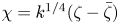 $\chi = k^{{1}/{4}} (\zeta - \bar {\zeta })$ we seek a solution with for example
 ${\mathcal {V}}\sim G(X) S(\chi )$. At leading order we find that
 \begin{equation} \left(\bar{\bar{U}}\frac{\textrm{d}}{\textrm{d} x}+\sigma\right)^2 G=-2\varDelta \cos X \bar{\bar{U}} ' \bar{\bar{U}} G. \end{equation}
Comparing this equation with (4.6) we find
 \begin{equation} \sigma=\frac{1}{2}\bar{U}\nu\left(0,\frac{4 {\rm \Delta} {\bar{\bar{U}}'}}{\bar{\bar{U}}}\right). \end{equation}
For the solution to be trapped in the layer we need  $\sigma$ to be a local maximum when viewed as a function of
 $\bar {\zeta }$. For a given
 $\varDelta$ there will be a sequence of values of
 $\zeta$ where
 $\sigma$ has a local maximum and hence there will be an infinite set of temporal modes. The question of which mode is preferred depends on
 $\varDelta$ and that question will be answered in the next section. Thus as
 $k$ increases the temporal growth rate for each mode will asymptote to a constant. In fact the right-hand branch analysis shows that these match directly onto the limiting small wavenumber form near the right-hand branch so that, unlike the spatial problem, the temporal stability case needs no intermediate wavenumber regime where the inviscid and right-hand branch problems merge. The analysis outlined above is similar that given by Banks (Reference Banks2015) for elliptic instabilities where the vortex structure is trapped around a streamline and we view the above description as a relatively simple way to describe small wavelength elliptic instabilities. Moreover we will now see how the elliptic instability merges naturally onto a similar viscous structure near the right-hand branch.
5. The right-hand branch structure $R_m \rightarrow \infty , k=O(R_m^{{1}/{2}})$

We saw above that at  $O(1)$ wavenumbers inviscid theory accurately describes the spatial growth rate of spanwise periodic vortices. However, when
 $k$ increases for any given large value of
 $R_m$ viscous effects will become increasingly important and stabilise the flow. We also note that on the parts of the curve of growth rate against
 $k$ where the growth rate decreases there are apparently slope discontinuities. That suggests that the discontinuities present in the inviscid spatial instability problem also occur at high wavenumbers where the inviscid theory is no longer relevant.
The effective Görtler number for the flow is of size  $R_m^2$ and so we anticipate that the right-hand branch regime typical of centrifugal instabilities, see Hall (Reference Hall1982a) and DHS, will emerge when the wavenumber is of size
 $R_m^{{1}/{2}}$. For spatially evolving flows the Görtler problem becomes locally a parallel flow problem with the vortex selecting its location normal to the wall in order to maximise its spatial growth rate. In the elliptic instability problem the vortex selects a closed streamline which maximises its temporal growth. In the present problem the spatial instability problem does not become quasi-parallel at large
 $R_m$ and the instability localises on a streamline. For growing boundary layers the temporal instability problem is not well-defined but in the present meandering channel instability problem it is well-defined and again the vortex localises on a streamline. Thus the right-hand branch structure we uncover will be seen to have properties of both centrifugal and elliptic instabilities.
We concentrate once again on the periodic case  $F=\varDelta \cos X$ and seek a solution of (2.20) and (2.21) localised at some height
 $\bar {\zeta }$ for spanwise periodic waves of wavenumber
 \begin{equation} k=\lambda R_m^{{1}/{2}}. \end{equation}
The vortex localises in a layer of depth  $R_m^{-{({1}/{4})}}$ around
 $\bar {\zeta }$ and so we define
 \begin{equation} \eta=R_m^{{1}/{4}}[ \zeta-\bar{\zeta}]. \end{equation}
The dependence of the eigenfunctions in the  $\eta$ direction is in terms of parabolic cylinder functions decaying exponentially torero as
 $\eta \rightarrow \pm \infty$, the first eigenfunction is proportional to
 $\textrm {e}^{-c_0 \eta ^2}$ where
 $c_0$ is a positive constant.
We shall now construct small wavelength solutions of the disturbance equations (2.20) and (2.21) for both the temporal and spatial instability cases. Note that if the approach below is applied to a flow with closed streamlines then only the temporal case is allowable. We expand the base flow as
 \begin{equation} \bar{U}=\bar{U}_0+R_m^{-({1}/{4})} \eta\bar{U}_1+R_m^{-({1}/{2})}\eta^2\bar{U}_2+\cdots. \end{equation}
Note that for the parabolic base flow considered here the higher order terms  $\bar {U}_3, \bar {U}_4$, etc vanish identically. We then write
 \begin{equation} ({\mathcal{U}}, {\mathcal{V}})=\exp({\sigma T+\textrm{i}\lambda R_m^{{1}/{2}}Z}) ({\mathcal{U}}_0, {\mathcal{V}}_0)+R_m^{-{1}/{4}}({\mathcal{U}}_1, {\mathcal{V}}_1)+ R_m^{-({1}/{2})}({\mathcal{U}}_2, {\mathcal{V}}_2)+\cdots,\end{equation}
where  ${\mathcal {U}}_0, {\mathcal {V}}_0$ are functions
 $\eta$ and
 $X$. If we are considering temporal instability for say the periodic channel problem then we require periodicity in
 $X$ for the disturbance and the sign of the real part of
 $\sigma$ will then determine the stability of the flow. For the spatial problem we set
 $\sigma =0$ and seek Floquet solutions in
 $X$ with the real part of the Floquet exponent then determining stability. The above expansions are then substituted into (2.20) and (2.21) and like powers of
 $R^{-({1}/{4})}$ are equated. The leading order approximations to the latter equations yields a pair of coupled equations for
 ${\mathcal {U}}_0, {\mathcal {V}}_0$ which can be combined to give
 \begin{equation} \left(\lambda^2+\sigma+\bar{U}_0\frac{\textrm{d}}{\textrm{d} X}\right)^2{\mathcal{U}}_0=-2 {\rm \Delta} \bar{U}_0\bar{U}_1 \cos X {\mathcal{U}}_0. \end{equation}
For the Görtler problem the corresponding equation is an algebraic equation for the spatial growth rate whereas here the spatial instability growth rate comes from the Floquet exponent associated with (5.5). If we consider the temporal instability case then
 \begin{equation} \sigma=\sigma(\bar{\zeta} )=-\lambda^2+\frac{1}{2}\bar{U}_0\nu \left(0, \frac{4 \bar{U}_1 \varDelta }{{\bar{U}_0}}\right),\quad {\mathcal{U}}_0=Q(X), \end{equation}
where  $\nu (a,q)$ is the Floquet exponent of Mathieu's equation and
 $Q$ is the associated periodic function of
 $X$. For spatial instability
 \begin{equation} {\mathcal{U}}_0=\textrm{e}^{ \beta X }Q(X), \end{equation}
and the spatial growth rate  $\beta$ is given by
 \begin{equation} \beta= \beta(\bar{\zeta} )= -\frac{\lambda^2 }{\bar{U}_0}+\frac{1}{2}\nu \left(0, \frac{4 \bar{U}_1 \varDelta }{{\bar{U}_0} }\right). \end{equation}
Neutral stability in both cases yields
 \begin{equation} \lambda^2=\frac{1}{2}\bar{U}_0\nu\left(0, \frac{4 \bar{U}_1 \varDelta }{{\bar{U}_0} }\right), \end{equation}
and in either case at next order in  $R_m^{-({1}/{4})}$ we obtain
 \begin{equation} \left(\lambda^2+\sigma+\bar{U}_0\frac{\textrm{d}}{\textrm{d} X}\right)^2{\mathcal{U}}_1+2 {\rm \Delta} \bar{U}_0\bar{U}_1 \cos X {\mathcal{U}}_1=\eta F_1(X). \end{equation}
Here,  $F_1$ is determined in terms of the leading-order solution and a solvability condition given by the vanishing of the integral over a period of
 $F_1$ multiplied by the adjoint of
 $Q$ is required for a solution to exist. It is straightforward to show that for the temporal case the required condition is
 \begin{equation} \frac{\textrm{d} \sigma}{\textrm{d} \bar{\zeta}}=0, \end{equation}
whilst for the spatial case we need
 \begin{equation} \frac{\textrm{d} \beta}{\textrm{d} \bar{\zeta}}=0, \end{equation}
and it can be shown that these conditions are the same for neutral modes. Once again it is instructive to point out how the analysis here deviates from that for the Görtler problem. Thus in that problem (5.10) would be an algebraic equation at each  $X$ and we would need to choose
 $F_1=0$ at each
 $X$ which maximises the local spatial growth rate. In the present problem the growth rate depends on a global condition associated with periodicity in
 $X$.
At order  $R_m^{-({1}/{2})}$ we obtain
 \begin{align} \left(\lambda^2+\sigma+\bar{U}_0\frac{\textrm{d}}{\textrm{d} X}\right)^2{\mathcal{U}}_2+2 {\rm \Delta} \bar{U}_0\bar{U}_1 \cos X {\mathcal{U}}_2=\eta^2 F_2(X){\mathcal{U}}_0+F_3(X) \frac{\textrm{d}^2 {\mathcal{U}}_0}{\textrm{d}\eta ^2}+F_4(X){\mathcal{U}}_0. \end{align}
Here,  $F_4(X)$ will include terms proportional to the higher-order terms in the temporal or spatial growth rate together with a correction term to
 $k$. Application of the required solvability equation will produce an equation of the form
 \begin{equation} \frac{\textrm{d}^2 {\mathcal{U}}_0}{\textrm{d}\eta ^2} -a_1{\eta^2 \mathcal{U}}_0-a_2{{\mathcal{U }}}_0=0. \end{equation}
The fact that the growth rate was maximised over  $\bar{\zeta}$ means that
 $a_1>0$ and then the requirement that the solutions decays to zero at
 $\pm \infty$ fixes
 $a_2$ which in turn determines the next order growth rate. If we seek neutral solutions then the latter choice of
 $a_2$ gives the higher-order correction to
 $k=\lambda R_m^{{1}/{2}}$.
5.1. Results for the spatial case
It is sufficient to consider only  $\frac {1}{2}<\zeta <1$ since results for the lower half of the channel are then found by reflecting about the channel centre and changing
 $X\rightarrow X+ {\rm \pi}$. Solutions to the spatial problem are found by
(i) Setting
$\sigma =0$ and for given $\lambda , \varDelta$ computing $\beta$ at each $\zeta$ in $(\frac {1}{2},1)$.(ii) Checking whether the current value of
$\zeta$ corresponds to a local maximum of $\beta$.


It is easy to see from figure 11 that there will be an infinite number of values  $\bar {\zeta }$ where
 $\beta$ has a local maximum and that when
 $\lambda \rightarrow 0$ the maxima will correspond directly with the maxima of figure 11. A given mode will be neutral when
 $\lambda ^2=\frac {1}{2}\bar {U}_0\nu (0, {4 \bar {U}_1 \varDelta }/{{\bar {U}_0}})$ and when
 $\lambda$ is decreased from its neutral value
 ${\bar {\zeta }}$ will increase to a constant value at
 $\lambda =0$. Moreover as the mode number increases the latter constant values will approach
 $\bar {\zeta }=1$ with the corresponding growth rates tending to infinity in that limit.
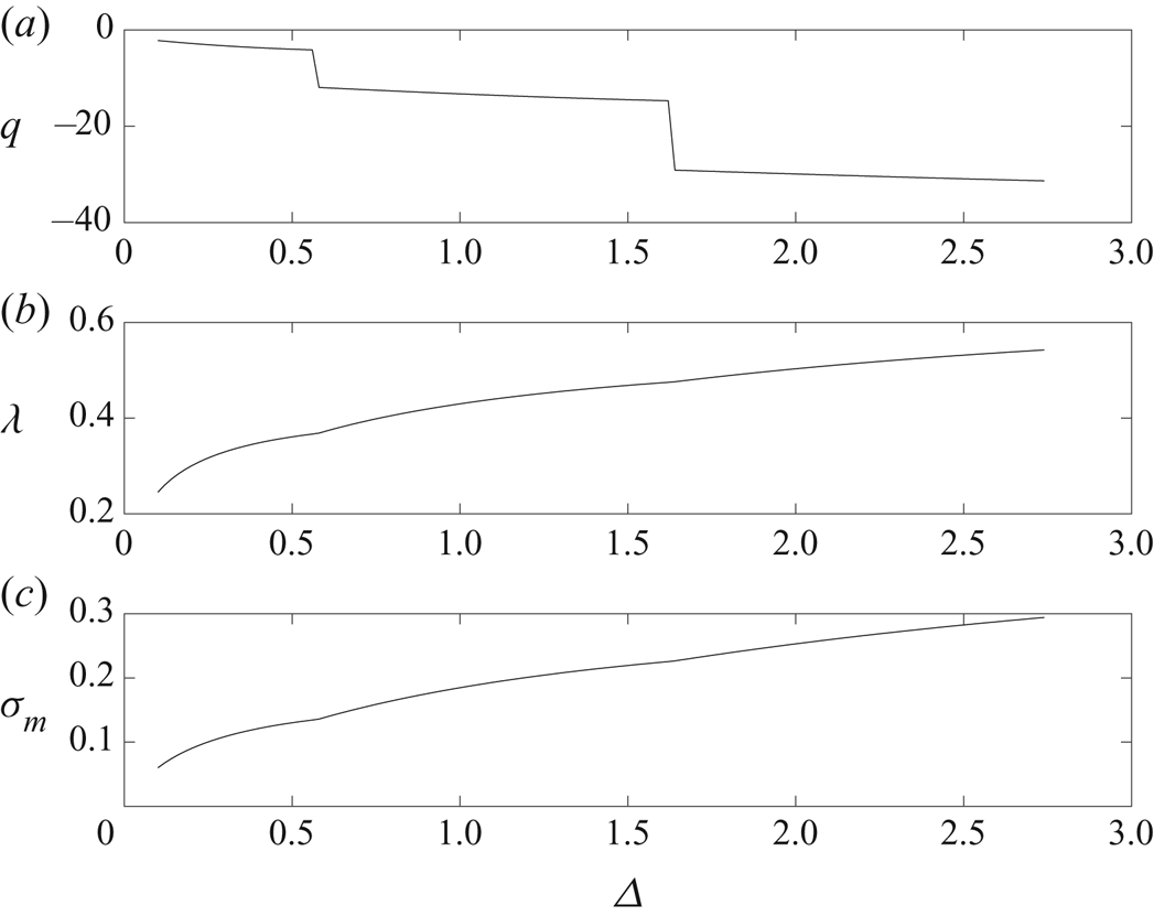
The situation is similar to the inviscid problem where there are two identical families of modes centred on points in the lower/upper parts of the channel. We will give results for modes concentrated in the upper half and in the middle panel of figure 13 we show how the neutral value of  $\lambda$ varies with
 $\varDelta$. The value of the associated
 $q$ in Mathieu's equation is plotted in the upper part of that figure. We see that as
 $\varDelta$ increases from zero the first mode to become unstable is the subharmonic and has
 $q$ on the first hump of figure 11. However, at
 $\varDelta \simeq 0.57$ the synchronous mode corresponding to the second hump becomes the first to become unstable. A further increase in
 $\varDelta$ shows that the first unstable mode jumps to a subharmonic one associated with the third hump of figure 11 when
 $\varDelta$ is approximately 1.63. That process continues indefinitely as
 $\varDelta$ increases with the first mode to become unstable moving from left to right across the humps of figure 11. The associated value of
 $\bar {\zeta }$ has similar jumps as
 $\varDelta$ is increased with the values approaching 1 monotonically.
Panels (a) and (b) show dependence of the constant  $q$ in Mathieu's equation and the value of
 $\lambda$ where the first neutral mode occurs as a function of
 $\varDelta$ in the spatial problem. The jumps in
 $q$ correspond to the local maximum of the spatial growth rate switching between the different ‘humps’ in figure 11. Panel (c) shows
 $\sigma _m$ the maximum growth rate of the temporal problem over all
 $\lambda$ as a function of
 $\varDelta$.

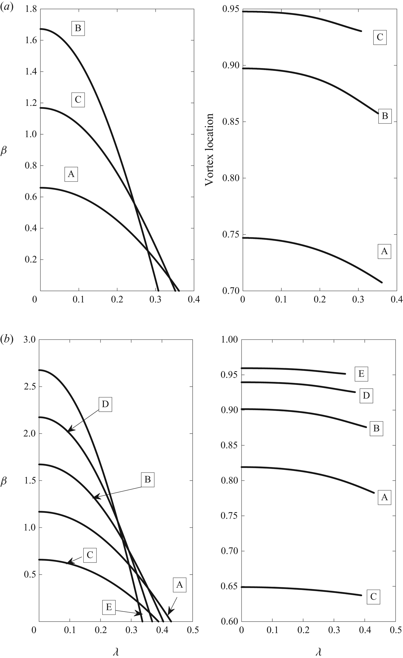
The left-hand panels of figure 14 show the spatial growth rate as a function of  $\lambda$ for the first few modes of the
 $\varDelta =0.5,1$ cases. The right-hand panel shows
 $\bar {\zeta }$ the corresponding location of the transition layer. We see that
 $\bar {\zeta }$ for each mode increases monotonically to a constant at
 $\lambda =0$. The fact that the value of
 $\bar {\zeta }$ for the first mode to become unstable is the second curve up from the bottom of the lower figure reflects that the fact that this mode is associated with the second hump of figure 11 and so requires a higher value of
 $\bar {\zeta }$ in order to achieve the required value of
 $q$.
(a) The spatial growth rate  $\beta$ for
 $\varDelta =0.5$ as a function of
 $\lambda$ and the location of the modes as
 $\lambda$ varies. (b) The spatial growth rate
 $\beta$ for
 $\varDelta =1$ as a function of
 $\lambda$ and the location of the modes as
 $\lambda$ varies. The labels A, B, show which growth rate curve relates to the mode location.

Results for higher values of  $\varDelta$ are broadly similar to those for the above cases with the curve
 $\bar {\zeta }=\bar {\zeta }(\lambda )$ moving upwards as
 $\varDelta$ increases so as to facilitate the associated value of
 $q$ to be sufficiently high for the solution to be associated with progressively higher humps in figure 11. The upshot of that is that as
 $\varDelta$ increases the curves become closely packed with the modes rapidly swapping order of importance in terms of growth rate as
 $\lambda$ decreases.
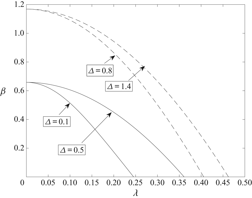
Figure 15 shows the spatial growth rate as a function of  $\lambda$ for 4 values of
 $\varDelta$. The lower two values of
 $\varDelta$ are associated with the first hump of figure 8 and the other two with the second hump. The curves show that as
 $\lambda$ approaches zero the growth rate for values of
 $\varDelta$ associated with the same hump tend to the same constant and that those constants are different for different humps. That result follows from the maximisation of
 $\beta$ for
 $\lambda =0$ which requires that the associated value of
 $q$ must correspond exactly to the relevant maximum location in figure 11. That is achieved for a given
 $\varDelta$ by selecting the appropriate
 $\bar {\zeta }$ to make
 ${4 \bar {U}_1 \varDelta }/{{\bar {U}_0}}$ equal to the value of
 $q$ at the relevant maximum of figure 11. The values of
 $\bar {\zeta }$ selected will vary with
 $\varDelta$ but all will correspond to the same numerical value of
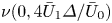 $\nu (0, {4 \bar {U}_1 \varDelta }/{ {\bar {U}_0}})$ which gives the growth rate.
The spatial growth rates  $\beta$, for
 $\varDelta =0.1,0.5,0.8,1.4$ as a function of
 $\lambda$ for the first eigenvalue to become unstable. Note the curves for the smallest two values of
 $\varDelta$ asymptote to the same value since they both correspond to solutions at the maximum of the first hump of figure 11. Likewise the two larger values asymptote to the maximum of the second hump of figure 11.

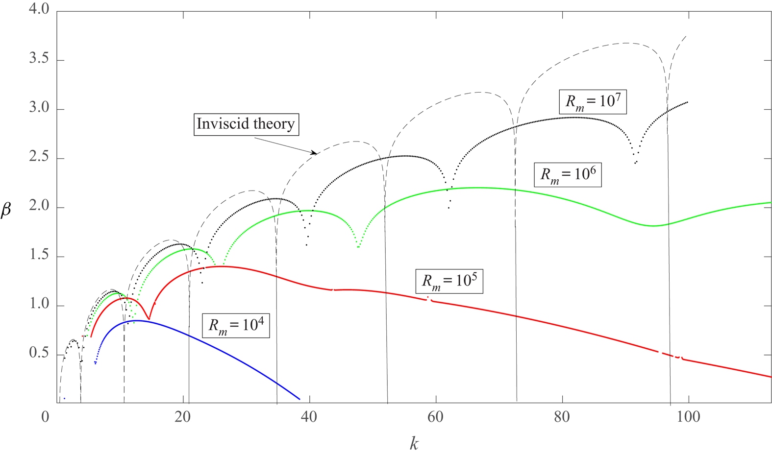
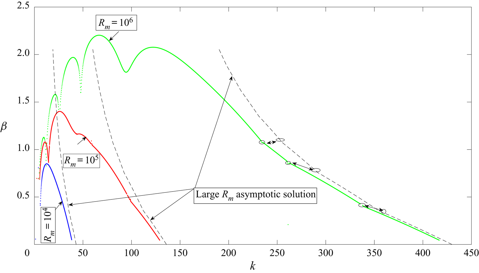
In figure 16 we compare the right-hand branch growth rate predictions with the finite  $R_m$ calculations at increasing values of
 $R_m$. The dashed curves correspond to the predictions from the right-hand branch theory. To plot the curves we need to compute the value of
 $\lambda$ using
 $k=\lambda R_m^{{1}/{2}}$ and then find the most unstable right-hand branch mode at the current value of
 $\lambda$. The ellipses on the dashed curve for
 $R_m= 10^6$ correspond to points where the most unstable mode jumps. The arrows show the correspondence of those points with changes of slope on the
 $R_m=10^6$ finite
 $R_m$ curve. We see that the right-hand branch structure accurately predicts the growth rates and discontinuities over quite a large range of
 $k$.
Growth rates as a function of  $k$ for
 $\varDelta =1$ at fixed values of
 $R_m=10^4, 10^5, 10^6$. Also shown are the corresponding large wavenumber asymptotic approximations to the growth rates. Note the discontinuities in slope marked by the ellipses for the
 $R_m=10^6$ case. The arrows show the relationship between the numerical and asymptotic predictions of slope discontinuities.

5.2. Results for the temporal case
Results for the temporal case are found using a similar procedure but with now  $\bar {\zeta }$ fixed by maximising
 $\sigma$ rather than the spatial growth rate. The neutral modes of the spatial problem correspond identically to the neutral modes of the temporal problem and so figure 14 applies to both the spatial and temporal problems and the first mode to become unstable as
 $\lambda$ decreases will be a function of
 $\varDelta$ and will jump between the humps of figure 11 as
 $\varDelta$ increases. However, for the temporal problem the quantity
 $\bar {\zeta }$ is independent of
 $\lambda$ so that the growth rate curves emanating from the different neutral points at decreasing values of
 $\varDelta$ cannot cross and the first mode to become unstable will always have the largest temporal growth rate. Moreover the quantity
 $\sigma _m$ which is the maximum value of the growth rate over
 $\lambda$ will occur when
 $\lambda =0$ and is equal to
 $\bar {U}\nu (0, {4 \bar {U}_1 \varDelta }/{{\bar {U}_0} })$ evaluated at the value of
 $\bar {\zeta }$ at the neutral point. It follows then that the maximum growth rate is simply
 $\lambda ^2$ at the neutral point. But note again that the most unstable mode will be subharmonic or synchronous depending on which hump of figure 11 the solution is associated with, our results suggest that the relevant hump increases with
 $\varDelta$. Now let us turn to the temporal growth rate prediction associated with the right-hand branch. In fact the temporal predictions were already shown in figures 7–9. We see the remarkably accurate predictions made by the large
 $k$ asymptotic solutions and, as remarked earlier, taken together the inviscid and right-hand branch asymptotic predictions of the temporal growth rate provide an accurate approximation to the growth rate over all
 $k$.
We conclude from the above discussion that there is a clear link between the small wavelength form of the elliptic instabilities of Bayly (Reference Bayly1986) and Pierrehumbert (Reference Pierrehumbert1986). In the latter papers the authors were concerned with flows with closed streamlines but their arguments apply equally to spatially periodic flows. Thus the elliptic instability at large  $k$ of the inviscid problem merges directly onto the small wavenumber viscous right-hand branch structure of Hall (Reference Hall1982a). That raises the possibility of extending the elliptic instability problems in flows with closed streamlines into the viscous regime.
5.3. The fastest growing mode for spatial instability
We have seen above that
(i) The inviscid spatial mode localises near the wall and has growth rate increasing like
$k^{{1}/{2}}$ for large $k$.(ii) The right-hand branch modes cluster near the wall as
$\lambda \rightarrow 0$


The inviscid structure then breaks down when the initially passive viscous layer associated with an inviscid mode is the same size as the wall layer of thickness  $k^{-1}$ where the fastest growing inviscid mode localises for large
 $k$. Likewise the right-hand branch structure fails when the layer around
 $\bar {\zeta }$ is the same size as its distance from the wall. That breakdown is essentially the same as that discussed in DHS for what the latter authors referred to as the fastest growing mode. The discussion here is closely related to DHS and so we will give only brief details. The scalings used follow from the above discussion and differences from those in DHS arise because in the present problem the
 $X$ derivatives are multiplied by
 $R_m.$ Since the spatial growth rate becomes large in both limiting cases the stability problem becomes quasi-parallel in this limit. It can be shown that the wavenumber overlap region where the inviscid and right-hand branch modes meet has
 $k= O(R_m^{{2}/{5}})$ and the modes occupy layers of thickness
 $O( R_m^{-({2}/{5})})$ at the walls and viscosity can no longer be neglected. The structure is similar to that given in DHS but more complex because there is now a WKB structure in
 $X$ with transition layers where the curvature changes sign. We do not pursue it here because our numerical results suggest the modified Reynolds number needs to be bigger than
 $10^6$ before it is relevant, and at such high
 $R_m$ it is therefore perhaps not physically relevant.
6. Conclusion
We have investigated the spatial and temporal instability of the flow in a meandering channel. We have concentrated on the spatial case because the only investigation of the absolute/convective nature of the Görtler instability showed that it was in fact a convective instability. However, the geometry considered here is somewhat different with a flow periodic in the streamwise direction.
If the channel is not of the particular type of meandering one considered here the basic flow must be found numerically at finite  $R_m$. In that case reversed flow occurs in the ‘valleys’ and we would certainly anticipate that the instability associated with such reversed flow regions would be an absolute instability. However, the approach we have used here is applicable to more general channel shapes but the disturbance equations become rather messier but they retain the basic properties of (2.20) and (2.21).
The most closely related work is that of Floryan (Reference Floryan2015) who considered meandering channels with small amplitude undulations of wavelength comparable to the channel depth, in other words channels with  $\delta =1$. Floryan ignored the possibility of subharmonic modes so gave results only for those synchronous with the basic state in
 $X$. Floryan found eigenfunctions distributed across the channel with no apparent concentration near either wall. However, Floryan reports that the modes he found cut out at an
 $O(1)$ value of the channel wavelength and so presumably they do not exist in the present configuration. The disturbances computed here, and indeed the asymptotic approximations to them, all show a tendency to localise near either wall.
The reason for the apparent difference in form of the disturbances found here with those of Floryan is therefore likely to be that at large channel wavelengths the preferred mode localises near the walls. The numerical scheme we used to march the equations in  $X$ correctly predicts growth rates found elsewhere for Görtler instabilities and our calculated growth rates are consistent with the asymptotic analysis. Thus it would appear that, in Floryan's case, channels of wavelength comparable with the channel depth support instabilities distributed across the channel because of the rapid change of sign of the curvature in the downstream direction. Floryan's results are all for wall amplitudes of size of order
 $10^{-2}$ and the basic flows shown have regions of reversed flows in the valleys. That suggests that the basic flow satisfies the interactive boundary layer equations near the walls and the basic flow there will be significantly different than that found here.
In the appendix A we discuss the small amplitude limit  $\varDelta \rightarrow 0$ and show that in that case the critical value of
 $R_m$ always corresponds to a subharmonic mode and scales like
 $\varDelta ^{-3}$ and it is interesting to note that Floryan ignored the possibility of the subharmonic mode. However, as discussed above, the major difference between our results for slowly varying channels and those of Floryan (Reference Floryan2002, Reference Floryan2015) are the location of vortex activity and the scaling of the control parameter as the wall amplitude tends to zero. As mentioned in the introduction, it might be that the fundamental differences are entirely due to non-parallel effects being much more important in channels varying on a shorter streamwise length scale. However, the computations of Cho et al. (Reference Cho, Kim and Shin1998) and the experiments of Nishimura et al. (Reference Nishimura, Yano, Yoshino and Kawamura1990b) which both correspond to channels with
 $\varDelta =O(1)$ suggest the vortex activity is concentrated near the walls as found in the present investigation.
The work of Kowaleski, Szumbarski & Blonski (Reference Kowaleski, Szumbarski and Blonski2008) is also relevant to the above discussion. The latter authors considered the instability of flow in corrugated symmetric channels for larger values of  $\epsilon$ than those used by Floryan (Reference Floryan2015) using a similar approach. The linear stability theory gave results similar to those of Floryan and then compared the theory to full numerical simulations carried out using Fluent. Kowaleski et al. (Reference Kowaleski, Szumbarski and Blonski2008) claim that the results are in agreement but the periodic channel simulations, the red data points in figure 10 of that paper, carried out with Fluent have a completely different behaviour than the theoretical black curve shown in the figure. The only point of agreement is that the neutral point is in approximately the same place. Kowaleski et al. (Reference Kowaleski, Szumbarski and Blonski2008) also state that the fully saturated instability is computed by Fluent at a Reynolds number approximately 2.5 times higher than the neutral value. But if the bifurcation is supercritical an equilibrium state would be found if the code were run for long enough whenever the Reynolds number is bigger than its neutral value. Thus it is not clear whether the red data points correspond to converged growth rates. Thus the conclusion in Kowaleski et al. (Reference Kowaleski, Szumbarski and Blonski2008) that theory and computations are in agreement is rather misleading.
The approach of the present paper is based on the assumption that the channel depth varies slowly and it may well be that the our conclusions do not apply for the configurations of Floryan (Reference Floryan2015), Kowaleski et al. (Reference Kowaleski, Szumbarski and Blonski2008) and that there is some abrupt change to the streamwise vortex instability as the depth varies more rapidly. We believe the agreement of our spatial and temporal instability results found by marching with the inviscid and right-hand branch theories gives some confidence that our finite  $R_m$ results are valid.
The results of for example figure 7 suggest that the right-hand branch structure persist to relatively small wavenumbers and might therefore be used as the basis for nonlinear approaches based on Hall (Reference Hall1982a) and Hall & Lakin (Reference Hall and Lakin1988). The relationship of the right-hand branch structure to short wavelength elliptic instabilities means the analysis of the latter papers can also be used to describe weakly and strongly nonlinear elliptic instabilities.
The discussion of the right-hand branch and inviscid temporal instability problems showed that the so-called elliptic instability of Bayly (Reference Bayly1986) and Pierrehumbert (Reference Pierrehumbert1986) is a modified version of the Görtler vortex right-hand branch structure first found by Hall (Reference Hall1982a). Thus the right-hand branch structure provides a natural framework for the effect of viscosity on elliptic instabilities to be studied. Note here that the inviscid and right-hand branch structures found here apply to more complex channels but, if applied on closed streamlines, temporal theory must be used.
Acknowledgements
The authors thank the referees for their constructive comments on the first draft of this paper.
Declaration of interests
The authors report no conflict of interest.
Appendix A. The small amplitude limit
Here we briefly describe the simplified problem which can be derived in the limit of small wall amplitudes. The analysis presented is valid only for slowly varying channels, Hall (Reference Hall2020) discusses the corresponding problem at  $O(1)$ wavelengths where a different instability mechanism operates. The numerical results of § 3 indicated that the critical modified Reynolds number becomes increasingly large as the wall amplitude decreases; see figure 5. As mentioned earlier a comparison of (2.20) and (2.21) with the Görtler vortex equations of Hall (Reference Hall1983) would suggest that the effective Görtler number for the problem is
 $R_m^2 \varDelta$. However, the fact that the
 $R_m$ multiplies the
 $X$ derivatives in those equations makes the situation rather more subtle.
We first observe that the calculations described earlier suggest that as  $\varDelta$ decreases the vortex activity becomes increasingly concentrated near either wall. In that case the viscous derivatives on (2.20) and (2.21) will become comparable with the convective terms when
 $\zeta \simeq R_m^{-({1}/{3})}$. The vortex wavelength must in that case decreases to be comparable with the viscous wall layer and so we anticipate
 ${\partial }/{\partial z} \simeq R_m^{{1}/{3}}$. In that case the dominant terms on the left and right-hand sides of (2.21) balance when
 $\varDelta$ is of order
 $R_m^{-({1}/{3})}$. The temporal growth rate must now fall to order
 $R_m^{-({1}/{3})}$ if the two convective terms in the operator
 ${\mathcal {L}}$ are to be in balance. The localised states at the lower and upper walls are essentially identical and so we consider only the lower wall and write
 \begin{gather} \xi =\frac{\zeta}{\varDelta},\quad R_m=\frac{R_{m0}}{ \varDelta^3}, \end{gather}
 \begin{gather}(\mathcal{U}, \mathcal{V}) = \exp({\textrm{i} ({\varLambda_0}/{\varDelta}) Z + R_m^{-({1}/{3})} \varSigma_0 T}) [(R_m^{{1}/{3}} u_0(\xi, X), v_0(\xi), X)+\cdots]. \end{gather}
The above asymptotic structure is in fact similar to that of the fastest growing Görtler vortex structure described in DHS. The structure applies to both the spatial and temporal growth cases but for the sake of brevity we discuss only the temporal case. Based on the above scalings the disturbance equations (2.20) and (2.21) in the wall layer and associated boundary conditions have the leading-order approximations
 \begin{gather} \left[{\frac{\partial^2}{\partial \xi^2}-\varLambda_0 ^2-R_{m0} \xi \frac{\partial}{\partial X}-R_{m0} \varSigma_0}\right] u_0 = R_{m0} v_0, \end{gather}
 \begin{gather}\left[{\frac{\partial^2}{\partial \xi^2}-\varLambda_0 ^2-R_{m0} \xi \frac{\partial}{\partial X}-R_{m0} \varSigma_0}\right] \left[\frac{\partial^2}{\partial \xi^2}-\varLambda_0 ^2\right]v_0 = 2R_{m0} \xi \varDelta_0 \cos X \varLambda_0^2u_0. \end{gather}
 \begin{gather}u_o(0, X)=v_0(0,X)=v_{0 \xi}(0,\xi)=0,\quad u_0(\infty, X)=v_0(\infty, 0)= 0, \xi. \end{gather}
The above eigenvalue problem can be solved for both spatially or temporally growing modes but we discuss only the temporal case here. In that case we need to solve (A 3–A 5) subject to periodicity in  $X$ and the neutral case corresponds to the vanishing of the real part of
 $\varSigma _0$. This was done by choosing a value of
 $\varSigma _0$ and then finding the dominant spatial Floquet exponent associated with (A 3)–(A 5), we then performed a Newton iteration to drive the Floquet exponent to zero or
 ${i}/{2}$ for synchronous or subharmonic modes.
Our earlier discussion of the finite  $\varDelta$ case indicated that for small
 $\varDelta$ the right-hand branch structure is dominated by the subharmonic mode. Likewise the inviscid limit for all
 $\varDelta$ corresponds to the subharmonic mode and so, not surprisingly, it turns out that in the present limiting case the subharmonic mode dominates at all scaled wavenumbers
 $\varLambda _0$. That result is of significance because it suggests that the investigation of Floryan (Reference Floryan2015) who ignored the possibility of subharmonic modes might not describe the most unstable mode. Our solution procedure has the constraint that it only finds the most unstable mode but the fact that convergence issues associated with almost equally unstable modes did not occur suggests that the synchronous mode is significantly less unstable.
Our calculations showed that the neutral case corresponds to  $\varSigma _0$ identically zero and by varying
 $\varLambda _0$ the neutral curve in the
 $\varLambda _0$–
 $\varDelta _0$ plane can be constructed. Note that the corresponding neutral case corresponds to both the spatial and temporal case. The neutral curve found by the procedure outlined above is shown in figure 17. The left- and right-hand branches can be approximated using either the inviscid approach given in § 3 or the right hand branch approach of § 4. The details are essentially identical to this described earlier so we simply given the results here; thus in figure 17 we have indicated the left- and right-hand asymptotic structures. Of particular interest is that in the small
 $\varDelta$ limit there is no mode swapping along the neutral curve with the instability problem always dominated by the subharmonic mode which appears first and corresponds to the first hump of figure 7.

In figure 7 we have indicated the small  $\varDelta$ approximation to the curve delineating stable from unstable regimes in the
 $R_m$–
 $\varDelta$ plane. Perhaps the results in the small
 $\varDelta$ are not particularly relevant physically as instability requires values of
 $R_m$ so large that the initial approximation of neglecting terms of order
 $\delta$ is no longer valid. However, the small
 $\varDelta$ limit is useful in confirming the finite
 $\varDelta$ computations and demonstrating the preferred subharmonic instability form.