





1. Introduction
The transport of solutes inside evaporating droplets plays a central role in technological applications, such as spray coating (Majumder et al. Reference Majumder, Rendall, Li, Behabtu, Eukel, Hauge, Schmidt and Pasquali2010; Milionis et al. Reference Milionis, Martiradonna, Anyfantis, Cozzoli, Bayer, Fragouli and Athanassiou2013; Celik et al. Reference Celik, Torun, Ruzi, Esidir and Onses2020), microreactors (Kang et al. Reference Kang, Lee, Hwang, Yeon, Lee and Kuh2016; Li et al. Reference Li, Tan, Xiao, Carney, Men, Li, Quon, Ajena, Lam and Pan2018; Fan et al. Reference Fan, Luo, Xu, Song and Zhang2021; Song et al. Reference Song, Xu, Xiu and Zhang2020) and printed-electronics fabrication (Cao et al. Reference Cao, Jochem, Hyun, Francis and Frisbie2018, Reference Cao, Hyun, Francis and Frisbie2020; Nguyen et al. Reference Nguyen, Kumar, Frisbie and Francis2024). In printed-electronics fabrication, it is often desired to keep a droplet contact line pinned for an extended period of time, and one simple way to do this is to deposit the droplet on a mesa, a raised region with a flat top (Nguyen et al. Reference Nguyen, Kumar, Frisbie and Francis2024). The droplet contact line tends to stay pinned (at the mesa edge) for a longer time relative to the case where the mesa is absent, then typically recedes after enough solvent has evaporated (Arogeti & Shapiro Reference Arogeti and Shapiro2024; Nguyen et al. Reference Nguyen, Kumar, Frisbie and Francis2024). Droplet evaporation on mesas also occurs in some microreactors and spray-coating applications (Milionis et al. Reference Milionis, Martiradonna, Anyfantis, Cozzoli, Bayer, Fragouli and Athanassiou2013; Kang et al. Reference Kang, Lee, Hwang, Yeon, Lee and Kuh2016; Li et al. Reference Li, Tan, Xiao, Carney, Men, Li, Quon, Ajena, Lam and Pan2018; Song et al. Reference Song, Xu, Xiu and Zhang2020; Fan et al. Reference Fan, Luo, Xu, Song and Zhang2021).
For pure-solvent droplets, the droplet dynamics will, in general, be a function of mesa geometry, initial droplet volume, evaporation rate and surface wettability. Despite the importance of droplet evaporation for the technological applications mentioned above, we are unaware of a study that systematically investigates the influence of these parameters. The objective of this paper is to address this issue for the case of mesas and droplets whose widths are much larger than their heights. In addition to allowing us to use lubrication theory to develop relatively simple yet rich nonlinear models of droplet behaviour, mesas that are wide and short are useful in printed-electronics fabrication (Nguyen et al. Reference Nguyen, Kumar, Frisbie and Francis2024). There, droplets of semiconducting polymer solutions are deposited on top of a short, wide mesa, leaving a thin, wide semiconducting layer that can readily be connected to other device components due to the short mesa height. Although solutes such as semiconducting polymers are important in applications such as printed electronics, we focus here on the case of pure-solvent droplets since even this case is not well studied. In addition, we report results from some brief, motivating experiments that illustrate the significant effect of mesas on droplet evaporation.
The present work is, of course, intimately connected with prior work on droplet evaporation (Wilson & D’Ambrosio Reference Wilson and D’Ambrosio2023). When droplets evaporate on flat substrates, two stages are typically observed: a constant-radius stage during which the droplet contact line is pinned (or nearly so), followed by a constant-contact-angle stage during which the droplet contact line retracts (Orejon, Sefiane & Shanahan Reference Orejon, Sefiane and Shanahan2011). The pinning of the droplet contact line is due to chemical or physical heterogeneities on the surface, although pinning may be absent if the heterogeneities are sufficiently weak (Kumar & Charitatos Reference Kumar and Charitatos2022). The forces near the droplet contact line change as the droplet evaporates and changes shape, with depinning occurring once these forces are no longer strong enough to keep the contact line pinned. In the present work, the mesa corner itself acts like a surface heterogeneity and leads to contact-line pinning.
The present work also has connections to prior work on thin-film flows over curved substrates, as the mesa shape can be modelled as a curved substrate. Prior work in this area has typically considered how the balance of viscous, surface-tension, gravitational and inertial forces influences the shape of thin liquid films on rotating objects such as cylinders (Moffatt Reference Moffatt1977; Evans, Schwartz & Roy Reference Evans, Schwartz and Roy2004; Parrish, Pham & Kumar Reference Parrish, Pham and Kumar2021). In that work, the liquid is assumed to completely wet the object, so contact-line effects do not play a prominent role. In contrast, the droplet contact line plays a central role in the present work.
In modelling droplet evaporation, a key choice that needs to be made is how to describe contact-line motion. The two principal ways of doing this are to (i) apply a slip law or (ii) merge the droplet bulk into a precursor film and apply a disjoining pressure. One advantage of the slip-law approach is that analytical progress can be made, leading to the development of ordinary differential equations (ODEs) describing contact-line motion (Hocking Reference Hocking1981; Oron, Davis & Bankoff Reference Oron, Davis and Bankoff1997; Savva, Rednikov & Colinet Reference Savva, Rednikov and Colinet2017). In addition to providing physical insight and reducing computational costs, such ODE models could be used to describe experiments by imposing pinning until a prescribed contact angle is reached, and then predicting contact-line motion after depinning with the ODEs. However, this requires one to know when depinning occurs and the droplet contact angle at depinning. In contrast, the precursor-film/disjoining-pressure approach does not require such prior knowledge. Surface heterogeneities that produce pinning can be explicitly accounted for in such models, whose time evolution naturally yields any pinning or depinning events and the corresponding contact angles. As our interest is in gaining qualitative understanding of the influence of mesas on droplet evaporation rather than providing detailed quantitative predictions of a specific experiment, it is this latter approach that we adopt in the present work.
The motivating experiments are described in § 2 and the mathematical model is developed in § 3. Droplet behaviour on mesas in the absence of evaporation is considered in § 4, and the presence of evaporation is accounted for in §§ 5–7, where the influences of initial droplet volume, evaporation rate, mesa height and surface wettability are all considered. Concluding remarks are provided in § 8.
2. Motivating experiments
As noted in § 1, systematic studies of the influence of a mesa on droplet evaporation are lacking. Although it is not the goal of this work to conduct a comprehensive experimental study, here we present some experimental observations to help motivate the modelling in the following sections.
Following the procedure described in Nguyen et al. (Reference Nguyen, Kumar, Frisbie and Francis2024), a mesa of diameter 450 μm and height 5 μm with approximately vertical walls was created by depositing a UV-curable resin (NOA73, Norland Optical Adhesives) on a polyethylene terephthalate sheet and using UV microimprinting. An image of the mesa is shown in figure 1(a). The radius of curvature of the corner is
 $\approx$
0.6 μm. Some experiments were also conducted on apparently flat surfaces (i.e. without a mesa) made of the same resin. Surface profilometry experiments (KLA Tencor P-7 Stylus Profiler) indicate that the root-mean-square roughness of the flat surfaces and the mesa top is approximately 50 nm.
Figure 1(b) shows a schematic of the experimental apparatus. A controlled volume of 1,2-dichlorobenzene (Sigma–Aldrich) is placed on the mesa (or flat surface) using a MicroFab JetDrive
 $\mbox{III}$
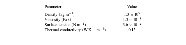
drop-on-demand dispensing system paired with a MicroFab MJ-AT-01-080 nozzle. The droplet volume was estimated from measurements of the dispensed mass and the value of the solvent density, with an estimated error of approximately 10 %, which is likely due to the mass measurement and some solvent evaporation. This solvent was chosen due to its use in the printed-electronics-fabrication experiments that motivated the present work (Cao et al. Reference Cao, Hyun, Francis and Frisbie2020; Nguyen et al. Reference Nguyen, Kumar, Frisbie and Francis2024), and some important physical properties are given in table 1. The substrate rests on a heating plate (Corning PC-420D) whose temperature can be varied, and a microscope and camera (Hirox KH-7700) are used to view the droplet from the top. Image processing software (ImageJ) is used to extract the droplet radius as a function of time. A drop shape analyser (Kruss DSA30S) is used to measure the static contact angle (a 7 μl droplet of 1,2-dichlorobenzene on a UV-cured NOA73 resin substrate), which is
 $10.5^\circ \pm 0.6 ^\circ$
. We note that since the thermal conductivity of NOA73 is 0.17 W
 $\textrm {K}^{-1}\,\textrm {m}^{-1}$
and is similar to that of 1,2-dichlorobenzene (table 1), thermal Marangoni flows may be important in the experiments (Ristenpart et al. Reference Ristenpart, Kim, Domingues, Wan and Stone2007).
Physical properties of 1,2-dichlorobenzene at 25
 $^{\circ }$
C.

(a) Scanning electron micrograph of the mesa (scale bar = 5 μm). Due to the large mesa width, only approximately one-third of the mesa is shown. A layer of silver deposited on the mesa helps outline its shape, but the silver was not used in the experiments reported here. The image background has been processed to improve contrast. (b) Schematic of experimental apparatus.

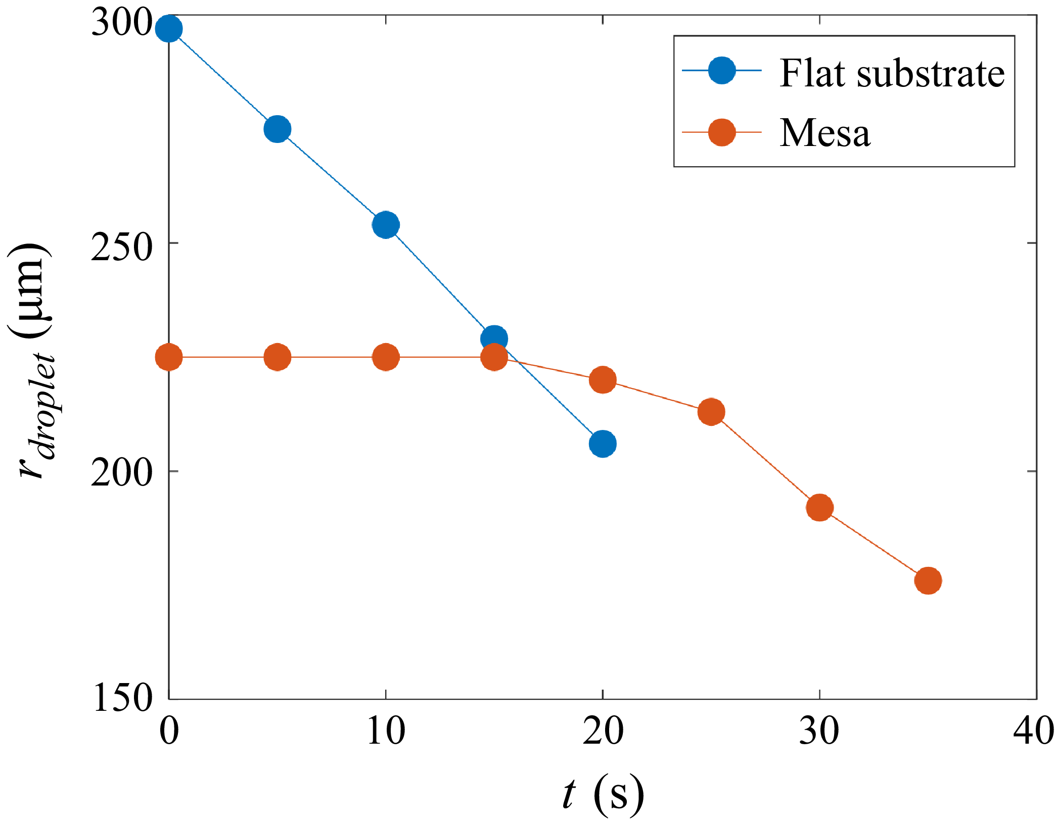
Figure 2 shows typical evolution of the droplet radius (
 $r_{\textit{droplet}}$
) as a function of time (
 $t$
) at a given substrate temperature (
 $T_{b}$
) and initial droplet volume for substrates with and without a mesa. The initial radius is smaller when the mesa is present since the droplet contact line pins at the mesa edge, preventing further spreading. For a flat substrate, the droplet radius decreases monotonically with time, suggesting that contact-line pinning plays a negligible role during the early stages of evaporation on the flat substrate used here. In contrast, for the mesa case, the contact line is pinned at the mesa edge for a significant amount of time before solvent evaporation causes it to depin and retract. Results of other runs under the same conditions are qualitatively similar, with quantitative differences likely arising due to differences in the initial droplet volume (
 $\sim$
10 % as noted above). The measurement error of the droplet radius based on some calibration measurements is estimated to be approximately 0.4 %. We note that after a certain time, the droplet loses axisymmetry and there is no longer a well-defined radius for both the flat-substrate and mesa cases. We believe that the loss of axisymmetry is due to pinning of the droplet contact line on the substrate, which is more likely to happen during the later stages of evaporation when the droplet has significantly thinned.
Plots of
 $r_{\textit{droplet}}$
versus
 $t$
for different substrates when
 $T_{b}=23\,^\circ$
C and the initial liquid volume is 1.98 nl. Data are only shown to the time where the droplet is nearly axisymmetric. After this time, the droplet contact line is no longer nearly circular.

Figure 3 shows typical droplet behaviour for different initial liquid volumes and substrate temperatures. Larger initial volumes (figure 3 a) and lower substrate temperatures (figure 3 b) lead to longer pinning times. Note that, as expected, larger initial droplet volumes and lower substrate temperatures (which correspond to a lower evaporation rate) lead to longer droplet lifetimes. Although it is not the objective of this work to provide detailed quantitative predictions of these experiments, we will see that the lubrication-theory-based model developed in this paper is able to qualitatively describe the behaviour observed in figures 2 and 3.
Plots of
 $r_{\textit{droplet}}$
versus
 $t$
for (a) different initial liquid volumes when
 $T_{b}=23\,^\circ$
C and (b) different
 $T_{b}$
when the initial liquid volume is 1.98 nl.

3. Mathematical model
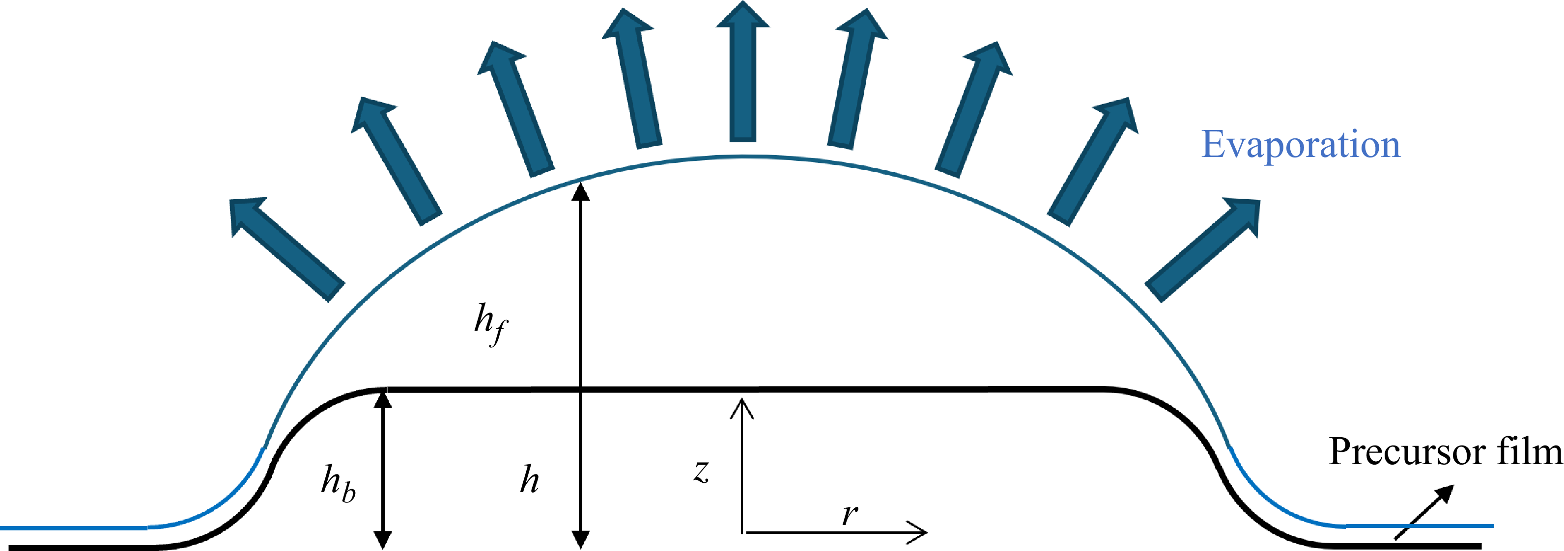
A schematic of the problem geometry is shown in figure 4. We consider an axisymmetric droplet with characteristic height
 $h_{c}$
and characteristic diameter
 $l_{c}$
resting on a mesa with characteristic diameter
 $l_{m}$
and characteristic height
 $h_{m}$
. Because we are interested in thin droplets resting on short mesas, we assume that
 $h_{c} \ll l_{c}$
,
 $h_{m} \ll l_{m}$
and
 $l_{m} \sim l_{c}$
at least. The radial and vertical coordinates,
 $r$
and
 $z$
, are non-dimensionalised by
 $l_{c}$
and
 $h_{c}$
, respectively. The dimensionless liquid–air interface height, film thickness and substrate height (all scaled by
 $h_{c}$
) are denoted
 $h(r,t)$
,
 $h_{\kern-1pt f}(r,t)$
and
 $h_{b}(r)$
, with
 $h_{\kern-1pt f}=h-h_{b}$
. A precursor film is assumed to be present at the droplet edge, and the entire substrate is assumed to be held at a dimensional temperature
 $T_{b}$
.
Schematic of problem geometry.

We consider mesas that are rounded at their edges, such that
 \begin{align} h_{b}=-\frac {m_{h}}{2}\mbox{tanh}\left (m_{s}\left (r-\frac {m_{d}}{2}\right )\right )-\frac {m_{h}}{2}, \end{align}
where
 $m_{h}$
,
 $m_{s}$
and
 $m_{d}$
are dimensionless parameters that control mesa height, steepness and diameter, respectively. Increasing
 $m_{s}$
makes the mesa wall steeper. In our calculations, we fix
 $m_{s} = 5$
and
 $m_{d} = 4$
for simplicity. For most of our calculations, we fix
 $m_{h} = 0.4$
, although we will present some results illustrating the influence of this parameter.
3.1. Hydrodynamics
We use the capillary time as the characteristic time,
 $t^{*}=\mu l_{c} / \sigma \epsilon ^{3}$
, where
 $\mu$
and
 $\sigma$
are the liquid viscosity and surface tension (assumed constant), with
 $\epsilon \equiv h_{c}/l_{c} \ll 1$
. The characteristic velocity and pressure are
 $u^{*}=l_{c}/t^{*}$
and
 $p^{*}=\sigma \epsilon /l_{c}$
. The dimensionless velocity field in the droplet is
 $\boldsymbol {v}=(u,w)$
, where
 $u$
and
 $w$
are radial and vertical velocities, respectively. Here,
 $u$
and
 $w$
have been non-dimensionalised using
 $u^{*}$
and
 $\epsilon u^{*}$
, respectively.
Under the lubrication approximation, the leading-order momentum and mass conservation equations are
 \begin{align} &\frac {\partial p}{\partial r}= \frac {\partial ^{2}u}{\partial z^{2}} , \\[-12pt] \nonumber \end{align}
 \begin{align} &\frac {\partial p}{\partial z}=0 , \\[-12pt] \nonumber \end{align}
 \begin{align} &\frac {1}{r}\frac {\partial [ru]}{\partial r}+\frac {\partial w}{\partial z}=0. \\[10pt] \nonumber \end{align}
In our simulations, gravitational forces are assumed to be negligible relative to surface-tension forces, which corresponds to small Bond numbers
 $Bo=\rho _{l}gl_{c}^{2}/\sigma$
, where
 $\rho _{l}$
is the liquid density and
 $g$
is the magnitude of the gravitational acceleration. This is consistent with our motivating experiments, where
 $Bo\sim 10^{-2}$
.
At the solid–liquid interface (
 $z=h_{b}(r)$
), we have no-slip and no-penetration boundary conditions:
 \begin{align} u=0,\quad w=0. \end{align}
At the liquid–air interface (
 $y=h(r,t)$
), the tangential and normal stress balances are
 \begin{align} & \frac {\partial u}{\partial z}=0 , \\[-12pt] \nonumber \end{align}
 \begin{align} & p-p_{v}=- \frac {\partial ^{2}h}{\partial r^{2}}-\frac {1}{r}\frac {\partial h}{\partial r}-\varPi , \\[10pt] \nonumber \end{align}
where
 $p_{v}$
and
 $\varPi$
are the dimensionless pressure in the vapour phase (assumed constant) and disjoining pressure, respectively. To focus on the influence of the mesa, we neglect any variation of the surface tension with temperature. Based on prior work on a related problem involving droplet evaporation in cavities (Chang & Kumar Reference Chang and Kumar2025), we expect that thermal Marangoni flows will tend to weaken contact-line pinning, as they drive liquid away from the contact line, thereby promoting its retraction. Integrating (3.2) twice and applying the boundary conditions given by (3.5) and (3.6) yields
 \begin{align} u(r,z)=\frac {\partial p}{\partial r}\left (\frac {1}{2}z^{2}-zh-\frac {1}{2}h^{2}_{b}+hh_{b}\right ). \end{align}
3.2. Evaporation
In this work, we use the one-sided model to describe liquid evaporation, where the escape of molecules from the liquid phase to the vapour phase is the rate-limiting step (Ajaev Reference Ajaev2004, Reference Ajaev2005; Sodtke, Ajaev & Stephan Reference Sodtke, Ajaev and Stephan2008; Wilson & D’Ambrosio Reference Wilson and D’Ambrosio2023). This is in contrast to diffusion-limited models, where the evaporation rate is limited by how fast liquid molecules diffuse away from the interface (Hu & Larson Reference Hu and Larson2005; Masoud & Felske Reference Masoud and Felske2009; Larson Reference Larson2014; Wilson & D’Ambrosio Reference Wilson and D’Ambrosio2023). The one-sided model is adopted here for two reasons: (i) the computational cost is lower (only the transport equations in the liquid phase need to be considered) and (ii) the results are often qualitatively similar to predictions from the diffusion-limited model (Murisic & Kondic Reference Murisic and Kondic2008, Reference Murisic and Kondic2011; Larsson & Kumar Reference Larsson and Kumar2023).
In the one-sided model, the expression for the dimensional evaporation flux is
 \begin{align} \frac {\sqrt {2\pi \hat {R}T_{\textit{sat}}}}{\alpha \rho _{v}}j^{\prime }=\frac {p^{\prime }-p_{vap}}{\rho _{l}}+\frac {\hat {L}(T_{i}^{\prime }-T_{\textit{sat}})}{T_{\textit{sat}}}, \end{align}
where
 $\alpha$
,
 $j^{\prime }$
,
 $\hat {R}$
,
 $\hat {L}$
,
 $p^{\prime }$
and
 $T^{\prime }_{i}$
are the accommodation coefficient, evaporation flux, ideal gas constant per unit mass, latent heat of vaporisation per unit mass, pressure at the interface and temperature at the interface, respectively (Ajaev Reference Ajaev2005; Sodtke et al. Reference Sodtke, Ajaev and Stephan2008; Craster, Matar & Sefiane Reference Craster, Matar and Sefiane2009; Wray et al. Reference Wray, Papageorgiou, Craster, Sefiane and Matar2014). (A prime is used here for dimensional variables that will later be non-dimensionalised.) The quantities
 $\rho _{v}$
and
 $\rho _{l}$
are the density of the liquid molecules in the vapour and liquid phases,
 $T_{\textit{sat}}$
is the saturation temperature and
 $p_{vap}$
is the dimensional (constant) pressure in the vapour phase (note that
 $p_{v} \equiv p_{vap}/p^{*}$
). Equation (3.9) indicates that the evaporation flux is proportional to deviations from
 $T_{\textit{sat}}$
or
 $p_{vap}$
. The one-sided model has the form of a mass-transfer coefficient model for the mass flux, so it may provide qualitatively accurate predictions even when its assumptions are not strictly satisfied (Parrish & Kumar Reference Parrish and Kumar2020; Larsson & Kumar Reference Larsson and Kumar2023).
3.3. Energy transport
The temperature in the droplet is scaled as
 \begin{align} T=\frac {T^{\prime }-T_{\textit{sat}}}{T_{b}-T_{\textit{sat}}}=\frac {T^{\prime }-T_{\textit{sat}}}{\Delta T}, \end{align}
where
 $T^{\prime }$
is the dimensional droplet temperature and
 $\Delta T$
is the difference between substrate and saturation temperatures. Because the droplet is thin, the leading-order energy transport equation is
 \begin{align} \frac {\partial ^{2}T}{\partial z^{2}}=0. \end{align}
The dimensional temperature
 $T_{b}$
corresponds to
 \begin{align} T=1\quad \mbox{at } z=h_{b}. \end{align}
When the vapour’s density, viscosity and thermal conductivity are much less than the liquid’s, the conductive heat from the substrate to the liquid–air interface provides the heat of vaporisation. By balancing the conductive heat in the droplet with the heat released through evaporation, we derive the evaporation flux scale:
 \begin{align} j^{*}=\frac {k \Delta T}{h_{c} \hat {L}}, \end{align}
where
 $k$
and
 $\hat {L}$
are the liquid thermal conductivity and latent heat of vaporisation per unit mass. By applying an energy balance at the liquid–air interface, we obtain another boundary condition:
 \begin{align} -\frac {\partial T}{\partial z}=j\quad \mbox{at } z=h, \end{align}
where
 $j$
is the dimensionless evaporation flux.
Solving (3.11) subject to (3.12) and (3.14) yields expressions for the dimensionless evaporation flux and interfacial temperature, which are
 \begin{align} j=\frac {1+\delta (p-p_{v})}{K+h_{\kern-1pt f}},\quad T_{i}=\frac {K-\delta (p-p_{v}) h_{\kern-1pt f}}{K+h_{\kern-1pt f}}, \end{align}
where
 \begin{align} K=\frac {\sqrt {2\pi \hat {R}T_{\textit{sat}}}kT_{\textit{sat}}}{\rho _{v}\alpha \hat {L}^{2}h_{c}},\quad \delta =\frac {\sigma }{\rho _{l} \hat {L}h_{c}}. \end{align}
By applying the kinematic boundary condition at the liquid–air interface, we obtain
 \begin{align} \frac {\partial h}{\partial t}=-\frac {1}{r}\frac {\partial }{\partial r}\left (r \int _{h_{b}}^{h}u\,{\rm d}y \right )-Ej, \end{align}
where
 $E$
is the evaporation number, a ratio between the capillary and evaporation time scales:
 \begin{align} E=\frac {t^{*}}{t_{e}}=\frac {j^{*}}{u^{*}\epsilon \rho _{l}}. \end{align}
By using
 $h_{c}$
,
 $\rho _{l}$
,
 $j^{*}$
and
 $u^*=l_c/t^*$
, we can obtain the evaporation time scale,
 $t_{e}=h_{c}\rho _{l}/j^{*}$
; the capillary time scale
 $t^{*}$
is given in § 3.1. By using (3.8) and (3.15), we can rewrite (3.17) as
 \begin{align} \frac {\partial h}{\partial t}=\frac {1}{r}\frac {\partial }{\partial r}\left ( \frac {\partial p}{\partial r}\frac {rh_{\kern-1pt f}^{3}}{3}\right )-Ej, \end{align}
with
 $p$
given by (3.7). Note that previous studies derive an equivalent equation for evaporation of thin droplets on rough surfaces (Pham & Kumar Reference Pham and Kumar2017, Reference Pham and Kumar2019).
3.4. Disjoining pressure
To model the behaviour of the droplet contact-line region, we assume that a precursor film is present at the droplet edge (figure 4), and use a two-term disjoining pressure including attractive and repulsive interactions:
 \begin{align} \varPi =A_{1} \left [ \left ( \frac {A_{2}}{h_{\kern-1pt f}}\right )^{3}-\left ( \frac {A_{2}}{h_{\kern-1pt f}} \right )^{2} \right ], \end{align}
where
 $A_{1}$
and
 $A_{2}$
are the dimensionless Hamaker constant and precursor-film thickness, respectively. In contrast to tracking the contact line explicitly (Saxton et al. 2016; Savva et al. Reference Savva, Rednikov and Colinet2017), this approach of modelling contact-line motion makes it easier to solve the height evolution equation (3.19), and provides results that are qualitatively consistent with experiments (Hocking Reference Hocking1995; Alleborn & Raszillier Reference Alleborn and Raszillier2004; Zadražil, Stepanek & Matar Reference Zadražil, Stepanek and Matar2006; Morris Reference Morris2014; Espín & Kumar Reference Espín and Kumar2015; Pham & Kumar Reference Pham and Kumar2017, Reference Pham and Kumar2019; Jambon-Puillet et al. Reference Jambon-Puillet, Carrier, Shahidzadeh, Brutin, Eggers and Bonn2018; Kumar & Charitatos Reference Kumar and Charitatos2022; Chang & Kumar Reference Chang and Kumar2025). The choice of exponents in (3.20) is made for computational convenience and is consistent with previous studies (Alleborn & Raszillier Reference Alleborn and Raszillier2004; Espín & Kumar Reference Espín and Kumar2015; Pham & Kumar Reference Pham and Kumar2017, Reference Pham and Kumar2019; Kumar & Charitatos Reference Kumar and Charitatos2022; Chang & Kumar Reference Chang and Kumar2025). We note that although we do not include the effects of surfactant in this work, a previous study suggests that using a precursor-film/disjoining-pressure approach when surfactants are present may yield predictions that deviate significantly from experimental observations since surfactant can flow from the droplet into the precursor film (Van Gaalen et al. Reference Van Gaalen, Diddens, Wijshoff and Kuerten2020).
When the droplet reaches equilibrium on a perfectly flat substrate in the absence of evaporation, the largest angle between the tangent to the liquid–air interface and the substrate is the equilibrium contact angle. Its value in the laboratory frame is denoted as
 $\theta _{e,\textit{lab}}$
. The expression for disjoining pressure, (3.20), can be related to the value of the equilibrium contact angle:
 \begin{align} \theta _{e,\textit{lab}} \approx \epsilon \sqrt {A_{1}A_{2}} \approx \epsilon \theta _{e}, \end{align}
where
 $\theta _{e}$
is the rescaled equilibrium contact angle based on lubrication theory (Schwartz & Eley Reference Schwartz and Eley1998; Schwartz Reference Schwartz1998; Pham & Kumar Reference Pham and Kumar2019). In most of our calculations, we set
 $A_{2}=0.001$
and
 $A_{1}=100$
, which corresponds to a value of
 $\theta _{e}=18.12^\circ$
. In § 7.2, the effects of surface wettability are explored by varying
 $A_{1}$
. In the presence of evaporation, the apparent contact angle will, in general, be time-dependent and differ from the equilibrium value. In the present work, this apparent angle is an output of our numerical calculations. It should be noted that prior studies of droplet evaporation on flat substrates have developed analytical expressions for how the apparent and microscopic contact angles depend on various problem parameters (Morris Reference Morris2001; Savva et al. Reference Savva, Rednikov and Colinet2017; Jambon-Puillet et al. Reference Jambon-Puillet, Carrier, Shahidzadeh, Brutin, Eggers and Bonn2018).
For non-flat substrates, it is useful to define a mesoscopic contact angle,
 $\theta _{\textit{meso}}$
, which is the angle that the droplet–air interface makes with respect to the substrate (Espín & Kumar Reference Espín and Kumar2015; Pham & Kumar Reference Pham and Kumar2017):
 \begin{align} \tan (\theta _{\textit{meso}})=\frac {\frac {\partial h_f}{\partial r}}{1+\frac {\partial h_{b}}{\partial r}\left (\frac {\partial h_f}{\partial r}+\frac {\partial h_{b}}{\partial r}\right )} . \end{align}
The apparent contact angle
 $\theta$
is then taken to be the maximum value of
 $\theta _{\textit{meso}}$
along the interface. The apparent contact-line position,
 $r_{\textit{con}}$
, is the point where the tangent to the liquid–air interface at the maximum value of
 $\theta _{\textit{meso}}$
intersects the substrate. It should be noted that (3.22) is written with respect to the left-hand side of the droplet, where all the derivatives are positive. For the right-hand side of the droplet, all the derivatives are negative and the angle would become negative. In that case, we use the absolute value so we have a positive angle.
To prevent the precursor film from evaporating, the evaporation flux needs to vanish there. By combining this constraint (
 $j=0$
) with (3.7), (3.15) and (3.20), we obtain an expression for the precursor-film thickness with evaporation,
 $\beta$
(Pham & Kumar Reference Pham and Kumar2017; Charitatos, Pham & Kumar Reference Charitatos, Pham and Kumar2021; Chang & Kumar Reference Chang and Kumar2025):
 \begin{align} \beta =-2\sqrt {\frac {\delta A_{1} A^{2}_{2}}{3}} \sinh \left ( \frac {1}{3} \mbox{arcsinh} \left ( -\frac {3A_{2}}{2} \sqrt {\frac {3}{\delta A_{1} A^{2}_{2}}} \right ) \right ). \end{align}
We note that for typical parameter values used in this work (
 $A_1=100$
,
 $A_2=0.001$
and
 $\delta =0.001$
),
 $\beta /A_2 \sim 1$
, so that the precursor film has a comparable thickness in the presence and absence of evaporation.
3.5. Parameter values and numerical methods
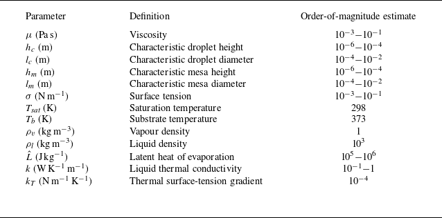
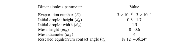
The phenomena reported in § 2 are expected to be quite general, so we consider a broad range of typical values of dimensional parameters, which are listed in table 2. Based on these values, we set
 $\epsilon =0.1$
. Using the values in table 2, we choose a typical capillary time
 $t^{*} \sim 10^{-3}$
s and pick a typical evaporation time
 $t_{e} \sim 10$
s. Based on (3.18),
 $E \sim 10^{-4}$
, a value that has been used in previous studies for droplet evaporation on rough or inclined substrates (Pham & Kumar Reference Pham and Kumar2017, Reference Pham and Kumar2019; Charitatos et al. Reference Charitatos, Pham and Kumar2021). We note that
 $T_{\textit{sat}}$
for 1,2-dichlorobenzene is 452 K at atmospheric pressure (Carswell Reference Carswell1928), which is considerably higher than the value listed in table 2. Although this indicates that the assumptions of the one-sided model are not being satisfied in the experiments reported in § 2, we will see that the relatively simple model we have developed here can qualitatively describe the experimental observations (see also § 3.2). Experiments in which the vapour phase is saturated with the solvent molecules would be expected to be more consistent with the assumptions of the one-sided model.
Order-of-magnitude estimates of dimensional parameters (Burelbach, Bankoff & Davis Reference Burelbach, Bankoff and Davis1988; Vazquez, Alvarez & Navaza Reference Vazquez, Alvarez and Navaza1995; Popescu et al. Reference Popescu, Oshanin, Dietrich and Cazabat2012; Debuisson et al. Reference Debuisson, Merlen, Senez and Arscott2016; Cao et al. Reference Cao, Jochem, Hyun, Francis and Frisbie2018; Nguyen et al. Reference Nguyen, Kumar, Frisbie and Francis2024).

Based on table 2 and (3.16), we estimate
 $K \sim 10^{-1}$
, so we choose
 $K=0.1$
. The accommodation coefficient
 $\alpha$
provides a measure of the ease with which solvent can escape from the liquid to the vapour phase, and we assumed that
 $\alpha \sim 1$
. This is consistent with our previous work involving droplet evaporation in cavities (Chang & Kumar Reference Chang and Kumar2025) and changes to this value are not expected to influence the qualitative behaviour of our results. As in previous studies (Pham & Kumar Reference Pham and Kumar2017; Charitatos et al. Reference Charitatos, Pham and Kumar2021), we choose
 $\delta =0.001$
, which gives a precursor-film thickness (see (3.23)) that is expected to provide qualitatively accurate results at a reasonable computational cost (smaller values of
 $\delta$
lead to smaller values of the precursor-film thickness). Note that smaller values of the precursor-film thickness lead to slower contact-line speeds (for an example, see figure S1 of the supplementary material available at https://doi.org/10.1017/jfm.2026.11733) but are not expected to change the qualitative behaviour of the results (Espín & Kumar Reference Espín and Kumar2017; Chang & Kumar Reference Chang and Kumar2025). The other important dimensionless parameters are listed in table 3.
Dimensionless parameters used for current model.

Although we neglect thermal Marangoni effects to focus on the influence of the mesa (see § 3.1), it is instructive to calculate a thermal Marangoni number:
 \begin{align} Ma_{T}=\frac {k_{T}(T_{b}-T_{\textit{sat}})}{\sigma \epsilon ^{2}}, \end{align}
where
 $k_{T}$
is the thermal surface-tension gradient. Using values from table 1, we estimate that
 $ \textit{Ma}_{T} \sim 1$
, so thermal Marangoni effects may be important in practice. As noted in § 3.1, we expect that these will weaken contact-line pinning, and an example is given in figure S2 of the supplementary material. Nevertheless, we neglect thermal Marangoni effects in this work to isolate the role of the mesa in droplet dynamics. Moreover, while thermal Marangoni effects may produce quantitative changes in the parameter values at which a droplet pins on a mesa (e.g. a steeper mesa slope may be required), we do not expect them to change the qualitative behaviour we observe as different parameters are varied.
We solve the height evolution equation (3.19) on the domain
 $-4\leqslant r \leqslant 4$
by using a fourth-order centred finite-difference scheme and a variable-step, variable-order time-stepping algorithm (Matlab ode15s), with boundary conditions
 $h(-4,t)=h(4,t)=\beta$
and
 $h_{r}(-4,t)=h_{r}(4,t)=0$
. (Note that (3.19) is unchanged when
 $r$
is replaced with
 $-r$
.) We use 2001 spatial nodes, which was found to be sufficient to obtain converged results (see figure S3 of the supplementary material). The model was validated by reproducing previous results for droplet spreading and droplet evaporation on perfectly flat substrates (Tanner Reference Tanner1979; Oron et al. Reference Oron, Davis and Bankoff1997; Pham & Kumar Reference Pham and Kumar2017). (Examples are shown in figures S4 and S5 of the supplementary material.) For the case of no evaporation, we stop the simulation when
 $t=500$
. Each simulation with evaporation is stopped when the maximum film thickness is smaller than
 $1.1 \beta$
(see (3.23)), which means almost all the liquid has dried out. We denote this time as the evaporation time,
 $t_{evap}$
.
Important differences between the experimental conditions and simulation assumptions prevent us from making detailed quantitative comparisons. In the experiments, the mesa walls are nearly vertical since those are easiest to fabricate. Due to the sharp corners this creates where the walls meet the mesa top (radius of curvature
 $\approx$
0.6 μm), the mesa can hold a liquid volume of up to 4 nl before the liquid spills off the mesa. In contrast, our model requires a mesa with rounded corners because it employs the lubrication approximation. Whereas the mesa height and slope are independent for mesas with vertical walls, they are coupled to each other in the mesa model used in our simulations. If we consider a mesa diameter and height of 500 and 5 μm (similar to those of the experiments, but with radius of curvature
 $\approx$
325 μm) at a value of
 $\theta _{e}=18.12^\circ$
, the maximum amount of liquid the mesa can hold is 0.6 nl, which is much smaller than the experimental results. This is consistent with prior work demonstrating that sharp corners are more effective at pinning contact lines than rounded corners (Oliver, Huh & Mason Reference Oliver, Huh and Mason1977). Obtaining quantitatively accurate predictions for mesas with vertical walls will likely require an explicit treatment of the contact-line dynamics (Savva et al. Reference Savva, Rednikov and Colinet2017). In spite of the key differences between experimental conditions and simulation assumptions, we will see that the simulations qualitatively describe the experimental observations reported in figures 2 and 3.
4. No-evaporation case
Before considering the effects of evaporation, we first examine the behaviour of droplets on mesas in the absence of evaporation to highlight some important physical mechanisms. Figure 5(a) shows the initial condition and droplet shape evolution for a representative case. The initial droplet shape is given by a parabolic function:
 \begin{align} h(r,0)=\frac {d_{h}(r-d_{w})^{2}}{d_{w}^{2}}, \end{align}
where droplet height and width are denoted by
 $d_{h}$
and
 $d_{w}$
, respectively. At the droplet edge, the difference between this parabolic function and substrate height is smaller than the precursor-film thickness, so we set
 $h_{\kern-1pt f}=\beta$
there. For simplicity, we choose
 $d_{w}=3$
for our calculations.
Plots of (a)
 $h$
versus
 $r$
at different times and (b)
 $h$
versus
 $r$
at
 $t=500$
. Here,
 $d_{h}=1.7$
,
 $\theta _{e}=18.12^\circ$
and
 $m_{h} = 0.4$
, and the bold dark line is
 $h_{b}$
.

After spreading, the droplet reaches a steady state (
 $t=500$
) shown in figure 5(b), where the contact line is pinned at the mesa edge. Two important variables are also shown that will be helpful in understanding how the mesa influences droplet spreading. The first is
 $\theta _{\textit{max}}$
, which is the apparent contact angle corresponding to the maximum amount of liquid that can be held on the mesa. For the case considered in figure 5, the volume of liquid chosen corresponds to the maximum liquid volume. The second is the substrate inclination angle
 $\phi$
, whose slope (based on scales from lubrication theory) is given by
 \begin{align} \mbox{tan}(\phi )=\max \left ( \frac {{\rm d}h_{b}}{{\rm d}r} \right )=\frac {m_{s}m_{h}}{2}, \end{align}
which ranges from 0.5 to 1.5, with
 $\phi$
ranging from
 $26.57^\circ$
to
 $56.31^\circ$
. For clarity, the mesoscopic contact angle
 $\theta _{\textit{meso}}$
and the apparent contact-line position
 $r_{\textit{con}}$
are also shown in figure 5(b).
The contact-line pinning can be understood by analysing the disjoining and capillary pressure distributions adjacent to the droplet bulk (figure 6 a). The capillary-pressure gradient tends to drive an outward flow, but this is resisted by the disjoining-pressure gradient, which points in the opposite direction. (There are also capillary- and disjoining-pressure gradients adjacent to the precursor film, but the influence of these on the flow is much weaker since the droplet is much thinner there and thus offers greater resistance to flow.) It is instructive to also compare these pressure distributions with those for a droplet of the same volume on a flat substrate when a steady state has been reached (figure 6 b). Again, there is a balance between capillary-pressure gradients and disjoining-pressure gradients at steady state. However, the presence of a mesa causes a larger disjoining-pressure gradient near the droplet edge. This requires a larger capillary-pressure gradient to achieve a steady state, and as a consequence, the capillary pressure in the droplet becomes larger compared with the flat-substrate case.
(a) Pressure distributions for mesa. (b) Pressure distributions for mesa and flat substrate. Here,
 $d_{h}=1.7$
,
 $\theta _{e}=18.12^\circ$
,
 $m_{h}=0.4$
and
 $t=500$
. Because the droplet on the flat substrate has a different steady-state radius, the pressure distributions for that case have been shifted in the
 $-r$
direction for ease of comparison with the mesa.

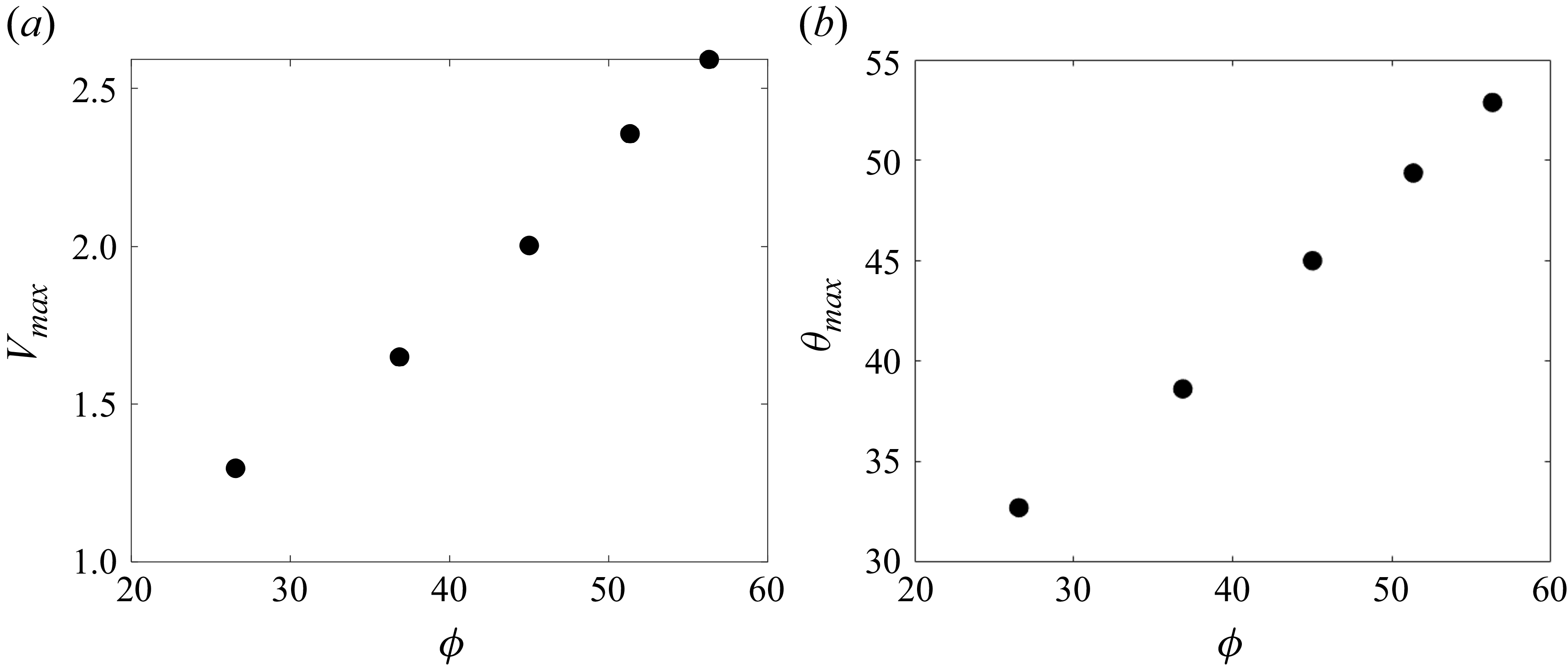
As the inclination angle
 $\phi$
increases, the maximum volume of liquid the mesa can hold,
 $V_{\textit{max}}$
, will increase, as will the apparent contact angle corresponding to this maximum volume,
 $\theta _{\textit{max}}$
(figure 5
b). This behaviour is illustrated in figure 7. To vary
 $\phi$
, we vary
 $m_{h}$
from 0.2 to 0.6. The values of
 $d_{h}$
correspond to those that give the maximum liquid volume the mesa can hold. It should be noted that if the equilibrium contact angle is sufficiently small for a given mesa height, the droplet does not pin at all and simply spreads over the mesa. The results in figure 7 are qualitatively consistent with the Gibbs criterion for a droplet near a sharp corner, where
 $\theta _{\textit{max}}=\theta _{e}+\phi$
(Arogeti & Shapiro Reference Arogeti and Shapiro2024). We would not expect quantitative agreement due to different assumptions used in our calculations including (i) rounded corners, (ii) the presence of a precursor film and disjoining pressure to describe the contact line and (iii) use of the lubrication approximation.
Plots of (a)
 $V_{\textit{max}}$
and (b)
 $\theta _{\textit{max}}$
versus
 $\phi$
when
 $\theta _{e} = 18.12^\circ$
. The values of
 $d_{h}$
(in order of increasing
 $\phi$
) are 1.1, 1.4, 1.7, 2 and 2.2.

5. Influence of initial droplet volume
We now consider the effects of evaporation, focusing in this section on the influence of initial droplet volume. In the simulations, the droplet is first allowed to reach a steady state in the absence of evaporation, then evaporation is turned on.
5.1. Effects of mesa
Figures 8(a) and 8(c) show the time evolution of the contact-line position and the corresponding apparent contact angle in the presence of a mesa for three different initial liquid volumes (set by the initial droplet height,
 $d_{h}$
) at a given evaporation rate. Here, time is rescaled by the evaporation time,
 $t_{evap}$
. Three distinct stages can be observed. In stage 1, the contact line is apparently pinned at the mesa edge for a significant portion of the evaporation time, while the contact angle decreases. In stage 2, the contact line recedes, and the apparent contact angle remains nearly constant. The apparent contact angle in this stage is denoted as
 $\theta _{\textit{CCAS}}$
. From figure 8(c), we see that
 $\theta _{\textit{CCAS}}$
is not sensitive to the initial liquid volume and remains around
 $20^\circ$
. Stage 3 begins when the droplet has nearly evaporated, and here both the contact angle and the contact-line position decrease quickly. These three stages have also been observed in experiments, and in numerical simulations where substrate roughness is accounted for (Deegan et al. Reference Deegan, Bakajin, Dupont, Huber, Nagel and Witten2000; Pham & Kumar Reference Pham and Kumar2017).
Plots of
 $r_{\textit{con}}$
and
 $\theta$
versus
 $t/t_{evap}$
for different
 $d_{h}$
when (a,c)
 $m_{h}=0.4$
and (b,d)
 $m_{h}=0$
. The case where the mesa is absent corresponds to
 $m_{h}=0$
. Here,
 $E=3\times 10^{-5}$
and
 $\theta _{e} = 18.12^\circ$
.

Figure 8. Long description
Panel A: A line graph shows the normalized contact radius (r_con) on the vertical axis versus normalized evaporation time (t/tevap) on the horizontal axis. Three lines represent different values of dh (0.8, 1.2, 1.7), with an arrow indicating increasing dh. The lines show a decreasing trend in r_con as t/tevap increases. Panel B: Another line graph shows the normalized contact radius (r_con) on the vertical axis versus normalized evaporation time (t/tevap) on the horizontal axis. Three lines represent different values of dh (0.8, 1.2, 1.7), with an arrow indicating increasing dh. The lines show a decreasing trend in r_con as t/tevap increases. Panel C: A line graph shows the contact angle (θ) on the vertical axis versus normalized evaporation time (t/tevap) on the horizontal axis. Three lines represent different values of dh (0.8, 1.2, 1.7), with an arrow indicating increasing dh. The lines show a decreasing trend in θ as t/tevap increases. Panel D: Another line graph shows the contact angle (θ) on the vertical axis versus normalized evaporation time (t/tevap) on the horizontal axis. Three lines represent different values of dh (0.8, 1.2, 1.7), with an arrow indicating increasing dh. The lines show a trend where θ initially increases and then decreases as t/tevap increases.
Figures 8(b) and 8(d) show the time evolution of the contact-line position and apparent contact angle for the corresponding case of a perfectly flat substrate. In contrast to what is observed in figure 8(a), the droplet retracts without any significant pinning. However, the apparent contact angle remains nearly constant for most of the evaporation time, as seen in figure 8(d). (The increase in
 $\theta$
at early times is due to evaporation being turned on.) Overall, the results of figure 8 demonstrate that introducing a mesa can cause significant contact-line pinning, with all problem parameters the same.
5.2. Mechanism of pinning and depinning
Figure 9(a) shows the contact-line position at different times in the presence and absence of a mesa, which correspond to the yellow lines in figures 8(a) and 8(b), respectively. It is clear that the presence of a mesa can cause contact-line pinning, and the simulation predictions shown in figure 9(a) are qualitatively consistent with the experimental observations shown in figure 2. To better understand the physical mechanism of the pinning, we examine in figure 9(b) the pressure profiles in the droplets at
 $t=2000$
, when the droplet on the mesa is still pinned. In both the presence and absence of a mesa, the pressure monotonically decreases as one moves from the droplet centre to the edge, and this causes an outward flow. The maximum pressure is at the droplet centre and is denoted as
 $p_{\textit{max}}$
. For the conditions shown in figure 9(b), it is larger when the mesa is present. This corresponds to a larger pressure gradient, which produces a large enough outward flow to replenish liquid evaporated in the contact-line region, leading to a pinned contact line.
Plots of (a)
 $r_{\textit{con}}$
versus
 $t$
and (b) pressure distribution at
 $t=2000$
for different
 $m_{h}$
. The case where the mesa is absent corresponds to
 $m_{h}=0$
. Here,
 $E=3\times 10^{-5}$
,
 $\theta _{e} = 18.12^\circ$
and
 $d_{h}=1.7$
.

Figures 10(a) and 10(b) show
 $p_{\textit{max}}$
and the contact-line position at different times in the absence and presence of a mesa, respectively. When the substrate is perfectly flat,
 $p_{\textit{max}}$
is low enough so the contact line retracts without any significant pinning (figure 10
a). While the contact line retracts,
 $p_{\textit{max}}$
grows monotonically due to a more convex interface. In contrast, when the mesa is present, the contact line is nearly pinned for a significant portion of the evaporation time (figure 10
b). (Note that the pinning is not perfect due to the rounded mesa corner in the simulations.) When the pinning occurs, the contact angle decreases (see figure 8
c), reducing
 $p_{\textit{max}}$
(less convex interface). Once
 $p_{\textit{max}}$
is too low to create a sufficient outward flow to replenish the evaporated liquid in the contact-line region, the contact line depins. After depinning, the droplet shrinks, and the interface becomes more convex, eventually leading to an increase in
 $p_{\textit{max}}$
(
 $p_{\textit{max}}\gt p_{\textit{min}}$
in figure 10
b).
Plots of
 $p_{\textit{max}}$
and
 $r_{\textit{con}}$
versus
 $t$
when (a)
 $m_{h}=0$
and (b)
 $m_{h}=0.4$
. The case where the mesa is absent corresponds to
 $m_{h}=0$
. Here,
 $E=3\times 10^{-5}$
,
 $\theta _{e} = 18.12^\circ$
and
 $d_{h}=1.7$
.

5.3. Dependence of pinning on initial droplet volume
To understand how the initial droplet volume influences contact-line pinning, we examine the time evolution of the contact-line position for three different initial liquid volumes in figure 11(a). Our simulations indicate that a larger initial liquid volume extends the droplet pinning time, which is qualitatively consistent with the experimental results in figure 3(a). Note that in the experiments, the contact line is pinned at the mesa edge (
 $r_{\textit{droplet}}=225$
μm in figure 3
a). However, in the simulations, figure 11(a) shows that a larger initial liquid volume makes the initial droplet radius slightly larger. This difference is due to corner sharpness. Compared with experiments, the corner in the simulations is more rounded, so increasing the initial liquid volume makes the droplet spread slightly further in the simulations.
To help explain why increasing the initial liquid volume increases the percentage of the drying time the droplet is pinned (see figure 8
a), we analyse the time evolution of
 $p_{\textit{max}}$
for three different initial liquid volumes in figure 11(b). From this plot, we see that a larger initial liquid volume increases the pressure at the droplet centre when
 $t=0$
due to a more convex interface. A larger
 $p_{\textit{max}}$
results in a larger capillary-pressure gradient and drives more flow to replenish liquid evaporated in the contact-line region, which explains why increasing the initial liquid volume increases the percentage of the drying time the droplet is pinned. Figure 11(b) also indicates that
 $p_{\textit{min}}$
is not very sensitive to the initial liquid volume, an observation that is discussed further in § 6. We note that as the initial droplet volume increases, so does the droplet aspect ratio since the droplet contact line is initially at the mesa edge.
Plots of (a)
 $r_{\textit{con}}$
versus
 $t$
and (b)
 $p_{\textit{max}}$
versus
 $t/t_{evap}$
for different
 $d_{h}$
. Here,
 $E=3\times 10^{-5}$
,
 $\theta _{e} = 18.12^\circ$
and
 $m_{h}=0.4$
.

6. Influence of evaporation rate
In this section, we focus on the influence of the heating temperature. A higher heating temperature induces faster evaporation in our experiments and corresponds to a larger evaporation number
 $E$
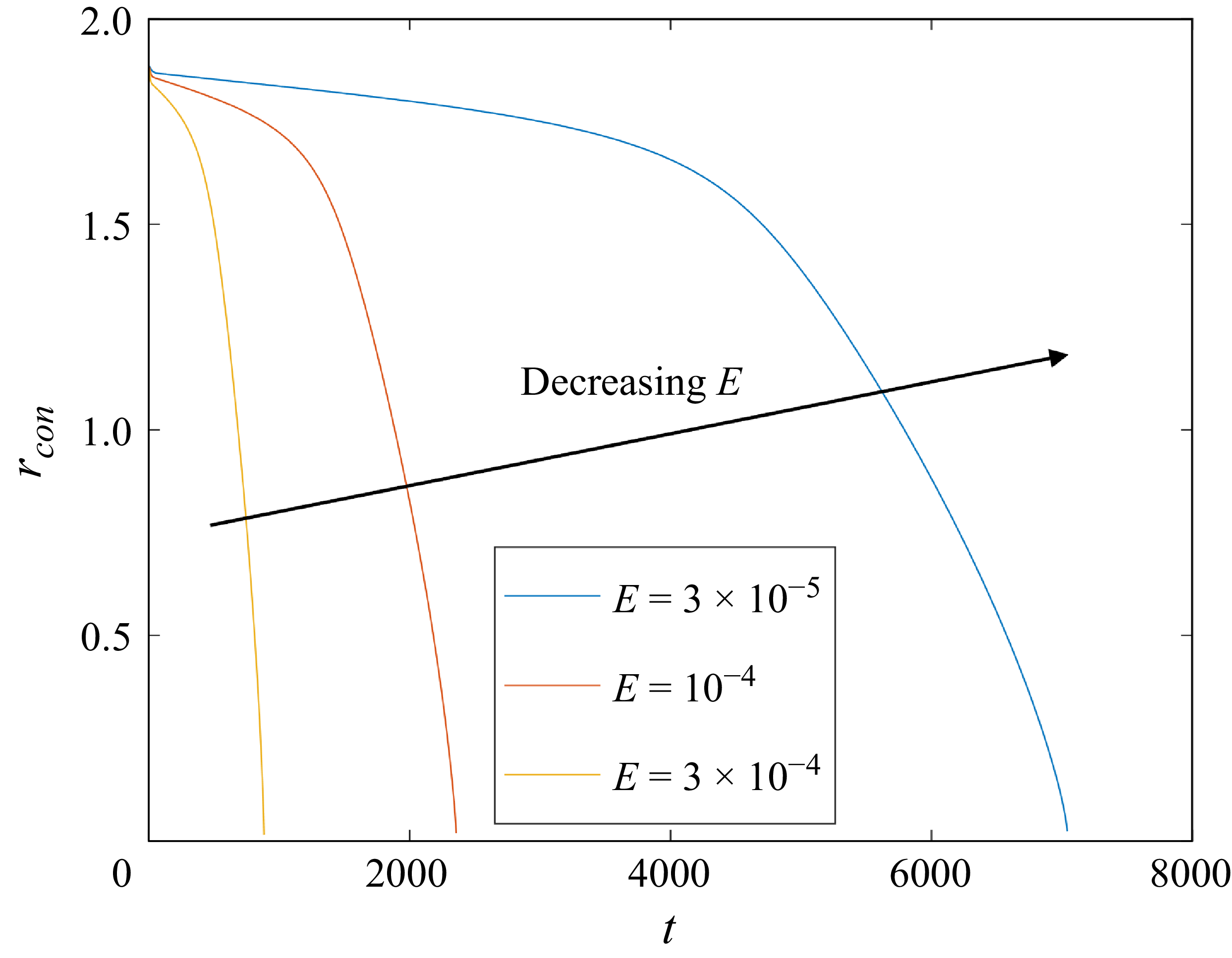
in our simulations (see (3.13) and (3.18)). Figure 12 shows the time evolution of the contact-line position for three different evaporation rates. From this figure, we see that a lower evaporation rate causes longer pinning, which is consistent with the experimental results (see figure 3
b).
Plots of
 $r_{\textit{con}}$
versus
 $t$
for different
 $E$
. Here,
 $d_{h}=1.7$
,
 $\theta _{e} = 18.12^\circ$
and
 $m_{h}=0.4$
.

Figure 13 shows the contact-line position and the corresponding apparent contact angle as a function of
 $t/t_{evap}$
for three different evaporation rates at a given initial liquid volume. In all cases, we observe a three-stage contact-line motion, which was discussed in § 5.1. From figure 13(a), we see that decreasing the evaporation rate slightly increases the percentage of the drying time the droplet is pinned. In contrast to what is observed in figure 8(c), where varying the initial liquid volume does not significantly affect the apparent contact angle in stage 2 (
 $\theta _{\textit{CCAS}}$
), figure 13(b) shows that a lower evaporation rate makes
 $\theta _{\textit{CCAS}}$
smaller, consistent with what is observed on flat substrates (Morris Reference Morris2001; Raj et al. Reference Raj, Kunkelmann, Stephan, Plawsky and Kim2012; Larsson & Kumar Reference Larsson and Kumar2023).
Plots of (a)
 $r_{\textit{con}}$
and (b)
 $\theta$
versus
 $t/t_{evap}$
for different
 $E$
. Here,
 $d_{h}=1.7$
,
 $\theta _{e} = 18.12^\circ$
and
 $m_{h}=0.4$
.

Figure 14(a) shows the time evolution of pressure at the droplet centre (
 $p_{\textit{max}}$
) for three different evaporation rates. Figure 14(a) indicates that slower evaporation makes
 $p_{\textit{min}}$
smaller. It is evident that under slower evaporation, a smaller capillary-pressure gradient is required to drive enough flow to replenish liquid evaporated in the contact-line region, which explains why slower evaporation reduces
 $p_{\textit{min}}$
and thus increases the percentage of the drying time the droplet is pinned. To better understand how evaporation rate affects apparent contact angle, we examine in figure 14(b) the liquid height profile at
 $p_{\textit{max}}=p_{\textit{min}}$
. Note that when
 $p_{\textit{max}}=p_{\textit{min}}$
, the contact line has already depinned. From this figure, we see that at a lower evaporation rate, the contact line depins with a smaller apparent contact angle (
 $\theta _{\textit{CCAS}}$
), corresponding to a lower capillary pressure and smaller capillary-pressure gradient. On the other hand, changing the initial liquid volume cannot affect much the evaporation at the contact-line region. Therefore, the capillary pressure and the resulting capillary-pressure gradient required to make the contact line pinned do not vary much (see figure 11
b), and
 $\theta _{\textit{CCAS}}$
is not sensitive to the initial liquid volume (see figure 8
c).
Plots of (a)
 $p_{\textit{max}}$
versus
 $t/t_{evap}$
and (b)
 $h$
versus
 $r$
at
 $p_{\textit{max}}=p_{\textit{min}}$
for different
 $E$
(the bold dark line is
 $h_{b}$
). Here,
 $d_{h}=1.7$
,
 $\theta _{e} = 18.12^\circ$
and
 $m_{h}=0.4$
.

Plots of (a)
 $r_{\textit{con}}$
and (b)
 $\theta$
versus
 $t$
for different
 $m_{h}$
. Here,
 $d_{h}=0.8$
,
 $\theta _{e} = 18.12^\circ$
and
 $E=3\times 10^{-5}$
.

7. Influence of mesa height and surface wettability
In this section, we focus on the effects of mesa height and surface wettability. By varying the Hamaker constant (
 $A_{1}$
), we can control surface wettability in our simulations (see (3.21)).
7.1. Influence of mesa height
Figure 15 shows the time evolution of the contact-line position and the corresponding apparent contact angle for three different mesa heights. In our simulations, the mesa height (
 $m_{h}$
) ranges from 0.2 to 0.6 so the inclination angle based on lubrication theory varies from
 $26.57^\circ$
to
 $56.31^\circ$
(see (4.2)). In addition, we have reduced the initial droplet height from
 $d_{h}=1.7$
to
 $d_{h}=0.8$
, so the droplet is pinned on the mesa before evaporation begins. Figure 15 indicates that a taller mesa appears to prolong the pinning slightly.
To understand this trend, we examine in figure 16(a) the liquid height profile at
 $t=0$
. This figure reveals that a taller mesa (larger inclination angle) makes initial droplet shape more convex; this is due to a higher disjoining-pressure gradient at the droplet edge (see § 4). The more convex initial shape is consistent with what is observed in figure 15, where the initial radius decreases and the apparent contact angle increases as the mesa becomes taller. Figure 16(b) shows the time evolution of
 $p_{\textit{max}}$
. This figure indicates that increasing mesa height makes
 $p_{\textit{max}}$
larger when
 $t=0$
(more convex interface), so the resulting capillary-pressure gradient and outward flow are larger, corresponding to longer pinning. Note that this mechanism is similar to how the initial liquid volume affects pinning (see § 5.3). It should be noted that because the simulations use mesas with rounded corners, the mesa height influences the mesa slope (see (4.2)). If the mesa sides were perfectly vertical, this would not be the case, so mesa height would not be expected to influence droplet evaporation. In addition, the parameter
 $m_s$
also influences the mesa slope (see (4.2)). Although we do not investigate its effects here, we expect that increasing
 $m_s$
will make more pronounced the influence of mesa height.
Plots of (a)
 $h$
versus
 $r$
at
 $t=0$
and (b)
 $p_{\textit{max}}$
versus
 $t$
for different
 $m_{h}$
. Here,
 $d_{h}=0.8$
,
 $\theta _{e} = 18.12^\circ$
and
 $E=3\times 10^{-5}$
.

7.2. Influence of surface wettability
Figure 17 shows the time evolution of the contact-line position and the corresponding apparent contact angle for three different surface wettabilities. In our simulations, the Hamaker constant (
 $A_{1}$
) ranges from 100 to 400. The rescaled equilibrium contact angle based on lubrication theory varies from
 $18.12^\circ$
to
 $36.24^\circ$
(see (3.21)). In all cases, we observe a three-stage contact-line motion, as discussed in § 5.1. Figure 17 indicates that in stage 2, lower surface wettability causes slower contact-line retraction with a larger apparent contact angle (larger
 $\theta _{\textit{CCAS}}$
). Lower surface wettability makes the apparent contact angle larger, which induces a thicker liquid film at the droplet edge. Therefore, at the droplet edge, evaporation is slower (see (3.15)), which prolongs the drying process. This trend has also been seen in numerical simulations of droplets on flat substrates where substrate roughness is accounted for (Pham & Kumar Reference Pham and Kumar2017).
Plots of (a)
 $r_{con}$
versus
 $t$
at
 $t=0$
and (b)
 $\theta$
versus
 $t$
for different
 $\theta_e$
. Here,
 $d_{h}=1.7$
,
 $m_{h} = 1.4$
and
 $E=3\times 10^{-5}$
.

8. Conclusions
In this paper, we combine flow-visualisation experiments with a lubrication-theory-based model to study droplet evaporation on wide and short mesas. The experiments reveal that the droplet contact line pins at the mesa edge for a significant amount of time, with lower heating temperatures or larger initial liquid volumes further prolonging this pinning.
The lubrication-theory-based model indicates that in the absence of evaporation, the presence of a mesa causes a larger disjoining-pressure gradient near the droplet edge that resists droplet spreading. As the mesa inclination angle increases, so do the maximum volume of liquid the mesa can hold and the corresponding apparent contact angle.
When evaporation is included, compared with the flat-substrate case, the presence of a mesa induces a larger capillary pressure at the droplet centre, which results in a larger capillary-pressure gradient and outward flow, leading to a pinned contact line. Higher heating temperatures enhance evaporation at the droplet edge, shortening the pinning, while larger initial liquid volumes and taller mesas induce more convex droplet profiles and stronger outward flows, extending the pinning duration. Our simulations also reveal changes in the percentage of the total drying time the droplet is pinned when the evaporation rate and initial liquid volume are varied. Lower surface wettability leads to a larger apparent contact angle and prolongs the drying process. While prolonging the pinning time may be useful if one wishes to deposit a uniform layer of a solute (Nguyen et al. Reference Nguyen, Kumar, Frisbie and Francis2024), it also increases the processing time in applications and may promote the coffee-ring effect. The fundamentals uncovered in this work are expected to be useful for optimising the pinning time via choices of the various parameters influencing droplet evaporation on mesas.
Together, our experiments and modelling provide physical insights into how heating temperature, initial liquid volume, mesa height and surface wettability affect droplet evaporation on mesas, which is important for applications such as spray coating (Milionis et al. Reference Milionis, Martiradonna, Anyfantis, Cozzoli, Bayer, Fragouli and Athanassiou2013), microreactors (Kang et al. Reference Kang, Lee, Hwang, Yeon, Lee and Kuh2016; Li et al. Reference Li, Tan, Xiao, Carney, Men, Li, Quon, Ajena, Lam and Pan2018; Song et al. Reference Song, Xu, Xiu and Zhang2020; Fan et al. Reference Fan, Luo, Xu, Song and Zhang2021) and printed-electronics fabrication (Nguyen et al. Reference Nguyen, Kumar, Frisbie and Francis2024). Since the uniformity of particle deposition affects the performance of printed electronics, an important future extension of this work would be to incorporate colloidal suspensions (or other solutes) to explore how droplet pinning impacts deposition patterns. For the lubrication-theory-based model used in this work, this extension is feasible and has already been accomplished in the cases where substrate roughness and cavities are accounted for (Pham & Kumar Reference Pham and Kumar2017; Charitatos et al. Reference Charitatos, Pham and Kumar2021; Chang & Kumar Reference Chang and Kumar2025). Additionally, it may be possible to fabricate mesas with rounded corners (Pal, Sato & Chandra Reference Pal, Sato and Chandra2007; Lorenzini & Morini Reference Lorenzini and Morini2011), which would allow for a closer comparison between theory and experiment. Droplet evaporation in regimes outside the validity of lubrication theory, such as higher equilibrium contact angles and sharper mesa slopes, is also an important open issue and will likely require numerical simulation of the full governing equations. We hope that the present work helps motivate and validate such studies.
Supplementary material
Supplementary material is available at https://doi.org/10.1017/jfm.2026.11733.
Acknowledgements
The authors thank Professor L. Francis for helpful discussions.
Funding
This work was supported by the National Science Foundation (NSF) under Award No. CMMI-2038722. Partial support was also provided by the Coating Process Fundamentals Program of the University of Minnesota.
Declaration of interests
The authors report no conflict of interest.


 ∘

 rdroplet
 t
 Tb=23∘

 rdroplet
 t
 Tb=23∘
 Tb

 h
 r
 h
 r
 t=500
 dh=1.7
 θe=18.12∘
 mh=0.4
 hb

 dh=1.7
 θe=18.12∘
 mh=0.4
 t=500
 −r
 Vmax
 θmax
 ϕ
 θe=18.12∘
 dh
 ϕ

 rcon
 θ
 t/tevap
 dh
 mh=0.4
 mh=0
 mh=0
 E=3×10⁻⁵
 θe=18.12∘

 rcon
 t
 t=2000
 mh
 mh=0
 E=3×10⁻⁵
 θe=18.12∘
 dh=1.7

 pmax
 rcon
 t
 mh=0
 mh=0.4
 mh=0
 E=3×10⁻⁵
 θe=18.12∘
 dh=1.7

 rcon
 t
 pmax
 t/tevap
 dh
 E=3×10⁻⁵
 θe=18.12∘
 mh=0.4
 rcon
 t
 E
 dh=1.7
 θe=18.12∘
 mh=0.4

 rcon
 θ
 t/tevap
 E
 dh=1.7
 θe=18.12∘
 mh=0.4

 pmax
 t/tevap
 h
 r
 pmax=pmin
 E
 hb
 dh=1.7
 θe=18.12∘
 mh=0.4

 rcon
 θ
 t
 mh
 dh=0.8
 θe=18.12∘
 E=3×10⁻⁵

 h
 r
 t=0
 pmax
 t
 mh
 dh=0.8
 θe=18.12∘
 E=3×10⁻⁵

 rcon
 t
 t=0
 θ
 t
 θe
 dh=1.7
 mh=1.4
 E=3×10⁻⁵


 Open access

