1. Introduction
The tear film is a delicate protective layer that helps in the lubrication of the cornea, hydration, cleaning, and defence by trapping and removing debris and bacteria (Fatt & Weissman Reference Fatt and Weissman1992; Sharma, Khanna & Reiter Reference Sharma, Khanna and Reiter1999; Braun Reference Braun2012; Hodges & Dartt Reference Hodges and Dartt2013). In winter, when temperatures are substantially lower, even individuals with healthy eyes may experience dry eye due to tear-film rupture, while those already affected by dry eye syndrome often suffer a worsening of their condition. In fact, the authors’ own experience of dry eyes during the winter season motivated us to solve this problem. This experience posed the following questions. Does ambient air temperature affect tear-film dynamics? Can we explain dry eye symptoms based on the fluid mechanical aspects of the tear film? The present study is aimed at answering these questions.
The tear film is made up of various proteins and biomolecules produced by basal epithelial cells, along with meibomian and lacrimal glands, which act as a barrier against environmental influences and pathogens (Mantelli & Argueso Reference Mantelli and Argueso2008; Braun Reference Braun2012; Dey et al. Reference Dey, Vivek, Dixit, Richhariya and Feng2020). The human tear film can be considered to consist of two layers over the corneal surface: an innermost mucus layer on the corneal epithelium (0.2–0.5 μm in thickness) with a high concentration of mucin molecules that continues into an aqueous layer (4–10 μm) that forms the bulk of the tear film with a low concentration of mucins, and an outermost lipid layer (0.02–1 μm) that faces the environment (Braun Reference Braun2012; Dey et al. Reference Dey, Vivek, Dixit, Richhariya and Feng2020). Note that some studies on tear-film dynamics considered the mucus and aqueous layers as two distinct layers (Sharma & Ruckenstein Reference Sharma and Ruckenstein1986; Zhang et al. Reference Zhang, Craster and Matar2003a , Reference Zhang, Matar and Craster2004). However, as noted by Dey et al. (Reference Dey, Vivek, Dixit, Richhariya and Feng2020), clinical observations imply a continuous variation of the mucin concentration in the mucus and aqueous layers, with the former exhibiting a higher mucin concentration than the latter. Thus, we consider a single layer composed of the mucus and aqueous layers, while the lipid layer is treated as a surfactant layer. Owing to the presence of mucins throughout the film, we consider the tear film as a viscoelastic fluid modelled by the Jeffrey model (Bird, Armstrong & Hassager Reference Bird, Armstrong and Hassager1977).
The lipid layer comprises polar lipids acting as surfactants, which decrease the air–film interface tension (Bron et al. Reference Bron, Tiffany, Gouveia, Yokoi and Voon2004). This leads to solutal Marangoni effects, which drive the particles in the lipid layer after a blink and also stabilise the tear film (King-Smith et al. Reference King-Smith, Fink, Nichols, Nichols, Braun and McFadden2009). When local thinning takes place due to instability, the lipid concentration decreases (higher surface tension) at that location compared with the surrounding region of higher lipid concentration (lower surface tension). The flow occurs from lower to higher surface tension regions, thereby carrying lipid molecules with the flow. This transport then decreases the surface tension of the thinning region, which eventually results in the suppression of the instability. Thus, solutal Marangoni flow helps in stabilising the tear film (Lin & Brenner Reference Lin and Brenner1982; Sharma & Ruckenstein Reference Sharma and Ruckenstein1984, Reference Sharma and Ruckenstein1986; Zhang et al. Reference Zhang, Craster and Matar2003a ,Reference Zhang, Matar and Craster b ; Zhang, Matar & Craster Reference Zhang, Matar and Craster2004; Dey et al. Reference Dey, Vivek, Dixit, Richhariya and Feng2020).
Additionally, the lipid layer forms a coating on the tear film, which reduces evaporation, thereby enhancing the stability of the tear film (Braun Reference Braun2012; Cwiklik Reference Cwiklik2016; Taranchuk & Braun Reference Taranchuk and Braun2024). King-Smith et al. (Reference King-Smith, Fink, Nichols, Nichols, Braun and McFadden2009) presented the mechanisms of tear-film breakup and proposed a three-way classification: immediate, lid-associated and evaporative. The evaporative breakup is probably the most common cause when other types are not evident. The spatial variation in film thickness enhances the elevated local evaporation. Evaporative thinning of the tear film leads to the dehydration of the cornea, and the formation of black streaks (line) and spot (circular) patterns in the human tear film during an inter-blink interval (Peng et al. Reference Peng, Cerretani, Braun and Radke2014; Chen, Driscoll & Braun Reference Chen, Driscoll and Braun2024). Peng et al. (Reference Peng, Cerretani, Braun and Radke2014) demonstrated that tear-film breakup due to evaporation can occur under normal conditions, but only at higher aqueous evaporation rates. Here, ‘normal conditions’ imply ambient temperature, humidity and airflow typical of everyday life, with an intact lipid layer and usual tear-film dynamics. They also analysed the effects of environmental factors such as wind speed and relative humidity on tear-film stability. Higher wind speeds reduce mass transfer resistance, increase the evaporation rate and shorten the rupture time. Lower air humidity aggravates dry eye syndrome by accelerating evaporation and shortening rupture time (McCulley et al. Reference McCulley, Aronowicz, Uchiyama, Shine and Butovich2006). Zhong, Ketelaar & Braun (Reference Zhong, Ketelaar and Braun2019) explained tear film breakup around the thick areas of lipid (glob) due to evaporation and the solutal Marangoni effect.
The tear film may be subjected to long-range van der Waals forces that induce instability (Sharma & Ruckenstein Reference Sharma and Ruckenstein1984; Sharma et al. Reference Sharma, Khanna and Reiter1999; Dey et al. Reference Dey, Vivek, Dixit, Richhariya and Feng2020). The van der Waals dispersion forces acting on the mucous layer contribute to its destabilisation, ultimately leading to rupture (Sharma & Ruckenstein Reference Sharma and Ruckenstein1984). As hydrophilic liquids, similar to mucus or an aqueous tear film, flow over a hydrophobic epithelium, the no-slip condition may lead to inaccurate predictions (Zhang et al. Reference Zhang, Matar and Craster2003b ). Therefore, Zhang et al. (Reference Zhang, Matar and Craster2003b ) and Dey et al. (Reference Dey, Vivek, Dixit, Richhariya and Feng2020) incorporated a Navier slip condition at the film–cornea interface, which further destabilised the tear film. Dey et al. (Reference Dey, Vivek, Dixit, Richhariya and Feng2020) considered a thin tear film model using a continuous viscosity approach, replacing the distinct mucus and aqueous layers with a single liquid layer characterised by continuous profiles of mucin concentration and viscosity. It was shown that, for the same average viscosity, a more viscous liquid near the ocular surface enhances film stability and extends the breakup time. Sharma & Ruckenstein (1984, Reference Sharma and Ruckenstein1986) considered a bilayer model of the tear film with a separate mucus layer between the aqueous layer and the epithelium. The effect of van der Waals forces on tear-film stability was demonstrated using linear and nonlinear theories, which showed a reduction in tear film rupture time. Roy, Roberts & Simpson (Reference Roy, Roberts and Simpson2002) developed a lubrication-based model for the three-dimensional, thin-film flow of a Newtonian viscous fluid over an arbitrarily curved substrate, which applies to many draining, coating and biological flow scenarios. Using a physical multiple-scale expansion, their model systematically incorporates the substrate’s curvature tensor into the film dynamics and demonstrates a strong impact of substrate curvature on film dynamics. For tear film, Braun et al. (Reference Braun, Usha, McFadden, Driscoll, Cook and King-smith2012) analysed the flow of thin Newtonian and Ellis fluid films on a prolate spheroid to understand the effect of corneal curvature on tear-film dynamics. Their analysis predicted a weak effect of corneal curvature on the thinning rate at the centre of the cornea. Allouche et al. (Reference Allouche, Abderrahmane, Djouadi and Mansouri2017) investigated the influence of curvature on tear-film dynamics and found that, away from the upper eyelid, curvature has a minimal effect on film thickness. Thus, we consider a planar cornea upon which the tear film is situated.
The mucin protein molecules present in the tear film impart elasticity along with high viscosity and shear-thinning. However, previous analyses neglected tear-film elasticity while considering shear-thinning (Zhang et al. Reference Zhang, Craster and Matar2003a ). Thus, in the present analysis, we treat the tear film as a viscoelastic fluid. Previous analyses have shown tear-film destabilisation and eventual rupture due to van der Waals forces and evaporation, along with lid-associated rupture. Here, we demonstrate that there is yet another hitherto unreported thermocapillarity route by which the tear film can exhibit instability and rupture. To focus on thermocapillary-induced rupture and make the problem mathematically tractable, we neglect evaporation in the present analysis. As discussed later, this results in the loss of quantitative agreement between our predictions and clinical observations. However, the qualitative picture presented in the present study remains valid, which is also the aim of the present study.
The rest of the paper is arranged as follows. The base state quantities, linearised governing equations and boundary conditions are derived in § 2. The results of the general linear stability analysis (applicable for the whole wavenumber range) are presented and discussed in § 3. The derivation of the longwave evolution equation, and linear and nonlinear stability analyses using the evolution equation are presented in § 4. The summary of the present investigation is given in § 6.
2. Problem formulation
Consider a film of an incompressible viscoelastic liquid with temperature-independent viscosity
 $\mu$
, thermal diffusivity
 $\kappa$
and density
 $\rho$
. The film has a mean thickness
 $d$
and is deposited upon a planar substrate, as shown schematically in figure 1. We consider the tear film of a standing or seated human in the upright position, such that the air–film interface lies parallel to the direction of gravity. The film is exposed to the ambient inert air at
 $y^*=d$
and the film–substrate interface is located at
 $y^*=0$
, where superscript
 $^*$
denotes a dimensional quantity that will be non-dimensionalised later. The film–air interface is assumed to be a deformable surface with temperature-dependent surface tension
 $\sigma ^*$
.
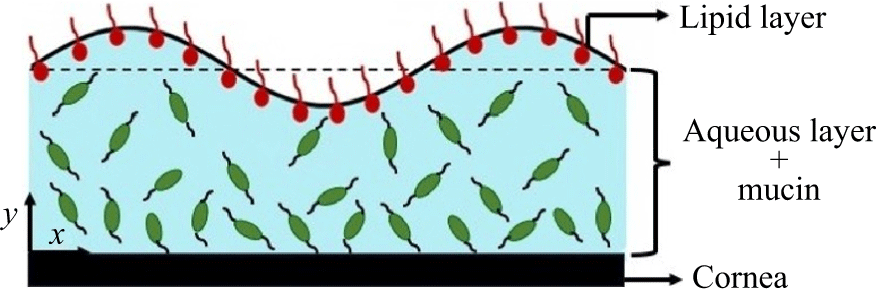
Schematic of the tear-film structure considered in the present study. The wave shown at the air–film interface is due to perturbations imposed on the mean interface
 $y=1$
(in dimensionless scale). The cornea–film interface is located at
 $y=0$
. As shown, mucin concentration decreases along the positive y-axis, leading to a decrease in viscosity and elasticity with increasing film height.

The ambient air and the substrate are maintained at uniform temperatures
 $T^\ast _\infty$
and
 $T^\ast _0$
, respectively. Thus, the layer is subjected to a temperature difference
 $\Delta T^\ast =T^\ast _0 - T^\ast _\infty$
. Owing to the small thickness of the tear film (
 $\sim O(10^{-6}\text{m})$
), the buoyancy effect is neglected. Following the previous studies of Braun (Reference Braun2012) and Zhang et al. (Reference Zhang, Craster and Matar2003a
,
Reference Zhang, Matar and Crasterb
, Reference Zhang, Matar and Craster2004), to understand the role of the lipid layer on the tear film, we consider an insoluble surfactant at the air–film interface. The surface tension
 $\sigma ^*$
is assumed to be a linearly decreasing function of temperature (
 $T^*$
) and surfactant concentration (
 $\varGamma ^*$
) as
 $\sigma ^*=\sigma ^*_0-\alpha _T^* (T^*-T^*_0) - \alpha _\varGamma ^* (\varGamma ^*-\varGamma _0)$
, where
 $\alpha _T^*=-{\text{d}\sigma ^*}/{\text{d}T^*}\gt 0$
and
 $\alpha _\varGamma ^*=-{\text{d}\sigma ^*}/{\text{d}\varGamma ^*}\gt 0$
. The interface tension
 $\sigma ^*_0$
is evaluated at the reference temperature
 $T^*_0$
and
 $\varGamma _0$
. Here, we use the Cartesian coordinate system with the axes
 $x^\ast$
and
 $z^\ast$
located in the substrate plane, and
 $y^\ast$
normal to the substrate.
To account for the mucus layer (formed by mucins) located just above the cornea, Sharma & Ruckenstein (Reference Sharma and Ruckenstein1986) and Zhang et al. (Reference Zhang, Craster and Matar2003a
,
Reference Zhang, Matar and Crasterb
, Reference Zhang, Matar and Craster2004) considered a two-layer model involving a highly viscous mucin layer near the cornea and a lower viscosity aqueous layer on the mucin layer. This model assumed a sharp interface separating the aqueous and mucus layers, leading to a finite interfacial tension at the aqueous–mucus layers interface and van der Waals interactions with the other surfaces. However, as noted by Prydal et al. (Reference Prydal, Artal, Woon and Campbell1992), Bron et al. (Reference Bron, Tiffany, Gouveia, Yokoi and Voon2004), Braun (Reference Braun2012) and Dey et al. (Reference Dey, Vivek, Dixit, Richhariya and Feng2020), mucin is found throughout the tear film and forms a continuously varying profile. Also, mucin proteins (the constituent of the mucus layer) are soluble in water, which does not allow a sharp interface between mucin and aqueous layers. Based on these observations, Dey et al. (Reference Dey, Vivek, Dixit, Richhariya and Feng2020) proposed a continuous-viscosity model with the highest viscosity at
 $y=0$
and the lowest viscosity at
 $y=1$
(see figure 1). Further, they assumed viscosity to be proportional to mucin concentration with a known mucin concentration profile. While they considered linear and hyperbolic tangent mucin concentration profiles, here we consider a linear profile to obtain an analytical solution for the longwave evolution equation.
Following Dey et al. (Reference Dey, Vivek, Dixit, Richhariya and Feng2020), we assume viscosity to be proportional to mucin concentration. This implies that the tear-film viscosity (
 $\mu ^*$
) linearly decreases with increasing
 $y$
such that
 $\mu ^* = \mu _0 (\mu _r - (\mu _r-1) y^*/d)$
. Here,
 $\mu _0$
is the viscosity of the mucus layer at
 $y^*=d$
and
 $\mu _r$
is the ratio of viscosity at
 $y^*=0$
to
 $\mu _0$
. Note that a linear viscosity profile allows us to obtain an analytical solution for the longwave evolution equation; thus, the assumption of a linear viscosity profile. Additionally, the relaxation time
 $\lambda _1^* = \mu ^*/G$
, where
 $G$
is the constant shear modulus of the tear film; thus,
 $\lambda _1^* = \mu _0/G \, (\mu _r - (\mu _r-1) y^*/d)$
. Note that, as stated in § 1, we have neglected evaporation owing to the mathematical complexity. However, evaporation could become the central mechanism in tear-film thinning and breakup, particularly under low-humidity or high airflow conditions. As discussed later in § 4.3, tear film rupture thermocapillarity can become important when the ambient air temperature is substantially lower than the cornea temperature.
The length, velocity, time, surfactant concentration, viscosity, relaxation time and temperature are scaled by
 $d, \kappa /d$
,
 $d^2/\kappa$
,
 $\varGamma _0$
,
 $\mu _0$
,
 $\mu _0/G$
and
 $\beta d$
, respectively, where
 $\beta =-{\text{d}\bar T^*}/{\text{d}y^*}$
is the imposed temperature gradient and the overbar denotes a base state quantity. Furthermore, pressure and stresses are scaled by
 $\mu _0 \kappa /d^2$
. Let the scaled velocity, pressure and stress fields be denoted by
 $\boldsymbol{v} = (v_x, v_y, v_z)$
,
 $p$
and
 $\boldsymbol{\tau }$
, respectively. The scaled continuity, momentum conservation and heat advection–diffusion equations are
 \begin{align} \boldsymbol{\nabla }\boldsymbol{\cdot }\boldsymbol{v}=0, \\[-28pt] \nonumber \end{align}
 \begin{align} \frac {1}{Pr} \left [ \frac {\partial \boldsymbol{v}}{\partial t} + (\boldsymbol{v} \boldsymbol{\cdot }\boldsymbol{\nabla }) \boldsymbol{v} \right ] =- \boldsymbol{\nabla }p + \boldsymbol{\nabla }\boldsymbol{\cdot }\boldsymbol{\tau }, \\[-28pt] \nonumber \end{align}
 \begin{align} \frac {\partial T}{\partial t}+(\boldsymbol{v}\boldsymbol{\cdot }\boldsymbol{\nabla }) \, T = \boldsymbol{\nabla} ^{2} T, \\[0pt] \nonumber \end{align}
where
 $\displaystyle Pr={\mu }/{\rho \kappa }$
is the Prandtl number,
 $\displaystyle \boldsymbol{\nabla }= ( {\partial }/{\partial x},{\partial }/{\partial y},{\partial }/{\partial z} )$
is the gradient operator and
 $\displaystyle \boldsymbol{\nabla} ^2 \equiv {\partial ^2}/{\partial x^2}+ {\partial ^2}/{\partial y^2}+ {\partial ^2}/{\partial z^2}$
is the Laplacian operator. Owing to these scales,
 $\mu =\mu _r - (\mu _r-1) y$
and
 $\lambda =\mu _r - (\mu _r-1) y$
, where
 $\mu =\mu ^*/\mu _0$
and
 $\lambda =\lambda ^* G/\mu _0$
. To describe the dynamics of the tear film, we use the Jeffreys model owing to the viscoelastic nature of the tear film (Bird et al. Reference Bird, Armstrong and Hassager1977),
 \begin{eqnarray} \left [ 1+L_1 \, \mu \, \frac {\partial }{\partial t} \right ] \boldsymbol{\tau }=\mu \, \left [ 1+L_2 \frac {\partial }{\partial t} \right ] \big(\boldsymbol{\nabla }\boldsymbol{v}+\boldsymbol{\nabla }\boldsymbol{v}^T \big), \end{eqnarray}
where
 $\displaystyle L_1=({\mu _0 \kappa }/{G\, d^2})$
and
 $\displaystyle L_2={\lambda ^*_2 \kappa }/{d^2}$
with
 $\lambda ^*_2$
representing the dimensional retardation time.
The governing equations (2.1) are subjected to the following boundary conditions. At
 $y=0$
, following previous studies (Zhang et al. Reference Zhang, Craster and Matar2003a
; Braun Reference Braun2012), we assume slip and impermeability at the substrate. Additionally, the substrate is assumed to be maintained at a constant specified scaled temperature (
 $T_0$
) at
 $y=0$
, implying a constant temperature of the cornea. These assumptions yield
 \begin{eqnarray} v_x=\delta \tau _{xy}, \quad v_y=0, \quad v_z=0, \quad T=T_0, \end{eqnarray}
where
 $\delta$
is the slip parameter. The constant temperature at the cornea–tear film interface is assumed since the body will try to regulate the cornea temperature to maintain its function properly and avoid damage to the cornea by aqueous humour circulation, eyelid protection and conjunctival and limbal circulation (Efron & Young Reference Efron and Young1981; Sweeney & Gressel Reference Sweeney and Gressel1998; Tan et al. Reference Tan2016). Due to this, the cornea temperature is assumed to be the same as the body temperature.
We also consider van der Waals forces acting at the air–film interface (
 $y=1+\xi (x,t)$
) in dimensionless terms as
 $\phi = -A/(1+\xi )^3$
, where
 $\xi$
is the displacement of the interface from its mean position
 $y=1$
and
 $A=A^*/(6 \pi \mu _0 \kappa d)$
is the scaled Hamaker constant with
 $A^*$
as the dimensional Hamaker constant. At the air–film interface, the boundary conditions are the kinematic boundary condition, the tangential and normal stress balances, and the continuity of heat flux respectively
 \begin{align} \frac {\partial \xi }{\partial t} +\boldsymbol{v}_\perp \boldsymbol{\cdot }\boldsymbol{\nabla }\xi = v_y , \\[-28pt] \nonumber \end{align}
 \begin{align} \boldsymbol{t} \boldsymbol{\cdot }\boldsymbol{\tau } \boldsymbol{\cdot }\boldsymbol{n}= - \textit{Ma}_t \boldsymbol{\nabla }T \boldsymbol{\cdot }\boldsymbol{t} - \textit{Ma}_s \boldsymbol{\nabla }\varGamma \boldsymbol{\cdot }\boldsymbol{t}, \\[-28pt] \nonumber \end{align}
 \begin{align} -p - \phi + \boldsymbol{n} \boldsymbol{\cdot }\tau \boldsymbol{\cdot }\boldsymbol{n}=-\frac {1}{\textit{Ca}} (\boldsymbol{\nabla }\boldsymbol{\cdot }\boldsymbol{n}) , \\[-28pt] \nonumber \end{align}
 \begin{align} \boldsymbol{\nabla }T \boldsymbol{\cdot }\boldsymbol{n}=-\textit{Bi} (T-T_\infty ), \\[0pt] \nonumber \end{align}
where
 \begin{eqnarray} \textit{Ma}_t=\frac {\alpha ^*_T \beta d^2}{\mu _0 \kappa },\quad \textit{Ma}_s=\frac {\alpha ^*_\varGamma \varGamma _0^* d}{\mu _0 \kappa },\quad \textit{Bi}=\frac {qd}{k_{th}}, \quad \textit{Ca}=\frac {\mu _0 \kappa }{\sigma ^*_0 d}, \end{eqnarray}
are the thermocapillary Marangoni, solutal Marangoni, Biot and capillary numbers, respectively. Here
 $q$
,
 $k_{th}$
and
 $ \sigma ^*_0$
are the coefficient of thermal convection at the free surface, the thermal conductivity of the fluid, and surface tension evaluated at the free surface temperature and equilibrium surfactant concentration, respectively. The vectors
 $\boldsymbol{n}$
and
 $\boldsymbol{t}$
are the unit normal and tangent vectors to the air–film interface, respectively. Also, the vector
 $\boldsymbol{v}_\perp$
is the two-dimensional part of vector
 $\boldsymbol{v}$
,
 ${\boldsymbol v}_\perp = (v_x,v_y )$
. Notice the absence of a gravity term in the normal stress balance (2.2d
). This is because the air–film interface is parallel to the gravity. The scaled transport equation for the insoluble surfactant is (Zhang et al. Reference Zhang, Craster and Matar2003a
; Braun Reference Braun2012)
 \begin{eqnarray} \frac {\partial \varGamma }{\partial t}+ \frac {\partial }{\partial x} (v_x \varGamma ) = \frac {\kappa _r}{Le}\frac {\partial ^2\varGamma }{\partial x^2}. \end{eqnarray}
Here,
 $\kappa _r = \kappa _s/\kappa$
is the ratio of thermal diffusivity of the surfactant and the film, and
 $Le=\kappa _s/D$
is the Lewis number, with
 $\kappa _s$
and
 $D$
as the thermal and molecular diffusivities of the surfactant.
The governing equations (2.1) and boundary conditions (2.2) yield the dimensionless base state of the system
 \begin{eqnarray} \boldsymbol{\bar v} =0, \quad \bar T=- y+T_0, \quad \bar \varGamma = 1. \end{eqnarray}
To analyse the stability of the tear film, infinitesimally small perturbations are imposed on the base state (2.3). From Patne, Agnon & Oron (Reference Patne, Agnon and Oron2020a), Squire’s theorem is applicable in the present case for a viscoelastic film. Thus, in what follows, following Patne et al. (Reference Patne, Agnon and Oron2020a
), we consider two-dimensional perturbations. The governing equations (2.1) are linearised around the base state (2.3). In the resulting linearised equations, normal modes
 $g'(\boldsymbol{x},t)=\tilde {g}(y) \exp {(i k x +s t)}$
are substituted. Here,
 $g'(\boldsymbol{x},t)$
is the perturbation to a dynamic quantity
 $g (\boldsymbol{x},t )$
and
 $\tilde {g}(y)$
is the corresponding eigenfunction in the Laplace–Fourier space. The parameters
 $k$
and
 $s=s_r+i s_i$
are the wavenumber of the perturbations in the
 $x$
-direction and complex growth rate, respectively. The flow is linearly unstable if at least one eigenvalue satisfies the condition
 $s_r\gt 0$
.
Upon simplification, the governing equations yield
 \begin{align} ik\tilde v_x + D \tilde {v}_y=0, \\[-28pt] \nonumber \end{align}
 \begin{align} \frac {1}{Pr} s \tilde {v}_x =- ik \tilde p + ik \tilde \tau _{xx} + D \tilde \tau _{xy}, \\[-28pt] \nonumber \end{align}
 \begin{align} \frac {1}{Pr} s \tilde {v}_y =- D \tilde p + ik \tilde \tau _{xy} + D \tilde \tau _{yy}, \\[-28pt] \nonumber \end{align}
 \begin{align} s \tilde {T} - \tilde {v}_y= \big(D^2-k^2 \big) \tilde T, \\[-28pt] \nonumber \end{align}
 \begin{align} (1+ \, \mu \, L_1 s)\tilde \tau _{xx}=2ik \, \mu \, (1+L_2 s) \tilde v_x, \\[-28pt] \nonumber \end{align}
 \begin{align} (1+ \, \mu \, L_1 s)\tilde \tau _{xy}=2 \, \mu \, (1+L_2 s) \left ( D\tilde v_x+ik \tilde {v}_y \right ), \\[-28pt] \nonumber \end{align}
 \begin{align} (1+ \, \mu \, L_1 s)\tilde \tau _{yy}=2 \, \mu \, (1+L_2 s) D\tilde v_y. \\[-6pt] \nonumber \end{align}
where
 $ D=\text{d}/\text{d}y$
.
The boundary conditions (2.2) lead to the following set of equations. At
 $y=0$
, the boundary conditions modify to
 \begin{eqnarray} \tilde v_x= \delta \tilde \tau _{xy}, \quad \tilde v_y=0, \quad \tilde T=0. \end{eqnarray}
Similarly, the boundary conditions at the air–film interface yield
 \begin{align} \tilde v_y=s\tilde \xi , \\[-28pt] \nonumber \end{align}
 \begin{align} \tilde \tau _{xy}=-ikMa_t ( \tilde T - \tilde {\xi } ) - ik Ma_s \tilde \varGamma , \\[-28pt] \nonumber \end{align}
 \begin{align} -\tilde p - 3 A \tilde \xi +\tilde \tau _{yy}=-\frac {k^2}{Ca} \tilde \xi , \\[-28pt] \nonumber \end{align}
 \begin{align} D \tilde T + Bi (\tilde T - \tilde \xi )=0. \\[-28pt] \nonumber \end{align}
 \begin{align} s \tilde \varGamma + ik\tilde v_x=-\frac {k^2 \, \kappa _r}{Le} \tilde \varGamma . \\[-6pt] \nonumber \end{align}
The simplified governing equations (2.4) and boundary conditions (2.5) form a generalised linear eigenvalue problem for the eigenvalues
 $s$
and the eigenfunctions for a specified set of parameters. To solve the eigenvalue problem, we employ the pseudo-spectral method, briefly explained in Appendix A.
3. General linear stability analysis (GLSA)
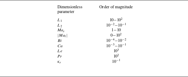
In this section, we will analyse the stability of perturbations over the full range of wavenumbers to determine the wavenumber of the most unstable perturbations. The conclusion obtained from this section will then be used in § 4 to obtain the longwave evolution equation. Using the dimensional parameter ranges discussed in Appendix B, we obtain the ranges of dimensionless parameters. The result of this exercise is provided in table 1. For the present analysis, we will fix
 $ \textit{Pr}=100, Le=1000, Bi=0.001$
and
 $\kappa _r=0.1$
for the rest of the analysis. In the subsequent discussion, we investigate the effect of tear-film elasticity, solutocapillarity due to the lipid layer (surfactant), capillarity, slip at the substrate and thermocapillarity on the stability of the tear film.
Order of magnitude of the dimensionless parameters using the dimensional parameters. Note that
 $ \textit{Ma}_t\gt 0$
, if the ambient air temperature is lower than the corneal temperature and vice versa. Highest value of
 $ \textit{Ma}_s\approx 30$
.

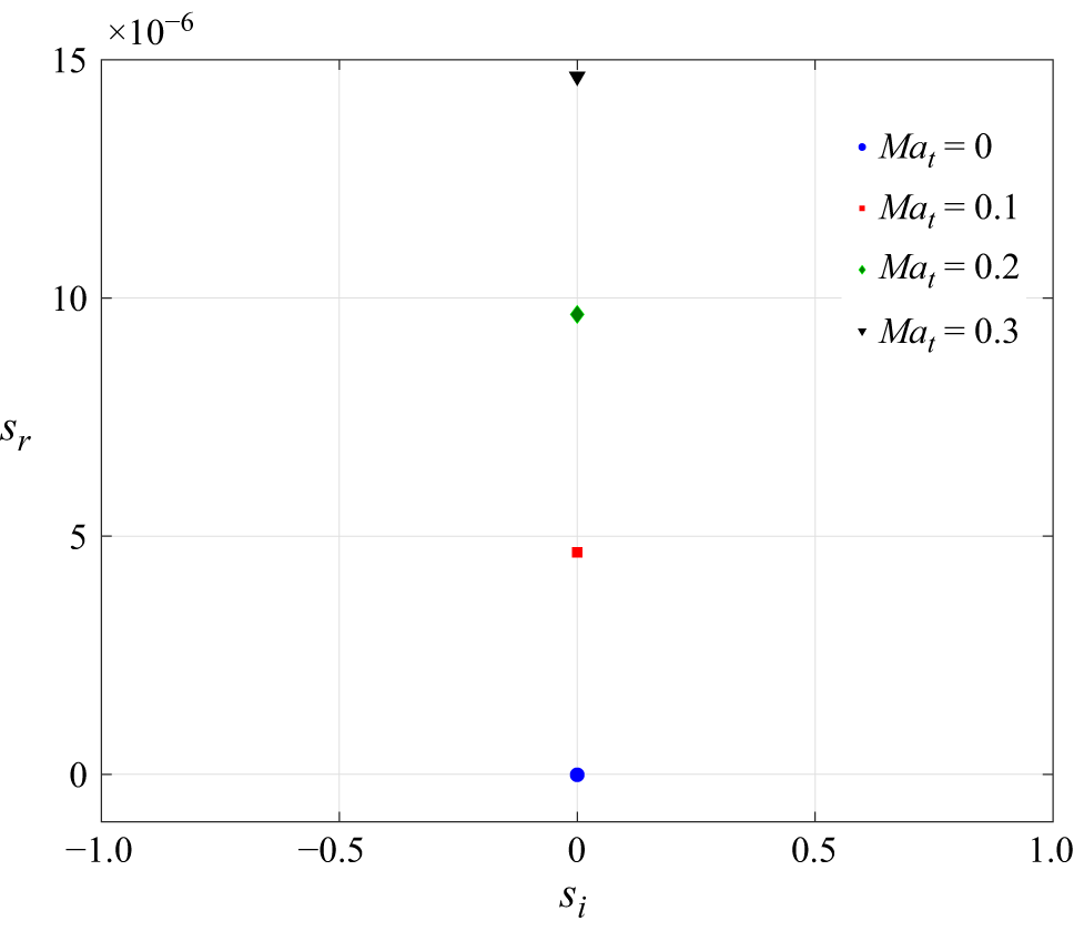
Movement of the unstable (least stable) eigenvalue in
 $s_i{ - }s_r$
space due to an increasing thermocapillary Marangoni number for
 $ \textit{Bi}=10^{-3},k=0.01,L_1=0,L_2=0,Ma_s=0, \mu _r=1, A=0$
and
 $ \textit{Ca}=0.01$
. The film is unstable for
 $ \textit{Ma}_t\gt 0$
.

Figure 2 demonstrates the effect of thermocapillarity on film stability in the absence of surfactant, wall slip and film elasticity. Clearly, the film becomes unstable for
 $ \textit{Ma}_t \gt 0$
, which implies that when the ambient temperature is lower than the corneal temperature, the film is unstable. Moreover, the presence of instability for low wavenumbers indicates the longwave nature of the instability. The absence of a critical Marangoni number (
 $ \textit{Ma}_{tc}$
) required to destabilise the film can be understood as follows.
For a thin film heated from below and air–film interface perpendicular to gravity,
 $ \textit{Ma}_{tc} = ({2 (1+Bi)Bo}/{3 Ca})$
, where
 $ \textit{Bo}= {\rho g d^2}/{\sigma ^*}$
is the Bond number (Oron, Davis & Bankoff Reference Oron, Davis and Bankoff1997; Patne, Agnon & Oron 2021a). The Bond number enters through the normal stress balance at the air–film interface. For a standing or sitting human being, the air–film interface is parallel to gravity, provided that the corneal curvature is neglected. Previous studies indicate that the corneal curvature can indeed be neglected owing to the extremely small thickness of the tear film and the relatively large radius of corneal curvature (Braun Reference Braun2012; Braun et al. Reference Braun, Usha, McFadden, Driscoll, Cook and King-smith2012). Owing to this, the Bond number becomes irrelevant in the present study. This leads to
 $ \textit{Ma}_{tc}=0$
, thereby justifying the results shown in figure 2.
3.1. Effect of lipid layer (
 $ \textit{Ma}_s \neq 0$
)

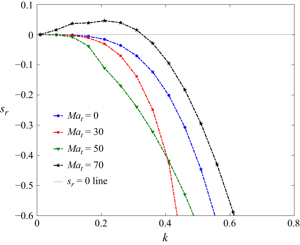
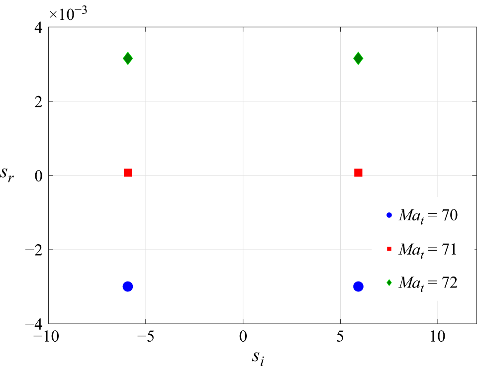
Effect of variation in the thermocapillary Marangoni number
 $ \textit{Ma}_t$
on the stability of the tear film for
 $L_1=0,L_2=0,Ma_s=30,\delta =0, \mu _r=1, A=0$
and
 $ \textit{Ca}=0.01$
. Only the most unstable mode is shown for
 $ \textit{Ma}_t=70$
. There is one more unstable mode with a lower
 $s_r$
value, as discussed in the text. Here, the critical
 $ \textit{Ma}_t=60$
.

Previous studies by Zhang et al. (Reference Zhang, Craster and Matar2003a
,
Reference Zhang, Matar and Crasterb
), Braun (Reference Braun2012) and Dey et al. (Reference Dey, Vivek, Dixit, Richhariya and Feng2020) indicate that the solutocapillarity effect due to the lipid layer is the major stabilising factor for the tear film. This leads to the following question. Can thermocapillarity destabilise the tear film by overcoming the stabilising effect of the lipid layer? Thus, we next consider the highest value possible for the tear-film solutal Marangoni number, i.e.
 $ \textit{Ma}_s \approx 30$
, and increase the thermocapillary Marangoni number as shown in figure 3. For
 $ \textit{Ma}_t=70$
, the dispersion curve exhibits an unstable zone and the film becomes unstable. The dispersion curves for select values of
 $ \textit{Ma}_t$
are shown in figure 3. The value
 $ \textit{Ma}_t=70$
is well within the realistic values. Thus, the tear film can break up due to thermocapillary-induced instability.
Contour plot showing the isocontours of thermal perturbations for
 $L_1=0,L_2=0,Ma_s=10, \delta =0, Ma_t=20.1, \mu _r=1, A=0, k=0.01$
and
 $ \textit{Ca}=0.01$
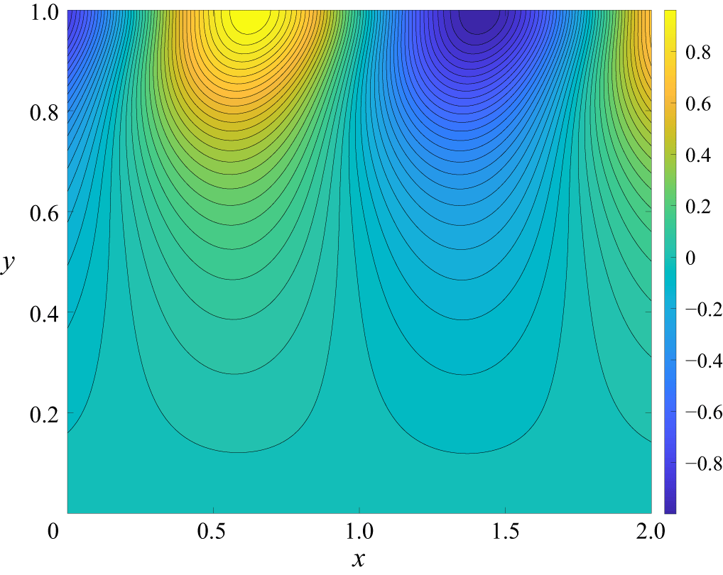
. Contours show the presence of alternating hot and cold spots at the free surface triggered by thermocapillarity. The x-axis length is chosen such that at least two convection cells are captured in the plot. This translates to twice the wavelength of the unstable perturbations.

To understand the physical origin of the instability predicted here, we have obtained contour plots, as shown in figure 4, for the thermal perturbations corresponding to the most unstable mode. For classical thermocapillary instability, convection cells develop as
 $ \textit{Ma}_t$
exceeds
 $ \textit{Ma}_{tc}$
. The thermal perturbations triggered by thermocapillarity lead to alternating cold and hot spots similar to those shown in figure 4. Thus, once thermocapillarity overcomes stabilisation by solutocapillarity, then similar alternating cold and hot spots exist. Based on this, the physical mechanism for the predicted instability could be described as follows.
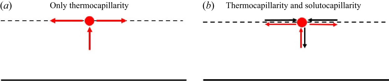
(a) Development of thermocapillary instability at the film–air interface (dotted line). Red arrows indicate the direction of flow due to thermocapillarity and the red dot is the hot spot under consideration. (b) Role of solutocapillary forces in stabilising thermocapillary-induced instability at the air–film interface. Black arrows indicate the direction of flow induced by solutocapillarity.

The physical mechanism behind stabilisation by the lipid layer can be understood as follows. When Marangoni instability arises in a film heated from below, the underlying physical process can be outlined as follows (Smith & Davis Reference Smith and Davis1983; Smith Reference Smith1986; Davis Reference Davis1987; Patne et al. Reference Patne, Agnon and Oron2021a ). The thermal perturbations on the free surface of the liquid layer can generate a localised hot spot, as shown in figure 5(a). Since surface tension decreases with increasing temperature, gradients in temperature cause Marangoni stresses that drive the surface fluid away from this hot spot. To satisfy the mass continuity equation, compensating upward motion emerges from the liquid below towards the surface. Since the fluid beneath is hotter than the surface layer just below the surface (due to heating from below), this upflow delivers additional heat to the surface hot spot. The resulting enhancement in convective heat flux further raises the hot spot temperature, which amplifies thermal perturbations and destabilises the liquid layer.
The impact of solutocapillarity can be incorporated into the above-mentioned mechanism as follows. Thermocapillarity drives the fluid away from the hot spot due to lower surface tension compared with neighbouring points. This flow away from the hot spot reduces surfactant concentration at the hot spot. Since surface tension increases with a decrease in surfactant concentration, an increasing surface tension at the hot spot creates a flow towards the hot spot from neighbouring points. Clearly, the flow created by solutocapillarity is in the opposite direction to the flow created by thermocapillarity, as shown in figure 5(b). This implies that solutocapillarity will weaken the flow away from the hot spot. This, in turn, will weaken the upflow generated in the liquid, which is the supplier of thermal energy to the hot spot necessary for destabilisation, resulting in the stabilisation of the hot spot. This explains the stabilisation of the thermocapillary instability by the lipid layer.
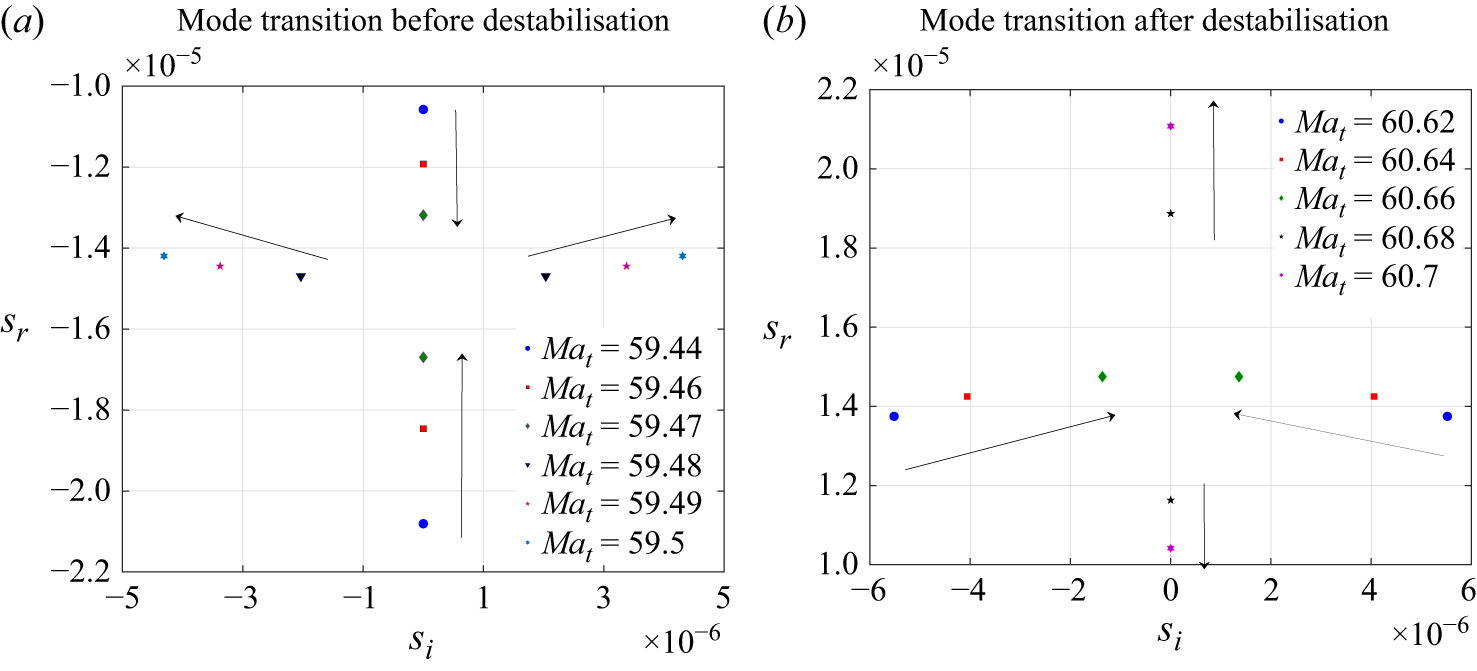
Change in the type of modes (a) from stationary to oscillatory as
 $ \textit{Ma}_t$
approaches
 $ \textit{Ma}_{tc}$
and (b) from oscillatory to stationary as
 $ \textit{Ma}_t$
exceeds
 $ \textit{Ma}_{tc}$
, for
 $ \textit{Ma}_s=30,L_1=0, L_2=0, Ca=0.01, \mu _r=1, A=0$
and
 $k=0.01$
. (a) Mode transition before destabilisation, (b) Mode transition after destabilisation.

As
 $ \textit{Ma}_t \rightarrow Ma_{tc}$
, the film becomes unstable. This stable-to-unstable transition is associated with more complications, as shown in figure 6(a). As indicated by the arrows, just before destabilisation, two least stable stationary modes merge and give rise to two oscillatory modes possessing the same magnitude of
 $s_r$
and
 $s_i$
. These new oscillatory modes travel in opposite directions, implied by the opposite signs of
 $s_i$
. As
 $ \textit{Ma}_t$
is further increased, the oscillatory modes become unstable. Thus, at the onset of instability, the film exhibits oscillatory instability.
From figure 6(a), for
 $ \textit{Ma}_t$
lower than the critical thermal Marangoni number (
 $ \textit{Ma}_{tc}$
), the real part of the growth rate (
 $s_r$
) of the least stable mode decreases with increasing
 $ \textit{Ma}_t$
. In contrast, the second least stable mode
 $s_r$
value increases. The least stable and second least stable modes coalesce at
 $ \textit{Ma}_t \sim Ma_{tc}$
, resulting in two unstable oscillatory modes of the same
 $s_r$
. Figure 3 shows the variation of
 $s_r$
with
 $k$
for the least stable mode, which, as described previously, shows a decrease in
 $s_r$
with
 $ \textit{Ma}_t$
, and hence the observed behaviour.
Further, an increase in
 $ \textit{Ma}_t$
leads to a decrease in
 $s_i$
of the oscillatory modes, but
 $s_r$
keeps on increasing. At a certain value of
 $ \textit{Ma}_t$
, the oscillatory modes merge to give rise to two stationary modes with unequal
 $s_r$
, as shown in figure 6(b). Any further increase in
 $ \textit{Ma}_t$
leads to an increase in
 $s_r$
for one of the newly formed stationary modes and the opposite for the remaining mode. The mode with increasing
 $s_r$
becomes the most unstable mode shown in figure 3.
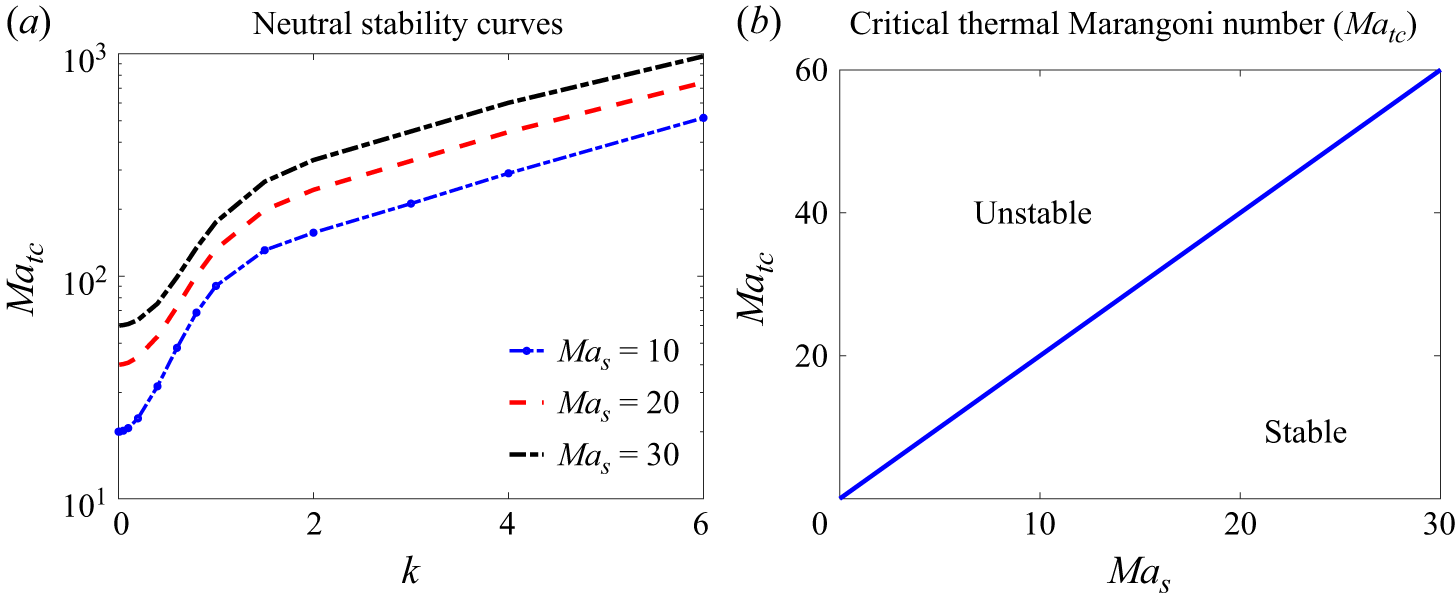
(a) Neutral stability curves and (b) variation of the critical thermocapillary Marangoni number (
 $ \textit{Ma}_{tc}$
) with the solutal Marangoni number for
 $L_1=0, L_2=0, Ca=0.01, \mu _r=1, A=0$
and
 $\delta =0$
. Panel (a) shows that the most unstable mode is longwave. Panel (b) demonstrates the relation
 $ \textit{Ma}_{tc}=2 Ma_s$
.

The preceding discussion shows that the film becomes unstable for
 $ \textit{Ma}_t \gt Ma_{tc}$
for fixed values of
 $ \textit{Ma}_s$
. However, we still do not know the critical wavenumber (
 $k_c$
) necessary to identify the nature of the instability. Thus, the neutral stability curves (corresponding to
 $s_r=0$
) are shown in figure 7(a). The figure demonstrates that the most unstable mode for
 $ \textit{Ma}_t \rightarrow Ma_{tc}$
is longwave since the minima occur at
 $k \rightarrow 0$
, implying
 $k_c=0$
. Using values of
 $ \textit{Ma}_{tc}$
obtained for
 $ \textit{Ma}_s$
values, we plot the variation of
 $ \textit{Ma}_{tc}$
with
 $ \textit{Ma}_s$
in figure 7(b). The presence of a straight line leads to the simple relation
 $ \textit{Ma}_{tc}=2 Ma_s$
. Although not shown here, variation in the capillary number does not affect
 $ \textit{Ma}_{tc}$
values for fixed values of the parameters.
Physically, this implies that a healthy eye would require
 $ \textit{Ma}_t \approx 60$
for destabilisation of the tear film purely due to thermocapillarity. This corresponds to
 $\Delta T = 6\, ^{\circ }\text{C}{-}60 \, ^{\circ }\text{C}$
, depending on the convective heat transfer coefficient value at the film–air interface, which is a function of windspeed. The lower value of
 $\Delta T$
corresponds to a higher windspeed and vice versa. Note that a higher windspeed will lead to a higher temperature gradient across the tear film. Thus, the predictions of the present study are in agreement with clinical observations. For a static wind though,
 $\Delta T = 60 \, ^{\circ }\text{C}$
is necessary for tear-film rupture caused by thermocapillarity. However, as discussed later, in the presence of van der Waals forces,
 $ \textit{Ma}_{tc}=0$
, implying an inherently unstable film. Thus, even for healthy eyes, thermocapillarity could decrease the tear film rupture time.
For diseased eyes suffering from lower secretion of lipids or surfactant due to a malfunctioning meibomian gland (Kim et al. Reference Kim, Ahn, Kim, Kim, Kim and Kim2022),
 $ \textit{Ma}_s$
will be much lower than
 $30$
as discussed at the end of § 4.3. From figure 7(b), this implies a lower value of
 $ \textit{Ma}_t$
is necessary for destabilisation. Thus, a diseased eye is certainly susceptible to thermocapillary-instability-induced destabilisation of the tear film when the ambient air temperature is lower than the cornea temperature.
3.2. Effect of wall slip (
$\delta \neq 0$
)

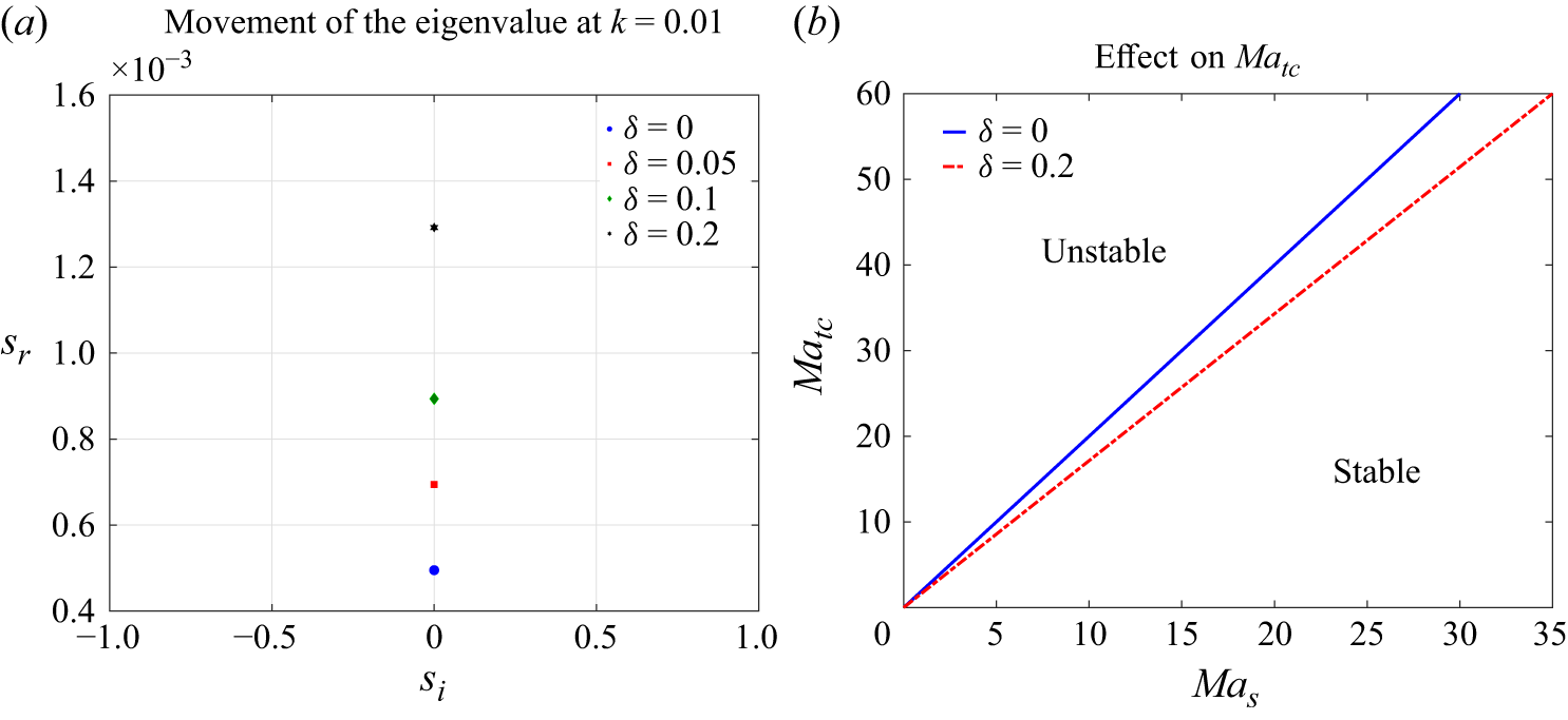
Effect of slip at the film–cornea interface on the stability of tear film. (a) Increasing growth rate of the eigenvalue for increasing slip parameter
 $\delta$
at
 $L_1=0, L_2=0, Ca=0.01, \mu _r=1, A=0$
and
 $ \textit{Ma}_s=30$
, with
 $k=0.01$
. (b) Effect of
 $\delta$
on the critical thermal Marangoni number (
 $ \textit{Ma}_{tc}$
) for a range of solutal Marangoni number (
 $ \textit{Ma}_s$
).

Previous studies by Zhang et al. (Reference Zhang, Craster and Matar2003a
,Reference Zhang, Matar and Craster
b
), Braun (Reference Braun2012) and Dey et al. (Reference Dey, Vivek, Dixit, Richhariya and Feng2020) concluded the destabilising effect of the slip at the film–cornea interface. In the presence of destabilisation caused by thermocapillarity, an increasing slip parameter
 $\delta$
leads to further destabilisation of the tear film shown in figure 8(a). This hints at the lower requirement of the thermal Marangoni number to destabilise the film. Figure 8(b) confirms that this is indeed true since the critical Marangoni number (
 $ \textit{Ma}_{tc}$
) for a film with the slip effect is lower than the corresponding film without slip effect.
The physical mechanism behind destabilisation by the velocity slip could be explained as follows. For a no-slip boundary condition, velocity perturbations vanish at the film–cornea interface. This constrains the base of the tear film, preventing large shear at the substrate and stabilising against disturbances. If slip is allowed (e.g. partial slip due to a glycocalyx layer, irregular surface or weak adhesion), then velocity perturbations in the tear film are not suppressed strongly at the base. This leads to reduced viscous damping, implying less resistance to surface deformations, enhanced shear transmission between air–tear film interface and corneal base, and amplification of Marangoni stresses. Thus, with slip, the perturbation modes (Marangoni waves) penetrate deeper through the film thickness. The cornea no longer acts as a rigid constraint, so disturbances at the air–film interface can resonate through the full thickness. This decreases the influence of the film–cornea interface. Owing to this, for an unstable mode with
 $s_r\gt 0$
, Marangoni stresses remain less affected due to the weakness of constraints at the film–cornea interface, thereby exhibiting a higher
 $s_r$
compared with the no-slip case.
3.3. Effect of elasticity (
$L_1 \neq 0$
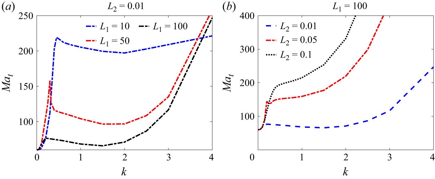
)

Thus far, we have treated the film as a Newtonian liquid film. The tear film also exhibits elasticity due to the presence of mucins in the tear film (Tiffany & Bron Reference Tiffany and Bron1998; Dey et al. Reference Dey, Vivek, Dixit, Richhariya and Feng2020), similar to the pulmonary mucus layer. This particular feature has been neglected in the previous studies. Thus, in this section, we analyse the effect of tear-film viscoelasticity on the stability. The tear-film elasticity leads to two new unstable oscillatory modes as demonstrated in figure 9 provided that the thermal Marangoni number is sufficiently high. Thus, the tear film exhibits oscillatory modes in addition to the Newtonian stationary mode. Henceforth, we will refer to these unstable modes as ‘elastic modes’ to differentiate them from the oscillatory modes discussed previously. Note that the elastic modes become important for
 $k\gt 1$
.
The impact of variation in the tear-film elasticity, i.e.
 $L_1$
, on the tear-film instability is shown in figure 10(a). An increasing elasticity decreases
 $ \textit{Ma}_{tc}$
for the oscillatory modes. The highest value possible for the tear film is
 $L_1=100$
; thus, we have restricted our analysis to
 $L_1 \leqslant 100$
. The impact of an increase in the dimensionless retardation parameter
 $L_2$
is shown in figure 10(b). An increasing
 $L_2$
stabilises the oscillatory modes, thereby increasing
 $ \textit{Ma}_{tc}$
for those modes. This indicates that an increasing contribution of the aqueous part in the total stress leads to stabilisation of the tear film.
Movement of two oscillatory modes arising due to tear film elasticity in
 $s_i-s_r$
plane for
 $L_1=100, L_2=0.01,Ma_s=30,Ca=0.01, \mu _r=1, A=0$
and
 $\delta =0$
.

Neutral stability curves for select values of (a)
 $L_1$
with
 $L_2=0.01$
and (b)
 $L_2$
with
 $L_1=100$
for
 $ \textit{Ma}_s=30,Ca=0.01, \mu _r=1, A=0$
and
 $\delta =0$
. A second minimum for
 $k\gt 1$
, in addition to the low-wavenumber minimum, is due to the presence of elastic oscillatory modes that arise due to tear-film elasticity.

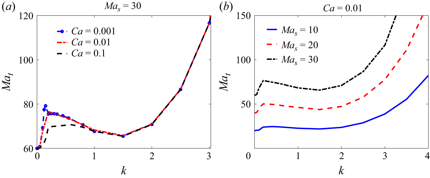
Neutral stability curves for select values of (a)
 $ \textit{Ca}$
with
 $ \textit{Ma}_s=30$
and (b)
 $ \textit{Ma}_s$
with
 $ \textit{Ca}=0.01$
for
 $L_1=100, L_2=0.01,\mu _r=1, A=0$
and
 $\delta =0$
. Figure shows that despite consideration of full range of
 $ \textit{Ca}$
and
 $ \textit{Ma}_s$
possible for a tear film, the longwave instability remains the dominant mode.

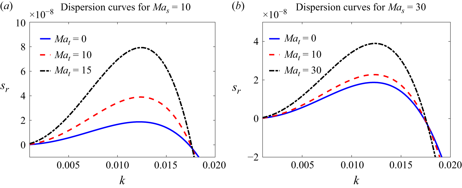
Effect of an increasing thermocapillary Marangoni number (
 $ \textit{Ma}_t$
) on the stability of tear film for two values of solutocapillary Marangoni number (
 $ \textit{Ma}_s$
), viz. dispersion curves for (a)
 $ \textit{Ma}_s=10$
and (b)
 $ \textit{Ma}_s=30$
for
 $L_1=0, L_2=0, Ca=0.01, A=0.001$
and
 $\mu _r=1$
. Both panels demonstrate the destabilisation of the tear film due to an increasing
 $ \textit{Ma}_t$
. Film is unstable even for
 $ \textit{Ma}_t=0$
due to van der Waals forces, implying vanishing critical thermocapillary Marangoni number
 $ \textit{Ma}_{tc}=0$
.

The effect of variation in the capillary number (
 $ \textit{Ca}$
) and solutal Marangoni number (
 $ \textit{Ma}_s$
) is shown in figure 11. From figure 11(b), variation in
 $ \textit{Ca}$
does not affect
 $ \textit{Ma}_{tc}$
for both longwave and elastic instabilities. Thus, the
 $ \textit{Ca}$
value can only affect the growth rate of the perturbation, but does not dictate the onset of instability in the tear film. An increasing
 $ \textit{Ma}_s$
in figure 11(b) shifts the curves to higher
 $ \textit{Ma}_t$
values implying that an increasing solutal Marangoni effect has a stabilising effect on both longwave stationary instability and elastic instability. Additionally, the difference between
 $ \textit{Ma}_{tc}$
for the longwave and elastic modes also increases. Despite that, even for
 $ \textit{Ma}_s=10$
, the difference in
 $ \textit{Ma}_{tc}$
is
 ${\sim} 3$
. This implies that the longwave instability remains the dominant instability mode.
Are these elastic modes the dominant modes of instability for the tear film? The answer is negative, as shown in figure 10. In addition to a minimum at low
 $k$
due to the longwave thermocapillary mode, there is one more minimum for
 $k\gt 1$
due to the elastic modes. A comparison of minima for the longwave and elastic modes shows that even for a maximum value of
 $L_1$
and a minimum value of
 $L_2$
possible for the tear film, the minimum for the oscillatory mode is located well above the longwave mode. To conclude, the elastic modes become unstable at a higher value of
 $ \textit{Ma}_{tc}$
compared with the oscillatory modes for a Newtonian film discussed earlier. Thus, despite tear-film elasticity, the longwave oscillatory modes are the dominant modes of instability, while the elastic modes are sub-dominant. Note that the same conclusion is applicable for any value of
 $ \textit{Ma}_s\lt 30$
.
3.4. Effect of van der Waals forces (
$A\neq 0$
)

By definition, the scaled Hamaker constant is
 $A=A^*/(6 \pi \mu _0 \kappa d)$
with
 $A^* \sim 10^{-19}$
, we obtain
 $A \sim O(10^{-3})$
. For
 $A=0.001$
, the film is unstable even for
 $ \textit{Ma}_t=0$
. Thus, the critical thermocapillary Marangoni number (
 $ \textit{Ma}_{tc}$
) is zero in the presence of van der Waals forces. Thermocapillarity though reinforces the instability caused by van der Waals forces, as shown in figure 12. This indicates that the thermocapillarity induced by the temperature difference between the ambient air and cornea will destabilise the tear film for
 $ \textit{Ma}_t \gt 0$
and not just for
 $ \textit{Ma}_t \gt Ma_{tc}$
. Thus, even for a healthy eye, thermocapillarity induced during winter (due to temperature decrease) will enhance tear-film instability and accelerate tear-film rupture. This could explain why people with otherwise healthy eyes experience dry eye syndrome during winter, as observed in clinical studies by Eidet et al. (Reference Eidet, Aabel, Rasch, Løset, Grønlien, Dartt and Utheim2022).
The physical mechanism behind destabilisation due to van der Waals forces could be explained as follows. The van der Waals interaction energy per unit area is approximately
 $-A^*/(12\pi d^2(1+\xi )^2)$
. This results in a disjoining pressure
 \begin{align} \varPi (h) = -\frac {A^*}{6\pi d^3(1+\xi )^3}. \end{align}
The negative sign indicates that the pressure drives fluid away from thicker regions towards thinner regions, thereby amplifying disturbances at the interface and van der Waals interaction energy could contribute to the perturbation growth. The additional destabilisation due to thermocapillarity shown in figure 12 indicates that van der Waals forces act synergistically. Thus, van der Waals forces support film thinning near the hot spot caused by thermocapillary flow away from the hot spot, resulting in a higher growth rate of perturbations. In nonlinear dynamics, this implies that the film will rupture much earlier due to the thermocapillary effect.
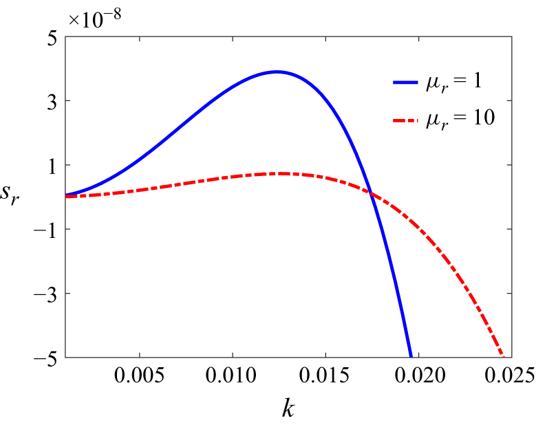
Effect of viscosity variation along the height of tear film on its stability for
 $L_1=0,L_2=0, Ma_s=30,Ca=0.01, A=0.001, Ma_t=10$
and
 $\delta =0$
. The figure demonstrates the stabilisation due to viscosity variation in the tear film.

3.5. Effect of viscosity variation (
$\mu _r \neq 1$
)

Tear film is a multilayered structure with a mucin-dense layer lining the cornea, an aqueous layer deposited on the mucin layer and a lipid layer above the aqueous layer, as shown schematically in figure 1. As discussed in § 2, Prydal et al. (Reference Prydal, Artal, Woon and Campbell1992), Bron et al. (Reference Bron, Tiffany, Gouveia, Yokoi and Voon2004), Braun (Reference Braun2012) and Dey et al. (Reference Dey, Vivek, Dixit, Richhariya and Feng2020) state that mucins are found throughout tear film and form a continuously varying profile. Also, mucin proteins (constituents of the mucus layer) are soluble in water, which does not allow for a sharp interface between mucin and aqueous layers. Based on these observations, Dey et al. (Reference Dey, Vivek, Dixit, Richhariya and Feng2020) proposed a continuous-viscosity model with the highest viscosity at
 $y=0$
and the lowest viscosity at
 $y=1$
(see figure 1). The impact of viscosity variation along film height on tear-film stability is shown in figure 13. Note that
 $\mu _r=1$
corresponds to the absence of viscosity variation. From figure 13, viscosity variation clearly stabilises the tear film in agreement with the predictions of Dey et al. (Reference Dey, Vivek, Dixit, Richhariya and Feng2020). The impact of viscosity variation on tear-film rupture is discussed in § 4.3.
The physical mechanism responsible for the stabilisation due to a decrease in viscosity along the film height could be explained as follows. Referring back to figure 5(a), the flow away from the hot spot leads to an upflow from the inside film. Let us consider a fluid parcel in this upflow. This parcel faces resistance due to fluid viscosity as it moves towards the free surface. For uniform viscosity along the film height, this viscous resistance is constant. However, for a film with a decreasing viscosity with height but with the same average viscosity as a uniform viscosity film, the viscous resistance is maximum in the liquid layer just above the substrate. This implies that the thermocapillary convection has to overcome the bottleneck located near the substrate. This bottleneck then leads to a reduced growth rate of the perturbations shown in figure 13.
4. Longwave model
From § 3, the dominant instability modes are longwave oscillatory modes at the onset of instability, while the elastic modes introduced by the film elasticity are subdominant. Thus, in this section, we will derive the longwave evolution equations using the procedure outlined by Oron et al. (Reference Oron, Davis and Bankoff1997) and Patne et al. (Reference Patne, Agnon and Oron2021b ), and neglect elastic terms in the constitutive equation. Using the derived longwave evolution equations, we will carry out the linear and nonlinear analyses of the system to determine the film rupture.
4.1. Evolution equation derivation
Following Oron et al. (Reference Oron, Davis and Bankoff1997) and Patne et al. (Reference Patne, Agnon and Oron2021b
), we assume the wavelength of the disturbances
 $\varLambda$
is substantially larger than the average thickness of the film
 $d$
, where
 $d=\epsilon \varLambda$
and
 $\epsilon \ll 1$
. To derive the evolution equation, we use the following scaling transformation in the governing equations (2.1):
 $x \to X\epsilon ^{-1}$
,
 $y \to y$
,
 $t \to \tau \epsilon ^{-1}$
,
 $v_x \to U$
,
 $v_y \to \epsilon V$
,
 $T \to T$
,
 $\varGamma \to \varGamma$
and
 $p \to \varPi \epsilon ^{-1}$
. The dimensional local instantaneous film thickness
 $h^*(x^*,t^*)$
is scaled by the mean film thickness
 $d$
. Using these scalings,
 $O(\epsilon ^0)$
governing equations (2.1) are
 \begin{align} - \partial _X \varPi + \partial _y [(\mu _r-(\mu _r-1)y) \partial _y U] =0,\,\, \partial _y \varPi = 0,\,\, \partial ^2_y T=0. \end{align}
Equations (4.1) are subjected to the following boundary conditions. At the film–cornea interface (
 $y=0$
), the assumptions of Navier slip, no-penetration and an imposed temperature imply
 \begin{eqnarray} U=\delta \partial _y U, \quad V=0, \quad T=T_0. \end{eqnarray}
At the film–air interface (
 $y=h(x,t)$
), the tangential and normal stress balance, surfactant concentration advection–diffusion equation and Newton’s cooling law at
 $O(\epsilon ^0)$
respectively yield
 \begin{align} [\mu _r-(\mu _r-1)h] \partial _y U=-\widehat {Ma}_t \partial _X T - \widehat {Ma}_s \partial _X \varGamma , \\[-28pt] \nonumber \end{align}
 \begin{align} \varPi =-\widehat {Ca}^{-1} \partial ^2_X h + \frac {A}{h^3}, \\[-28pt] \nonumber \end{align}
 \begin{align} \partial _y T + BiT = 0, \\[-28pt] \nonumber \end{align}
 \begin{align} \partial _\tau \varGamma + \partial _X (U\!\varGamma ) = 0, \\[-6pt] \nonumber \end{align}
where
 \begin{eqnarray} \widehat {Ma}_t=\epsilon Ma_t, \quad \widehat {Ma}_s=\epsilon Ma_s, \quad \widehat {Ca}=\epsilon ^{-3}Ca, \end{eqnarray}
are the scaled thermal and solutal Marangoni numbers and capillary numbers, respectively. The solution of the
 $O(\epsilon ^0)$
(4.1) yields
 \begin{eqnarray} U = c_2 -\frac {y\partial_X{\kern-1pt}p}{ \mu _r-1} - \frac {\log [\mu _r (y-1) - y] [(\mu _r-1) c_1 + \mu _r \partial _X p]}{(\mu _r-1)^2}, \end{eqnarray}
where
 $c_1$
and
 $c_2$
are integration constants to be determined using the boundary conditions (4.3). The kinematic boundary condition at the film–air interface is
 \begin{eqnarray} \partial _\tau h = -\partial _X \int _0^h U\text{d}y. \end{eqnarray}
Substitution of (4.5) into (4.6) yields longwave evolution equations. For
 $\mu _r \neq 1$
, longwave evolution equations are quite unwieldy. Thus, here, we present longwave evolution equations at
 $\mu _r=1$
. The resulting equations are
 \begin{align} \partial _\tau h & = \partial _X \left [ \left ( \frac {h^3}{3} + \delta h^2 \right ) \partial _X \varPi - \widehat {Ma}_t \frac {(h^2 + \delta h)}{2} \frac {1+Bi}{(1+Bi \, h)^2} \partial _X h \right ] \nonumber \\[4pt]& \quad + \partial _X \left [ \widehat {Ma}_s \frac {(h^2 + \delta h)}{2} \partial _X \varGamma \right ], \end{align}
where the pressure
 $\varPi$
is given by (4.3b
). In (4.7), the first, second and third terms are due to the capillarity, thermocapillarity and soluto-capillarity, respectively. Additionally, the evolution of the surfactant concentration is governed by (4.3d
).
Before proceeding further, we scale back (4.3d ) and (4.7) to yield
 \begin{align} \partial _t h & + \partial _x \left [ \left ( \frac {h^3}{3} + \delta h^2 \right ) \left (Ca^{-1} \partial _x^3 h + 3 A \frac {\partial _X h}{h^4} \right ) + Ma_t \frac {\big(h^2 + \delta h \big)}{2} \frac {1+Bi}{(1+Bi \, h)^2} \partial _x h \right ] \nonumber \\[4pt]& - \partial _x \left [ Ma_s \frac {\big(h^2 + \delta h \big)}{2} \partial _x \varGamma \right ]=0, \\[-28pt] \nonumber \end{align}
 \begin{align} \partial _t \varGamma & + \partial _x \left [\varGamma \left ( \frac {\big(2 \delta h + h^2 \big)}{2} \left (Ca^{-1} \partial _x^3 h + 3 A \frac {\partial _X h}{h^4} \right ) + Ma_t (h + \delta ) \frac {1+Bi}{(1+Bi \, h)^2} \partial _x h \right ) \right ] \nonumber \\[4pt]& - \partial _x \left [Ma_s \varGamma (h + \delta ) \partial _x \varGamma \right ] = 0. \\[0pt] \nonumber \end{align}
The above-coupled equations are the required evolution equations for the tear film. Note that the evolution equation becomes unwieldy to present for
 $\mu _r \neq 1$
; thus, it is not presented here. Due to the scaling used in obtaining the evolution equation, the coefficient of the second term contains
 $1+Bi$
instead of the conventional
 $Bi$
in the same term; see, for instance, (2.63) of Oron et al. (Reference Oron, Davis and Bankoff1997). We will use the above-mentioned equations in the subsequent linear and nonlinear stability analysis.
4.2. Linear stability analysis
To carry out linear stability analysis, substitute
 $h(x,t)=1+h^\prime (x,t)$
and
 $\varGamma (x,t)=1+\varGamma ^\prime (x,t)$
into (4.8) where
 $h^\prime (x,t) \ll 1$
and
 $\varGamma ^\prime (x,t) \ll 1$
are the perturbations imposed on the film height and surfactant concentration, respectively. After substitution, the resulting equations are linearised around the unperturbed height and surfactant concentration. In the linearised equations, we substitute normal modes of the form
 $(h^\prime (x,t),\varGamma ^\prime (x,t)) =(\tilde {h},\tilde {\varGamma })\,\exp (ikx+st )$
where
 $\tilde {h}$
and
 $\tilde {\varGamma }$
are constants. Upon substitution of normal modes, further simplification yields the dispersion relation (for
 $\mu _r=2$
and
 $\delta =0$
)
 \begin{align} & 2 (1 + Bi) Ca s^2 + (1 + Bi) k^4 s ( \log 4 - 1) \nonumber \\ & \quad + Ca k^2 s [-2 Ma_t + (Ma_t + Ma_s + Bi Ma_s) \log 4] \nonumber \\ & \quad - 3 A (1 + Bi) Ca k^2 [s ( \log 4 - 1) + k^2 Ma_s (\log 8-2)] \nonumber \\ & \quad + (1 + Bi) k^6 Ma_s (\log 8-2)=0. \end{align}
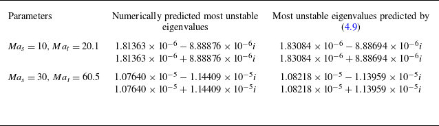
To validate the longwave model, we compare the numerical eigenvalues and those predicted by the above-mentioned dispersion relation in table 2. For
 $k \rightarrow 0$
, the terms with
 $k^4$
and
 $k^6$
can be neglected in (4.9). The solution of the resulting dispersion relation leads to a single root, which will become unstable for
 \begin{eqnarray} Ma_t \gt 2 (1 + Bi) Ma_s \end{eqnarray}
for
 $A=0$
, thus providing an analytical expression for the critical thermal Marangoni number (
 $ \textit{Ma}_{tc}$
). For
 $Bi \ll 1$
, (4.10) yields
 $ \textit{Ma}_{tc}=2 Ma_s$
. This is the exact relation depicted in figure 7(b), thereby providing an analytical proof of a numerically obtained relation. Additionally, from the above-mentioned relation, an increasing wall slip will lead to a decrease in
 $ \textit{Ma}_{tc}$
in agreement with the results shown in figure 8(b).
A comparison of eigenvalues predicted by numerical method outlined in Appendix A and using dispersion relation (4.9). The other parameters are
 $k=0.01, Bi=0.001, Ca=0.01, Pr=100, A=0, \mu _r=1$
and
 $\delta =0$
. The agreement between the eigenvalues shown in the last two columns up to sixth decimal places validates the utility of the derived longwave evolution equation.

4.3. Nonlinear analysis
The preceding discussion on the stability of tear film using the derived longwave evolution equation and in § 3 focus on the linear stability of the film. The surfactant could counteract the influence of thermocapillarity in the nonlinear regime despite the film exhibiting instability. Essentially, does the thermocapillary instability (elaborated in § 3) overcome the influence of the surfactant and lead to tear-film rupture? In this section, we answer this question by performing computations to observe the nonlinear evolution of the perturbations using longwave equation (4.8). These evolution equations have been solved in the domain
 $0\leqslant x\leqslant L$
, using the finite-element-based computational fluid dynamic tool, COMSOL 6.2, where
 $L$
is the length of the computational domain (Lerisson et al. Reference Lerisson, Ledda, Balestra and Gallaire2020; Khanum & Tiwari Reference Khanum and Tiwari2020; Kumawat & Tiwari Reference Kumawat and Tiwari2020). A general form partial differential equation interface and parallel direct sparse solver (PARDISO) were used for computations. The backward differentiation formula is used for numerical time stepping with the initial step size of
 $10^{-3}$
. The time stepping is adaptive. The COMSOL automatically adjusts the time step size during the simulation based on the behaviour of the solution. When the solution evolves slowly, the solver increases the time step to enhance computational efficiency. Conversely, if rapid changes or instabilities occur, it reduces the time step to maintain accuracy and numerical stability.
Beginning with an initially uniform distribution of the surfactant and perturbing the film thickness such that the initial conditions are
 \begin{align} h(x, t=0) = h_0+\zeta \cos \left (\frac {2\pi x}{L}\right ), \\[-28pt] \nonumber \end{align}
 \begin{align} \varGamma (x,t = 0) = \varGamma _0, \\[0pt] \nonumber \end{align}
where
 $\zeta$
is a small number,
 $h_0$
is the base state film thickness and
 $\varGamma _0$
is the initial surfactant concentration, which covers the entire domain uniformly. Following previous works (Zhang et al. Reference Zhang, Craster and Matar2003a
,
Reference Zhang, Matar and Crasterb
), the boundary conditions to carry out the computations are
 \begin{align} \frac {\partial \varGamma }{\partial x} = 0, \quad \frac {\partial h}{\partial x} = \frac {\partial ^3 h}{\partial x^3} = 0, \quad \mathrm{on}\,\, x = 0, \\[-28pt] \nonumber \end{align}
 \begin{align} \frac {\partial \varGamma }{\partial x} = 0, \quad \frac {\partial h}{\partial x} = \frac {\partial ^3 h}{\partial x^3} = 0, \quad \mathrm{on}\,\, x = L. \\[0pt] \nonumber \end{align}
Typical values of the number of elements in the periodic domains are
 $4000$
for a numerically stable solution, while maintaining an optimal computation time and an absolute tolerance of
 $10^{-9}$
is used for the nonlinear computations. The base state
 $h_0 = 1$
is perturbed with the fastest growing linear mode such that the periodic domain is
 $L = L_m = 2\pi /k_m$
. The spatial domain is scaled with respect to periodicity
 $L$
,
 $\chi = x/L$
.
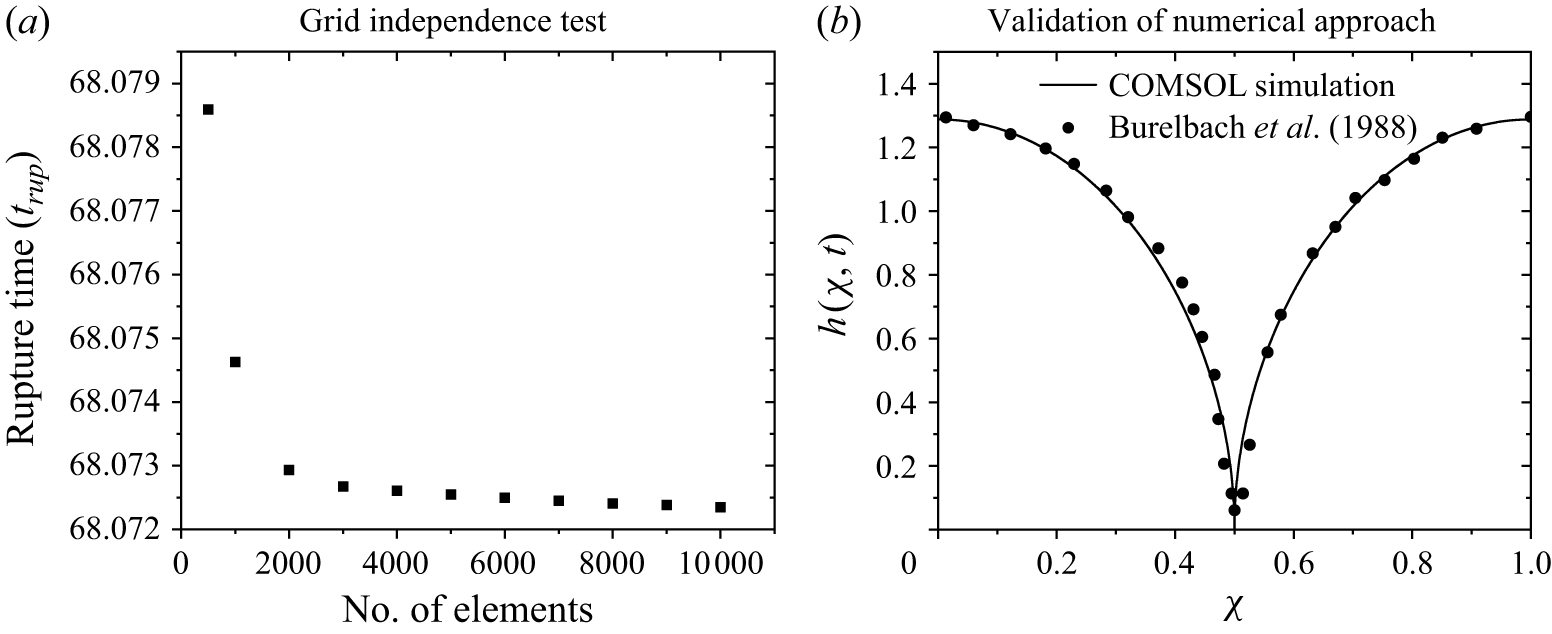
(a) Grid independence test showing the variation of rupture time with the number of mesh elements. (b) Validation of the numerical approach by comparing the tear fluid–air interface profile at the moment of rupture.

Before presenting detailed numerical results, a grid independence test was performed, as shown in figure 14(a), where the rupture time
 $t_{\textit{rup}}$
was evaluated by varying the mesh element size. Based on this analysis, 4000 mesh elements were chosen for the simulations, since further refinement produced negligible changes in rupture time. In addition, we validated our numerical approach in COMSOL by comparing the instantaneous interface profile at the moment of rupture with the results reported by Burelbach, Bankoff & Davis (Reference Burelbach, Bankoff and Davis1988), as shown in figure 14(b). As shown, our results are in good agreement with the numerical scheme of Burelbach et al. (Reference Burelbach, Bankoff and Davis1988), thus confirming the reliability of our simulations.
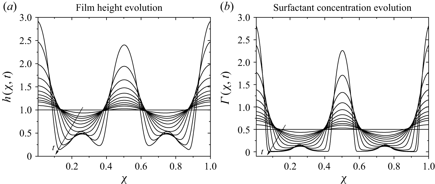
(a) Spatio-temporal film thickness and (b) corresponding surfactant evolution profiles computed at
 $Bi = 0.001$
,
 $ \textit{Ma}_t = 25$
,
 $ \textit{Ca} = 0.01$
,
 $ \textit{Ma}_s$
= 10,
 $A=0$
and
 $\mu _r=1$
. The film ruptures at 49.92 dimensionless time units.

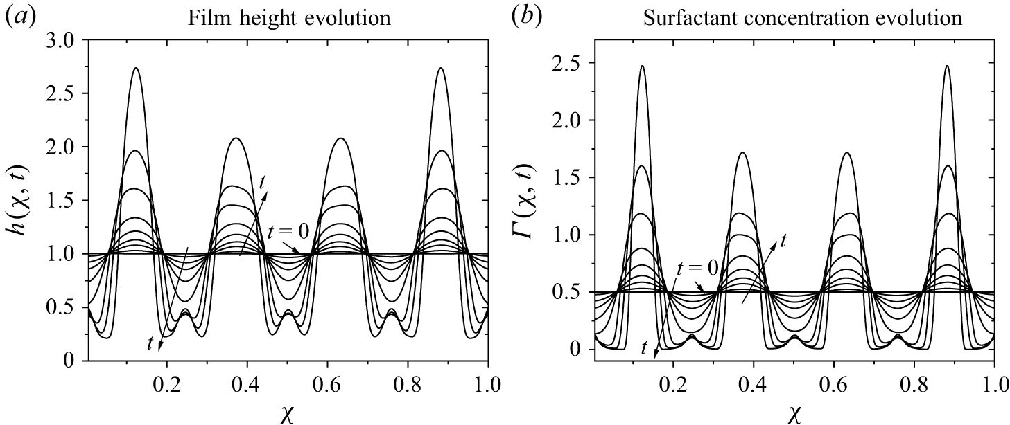
(a) Spatio-temporal film thickness and (b) corresponding surfactant evolution profiles computed at
 $Bi = 0.001$
,
 $ \textit{Ma}_t = 65$
,
 $ \textit{Ca} = 0.01$
,
 $ \textit{Ma}_s = 30$
,
 $A=0$
and
 $\mu _r=1$
. The film ruptures at 20.5 dimensionless time units.

First, we try to investigate the role of pure thermocapillarity in causing film rupture. Figure 15 represents spatio-temporal evolution profiles of film height,
 $h$
, and surfactant concentration (lipid layer),
 $\varGamma$
. As discussed earlier, non-uniform interfacial temperature at the aqueous layer–air interface generates a surface tension gradient, inducing thermocapillary stress that drives liquid from regions of low surface tension (thinner areas) to regions of high surface tension (thicker areas). Similarly, surfactant concentration gradients due to fluid flow generate solutocapillary stresses. In contrast to thermocapillarity, solutocapillary stresses stabilise the thin tear film by driving the liquid from the thicker to the thinner film regions. However, for the parameters considered in figure 15, thermocapillary stresses overcome the stabilising effect of solutocapillary stresses, ultimately leading to film rupture, as shown in figure 15(a). The corresponding surfactant profiles are shown in figure 15(b), where it can be observed that surfactant concentration reduces to nearly zero in the thinner film region, enhancing thermocapillary stress. This destabilises the film and ultimately leads to its rupture.
The film height and surfactant concentration evolution at larger values of
 $ \textit{Ma}_t = 65$
and
 $ \textit{Ma}_s = 30$
are shown in figures 16(a) and 16(b), respectively. At
 $t=20.5$
, the surfactant concentration approaches zero in the thinner film region, allowing thermocapillary stresses to dominate. As a result, the film becomes increasingly thinner and eventually ruptures. The results shown in figures 15 and 16 clearly demonstrate that despite the stabilising effect of the lipid layer, the thermocapillarity succeeds in rupturing the tear film. Thus, the thermocapillarity introduced by the difference between the ambient air and cornea temperatures will lead to film rupture. This occurs for
 $ \textit{Ma}_t\gt 0$
, implying a lower ambient temperature.
The base state is perturbed with the linear mode of
 $k_m$
wavenumber. Thus, in our numerical simulations, we track the fastest-growing linear mode to probe for film rupture. The wavenumber range of perturbations with maximum growth rate for figures 15 and 16 is
 $k_m \sim (0.01{-}0.1)$
. This translates to dimensional wavelength
 $\lambda \sim O(10^{-4}{-}10^{-5})$
m based on the tear-film thickness. This length is clearly compatible with the lateral eye dimensions. In the literature, clinical observations by Eidet et al. (Reference Eidet, Aabel, Rasch, Løset, Grønlien, Dartt and Utheim2022) concluded that during the winter season, the tear film rupture time could be as low as 1 s. However, their analysis does not provide any data from which we could extract the wavelength of the perturbations responsible for the film rupture. Thus, we could not carry out a comparison with the existing clinical observations.
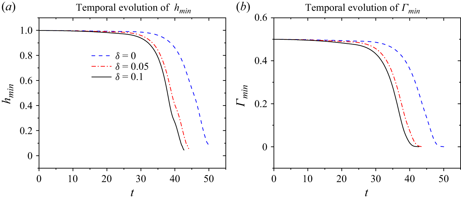
Effect of slip parameter on the temporal evolution of the tear-film and surfactant concentration. The values of other parameters are
 $ \textit{Ma}_t = 25$
,
 $ \textit{Ma}_s = 10$
,
 $ \textit{Ca} = 0.01$
, ,
 $A=0$
,
 $\mu _r=1$
and
 $Bi = 0.001$
. (a) Temporal evolution of
 $h_{\textit{min}}$
, (b) Temporal evolution of
 $\varGamma _{\textit{min}}$
.

The effect of the slip coefficient on the minimum values of film thickness,
 $h$
, and surfactant concentration,
 $\varGamma$
, is reported in figure 17. The rupture time reduces as the value of
 $\delta$
increases, as shown in figure 17(a), whereas the evolution of
 $\varGamma _{\textit{min}}$
is presented in figure 17(b). It is evident from the figure that when surfactant concentration becomes zero, film rupture takes place and the time at which this occurs is termed as rupture time (
 $t_{\textit{rup}}$
).
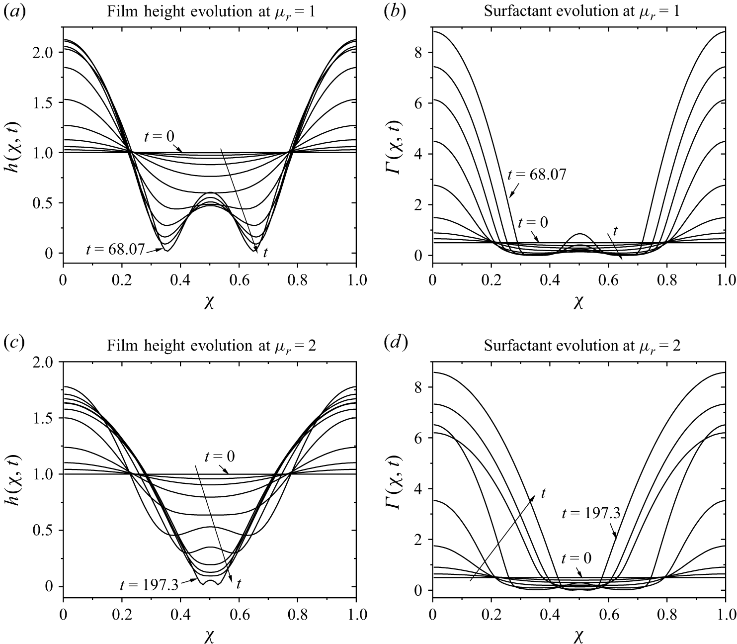
Spatio-temporal film thickness and corresponding surfactant evolution profiles computed at
 $Bi = 0.001$
,
 $ \textit{Ma}_t = 12$
,
 $ \textit{Ca} = 0.01$
,
 $ \textit{Ma}_s$
= 2 and
 $A = 0.001$
. (a) Film height evolution at
 $\mu _r = 1$
,(b) surfactant evolution at
 $\mu _r =1$
,(c) film height evolution at
 $\mu _r = 2$
,(d) surfactant evolution at
 $\mu _r = 2$
.

Previous analyses by Sharma & Ruckenstein (Reference Sharma and Ruckenstein1984, Reference Sharma and Ruckenstein1986), Zhang et al. (Reference Zhang, Craster and Matar2003a ,Reference Zhang, Matar and Craster b ), Braun et al. (Reference Braun, Usha, McFadden, Driscoll, Cook and King-smith2012), Dey et al. (Reference Dey, Vivek, Dixit, Richhariya and Feng2020) and others extensively investigated the role of van der Waals forces in causing tear film rupture. In addition, Dey et al. (Reference Dey, Vivek, Dixit, Richhariya and Feng2020) investigated the effect of continuous viscosity variation on tear-film rupture. Owing to this, we will not present results for tear-film rupture due to van der Waals forces or the effect of a purely viscosity-variation profile. Instead, we will focus on the combined role of van der Waals forces, viscosity variation and thermocapillarity in the subsequent discussion.
Note that consideration of
 $\mu _r \neq 1$
poses a new problem as follows. For
 $\mu _r \neq 1$
, from the velocity profile (4.5), a new logarithmic term
 $\log [\mu _r - (\mu _r -1)y]$
arises in film velocity. This term enters as
 $\log [\mu _r - (\mu _r -1)h]$
in the longwave evolution equations. During numerical solution, if the maximum film height is
 $h_{\textit{max}}\gt \mu _r/(\mu _r-1)$
, then the logarithmic term leads to a singularity and the COMSOL solver cannot proceed with further numerical calculations. Thus, we can numerically solve equations only up to time
 $t$
such that the logarithmic term does not lead to a singularity. This imposes a strong restriction on the choice of parameters for simulation. In our analysis, we found that for
 $\mu _r=2$
, the numerical solution does proceed for a wide range of other parameters. Thus, in the subsequent analysis, we have considered
 $\mu _r=2$
.
The evolution of the film height and surfactant concentration over time, considering non-trivial van der Waals forces, viscosity variation and thermocapillarity, is shown in figure 18, obtained by numerically solving (4.8a
) and (4.8b
) with the initial conditions (4.11) and (4.12). Figures 16(a) and 18(b) correspond to the case where the viscosity ratio
 $\mu _r = 1$
, while figures 18(c) and 18(d) represent the case with
 $\mu _r = 2$
. The viscosity variation along the tear-film height is observed to delay rupture, consistent with the findings of Dey et al. (Reference Dey, Vivek, Dixit, Richhariya and Feng2020). Specifically, the film ruptures at
 $t = 68.07$
when the viscosity is uniform (
 $\mu _r = 1$
), whereas it ruptures later at
 $t = 197.3$
when viscosity varies with film height for
 $\mu _r = 2$
. Thus, rupture time increases by at least one order of magnitude. For
 $\mu _r \in [1,2]$
, we observe a similar trend, indicating that viscosity variation with film height strongly stabilises the tear film. The trend of increasing
 $t_{\textit{rup}}$
with increasing
 $\mu _r$
suggests that for
 $\mu _r\gt 1$
,
 $t_{\textit{rup}} \sim O(10^2 {-} 10^3)$
, depending on other parameters.
The previous discussion concludes that the dimensionless rupture time is
 $O(10^2 {-} 10^3)$
for a tear film, which translates to a dimensional rupture time of
 $O(10^{-1}{-}1)$
s using the scale employed in the present analysis. The predicted rupture time is shorter than the inter-blinking interval of
 $6$
–
 $10$
s. Thus, the tear film can rupture due to the combined effect of thermocapillarity and van der Waals forces. Even in the absence of the thermocapillarity effect, patients suffering from dry eye disease exhibit a tear film rupture time of 2–7 s, with severe cases exhibiting a rupture time of
 ${\sim} 1$
s (Blackie et al. Reference Blackie, Solomon, Scaffidi, Greiner, Lemp and Korb2009; Arita et al. Reference Arita, Itoh, Inoue and Amano2009; Nichols et al. Reference Nichols, Foulks, Bron, Glasgow, Dogru, Tsubota, Lemp and Sullivan2011; Wolffsohn et al. Reference Wolffsohn2017).
Note that meibomian gland dysfunction (MGD) is the leading cause of dry eye syndrome. In MGD patients, lipid layer thickness is often reduced to 20–60 nm, with severe cases showing values
 ${\lt } 20$
nm (McCulley & Shine Reference McCulley and Shine2001). A study using LipiView interferometry reported that MGD patients had a
 $40\,\%{-}60 \,\%$
reduction in lipid layer thickness compared with controls (Arita et al. Reference Arita, Itoh, Inoue and Amano2009). Severe obstructive MGD can reduce lipid secretion to the point that the lipid layer is barely detectable, i.e.
 ${\gt} 70 \,\%$
reduction relative to normal (McCulley & Shine Reference McCulley and Shine2001). If we assume there is a proportional decrease in lipid concentration, then this would imply
 $ \textit{Ma}_s$
for MGD patients to be in the range of 18–12. For severe cases with
 ${\gt} 70 \,\%$
reduction in lipid layer,
 $ \textit{Ma}_s$
could be much lower than
 $9$
. Studies have shown that this leads to dry eye, consistent with clinical observations that MGD patients often exhibit tear film rupture times of 1–3 s, versus
 ${\geqslant} 10$
s in healthy eyes (Blackie et al. Reference Blackie, Solomon, Scaffidi, Greiner, Lemp and Korb2009; Arita et al. Reference Arita, Itoh, Inoue and Amano2009; Nichols et al. Reference Nichols, Foulks, Bron, Glasgow, Dogru, Tsubota, Lemp and Sullivan2011). The inclusion of thermocapillarity is expected to reduce the rupture time below 1 s. Even for healthy eyes, clinical observations by Eidet et al. (Reference Eidet, Aabel, Rasch, Løset, Grønlien, Dartt and Utheim2022) concluded that during the winter season, the tear film rupture time could be as low as 1 s. Furthermore, their clinical observations indicate that compared with the summer season, rupture time during the winter season could be almost halved. In agreement with these studies, our model predicts
 $\sim O(0.1{-}1)$
s, with the lower value applicable to people suffering from dry eye syndrome.
5. Comparison with evaporation-driven tear-film rupture
In the preceding discussion, we focused on the thermocapillary-driven film rupture. However, in the absence of a temperature difference across the tear film, evaporation-driven tear film rupture becomes important. Several studies have investigated this mechanism in detail and provided time and thinning scales associated with the evaporation-driven tear film rupture (Braun Reference Braun2012). Thus, next, we compare the crucial parameters involved in the tear film rupture due to evaporation-driven and thermocapillary-driven instabilities, thereby determining the parametric region where thermocapillary-driven film rupture will become important.
5.1. Comparison of rupture time scales:
Our model predicts that the tear film rupture time is
 $\sim O(0.1{-}1)$
s due to the combined effect of thermocapillarity and van der Waals forces for
 $\Delta T \sim 10\,\text{K}$
. Previous studies (Braun Reference Braun2012; Peng et al. Reference Peng, Cerretani, Braun and Radke2014) suggest the tear film rupture time due to evaporation is
 $\sim O(1{-}10)$
s with lower values for people suffering from the dry eye problem. Note that the rupture time for thermocapillary-driven rupture is strongly temperature-dependent. Thus, under favourable conditions (cold weather), the tear film could follow thermocapillary-driven rupture. To conclude, as the ambient temperature decreases below cornea temperature, thermocapillary-driven tear-film rupture becomes increasingly important, whereas under normal conditions, evaporation-driven tear-film rupture is the preferred pathway.
5.2. Comparison of thinning rates
5.2.1. Evaporative thinning rate
Experimental measurements (Braun Reference Braun2012; Peng et al. Reference Peng, Cerretani, Braun and Radke2014) report evaporative mass fluxes of order
 \begin{align} \dot {m}_e \sim 10^{-7} {-} 10^{-6} \ \mathrm{kg\, m^{-2}\, s^{-1}}. \end{align}
Using the tear density
 $\rho \approx 10^{3}\,\mathrm{kg\,m^{-3}}$
, the corresponding volumetric thinning velocity is
 \begin{align} J_e = \frac {\dot {m}_e}{\rho } \sim 10^{-10} {-} 10^{-9} \ \mathrm{m\, s^{-1}}. \end{align}
This represents a spatially uniform reduction of film thickness.
5.2.2. Thermocapillary-driven thinning rate
Using the tangential stress balance at the air–film interface, the characteristic thermocapillary shear stress is
 \begin{align} \tau _{\textit{TC}} \sim \left | \frac {\partial \sigma }{\partial T} \right | \frac {\Delta T}{\lambda }. \end{align}
Balancing this stress with viscous stress in a film of thickness
 $h$
gives
 \begin{align} \mu \frac {u_{\textit{TC}}}{h} \sim \tau _{\textit{TC}}, \end{align}
and hence,
 \begin{align} u_{\textit{TC}} \sim \frac {h}{\mu } \left | \frac {\partial \sigma }{\partial T} \right | \frac {\Delta T}{\lambda }. \end{align}
The associated volumetric flux per unit width is
 \begin{align} q_{\textit{TC}} \sim u_{\textit{TC}} h = \frac {h^2}{\mu } \left | \frac {\partial \sigma }{\partial T} \right | \frac {\Delta T}{\lambda }. \end{align}
Mass conservation implies a characteristic local thinning rate,
 \begin{align} \left | \partial _t h \right |_{\textit{TC}} \sim \frac {q_{\textit{TC}}}{\lambda } = \frac {h^2}{\mu } \left | \frac {\partial \sigma }{\partial T} \right | \frac {\Delta T}{\lambda ^2}. \end{align}
Using representative physiological values and considering
 $k \sim O(0.01){-}O(0.1)$
, i.e. the perturbations with highest growth rate,
 \begin{align} h &\sim 4 \times 10^{-6}\ \mathrm{m}, \\[-12pt] \nonumber \end{align}
 \begin{align} \mu &\sim 4 \times 10^{-3}\ \mathrm{Pa\,s}, \\[-12pt] \nonumber \end{align}
 \begin{align} \left |\frac {\partial \sigma }{\partial T}\right | &\sim 1.5 \times 10^{-4}\ \mathrm{N\,m^{-1}\,K^{-1}}, \\[-12pt] \nonumber \end{align}
 \begin{align} \Delta T &\sim 10\ \mathrm{K}, \\[-12pt] \nonumber \end{align}
 \begin{align} \lambda &\sim 5 \times 10^{-5}\ \mathrm{m}, \\[10pt] \nonumber \end{align}
we obtain
 \begin{align} \left | \partial _t h \right |_{\textit{TC}} \sim 10^{-3}\ \mathrm{m\,s^{-1}}. \end{align}
5.2.3. Comparison of local thinning
The ratio of thermocapillary-induced local thinning to evaporative thinning is therefore
 \begin{align} \frac { \left | \partial _t h \right |_{\textit{TC}} }{ J_e } \sim 10^{6} {-} 10^{7}. \end{align}
Evaporation produces spatially uniform thinning at a rate
 $O(10^{-10}{-}10^{-9})\,\mathrm{m\,s^{-1}}$
, whereas thermocapillarity can drive lateral mass redistribution and local thickness variations several orders of magnitude faster under realistic temperature gradients and micron-scale wavelengths. As noted for the time scale comparison discussed previously, a substantial temperature difference between the cornea and ambient air is essential for the thermocapillary-driven mechanism to dominate evaporation-driven mechanism. Thus, the predictions obtained in the present study will be applicable only in such parametric regimes.
The previous comparison regarding local thinning must be interpreted with caution due to the following reasons. Evaporation produces a spatially uniform mass loss characterised by a thinning rate
 $J_e$
, whereas thermocapillary stresses generate lateral fluxes that redistribute fluid along the interface. The thinning rate due to thermocapillarity, therefore, represents the local rate of change of film thickness induced by divergence of the lateral flux, rather than a global decay rate. In this sense, the comparison between the two mechanisms should be interpreted as a comparison between uniform thinning and localised thinning due to instability-driven redistribution, rather than as two directly equivalent fluxes. Furthermore, the thermocapillary-driven thinning estimate depends sensitively on the characteristic wavelength of perturbations, scaling as
 $\lambda ^{-2}$
. Thus, the wavelength of the perturbations for the calculation and interpretation of the results must be carefully selected.
6. Summary
The intensification of dry eye symptoms at lower ambient temperatures, particularly during winter, is well known. To understand the underlying fluid mechanics, we have analysed tear-film dynamics in both linear and nonlinear regimes within a thermocapillary framework. The tear film is modelled as a viscoelastic thin film with an insoluble surfactant at the air–film interface, incorporating variation of viscosity along the film height, van der Waals forces and Navier slip at the substrate. In contrast to previous studies, the present model simultaneously accounts for these effects, thereby providing a more comprehensive description of tear-film dynamics.
The general linear stability analysis (GLSA), performed using a pseudospectral method, shows that in the absence of a temperature gradient the tear film remains stable due to strong surfactant-induced stabilisation. When a temperature gradient is introduced, thermocapillary stresses drive instability. In the absence of surfactant effects, this manifests as a stationary longwave instability for positive thermal Marangoni numbers (
 $ \textit{Ma}_t$
). In the presence of surfactant (non-zero
 $ \textit{Ma}_s$
), a competition arises between solutocapillary stabilisation and thermocapillary destabilisation, with instability occurring for
 $ \textit{Ma}_t \gt 2Ma_s$
. At onset, two oscillatory modes become unstable and the neutral stability curves exhibit minima at low wavenumber, confirming the longwave nature of the dominant instability. The physical mechanism underlying this behaviour arises from thermocapillary-driven flow from warmer to cooler regions, which redistributes fluid and amplifies thickness perturbations in competition with surfactant-induced stabilisation.
Inclusion of viscoelastic effects further modifies the stability characteristics. Elasticity extends the oscillatory instability to higher wavenumbers (
 $k\gt 1$
), introducing a secondary minimum in the neutral stability curves. However, for physiologically relevant parameters, this elastic mode requires significantly higher
 $ \textit{Ma}_t$
and the longwave oscillatory mode remains dominant. Navier slip enhances instability by allowing disturbances at the interface to penetrate the full film thickness. The inclusion of van der Waals forces removes the requirement of a critical
 $ \textit{Ma}_t$
for instability and thermocapillarity further amplifies this effect. Physically, thermocapillary flow induces local thinning in warmer regions, which is reinforced by van der Waals attraction, leading to accelerated growth of perturbations. Variation of viscosity along the film height provides partial stabilisation but does not suppress instability.
Since the dominant instability is longwave, we derived reduced longwave evolution equations for film thickness and surfactant concentration. Linear stability analysis of these equations agrees well with the full numerical results. Nonlinear simulations show that thermocapillarity, in combination with van der Waals forces, can lead to rupture within the inter-blinking time. The rupture time depends strongly on
 $ \textit{Ma}_t$
, van der Waals forces and
 $ \textit{Ma}_s$
, and weakly on slip. The required
 $ \textit{Ma}_t$
values and corresponding perturbation wavelengths lie within physiologically realistic ranges, and the predicted rupture times are consistent with clinically observed time scales.
From a practical and clinical perspective, the present study provides a mechanistic explanation for the increased susceptibility to dry-eye symptoms under cold environmental conditions. The analysis shows that reduced ambient temperature enhances thermocapillary stresses, which promote lateral redistribution of the tear film and accelerate local thinning. This effect is particularly pronounced when the lipid layer is weakened, as occurs in meibomian gland dysfunction. The model therefore identifies a coupled thermocapillary–lipid mechanism that links environmental exposure and tear-film instability, and provides quantitative insight into how temperature, lipid properties and intermolecular forces jointly influence rupture. These findings offer a framework for interpreting clinical observations and suggest that controlling thermal gradients and improving lipid-layer properties may help mitigate instability.
While the present model captures key physical mechanisms, several extensions are required for a more complete description. In particular, evaporation and spatial heterogeneities of the ocular surface have been neglected and may influence both the mean thinning rate and rupture dynamics. Future work should incorporate evaporation in a coupled framework to quantify its interaction with thermocapillary-driven redistribution. In addition, extending the model to two spatial dimensions, including realistic ocular surface topography and non-uniform lipid distributions, would enable direct comparison with interferometric imaging of tear-film breakup patterns. Such developments would help bridge the gap between mechanistic modelling and predictive, clinically relevant descriptions of tear-film instability.
Acknowledgements
R.P. acknowledges financial support from the SERB-DST under grant SRG/2023/000223. T.C.K. acknowledges financial support from the Indian Institute of Technology Jodhpur, India, under grant I/SEED/TCK/20230138.
Declaration of interests
The authors report no conflict of interest.
Appendix A. Numerical methodology
To implement the pseudo-spectral method, the eigenfunctions are expanded in the form of a series of Chebyshev polynomials
 \begin{eqnarray} \widetilde {g}(y)=\sum _{j=0}^{j=N} a_{\kern-1pt j} T_{\kern-1pt j} (y), \end{eqnarray}
where
 $N$
is the highest degree of the polynomial in the series expansion or number of collocation points,
 $T_j(y)$
are Chebyshev polynomials of degree
 $j$
, and
 $a_j$
are the unknown series coefficients. Further, the fluid domain is transformed from
 $ 0 \leqslant y \leqslant 1$
to
 $ -1 \leqslant y \leqslant 1$
by using mapping
 $y \rightarrow 2y-1$
. Upon discretisation, using the (A1) yields
 \begin{eqnarray} \boldsymbol{Pe} + s \boldsymbol{Q}\boldsymbol{e}=0, \end{eqnarray}
where
 $\boldsymbol{P}$
and
 $\boldsymbol{Q}$
are matrices derived following the discretisation procedure and
 $\boldsymbol{e}$
is the vector containing the coefficients of all series expansions. The details of the procedure can be found from Trefethen (Reference Trefethen2000), Schmid & Henningson (Reference Schmid and Henningson2001), Patne et al. (Reference Patne, Agnon and Oron2020a
).
To solve the eigenvalue problem (A2), we use the eig MATLAB routine. To remove the numerical spurious eigenvalues, the code is executed for
 $N$
and
 $N+2$
collocation points, and the individual eigenvalues are compared with a specified tolerance, e.g.
 $10^{-5}$
. To further ascertain the genuine eigenvalues, the number of collocation points is increased by
 $25$
and the variation of the eigenvalues is observed. If the eigenvalue does not change more than a specified precision, e.g. to the sixth significant digit, the same number of collocation points is used to determine the eigenspectrum. In the present work,
 $N=50$
is found to be sufficient to achieve convergence and to determine the leading, most unstable eigenvalue within the investigated parameter range. The above-described pseudo-spectral method has been used for similar problems by Patne et al. (Reference Patne, Agnon and Oron2020a
,
Reference Patne, Agnon and Oronb
, Reference Patne, Agnon and Oron2021a
,Reference Patne, Agnon and Oron
b
) and Patne & Oron (Reference Patne and Oron2022). The numerical method employed here is validated against the predictions of the longwave model described in § 4.
Appendix B. Dimensional parameters
In this appendix, we estimate the range of dimensionless parameters relevant to the tear film as follows. The viscosity, density and thickness of the tear film (including mucin layer) are
 ${\sim} 10^{-3}$
Pa s,
 $10^3$
kg m
 $^{-3}$
and
 $4{-}8 \, {\unicode{x03BC}}$
m, respectively (Holly Reference Holly1973; Lin & Brenner Reference Lin and Brenner1982; Tiffany Reference Tiffany1991; Prydal et al. Reference Prydal, Artal, Woon and Campbell1992; Danjo, Nakamura & Hamano Reference Danjo, Nakamura and Hamano1994; Lai et al. Reference Lai, Wang, Wirtz and Hanes2009). The rheological relaxation time for the tear film is
 ${\sim} 10^{-4} ~\text{to}~10^{-3}$
s (Vega, Fernandez & Cardil Reference Vega, Fernandez and Cardil2023). The air–aqueous interface tension is
 $0.072$
Nm−1 at
 $298$
K and the surface diffusivity of the surfactant is
 $\sim 10^{-9}$
m
 $^2$
s−1 (Sharma & Ruckenstein Reference Sharma and Ruckenstein1986). Since
 $\alpha ^*_T$
and
 $\kappa$
are not available for the tear film, we consider the parameters for the water, viz.
 $\alpha ^*_T \sim O(0.1)$
N (mK)−1 and
 $\kappa \sim 10^{-7}$
m
 $^2$
s−1 (Vargaftik, Volkov & Voljak Reference Vargaftik, Volkov and Voljak1983).
To estimate
 $\alpha _\varGamma ^* = {\text{d}\sigma ^*}/{\text{d}\varGamma ^*}$
, we use the values of the air–water interface tension for a clean interface and when the interface is saturated with the surfactant. For a clean air–water interface,
 $\sigma ^*=0.072$
Nm−1 and for surfactant saturated interface from Zhang et al. (Reference Zhang, Matar and Craster2003b
),
 $\sigma ^*=0.044$
Nm−1. This leads to
 $\alpha _\varGamma ^* = {0.028}/{\varGamma ^*_0}$
. Substituting this in the definition of
 $ \textit{Ma}_s$
makes sure that the
 $\varGamma ^*_0$
value is unnecessary. The thermal conductivity of tear film and heat convection coefficient at the air–water interface are
 $k_{th} =0.6$
W (m K)−1 and
 $q \sim 10{-}10^3$
W (m
 $^2$
K)−1, respectively. The thermal conductivity and molecular diffusivity in the surfactant lipid layer are
 $\kappa _s \sim 10^{-8}$
W (m K)−1 and
 $D_m \sim 10^{-11}$
m
 $^2$
s−1 (Ebersberger et al. Reference Ebersberger, Schindler, Kirsch, Pluhackova, Schambony, Seydel, Böckmann and Unruh2020). These dimensional parameters are used in estimating dimensionless parameters in table 1.