1 Introduction
A shear layer is a region across which the fluid velocity changes appreciably. In many situations of interest, the shear layer thickness is typically thin relative to other length scales in the problem. In the limit of zero thickness one arrives at the high Reynolds number model of a shear layer known as a vortex sheet. The vorticity in the shear layer is then confined to the mathematical surface describing the sheet and thus becomes a singular distribution. Kinematically, this is represented by a jump in the tangential velocity across the sheet. The problem becomes an inviscid one that is governed by the Euler equations and with the sheet being a material surface. Since the sheet vorticity is infinite, the quantity known as the sheet strength density is defined as the integral of vorticity in the direction normal to the sheet.
For the case of a two-dimensional free vortex sheet in an otherwise quiescent surrounding, the self-induced dynamics is governed by the Birkhoff–Rott equation. With
 $\unicode[STIX]{x1D6FE}(s,t)$
as the strength density, the problem can be transformed by letting
 $\unicode[STIX]{x1D6E4}(s,t)$
be a Lagrangian parameter describing the amount of circulation in the sheet as measured from a reference point with coordinate
 $s$
. Then
 $\unicode[STIX]{x1D6FE}(s,t)=\unicode[STIX]{x2202}\unicode[STIX]{x1D6E4}/\unicode[STIX]{x2202}s$
and for a point
 $z=s\text{e}^{\text{i}\unicode[STIX]{x1D703}(s)}$
on the sheet the complex conjugate velocity
 $\unicode[STIX]{x2202}\overline{z}/\unicode[STIX]{x2202}t=u-\text{i}v$
of the sheet is:
 $$\begin{eqnarray}u-\text{i}v=\frac{1}{2\unicode[STIX]{x03C0}\text{i}}\int \frac{\unicode[STIX]{x1D6FE}(s^{\prime })\,\text{d}s^{\prime }}{z(s)-z(s^{\prime })}=\frac{1}{2\unicode[STIX]{x03C0}\text{i}}\int \frac{\text{d}\unicode[STIX]{x1D6E4}^{\prime }}{z(\unicode[STIX]{x1D6E4})-z(\unicode[STIX]{x1D6E4}^{\prime })},\end{eqnarray}$$
where the Cauchy principal value is implied and the integration is over the entirety of the sheet; explicit dependence on
 $t$
, time, has been omitted for notational clarity. This equation is dynamical as it ensures continuity of pressure everywhere across the sheet (Saffman Reference Saffman1992) including a shedding edge if present. While seemingly innocuous, this nonlinear singular equation presents considerable mathematical difficulties to those seeking its solution. The successful similarity solution of Kaden (Reference Kaden1931) for a semi-infinite vortex sheet gave the rolled-up spiral structure of the inner core. For the finite vortex sheet, Kaden’s solution is assumed to be applicable to the two sheet tips at very small times.
To circumvent the difficulties, many other investigations of roll-up have discretized the sheet into elements that make the evolution dynamics more tractable. Rosenhead (Reference Rosenhead1931) famously was the first to use a point vortex discretization and investigated the evolution of a periodic perturbation to the sheet. Westwater (Reference Westwater1935) used the same point vortex method to study the roll-up of the finite vortex sheet left behind an elliptically loaded wing. For nearly half a century the apparent success of these two studies remained somewhat mysterious. Perhaps now infamously, their results were difficult, if not impossible, to recreate with improved numerical capability (e.g. Moore Reference Moore1971). Instead, chaotic motion of the point vortices occurred when the spatial and temporal resolutions were refined (also see Saffman & Baker Reference Saffman and Baker1979).
Moore (Reference Moore1974) stated that the main reason the chaotic motion ensues is an inability of the point vortices to satisfactorily represent the inner spiral. As such, while retaining the point vortex discretization, he introduced a tip vortex representing the overall effect of the spiral core, an idea attributed to Smith (Reference Smith1968). As vortices approach the core they are amalgamated into the tip vortex with a user-defined criterion, which is also referred to as ‘core dumping’. Chorin & Bernard (Reference Chorin and Bernard1973) used the cutoff or vortex blob method to regularize the singular point vortices and exhibited smooth roll-up, at least initially. Krasny & coworkers have systematically studied and significantly improved upon this method (Krasny Reference Krasny1986a , Reference Krasny1987; Nitsche & Krasny Reference Nitsche and Krasny1994; Krasny & Nitsche Reference Krasny and Nitsche2002).
Fink & Soh (Reference Fink and Soh1978) convincingly argue that the issue is a more fundamental one associated with the point vortex method. They showed that this discretization inherently neglects logarithmic contributions to the Cauchy principal value integral. They proposed a rediscretization of the vortices that causes the logarithmic terms to vanish. Baker (Reference Baker1980) gave a more thorough error analysis of their method and showed that another source of error appears as a result of neglecting the effect of sheet curvature, which becomes significant and unavoidable in the spiral.
After these foundational papers (there are several others we have not mentioned here), the 1980s marked major improvements in the calculation of vortex sheet roll-up via vortex panel methods (Hoeijmakers & Vaatstra Reference Hoeijmakers and Vaatstra1983; Sugioka & Widnall Reference Sugioka and Widnall1985). These methods use a combination of numerical techniques to obtain a smooth roll-up including a rediscretization process, core dumping and patching the numerical solution of the inner spiral with that of Kaden’s similarity solution as given by Pullin (Reference Pullin1978). Higdon & Pozrikidis (Reference Higdon and Pozrikidis1985) used a higher-order interpolation method for the sheet shape and strength distribution along with a point-insertion procedure to capture the initial roll-up of a Kelvin–Helmholtz instability. The vortex blob method (for a comparison of different regularization kernels see Baker & Pham Reference Baker and Pham2006) has brought continued success to the study of vortex dynamics including complex unsteady three-dimensional motions (e.g. Lindsay & Krasny Reference Lindsay and Krasny2001).
Point vortex methods cannot explicitly account for the effect of sheet curvature, but judicious choices of the spacing and number of vortices can yield an accurate representation of the sheet evolution. Also, special numerical techniques can be employed to produce more stable calculations, such as point insertion combined with a shock-capturing scheme to resolve steep gradients (Sohn, Yoon & Hwang Reference Sohn, Yoon and Hwang2010). However, the concept of the Cauchy principal value integral defining the induced velocity at a single point on the sheet requires infinite resolution. An attempt to estimate the local contribution by direct computation of the limit results in near-singular values of opposing sign that must appropriately cancel, which can be problematic and arbitrary. As such, for any discretization of the sheet into finite elements, e.g. segments, the self-induced velocity of that element must also be considered and is yet another effect neglected by point vortex methods. Conventional vortex panel methods provide an unrealistic model of the self-induced velocity giving logarithmically divergent velocities at the edges of the panel and thus, in a sense, reclaim the issue of the principal value limit.
Pozrikidis (Reference Pozrikidis2000) discusses the evaluation of the principal value singularity without a regularizing kernel. Two main methods were investigated and he demonstrated the success of each up to a certain time when the calculations succumb to numerical instabilities, which can be increased by employing various regularization, smoothing and/or adaptive rediscretization techniques. The first is an indirect method based on the generalized vortex methods of Baker (Reference Baker1983) in which a decomposition of the velocity field contains a vector potential representing the flow induced by the vortex sheet. Derivatives of this potential are computed to obtain the velocity the sheet induces on itself. The second method is a direct one in which the singularity of the Birkhoff–Rott equation (or more generally the Biot–Savart equation) is subtracted off and its contribution is accounted for through the use of integral identities. Pozrikidis states that this method relaxes the constraint on the geometrical smoothness of the sheet (i.e. a continuously varying normal vector) that is interrupted by typical discretizations of the sheet into approximated elements. While these methods reduce the order of the singularity, the results still contain weak singularities, which we opt to avoid in the current study.
In this paper, we revisit the inviscid roll-up problem with the aim of providing a realistic model of the self-induced velocity of a sheet segment while also maintaining the integrity of the sheet as a continuous object, thus capturing the effect of curvature. The true dynamics of the sheet must include both of these features. The model is based on the physical principle of a bounded velocity and allows direct integration through the singularity as opposed to circumventing the singularity, such as in the methods discussed by Pozrikidis (Reference Pozrikidis2000). In the next section we briefly review the method of Fink & Soh (Reference Fink and Soh1978), which is then followed by the details of our proposed model and we show how it essentially includes their method as a special case. The numerics of the method are described in § 3. Example calculations of a finite vortex sheet with the elliptical circulation distribution are presented in § 4. The Kelvin–Helmholtz instability of a periodically disturbed infinite vortex sheet is investigated in § 5. Throughout, the term ‘panel’ implies a planar element, whereas ‘segment’ refers to an element with arbitrary curvature.
2 Mathematical formulation
Fink & Soh (Reference Fink and Soh1978) showed the appearance of logarithmic and higher-order terms that are neglected by a point vortex method. The vortex sheet is divided into
 $N$
straight line panels whose motion is determined from that of pivotal points
 $z_{j}$
. The sheet strength on each panel is represented by the Taylor series
 $\unicode[STIX]{x1D6FE}_{k}(\unicode[STIX]{x1D70E})=\sum _{p=0}\unicode[STIX]{x1D6FE}_{k}^{(p)}\unicode[STIX]{x1D70E}^{p}/p!$
, where
 $\unicode[STIX]{x1D70E}$
is a local coordinate measured from the pivotal point,
 $\unicode[STIX]{x1D6FE}_{k}^{(p)}$
is the
 $p$
th derivative of
 $\unicode[STIX]{x1D6FE}_{k}$
at
 $\unicode[STIX]{x1D70E}=0$
. The
 $k=j$
panel induces a velocity on itself,
 $\unicode[STIX]{x0394}(u-\text{i}v)_{j,j}$
, that must be included in (1.1). Then including the induced velocities
 $\unicode[STIX]{x0394}(u-\text{i}v)_{j,k}$
from all other
 $k\neq j$
panels gives, to first-order approximation, the total velocity of the
 $j$
th point
 $(u-\text{i}v)_{j}$
as:
 $$\begin{eqnarray}(u-\text{i}v)_{j}\approx \underbrace{\frac{1}{2\unicode[STIX]{x03C0}\text{i}}\mathop{\sum }_{k\neq j}\frac{\unicode[STIX]{x1D6E4}_{k}}{z_{j}-z_{k}}}_{\text{sheet}\;\text{remainder}}-\underbrace{\frac{\text{e}^{-\text{i}\unicode[STIX]{x1D703}_{j}}}{2\unicode[STIX]{x03C0}\text{i}}\left[\unicode[STIX]{x1D6FE}_{j}^{(0)}\log \left(\frac{\unicode[STIX]{x0394}s_{j}^{+}}{\unicode[STIX]{x0394}s_{j}^{-}}\right)+\unicode[STIX]{x1D6FE}_{j}^{(1)}(\unicode[STIX]{x0394}s_{j}^{+}+\unicode[STIX]{x0394}s_{j}^{-})\right]}_{j\text{-}\text{th}\;\text{panel}\;\text{self}\text{-}\text{induced}\;\text{velocity}},\end{eqnarray}$$
where
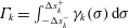 $\unicode[STIX]{x1D6E4}_{k}=\int _{-\unicode[STIX]{x0394}s_{k}^{-}}^{\unicode[STIX]{x0394}s_{k}^{+}}\unicode[STIX]{x1D6FE}_{k}(\unicode[STIX]{x1D70E})\,\text{d}\unicode[STIX]{x1D70E}$
is the circulation in the
 $k$
th panel,
 $\unicode[STIX]{x0394}s_{j}^{\pm }$
are the lengths of the partial panels from
 $\unicode[STIX]{x1D70E}=0$
to the two endpoints and
 $\unicode[STIX]{x1D703}_{j}$
is the angle of inclination of the
 $j$
th panel. Clearly the summation term represents a point vortex system approximating the sheet remainder, but also present are the aforementioned logarithmic and higher-order terms. The rediscretization places the pivotal points at the midpoints of the panels so that
 $\unicode[STIX]{x0394}s_{j}^{+}=\unicode[STIX]{x0394}s_{j}^{-}\equiv \unicode[STIX]{x0394}s_{j}/2$
and the
 $\log$
term vanishes. The remaining term is the first in the series
 $\sum _{p=1}\unicode[STIX]{x1D6FE}_{j}^{(p)}(\unicode[STIX]{x0394}s_{j})^{p}/(p\cdot p!)[1-(-1)^{p}]$
so that the even terms are zero, leaving just the odd terms and in using (2.1) they state that the error is
 $O(\unicode[STIX]{x0394}s_{j}^{3})$
. However, Baker (Reference Baker1980) showed that the error is actually
 $O(\unicode[STIX]{x0394}s_{j})$
due to effect of curvature having been neglected.
2.1 The self-induced velocity: single segment
Next, we derive a model for the self-induced velocity of the
 $j$
th segment that yields a closed-form result in a single term rather than an infinite series. Consider a point
 $s^{\prime }$
on a sheet segment of length
 $2\unicode[STIX]{x0394}s$
where the local coordinate is
 $s$
and let
 $\unicode[STIX]{x1D6FF}\unicode[STIX]{x1D6E4}$
be the small amount of circulation (change) near
 $s^{\prime }$
. This infinitesimal circulation induces a velocity whose local functionality is
 $\unicode[STIX]{x1D6FF}u\sim (\unicode[STIX]{x1D6FF}\unicode[STIX]{x1D6E4}/[s-s^{\prime }])\approx \unicode[STIX]{x1D6FE}(\unicode[STIX]{x1D6FF}s/[s-s^{\prime }])$
, where the definition
 $\unicode[STIX]{x1D6FE}=\unicode[STIX]{x2202}\unicode[STIX]{x1D6E4}/\unicode[STIX]{x2202}s$
was invoked. For this
 $\unicode[STIX]{x1D6FF}u$
to remain finite it is required that
 $\unicode[STIX]{x1D6FE}\sim [s-s^{\prime }]/\unicode[STIX]{x1D6FF}s$
. Then, if we parameterize this segment as
 $s=-\unicode[STIX]{x0394}s\cos \unicode[STIX]{x1D719}$
with
 $0\leqslant \unicode[STIX]{x1D719}\leqslant \unicode[STIX]{x03C0}$
we obtain:
 $$\begin{eqnarray}\tilde{\unicode[STIX]{x1D6FE}}(\unicode[STIX]{x1D719};\unicode[STIX]{x1D719}^{\prime })\sim \frac{\cos \unicode[STIX]{x1D719}^{\prime }-\cos \unicode[STIX]{x1D719}}{\sin \unicode[STIX]{x1D719}},\end{eqnarray}$$
where
 $\unicode[STIX]{x1D719}^{\prime }$
corresponds to the parameterization of the point of interest
 $s^{\prime }=-\unicode[STIX]{x0394}s\cos \unicode[STIX]{x1D719}^{\prime }$
, that is where the self-induced velocity is evaluated. Note that while the coordinate
 $s$
is measured relative to the midpoint of the segment we have not yet considered any specific point on the segment at which to evaluate the induced velocity. To show the physical significance of this term, the integration is first performed over a small sub-range encompassing the primed point:
 $(\unicode[STIX]{x1D719}^{\prime }-\unicode[STIX]{x0394}\unicode[STIX]{x1D719}_{-})\rightarrow (\unicode[STIX]{x1D719}^{\prime }+\unicode[STIX]{x0394}\unicode[STIX]{x1D719}_{+})$
which is of length
 $\unicode[STIX]{x0394}\unicode[STIX]{x1D719}=\unicode[STIX]{x0394}\unicode[STIX]{x1D719}_{+}+\unicode[STIX]{x0394}\unicode[STIX]{x1D719}_{-}$
. Assuming the segment to be straight with inclination angle
 $\unicode[STIX]{x1D703}$
, the local induction of just this sub-segment is:
 $$\begin{eqnarray}\displaystyle \unicode[STIX]{x0394}(u-\text{i}v) & = & \displaystyle -\frac{\text{e}^{-\text{i}\unicode[STIX]{x1D703}}}{2\unicode[STIX]{x03C0}\text{i}}\int _{\unicode[STIX]{x1D719}^{\prime }-\unicode[STIX]{x0394}\unicode[STIX]{x1D719}_{-}}^{\unicode[STIX]{x1D719}^{\prime }+\unicode[STIX]{x0394}\unicode[STIX]{x1D719}_{+}}\left[\frac{\tilde{\unicode[STIX]{x1D6FE}}(\unicode[STIX]{x1D6FC};\unicode[STIX]{x1D719}^{\prime })}{\cos \unicode[STIX]{x1D719}-\cos \unicode[STIX]{x1D6FC}}\right]\sin \unicode[STIX]{x1D6FC}\,\text{d}\unicode[STIX]{x1D6FC}\nonumber\\ \displaystyle & = & \displaystyle -\frac{\text{e}^{-\text{i}\unicode[STIX]{x1D703}}}{2\unicode[STIX]{x03C0}\text{i}}\left[\unicode[STIX]{x1D6FC}+\tilde{\unicode[STIX]{x1D6FE}}(\unicode[STIX]{x1D719};\unicode[STIX]{x1D719}^{\prime })\log \left|\frac{1+\tilde{\unicode[STIX]{x1D6FE}}(\unicode[STIX]{x1D719};\unicode[STIX]{x03C0})\tan (\unicode[STIX]{x1D6FC}/2)}{1-\tilde{\unicode[STIX]{x1D6FE}}(\unicode[STIX]{x1D719};\unicode[STIX]{x03C0})\tan (\unicode[STIX]{x1D6FC}/2)}\right|\right]_{\unicode[STIX]{x1D6FC}=\unicode[STIX]{x1D719}^{\prime }-\unicode[STIX]{x0394}\unicode[STIX]{x1D719}_{-}}^{\unicode[STIX]{x1D719}^{\prime }+\unicode[STIX]{x0394}\unicode[STIX]{x1D719}_{+}},\end{eqnarray}$$
where the integration is with respect to the dummy variable
 $\unicode[STIX]{x1D6FC}$
and we see a similar logarithmic term. However, we note that this logarithmic term is distinctly different from that obtained by Fink & Soh (Reference Fink and Soh1978). This is because they expanded the vortex sheet strength in a Taylor series prior to integration so that their log term corresponds to the leading term in that expansion. We can further reveal the connection with their method by letting the point of interest, that is
 $\unicode[STIX]{x1D719}^{\prime }$
, correspond to the midpoint of the segment. Then the limit
 $\unicode[STIX]{x0394}\unicode[STIX]{x1D719}\rightarrow 0$
on the above equation yields:
 $$\begin{eqnarray}\unicode[STIX]{x0394}(u-\text{i}v)\approx -\frac{\text{e}^{-\text{i}\unicode[STIX]{x1D703}}}{2\unicode[STIX]{x03C0}\text{i}}\left[\unicode[STIX]{x0394}\unicode[STIX]{x1D719}+\underbrace{(-\unicode[STIX]{x0394}\unicode[STIX]{x1D719}+O(\unicode[STIX]{x0394}\unicode[STIX]{x1D719}^{3})+\cdots +O(\unicode[STIX]{x0394}\unicode[STIX]{x1D719}^{2n-1}))}_{\text{logarithmic}\;\text{term}}\right],\end{eqnarray}$$
where
 $n$
is any positive integer thus showing that the
 $\log$
term is expressed as a series of odd powers in
 $\unicode[STIX]{x0394}\unicode[STIX]{x1D719}$
(when
 $\unicode[STIX]{x1D719}^{\prime }$
is not the midpoint even terms appear). This is the same feature as the series that led to the first-order term in (2.1). The connection with the method of Fink & Soh (Reference Fink and Soh1978) is apparent.
Now, upon returning to (2.3) we see that by setting
 $\unicode[STIX]{x1D719}=\unicode[STIX]{x1D719}^{\prime }$
the logarithmic term vanishes identically since
 $\tilde{\unicode[STIX]{x1D6FE}}(\unicode[STIX]{x1D719}^{\prime };\unicode[STIX]{x1D719}^{\prime })=0$
. More importantly, this is the case for
 $\unicode[STIX]{x1D719}^{\prime }$
representing any point along the segment, not specifically the midpoint. The self-induced velocity on the sub-segment is simply
 $\unicode[STIX]{x0394}(u-\text{i}v)=-(\text{e}^{-\text{i}\unicode[STIX]{x1D703}}/2\unicode[STIX]{x03C0}\text{i})\unicode[STIX]{x0394}\unicode[STIX]{x1D719}$
, but having assumed a planar segment the error is
 $O(\unicode[STIX]{x0394}s)$
as mentioned above. We also note that there are no higher-order terms that remain because we have represented the self-induced velocity with a closed-form expression containing a single term. The meaning of this is that the potentially singular log term of Fink & Soh (Reference Fink and Soh1978) would be balanced by their infinite series of remainder terms. In other words, when the physics of the problem is considered at the level of the sheet strength, the intuitive result is a finite velocity that does not depend on the choice of how the sheet is discretized.
The above procedure can be followed on every sub-segment
 $\unicode[STIX]{x0394}\unicode[STIX]{x1D719}$
that makes up the original segment. Then (2.3) can be integrated over the whole segment from
 $0\rightarrow \unicode[STIX]{x03C0}$
and by putting
 $\tilde{\unicode[STIX]{x1D6FE}}(\unicode[STIX]{x1D6FC};\unicode[STIX]{x1D719}^{\prime }=\unicode[STIX]{x1D719})$
the self-induced velocity on the segment is:
 $$\begin{eqnarray}\unicode[STIX]{x0394}(u-\text{i}v)=\frac{\text{i}}{2}\text{e}^{-\text{i}\unicode[STIX]{x1D703}}=\frac{1}{2}(\sin \unicode[STIX]{x1D703}+\text{i}\cos \unicode[STIX]{x1D703})\quad \forall \unicode[STIX]{x1D719}\in [0,\unicode[STIX]{x03C0}]\end{eqnarray}$$
so that a uniform velocity is induced normal to the segment over the whole of itself. This equation will be recognized as the self-induced velocity of a planar vortex sheet with an elliptical circulation distribution (put
 $\unicode[STIX]{x1D719}^{\prime }=\unicode[STIX]{x03C0}/2$
in (2.2)). This is in contrast to vortex panel methods (e.g. Sugioka & Widnall Reference Sugioka and Widnall1985) where the logarithmically divergent velocity is due to the assumption of a constant strength density along the panel. In fact, this is the same logarithmic term found by Fink & Soh (Reference Fink and Soh1978) because the leading term in their expansion of
 $\unicode[STIX]{x1D6FE}(s)$
corresponds to a zero-order approximation of a constant strength density; see the first term in square brackets in (2.1).
Instead, equation (2.2) represents the limiting form that
 $\unicode[STIX]{x1D6FE}(s)$
will take for the local contribution of the
 $j$
th segment to the Cauchy principal value of the Birkhoff–Rott equation. Since
 $\tilde{\unicode[STIX]{x1D6FE}}(\unicode[STIX]{x1D719}^{\prime };\unicode[STIX]{x1D719}^{\prime })=0$
, then this form can be added to
 $\unicode[STIX]{x1D6FE}(s)$
without effecting the actual strength density or circulation distributions. For dimensional consistency
 $\tilde{\unicode[STIX]{x1D6FE}}$
is multiplied by some constant
 $q_{j}$
. However, this
 $q_{j}$
is not given by a local approximation of
 $\unicode[STIX]{x1D6FE}(s)$
, such as
 $\unicode[STIX]{x0394}\unicode[STIX]{x1D6E4}/\unicode[STIX]{x0394}s$
. The reason can be seen by considering that when
 $\unicode[STIX]{x0394}s_{j}\rightarrow 0$
then
 $\unicode[STIX]{x1D719}^{\prime }\rightarrow \unicode[STIX]{x1D719}$
and so
 $\tilde{\unicode[STIX]{x1D6FE}}(\unicode[STIX]{x1D719};\unicode[STIX]{x1D719}^{\prime })\rightarrow 0$
, as it should since this then leaves only the ‘true’
 $\unicode[STIX]{x1D6FE}(s)$
at the point
 $s$
(see (2.7) below). The determination of the
 $q_{j}$
is discussed in § 2.4.
2.2 Segmented vortex sheet
The previous subsection showed that the segment discretization of the vortex sheet can be defined arbitrarily. Moreover, the approximation of a planar segment is only required for the local contribution to the Cauchy principal value integral, that is the self-induced velocity. For numerical purposes, it is convenient to also consider the sheet as a ‘mesh’ of
 $N+1$
points. While we maintain these points to be the end points of the
 $N$
segments, the self-induced velocity expression applies to any straight segment regardless of whether it is defined by its endpoints, midpoint or any other point(s). Next, we parameterize the sheet and each of the
 $j=1\ldots N$
segments of respective arclengths
 $2s_{o}$
and
 $2\unicode[STIX]{x0394}s_{j}$
as:
 $$\begin{eqnarray}s=-s_{o}\cos \unicode[STIX]{x1D719}\quad s_{j}=-\unicode[STIX]{x0394}s_{j}\cos \unicode[STIX]{x1D719}_{j}\quad s_{o}=\mathop{\sum }_{j=1}^{N}\unicode[STIX]{x0394}s_{j},\end{eqnarray}$$
where
 $0\leqslant \unicode[STIX]{x1D719},\unicode[STIX]{x1D719}_{j}\leqslant \unicode[STIX]{x03C0}$
. Then, recalling that the self-induced velocity term does not add circulation, the expression for the sheet strength density may be written:
 $$\begin{eqnarray}\unicode[STIX]{x1D6FE}(s)=\unicode[STIX]{x1D6FE}(\unicode[STIX]{x1D719})+q_{j}\frac{\cos \unicode[STIX]{x1D719}_{j}^{\prime }-\cos \unicode[STIX]{x1D719}_{j}}{\sin \unicode[STIX]{x1D719}_{j}}.\end{eqnarray}$$
The total velocity induced along the
 $j$
th segment by the whole of the sheet is:
 $$\begin{eqnarray}(u-\text{i}v)_{j}=\frac{\text{i}q_{j}}{2}\text{e}^{-\text{i}\unicode[STIX]{x1D703}_{j}}+\frac{1}{2\unicode[STIX]{x03C0}\text{i}}\left[\int _{0}^{\unicode[STIX]{x1D719}_{l}^{j}}\frac{\unicode[STIX]{x1D6FE}(\unicode[STIX]{x1D719}^{\prime })s_{o}\sin \unicode[STIX]{x1D719}^{\prime }\,\text{d}\unicode[STIX]{x1D719}^{\prime }}{z_{j}-z(\unicode[STIX]{x1D719}^{\prime })}+\int _{\unicode[STIX]{x1D719}_{r}^{j}}^{\unicode[STIX]{x03C0}}\frac{\unicode[STIX]{x1D6FE}(\unicode[STIX]{x1D719}^{\prime })s_{o}\sin \unicode[STIX]{x1D719}^{\prime }\,\text{d}\unicode[STIX]{x1D719}^{\prime }}{z_{j}-z(\unicode[STIX]{x1D719}^{\prime })}\right],\end{eqnarray}$$
where the first term is the self-induced velocity,
 $\unicode[STIX]{x1D719}_{l}^{j}$
and
 $\unicode[STIX]{x1D719}_{r}^{j}$
are the values of
 $\unicode[STIX]{x1D719}$
at the left and right endpoints of the
 $j$
th segment and
 $z_{j}=z(\unicode[STIX]{x1D719})$
for
 $\unicode[STIX]{x1D719}\in [\unicode[STIX]{x1D719}_{l}^{j},\unicode[STIX]{x1D719}_{r}^{j}]$
. The integrals in (2.8) may be written as the sum
 $Q_{j,k}\equiv \sum _{k\neq j}\unicode[STIX]{x0394}(u-\text{i}v)_{j,k}$
where:
 $$\begin{eqnarray}\unicode[STIX]{x0394}(u-\text{i}v)_{j,k}=\frac{1}{2\unicode[STIX]{x03C0}\text{i}}\int _{0}^{\unicode[STIX]{x03C0}}\frac{\unicode[STIX]{x1D6FE}(\unicode[STIX]{x1D719}_{k})\unicode[STIX]{x0394}s_{k}\sin \unicode[STIX]{x1D719}_{k}\,\text{d}\unicode[STIX]{x1D719}_{k}}{(z_{j,o}-z_{k,o})-(\unicode[STIX]{x0394}s_{j}\cos \unicode[STIX]{x1D719}_{j})\text{e}^{\text{i}\unicode[STIX]{x1D703}_{j}(\unicode[STIX]{x1D719}_{j})}+(\unicode[STIX]{x0394}s_{k}\cos \unicode[STIX]{x1D719}_{k})\text{e}^{\text{i}\unicode[STIX]{x1D703}_{k}(\unicode[STIX]{x1D719}_{k})}}\end{eqnarray}$$
and is the velocity contribution induced by the
 $k$
th segment on the
 $j$
th with
 $z_{j,o}$
and
 $z_{k,o}$
as the complex locations of the midpoints of these segments. The possibility of
 $\unicode[STIX]{x1D6FE}(\unicode[STIX]{x1D719}_{k})$
,
 $\unicode[STIX]{x1D703}_{k}(\unicode[STIX]{x1D719}_{k})$
and
 $\unicode[STIX]{x1D703}_{j}(\unicode[STIX]{x1D719}_{j})$
varying along their respective segments is not precluded. The forms in (2.8) and (2.9) reiterate that the assumption of a planar segment is only required for the self-induced velocity and the effects of sheet curvature can be captured insofar as the sheet shape is well-represented by spline interpolation (Baker Reference Baker1980).
2.3 Neighbouring segments
Consider the neighbouring
 $k=j\pm 1$
segments that are on the right and left of the
 $j$
th one. If
 $\unicode[STIX]{x0394}s$
is appropriately small then we can assume that
 $\unicode[STIX]{x0394}s_{k}\approx \unicode[STIX]{x0394}s_{j}$
,
 $\unicode[STIX]{x1D703}_{k}\approx \unicode[STIX]{x1D703}_{j}$
, and
 $(z_{j,o}-z_{j\pm 1,o})\approx \mp 2\unicode[STIX]{x0394}s_{j}\text{e}^{\text{i}\unicode[STIX]{x1D703}_{j}}$
. Similarly, assuming that the strength density does not vary much over these segments,
 $\unicode[STIX]{x1D6FE}(\unicode[STIX]{x1D719}_{k})\approx \unicode[STIX]{x1D6FE}_{o}$
, then the induced velocity becomes approximately:
 $$\begin{eqnarray}\frac{\unicode[STIX]{x1D6FE}_{o}\text{e}^{-\text{i}\unicode[STIX]{x1D703}_{j}}}{2\unicode[STIX]{x03C0}\text{i}}\left[\underbrace{\log \left|\frac{1-\cos \unicode[STIX]{x1D719}_{j}}{3-\cos \unicode[STIX]{x1D719}_{j}}\right|}_{j-1\;\text{segment}}+\underbrace{\log \left|\frac{3+\cos \unicode[STIX]{x1D719}_{j}}{1+\cos \unicode[STIX]{x1D719}_{j}}\right|}_{j+1\;\text{segment}}\right].\end{eqnarray}$$
The neighbouring segments induce infinite velocities at the endpoints of the
 $j$
th segment, that is at
 $\unicode[STIX]{x1D719}_{j}=0$
and
 $\unicode[STIX]{x03C0}$
. However, as
 $\unicode[STIX]{x0394}s_{j}\rightarrow 0$
then the segment shrinks to the single point at its centre, namely
 $\unicode[STIX]{x1D719}_{j}=\unicode[STIX]{x03C0}/2$
, so that the
 $\log$
terms cancel and the velocity remains finite. Hence, the discretization fabricates this issue and it is actually correct to omit the singular contributions on the endpoints. Moreover, as
 $\unicode[STIX]{x0394}s_{j}\rightarrow \unicode[STIX]{x1D716}>0$
the result should be the local contribution to the Cauchy principal value integral, which we have already accounted for with the self-induced velocity
 $(\text{i}q_{j}/2)\text{e}^{-\text{i}\unicode[STIX]{x1D703}_{j}}$
.
The self-induction of two adjacent sheet segments from some time
 $t=t_{n}$
to
 $t_{n}+\unicode[STIX]{x0394}t$
. The
 $q_{j}$
and
 $\unicode[STIX]{x1D703}_{j}^{\prime }$
are determined by requiring the induced velocities at the mutual endpoint are equal; see (2.12).

2.4 Stretching the sheet with
 $q_{j}$

The unknown constants
 $q_{j}$
are related to the magnitude of the self-induced velocity. A given endpoint belongs to two different segments and is thus subjected to two different self-induced velocities, which recall are normal to the segment. The vorticity equation is
 $\text{D}\unicode[STIX]{x1D714}/\text{D}t=\unicode[STIX]{x2202}\unicode[STIX]{x1D714}/\unicode[STIX]{x2202}t+\boldsymbol{u}\boldsymbol{\cdot }\unicode[STIX]{x1D735}\unicode[STIX]{x1D714}=0$
and letting
 $\unicode[STIX]{x1D6FE}(s)=\unicode[STIX]{x1D6FF}(n)\unicode[STIX]{x1D714}(s)$
with
 $n$
being the sheet normal coordinate, then we may write:
 $$\begin{eqnarray}\int \left[\frac{\unicode[STIX]{x2202}\unicode[STIX]{x1D714}}{\unicode[STIX]{x2202}t}+\boldsymbol{u}\boldsymbol{\cdot }\unicode[STIX]{x1D735}\unicode[STIX]{x1D714}\right]\text{d}n\approx \frac{\unicode[STIX]{x2202}\unicode[STIX]{x1D6FE}}{\unicode[STIX]{x2202}t}+u_{s}\frac{\unicode[STIX]{x2202}\unicode[STIX]{x1D6FE}}{\unicode[STIX]{x2202}s}=0.\end{eqnarray}$$
Now considering the two adjacent segments shown in figure 1, we see that the self-induced velocity of each segment stretches its neighbour and will elongate the sheet. This is a feature not accounted for in point vortex methods, nor vortex panel methods where
 $\unicode[STIX]{x1D6FE}$
is assumed constant on each panel. Hence, the self-induced velocity physically represents the transport of vorticity by advective stretching of the sheet and is most important at locations on the sheet where the tangential sheet velocity and/or the gradient of the strength density along the sheet are large. The presence of these features are usually the locations where roll-up occurs. For example, the tip of a finite vortex sheet typically has an infinite strength density, which is often cited as the reason for the initial roll-up (Pullin & Phillips Reference Pullin and Phillips1981), and the Kelvin–Helmholtz instability resulting from a sinusoidal perturbation to an infinite vortex sheet of initially constant strength density shows roll-up beginning at the locations where the perturbation has concentrated vorticity such that
 $\unicode[STIX]{x2202}\unicode[STIX]{x1D6FE}/\unicode[STIX]{x2202}s$
is largest.
Now, in reality the sheet deforms continuously in time and space. With the representation of the sheet as a segmented object, we can consider that the inclination angle of the segment between time steps, say
 $\unicode[STIX]{x1D703}_{j}^{\prime }$
, is also unknown. Moreover, the self-induction should not be discontinuous, which yields the following equations:
 $$\begin{eqnarray}\left[\frac{\text{i}q_{j}}{2}\text{e}^{-\text{i}\unicode[STIX]{x1D703}_{j}^{\prime }}+Q_{j,k}\right]_{\unicode[STIX]{x1D719}_{j}=0}=\left[\frac{\text{i}q_{j-1}}{2}\text{e}^{-\text{i}\unicode[STIX]{x1D703}_{j-1}^{\prime }}+Q_{j-1,k}\right]_{\unicode[STIX]{x1D719}_{j-1}=\unicode[STIX]{x03C0}},\end{eqnarray}$$
where again
 $Q_{j,k}=\sum _{k\neq j}\unicode[STIX]{x0394}(u-\text{i}v)_{j,k}$
is the velocity induced on the
 $j$
segment due to the
 $k\neq j$
segments. These equations ensure that the left endpoint of the
 $j$
segment moves with the same self-induced velocity as the right endpoint of the
 $(j-1)$
segment and are used to determine
 $q_{j}$
and
 $\unicode[STIX]{x1D703}_{j}^{\prime }$
. The difference between the
 $Q_{j,k}$
terms is how the neighbouring segments are treated (recall § 2.3) when a given point on the sheet is considered to belong to the
 $j$
or
 $(j-1)$
segment; this is discussed further in § 3.2. This bypasses the difficulty of a discontinuous normal vector (Pozrikidis Reference Pozrikidis2000).
3 Numerical method
In this section the rediscretization procedure and calculation of the self-induced velocity for a general sheet are discussed. Additional numerical treatments required for specific problems are discussed in beginning of §§ 4 and 5 where the cases of finite and infinite vortex sheets are investigated.
3.1 Rediscretization
Let the vortex sheet be comprised of
 $j=1\ldots N$
segments or
 $n=1\ldots (N+1)$
mesh points. For the rediscretization we essentially use the interpolation scheme described by Baker (Reference Baker1980). Namely, a chord length parameter defines the members of the set
 $\{\unicode[STIX]{x1D706}_{n}\}$
as:
 $$\begin{eqnarray}\unicode[STIX]{x1D706}_{n}=\mathop{\sum }_{k=1}^{n-1}|z_{k+1}-z_{k}|,\end{eqnarray}$$
and is used in a spline interpolation to approximate
 $z(\unicode[STIX]{x1D706})$
. The derivative of the interpolated function
 $|\text{d}z/\text{d}\unicode[STIX]{x1D706}|$
is evaluated at a chosen number of
 $M$
locations
 $\{\unicode[STIX]{x1D706}_{m}\}$
and these are integrated to give the arclength at points
 $\{s_{m}\}$
; Baker recommends that
 $M\geqslant 2(N+1)$
. Then a new set of arclength points
 $\{s_{p}\}$
are prescribed with a desired spacing to interpolate the points
 $\{\unicode[STIX]{x1D706}_{p}\}=\unicode[STIX]{x1D706}(\{s_{p}\})$
. Finally, the set of rediscretized points
 $\{z_{p}\}$
are interpolated from
 $\{z_{n}\}$
,
 $\{\unicode[STIX]{x1D706}_{n}\}$
and
 $\{\unicode[STIX]{x1D706}_{p}\}$
, and may contain more or less points than the original
 $(N+1)$
.
Any other variable corresponding to the rediscretized points may be found by interpolating with
 $\{\unicode[STIX]{x1D706}_{n}\}$
and
 $\{\unicode[STIX]{x1D706}_{p}\}$
. If desired we may also rediscretize to points corresponding to equal intervals of the sheet parameter
 $\unicode[STIX]{x1D719}$
. We term the spacing options as
 $s$
-spacing and
 $\unicode[STIX]{x1D719}$
-spacing. Alternatively, once the equal-arclength rediscretization has been performed, then the points may be re-interpolated to correspond to equal spacing of other quantities, such as the circulation.
3.2 Calculation procedure
When the sheet strength is infinite there is also an infinite induced velocity. However, it is impossible to preserve this feature numerically if
 $\unicode[STIX]{x1D6FE}$
is used in the calculations. Therefore, we opt to describe the sheet with the differential change in circulation
 $\text{d}\unicode[STIX]{x1D6E4}$
, which remains finite and preserves circulation. As a result we revert to the left-hand side of (1.1), and (2.8) is easily converted to this formulation since
 $\unicode[STIX]{x1D6FE}(\unicode[STIX]{x1D719})s_{o}\sin \unicode[STIX]{x1D719}\,\text{d}\unicode[STIX]{x1D719}=\unicode[STIX]{x1D6FE}(s)\,\text{d}s=\text{d}\unicode[STIX]{x1D6E4}$
. The sheet integration is then from
 $\unicode[STIX]{x1D6E4}=0$
to
 $\unicode[STIX]{x1D6E4}_{s}$
, with
 $\unicode[STIX]{x1D6E4}_{s}$
being the total circulation.
Assigning the
 $p$
-interpolation described above to produce the same number of original points
 $p=n=1\ldots (N+1)$
, then with the circulation interpolated to the same spacing we may write:
 $$\begin{eqnarray}z_{n}=z(\unicode[STIX]{x1D706}(s_{n})),\quad \unicode[STIX]{x1D6E4}_{n}=\unicode[STIX]{x1D6E4}(\unicode[STIX]{x1D706}(s_{n}))\quad \rightarrow \quad z_{n}=z(\unicode[STIX]{x1D6E4}_{n}).\end{eqnarray}$$
The
 $n$
th mesh point on the sheet belongs to the
 $j$
and
 $(j-1)$
segments, so that the velocity induced at the
 $n$
th point is:
 $$\begin{eqnarray}\displaystyle & \displaystyle (u-\text{i}v)_{n}=\frac{\text{i}q_{j}}{2}\text{e}^{-\text{i}\unicode[STIX]{x1D703}_{j}^{\prime }}+\frac{\text{i}q_{j-1}}{2}\text{e}^{-\text{i}\unicode[STIX]{x1D703}_{j-1}^{\prime }}+Q_{n} & \displaystyle\end{eqnarray}$$
 $$\begin{eqnarray}\displaystyle & \displaystyle Q_{n}=\frac{1}{2\unicode[STIX]{x03C0}\text{i}}\left[\int _{0}^{\unicode[STIX]{x1D6E4}_{n-1}}\frac{\text{d}\unicode[STIX]{x1D6E4}_{k}}{z_{n}-z_{k}}+\int _{\unicode[STIX]{x1D6E4}_{n+1}}^{\unicode[STIX]{x1D6E4}_{s}}\frac{\text{d}\unicode[STIX]{x1D6E4}_{k}}{z_{n}-z_{k}}\right]. & \displaystyle\end{eqnarray}$$
For a sheet divided into
 $j=1\ldots N$
segments,
 $q_{j}$
and
 $\unicode[STIX]{x1D703}_{j}^{\prime }$
are
 $2N$
unknowns to be determined from (2.12) which represents
 $2(N-1)$
real equations. The system is closed by a given boundary condition (e.g. symmetry, stagnation point) at the end(s) of the sheet so that
 $q_{1}$
and
 $\unicode[STIX]{x1D703}_{1}^{\prime }$
are either known or inferred. In the latter case, the equations are solved iteratively until
 $|\boldsymbol{X}_{m}-\boldsymbol{X}_{m-1}|<\unicode[STIX]{x1D716}$
at the
 $m$
iteration where
 $\boldsymbol{X}=(q_{1},\ldots ,q_{N},\unicode[STIX]{x1D703}_{1}^{\prime },\ldots ,\unicode[STIX]{x1D703}_{N}^{\prime })$
and
 $\unicode[STIX]{x1D716}$
is a chosen threshold.
With the given boundary condition then (2.12) is used to determine
 $q_{j}$
and
 $\unicode[STIX]{x1D703}_{j}^{\prime }$
for the
 $2\leqslant j\leqslant N$
segments:
 $$\begin{eqnarray}\displaystyle \frac{\text{i}q_{j}}{2}\text{e}^{-\text{i}\unicode[STIX]{x1D703}_{j}^{\prime }}=\frac{\text{i}q_{j-1}}{2}\text{e}^{-\text{i}\unicode[STIX]{x1D703}_{j-1}^{\prime }}+(Q_{j-1,k}-Q_{j,k}). & & \displaystyle\end{eqnarray}$$
The above
 $Q_{j,k}$
terms are calculated by integrals similar to that for
 $Q_{n}$
, but by omitting the contribution from the neighbouring segments (recall § 2.3). Since the difference of these terms is required, then we may reduce the calculation to:
 $$\begin{eqnarray}\displaystyle (Q_{j-1,k}-Q_{j,k})=\frac{1}{2\unicode[STIX]{x03C0}\text{i}}\left[\int _{\unicode[STIX]{x1D6E4}_{n-2}}^{\unicode[STIX]{x1D6E4}_{n-1}}\frac{\text{d}\unicode[STIX]{x1D6E4}_{k}}{z_{n}-z_{k}}-\int _{\unicode[STIX]{x1D6E4}_{n+1}}^{\unicode[STIX]{x1D6E4}_{n+2}}\frac{\text{d}\unicode[STIX]{x1D6E4}_{k}}{z_{n}-z_{k}}\right]. & & \displaystyle\end{eqnarray}$$
Since the functions are interpolated, then the integration may be performed as desired. For the ease of implementation, we use the trapezoid rule on the
 $n$
mesh points. Ideally, a fourth-order Runge–Kutta time-integration scheme will be used, but a different time-integration scheme may be used when the sheet strength is infinite.
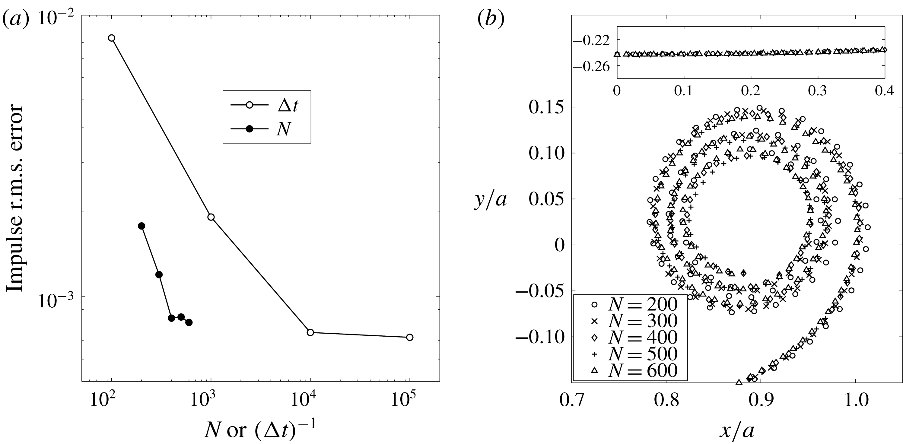
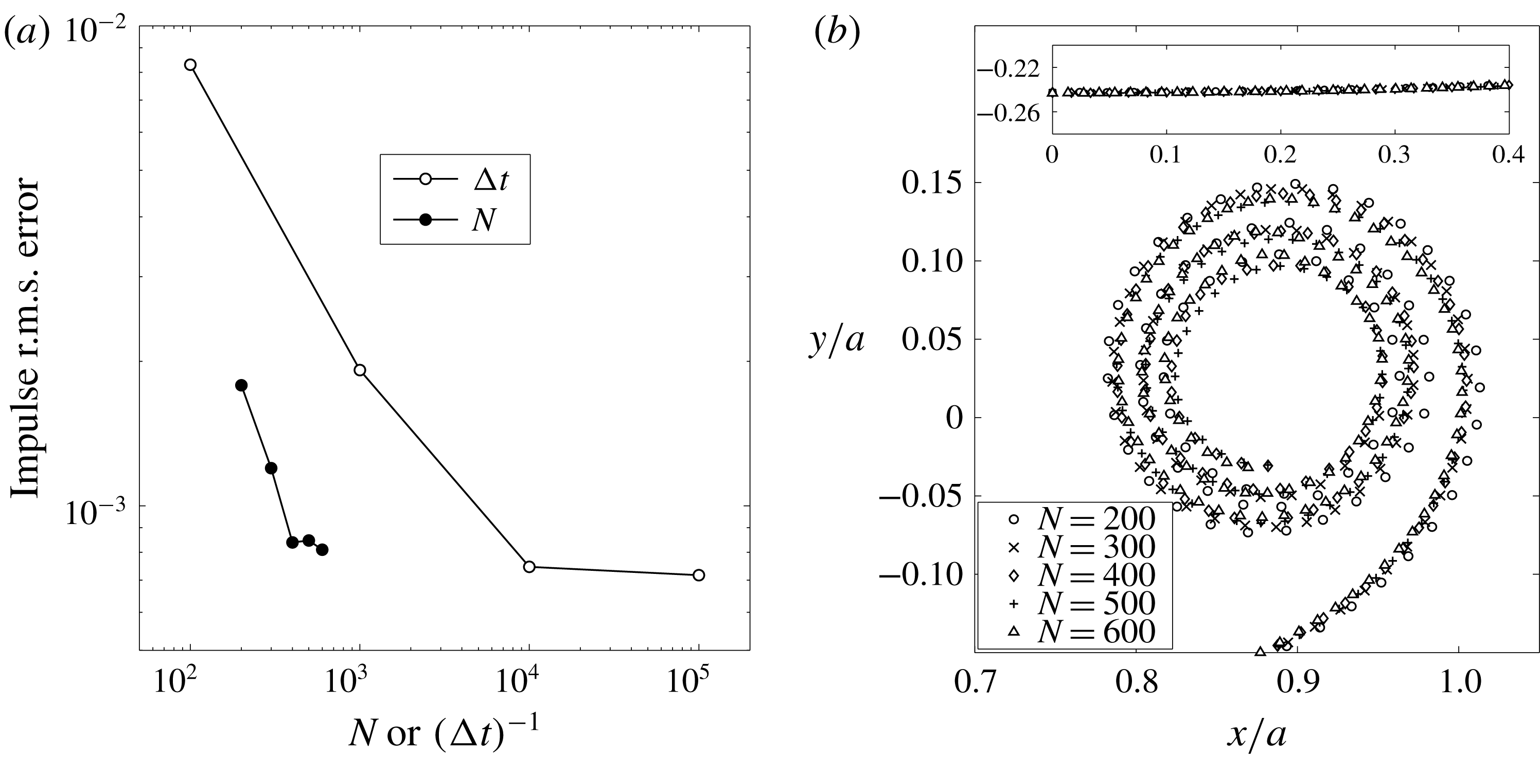
(a) The root-mean-square error over time (
 $0\leqslant t\leqslant 1$
) in the computed impulse relative to the invariant theoretical value of
 $I_{o}=\unicode[STIX]{x03C0}Ua^{2}$
for different
 $\unicode[STIX]{x0394}t$
with fixed
 $N=400$
(open circles) and different
 $N$
at fixed
 $\unicode[STIX]{x0394}t=5\times 10^{-5}$
(solid circles). (b) The sheet positions at
 $t=0.25$
for
 $N=200$
, 300, 400, 500 and 600. Only the outer turns are shown for clarity. Inset: points near the centre of the sheet away from the spiral. Data are from § 4 for a finite vortex sheet with elliptical circulation distribtuion.
3.3 Convergence
To demonstrate consistency and convergence of the proposed method we present some data from § 4 which investigate the finite vortex sheet with an elliptical circulation distribution. First, consider the vertical impulse of the sheet, which is an invariant of the motion with value
 $I_{o}=\unicode[STIX]{x03C0}Ua^{2}$
. Figure 2(a) shows the root-mean-square (r.m.s.) error of the computed impulse over time (
 $0\leqslant t\leqslant 1$
) relative to the theoretical values for several different combinations of
 $N$
and
 $\unicode[STIX]{x0394}t$
. It was verified that further increasing
 $N$
or decreasing
 $\unicode[STIX]{x0394}t$
yielded negligible differences in the computed results. Also, for the computation to remain stable, it was required that
 $\unicode[STIX]{x0394}t$
be smaller for larger
 $N$
.
Figure 2(b) plots the segment endpoints representing the rolled-up vortex sheet at
 $t=0.25$
for
 $N=200$
, 300, 400, 500 and 600 each with
 $\unicode[STIX]{x0394}t=5\times 10^{-5}$
. It is seen that the largest variations occur in the outermost turn but these decrease with increasing
 $N$
. The innermost turns were omitted for clarity; see figure 5 for an example of these closely wound turns. The inset shows sheet position near the centre symmetry plane where there is nearly no difference between each value of
 $N$
.
4 Finite vortex sheet
Here, we demonstrate the method developed in this paper on the well-known problem of the trailing-edge vortex sheet left in the wake of an elliptically loaded wing. The initial sheet position is
 $-a\leqslant x\leqslant a$
,
 $y=0$
with strength density
 $\unicode[STIX]{x1D6FE}(x)=2Ux(a^{2}-x^{2})^{-(1/2)}$
, thus giving an initial velocity of
 $u(x)=0$
,
 $v(x)=-U$
. The problem is non-dimensionalized by
 $a$
and
 $U$
giving a corresponding time
 $t=Ut_{d}/a$
. The non-dimensional quantities are implied throughout unless otherwise noted. The symmetry of the problem is taken advantage of so that
 $\unicode[STIX]{x1D6E4}_{s}$
represents the circulation in the right half of the sheet as measured from the centre. Then (3.4) must be supplemented with the integral over the left side of the sheet located at
 $z=-\overline{z}$
. Since the sheet strength is infinite at the tip, the velocities are very large there and so the rediscretization process is critical to maintaining appropriately spaced segment points. Here we use a forward Euler time-integration scheme so that the rediscretization procedure occurs after each advection of the sheet.
4.1 Validation with previous results
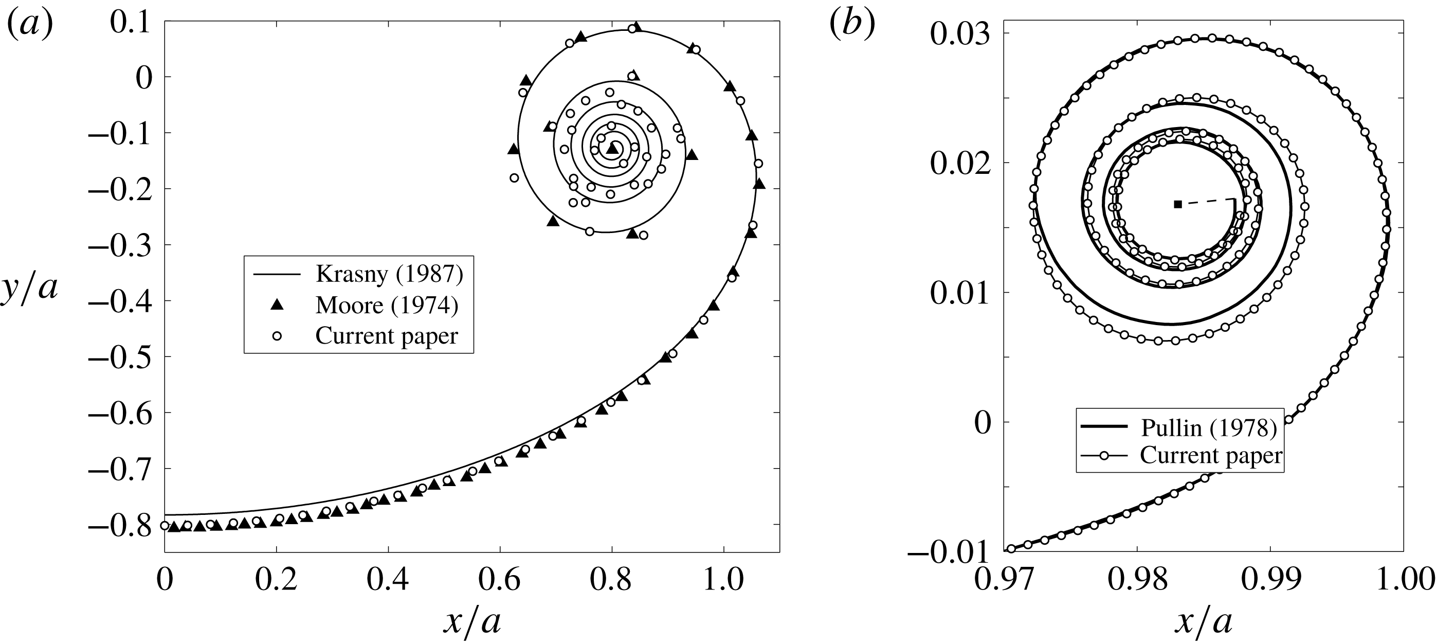
First, we attempt to produce results consistent with the point vortex methods of Moore (Reference Moore1974) and Krasny (Reference Krasny1987). This is done by omitting the self-induced velocity and neglecting curvature by removing the rediscretization process altogether. Figure 3(a) shows the comparison. We used the same numerical parameters as Moore, but with no core dumping into an isolated point tip vortex and as a result the points in the centre of the spiral began to move chaotically and lost the representation of the sheet. However, since these points represent segment endpoints and not point vortices, the calculations remained bounded and we more-or-less reproduced Moore’s data in the outer turns with the centroid of the chaotic points matching the centre of the actual spiral. We could reduce the chaotic motion by using a larger number of points and/or a smaller time step, but the purpose of this comparison was to show consistency by omitting the aforementioned effects and this point has essentially been made.
(a) Roll-up at
 $t=1$
compared with previous point vortex methods. The results of Krasny (Reference Krasny1987) were recreated with the vortex blob parameter
 $\unicode[STIX]{x1D6FF}=0.05$
,
 $N=200$
and
 $\unicode[STIX]{x0394}t=0.01$
. Moore (Reference Moore1974) used
 $N=60$
,
 $\unicode[STIX]{x0394}t=2\times 10^{-3}$
and core dumping. The current paper used the same parameters as Moore, but no core dumping, and omitted both the self-induced velocity and curvature. (b) Roll-up at
 $t=0.01$
compared with Pullin (Reference Pullin1978); the solid square is the isolated vortex at the spiral core. The current method used
 $s$
-spacing with
 $N=1000$
,
 $\unicode[STIX]{x0394}t=10^{-5}$
and includes curvature, but no self-induced velocity. Four more complete turns were computed, but were omitted for clarity.
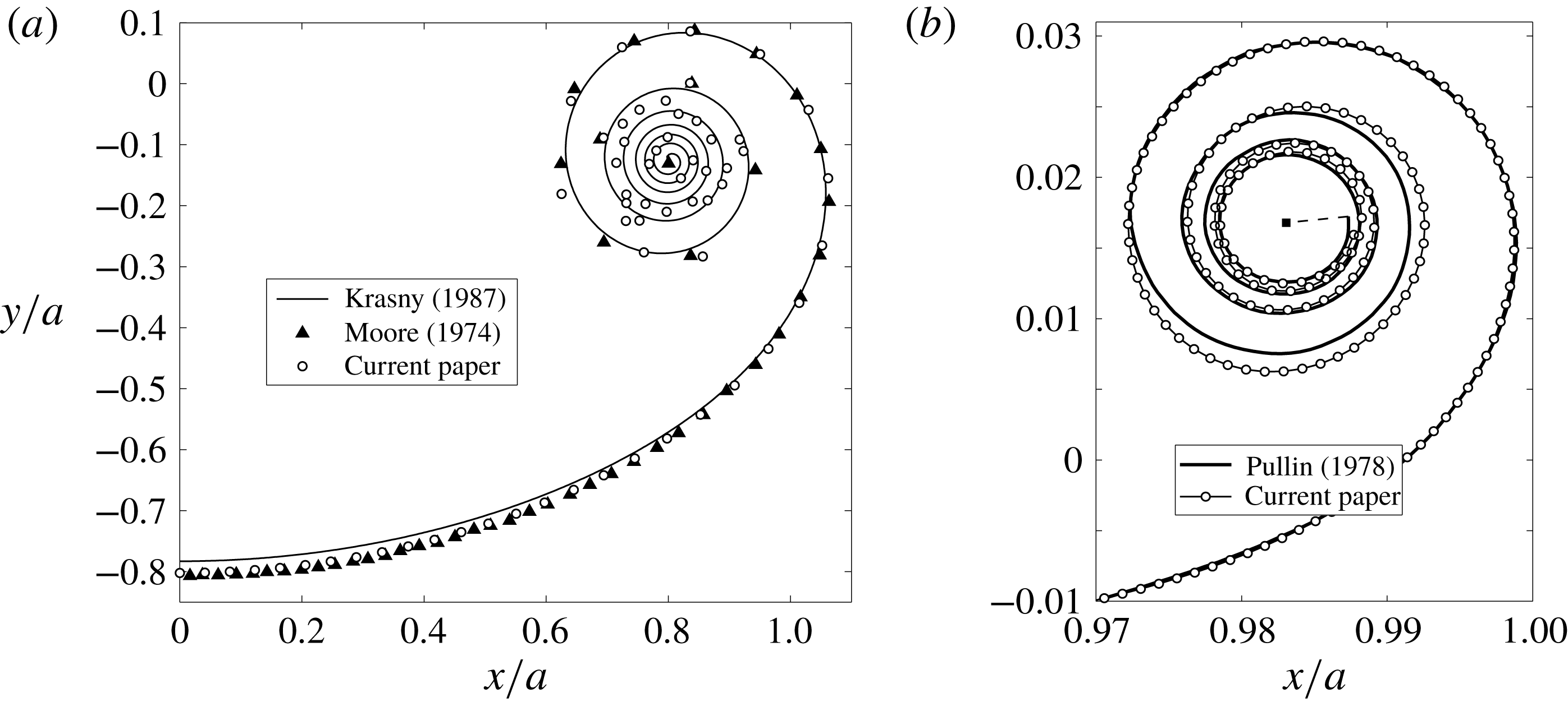
Next, we compare with the calculations of Pullin (Reference Pullin1978) for the self-similar roll-up of a semi-infinite vortex sheet; see figure 3(b). While he used straight segments and thus did not explicitly account for curvature, the resolution is very fine and represents an acceptable comparison for the effects of sheet curvature. Also, Pullin ‘ignor[ed] the Cauchy principal value singularity for
 $j=k$
’, stating that this is equivalent to assuming a linear variation of
 $\unicode[STIX]{x1D6E4}$
over that segment, or equivalently a constant
 $\unicode[STIX]{x1D6FE}$
, and gives a zero contribution. Therefore, the self-induced velocity is treated as in vortex panel methods and is not explicitly taken into account. Hence, for this simulation we reintroduce the effect of curvature, but still omit our model of the self-induced velocity. Now, to be consistent with the similarity solution we must compare at an early stage of the roll-up of the finite vortex sheet. The time
 $t=0.01$
is chosen so that the diameter of the spiral region is approximately 1.5 % of the initial sheet length of
 $2a$
. The scaling from the similarity space
 $\unicode[STIX]{x1D714}=\unicode[STIX]{x1D709}+\text{i}\unicode[STIX]{x1D702}$
to physical space
 $z=x+\text{i}y$
is
 $z=(a^{\prime }t)^{2/3}\unicode[STIX]{x1D714}$
and
 $a^{\prime }$
was chosen so that the zero-slope tangent at
 $\unicode[STIX]{x1D709}=-2.2$
in Pullin’s figure 1 was matched to our sheet at
 $x/a\approx 0.85$
, which is approximately the same number of spiral diameters away.
Figure 3(b) shows the comparison with the
 $s$
-spacing, which captures the tight outer turns of the spiral and agrees quite well with Pullin’s data who also used more-or-less equal arclength spacing. The explicit effect of curvature is seen to be greatest in the outermost turn which is farthest away from other turns. A large value of
 $N=1000$
was chosen so that several turns of the (nearly self-similar) spiral are captured at the small time
 $t=0.01$
.
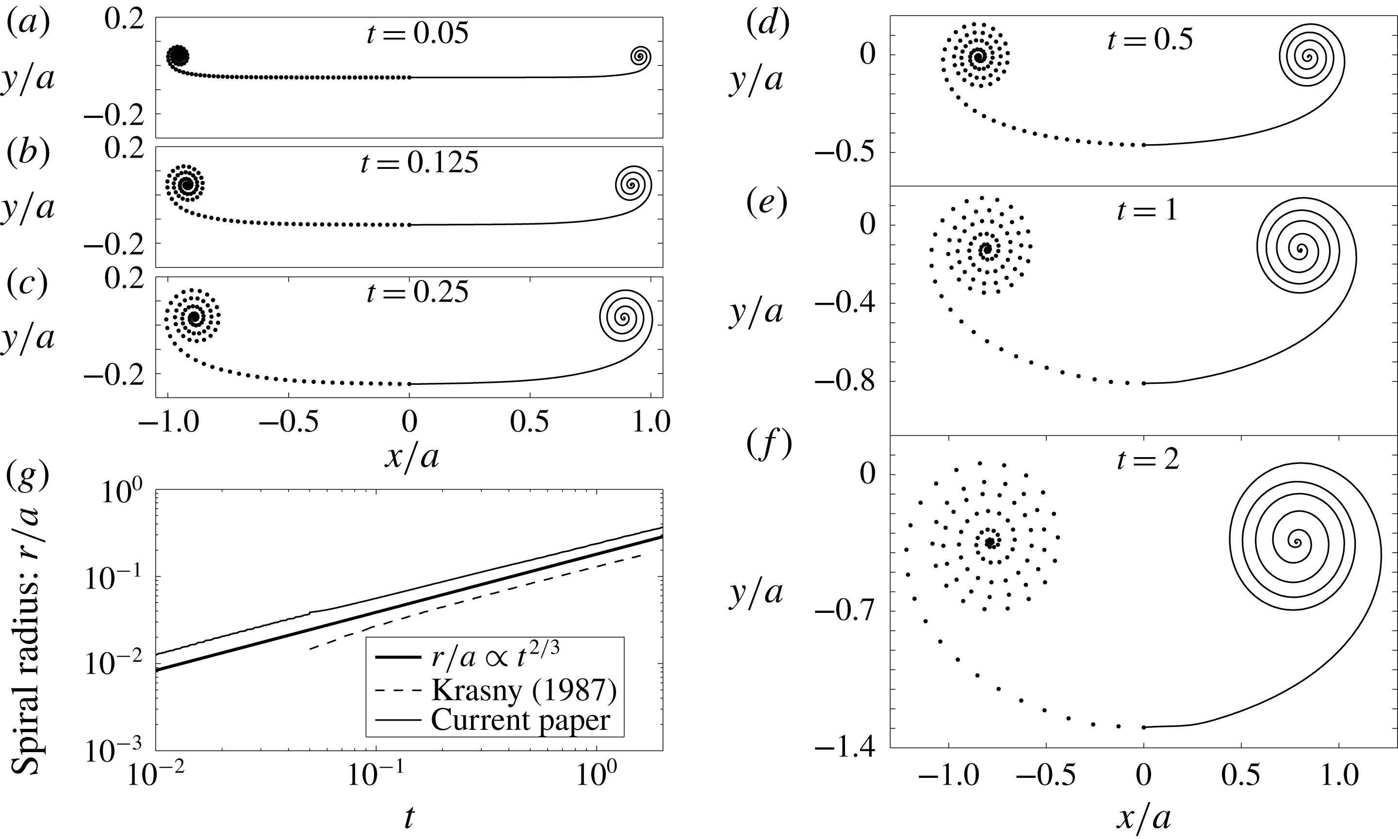
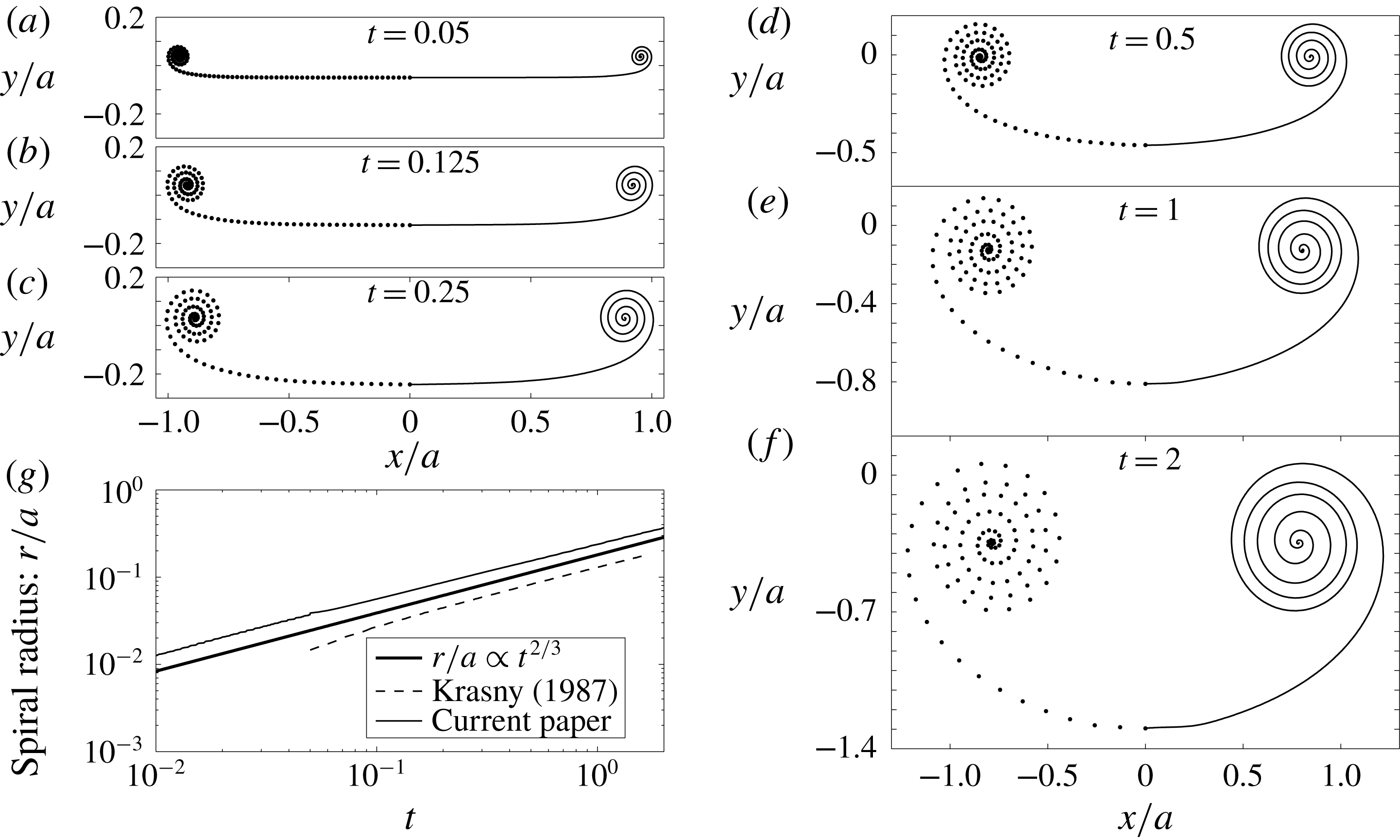
(a–f) The vortex sheet roll-up for
 $0.05\leqslant t\leqslant 2$
as indicated, including the self-induced velocity and curvature effects. The parameters are
 $N=100$
with
 $\unicode[STIX]{x1D719}$
-spacing,
 $\unicode[STIX]{x0394}t=10^{-5}$
for
 $0\leqslant t\leqslant 0.05$
and
 $\unicode[STIX]{x0394}t=10^{-3}$
for
 $0.05<t\leqslant 2$
. The segment endpoints are plotted as the left side of the sheet and the spline interpolations as the right side. (g) Log–log plot of the spiral radius growth. Also shown are the similarity relation
 $r\propto t^{2/3}$
of Kaden (Reference Kaden1931) and the recreated results of Krasny (Reference Krasny1987) with the vortex blob method.
4.2 Roll-up with the self-induced velocity
We have shown that our method can reproduce the results of previous studies by identifying and omitting the particular effects not accounted for in those calculations. Furthermore, we have given a convincing argument and derivation for an appropriate treatment of the self-induced velocity. We now present roll-up calculations that include our model for this effect.
Figure 4(a–f) shows the roll-up with
 $\unicode[STIX]{x1D719}$
-spacing at several times in the range
 $0.05\leqslant t\leqslant 2$
. Also, figure 4(g) plots the spiral radius growth and comparison with the similarity solution of Kaden (Reference Kaden1931) shows that the spiral still grows according to the
 $r\propto t^{2/3}$
similarity law. The effects of curvature and the self-induced velocity on the sheet shape result in wider turns in the spiral region as compared to Krasny (Reference Krasny1987). This is due to the stretching of the sheet by these two effects. As an analogy consider a torsional spring that is tightly wound. The potential energy stored in the spring will expand the coil back to equilibrium with wider turns when the externally applied torque on the spring is released and likewise for the vortex sheet since it cannot support a force or torque.
The
 $\unicode[STIX]{x1D719}$
-spacing always redistributes 30 % of the points in approximately the last 10 % of the sheet length near the tip. We found that the iterative rediscretization with this spacing prevented the formation of the closely spaced turns of the inner spiral by essentially unwinding them toward the very centre. Increasing the number of segments
 $N$
puts so many points near the centre that numerical errors quickly accumulated. Hence, for further discussion we employ the
 $s$
-spacing, for which an example of the sheet shape at
 $t=0.25$
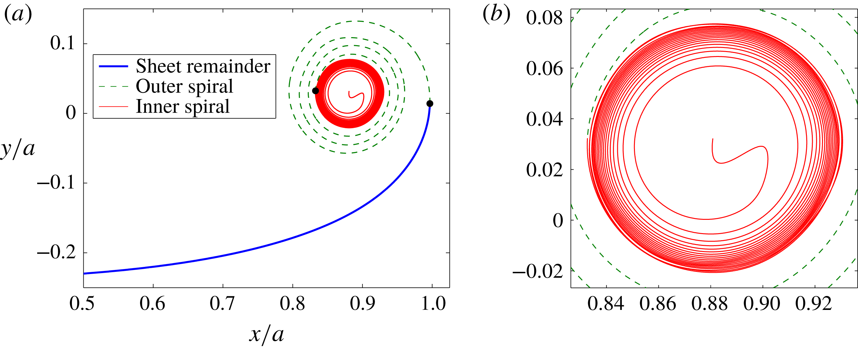
is shown in figure 5(a). The outermost turn matches with the
 $\unicode[STIX]{x1D719}$
-spacing (not shown), however the
 $s$
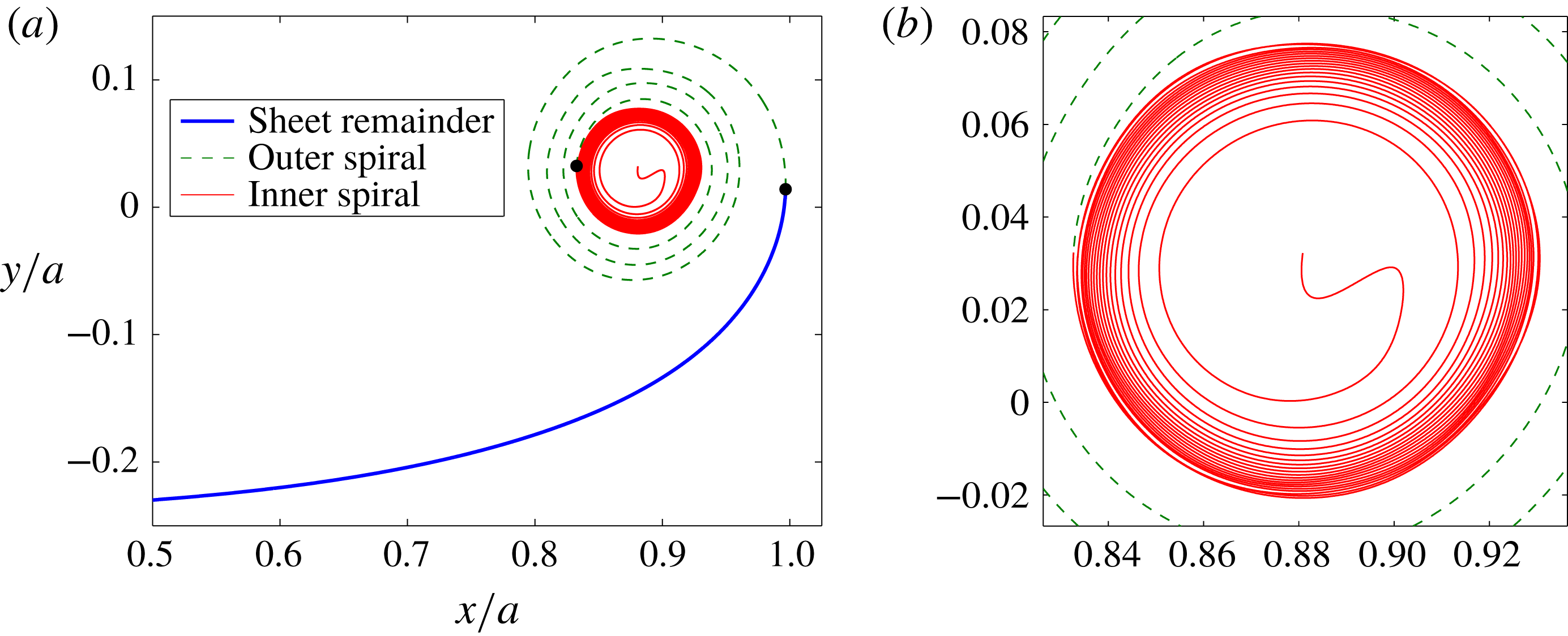
-spacing shows closer turns further within the spiral which become very tight, but these do not extend to the centre of the spiral; the reason for this will be explained later. In this plot we also define different regions of the sheet where the unrolled ‘sheet remainder’ extends from the centre of the sheet to the most extraneous
 $x$
-coordinate (i.e. infinite slope), the ‘outer spiral’ corresponds to the turns that occur between this point and the ‘inner spiral’ that begins where the outer spiral is tangent to the very tightly wound turns; see figure 5(b).
(a) Roll-up at
 $t=0.25$
with the
 $s$
-spacing and
 $N=600$
. The solid dots represent locations defining different regions of the sheet as indicated; see text. (b) Zoomed-in view of the inner spiral region of (a). There are 20 total turns with approximately 3 in the outer spiral and 17 in the inner spiral and the total arclength is 8 times the initial sheet length.
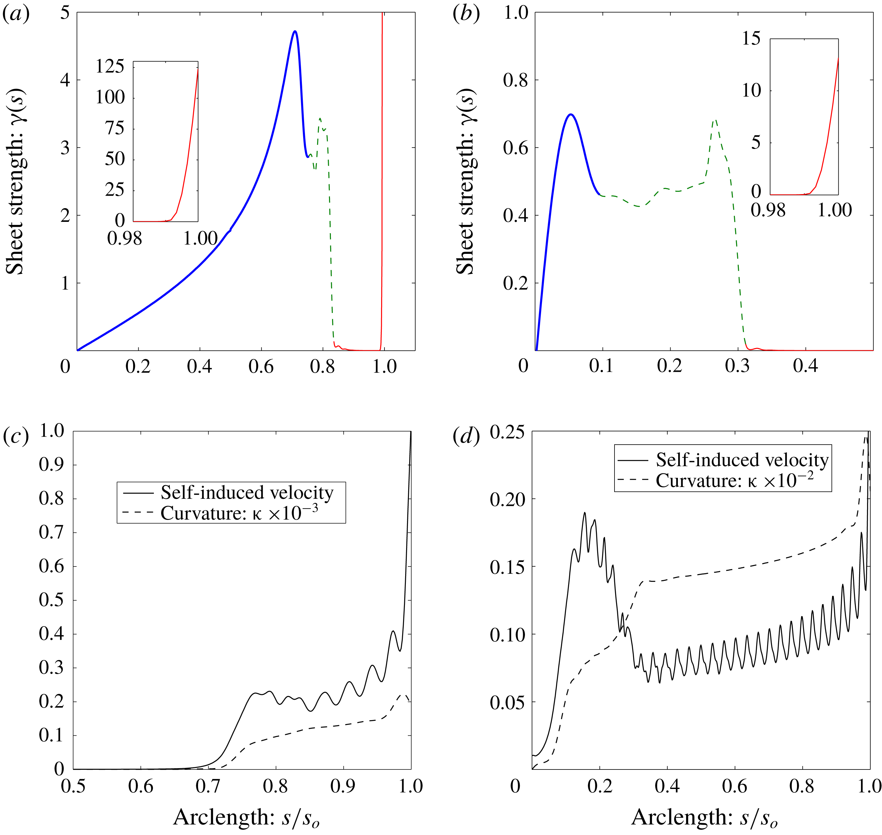
(a,b) The vortex sheet strength
 $\unicode[STIX]{x1D6FE}(s)$
along the sheet coordinate normalized by the total arclength
 $s_{o}$
for (a)
 $t=0.01$
,
 $s_{o}=1.34a$
and (b)
 $t=0.5$
,
 $s_{o}=12.58a$
. The line/colour styles correspond to the regions of the sheet defined in figure 5(a). The insets show
 $\unicode[STIX]{x1D6FE}$
very near the tip of the sheet. (c,d) The magnitude of the self-induced velocity
 $q_{s}$
normalized by the sheet-averaged total velocity magnitude and the sheet curvature
 $\unicode[STIX]{x1D705}$
for (c)
 $t=0.01$
,
 $s_{o}=1.34a$
and (d)
 $t=0.5$
,
 $s_{o}=12.58a$
.
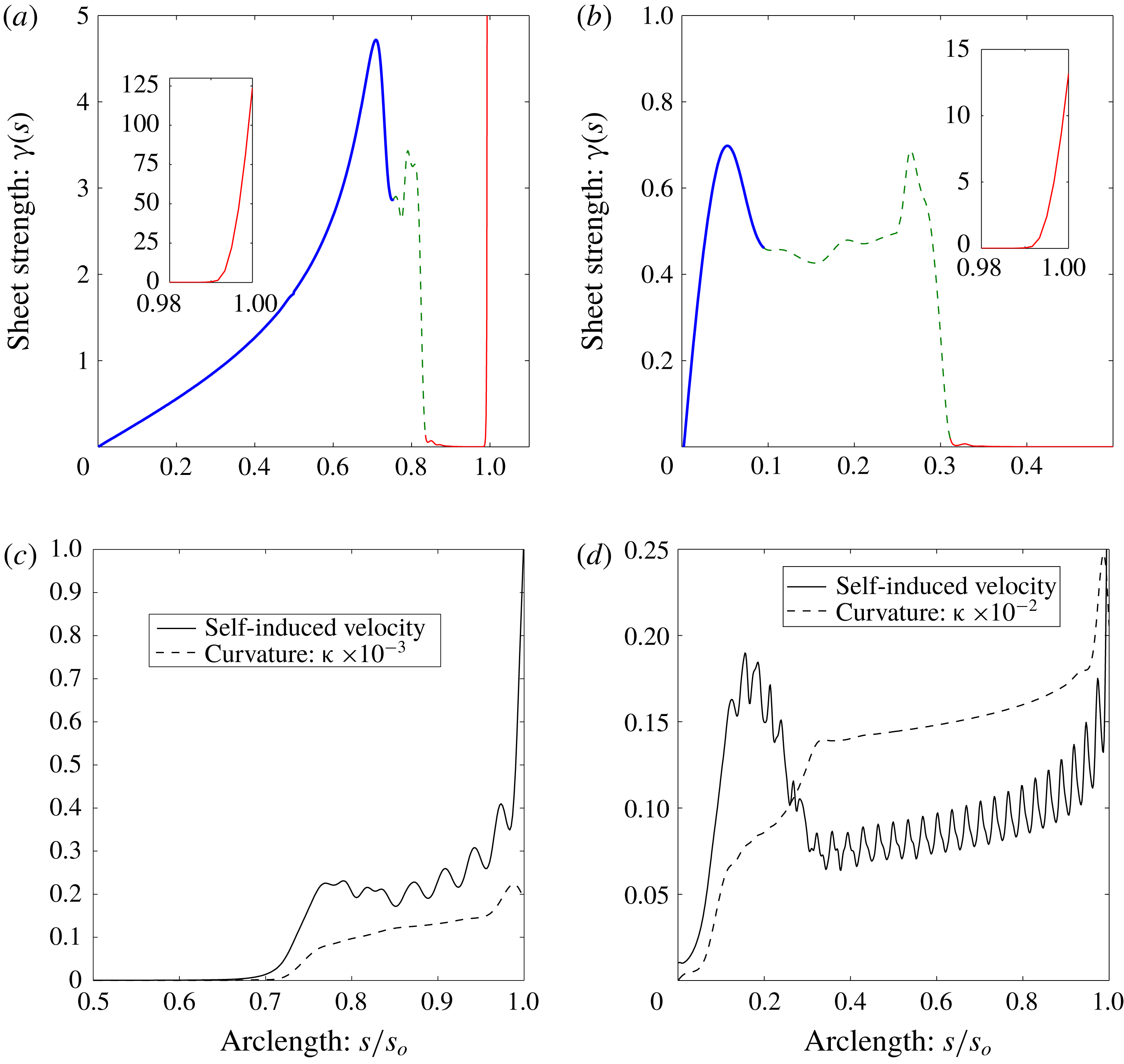
The initial vortex sheet strength is singular at the tip of the sheet, which results in an infinite velocity there that begins the roll-up process. While formulating the problem in terms of
 $\unicode[STIX]{x1D6E4}$
preserves the total circulation, the infinite velocity cannot be captured numerically. Figure 6(a,b) shows
 $\unicode[STIX]{x1D6FE}(s)$
along the sheet at the times
 $t=0.01$
and
 $t=0.5$
, respectively. We see that very early on
 $\unicode[STIX]{x1D6FE}$
is ‘split’ with a small portion of the circulation (here 7 %) going very near the sheet tip, which essentially corresponds to the isolated vortex that other researchers have used to represent the innermost portion of the spiral (e.g. Moore Reference Moore1974, Fink & Soh Reference Fink and Soh1978, Pullin Reference Pullin1978). The rest of the circulation is spread along the sheet remainder and the outer spiral. The inner spiral has essentially no strength density, but as roll-up proceeds the total arclength
 $s_{o}(t)$
is significantly increased in this region where the sheet is stretched by the tip. The inset plots show that the portion of
 $\unicode[STIX]{x1D6FE}$
in the sheet tip is spread out over more of the innermost turn as
 $t$
increases thus decreasing its maximum value as well as its gradient; note
 $s_{o}(0.01)=1.34a$
and
 $s_{o}(0.5)=12.58a$
.
Figure 6(c,d) plots the magnitude of the self-induced velocity, say
 $q_{s}$
, as well as the sheet curvature
 $\unicode[STIX]{x1D705}$
for the same times. To give perspective to
 $q_{s}$
, the average over the sheet of the magnitude of the total induced velocity is used as a normalization. The oscillations in
 $q_{s}$
are due to the fact that, at periodic positions along the spiral,
 $q_{s}$
is in-and-out of phase with the overall downward velocity of the sheet. At
 $t=0.01$
the sheet remainder is nearly flat away from the spiral and is moving normal to itself so that both
 $q_{s}$
and
 $\unicode[STIX]{x1D705}$
are zero. However, both of these quantities become non-negligible in the outer and inner spiral regions (note
 $\unicode[STIX]{x1D705}$
has been scaled down for the plots) and both increase as the spiral centre is approached. Hence, the self-induced velocity is also important in areas of high curvature despite the near-zero strength density of the inner spiral. At the sheet tip,
 $q_{s}$
sharply increases and is the dominant velocity there. Therefore, the self-induced velocity is critical in initiating the roll-up process and an artificial tip displacement to begin the process (e.g. Sugioka & Widnall Reference Sugioka and Widnall1985) is not required. Again appealing to analogy, the sheet tip is like the locomotive car of a train that pulls along its ‘passenger sheet’ while also stretching it since the tip moves with larger velocity and
 $\unicode[STIX]{x2202}\unicode[STIX]{x1D6FE}/\unicode[STIX]{x2202}s$
is very steep; recall (2.11).
The curvature shows a rapid, but smooth increase from the sheet remainder region into the outer spiral. In the inner spiral region
 $\unicode[STIX]{x1D705}$
shows a slower increase corresponding to the nearly circular turns of gradually smaller radii; this is more obvious at
 $t=0.5$
where the inner spiral has about 20 turns. It is generally accepted that vortex sheets develop curvature singularities, as was shown by Moore (Reference Moore1979) (among many others, subsequently) for the Kelvin–Helmholtz instability of an infinite vortex sheet. For the finite vortex sheet, the infinite velocity at the sheet tip results in an infinite number of turns whose radii/curvature approach zero/infinity at the very centre of the spiral. Since, as mentioned above, the numerical method cannot capture this in its entirety, then the void in the very inner spiral (recall figure 5
a) is a result of only being able to resolve a finite portion of the infinite velocity of our ‘locomotive’ at
 $t=0^{+}$
.
4.3 An impulse-conserving tip vortex
As mentioned previously, an infinite vortex sheet strength presents some numerical difficulties. Inviscid theory predicts that the infinite velocity at the free end of the sheet will immediately roll-up into a vanishingly small spiral containing an infinite number of turns. So long as
 $N<\infty$
and/or
 $\unicode[STIX]{x0394}t>0$
then there is some distribution of sheet strength (i.e. vorticity) within the core that we cannot resolve. Although circulation is conserved via the Lagrangian formulation
 $\text{d}\unicode[STIX]{x1D6E4}=\unicode[STIX]{x1D6FE}\,\text{d}s$
, we will not numerically conserve (vertical) impulse,
 $\text{d}I=x\unicode[STIX]{x1D6FE}$
, since there is a distribution of this quantity within the core as well. The method of core dumping, as employed by Moore (Reference Moore1974) for point vortices, conserves impulse by locating the new amalgamated vortex at the circulation centroid, but this occurs as dictated by a user-defined criterion. Pullin (Reference Pullin1978) approximated the core with an isolated point tip vortex and averaged the governing equation over this region. The assumptions made in the averaging are tantamount to equating the core impulse with that of the tip vortex and to defining the vortex velocity to be the average velocity within the core. Even when we attempted to maintain the tip as part of a continuous sheet, the result was a large portion of circulation at the very tip of the sheet that drives the roll-up (recall figure 6). This leaves a void in the centre of the spiral.
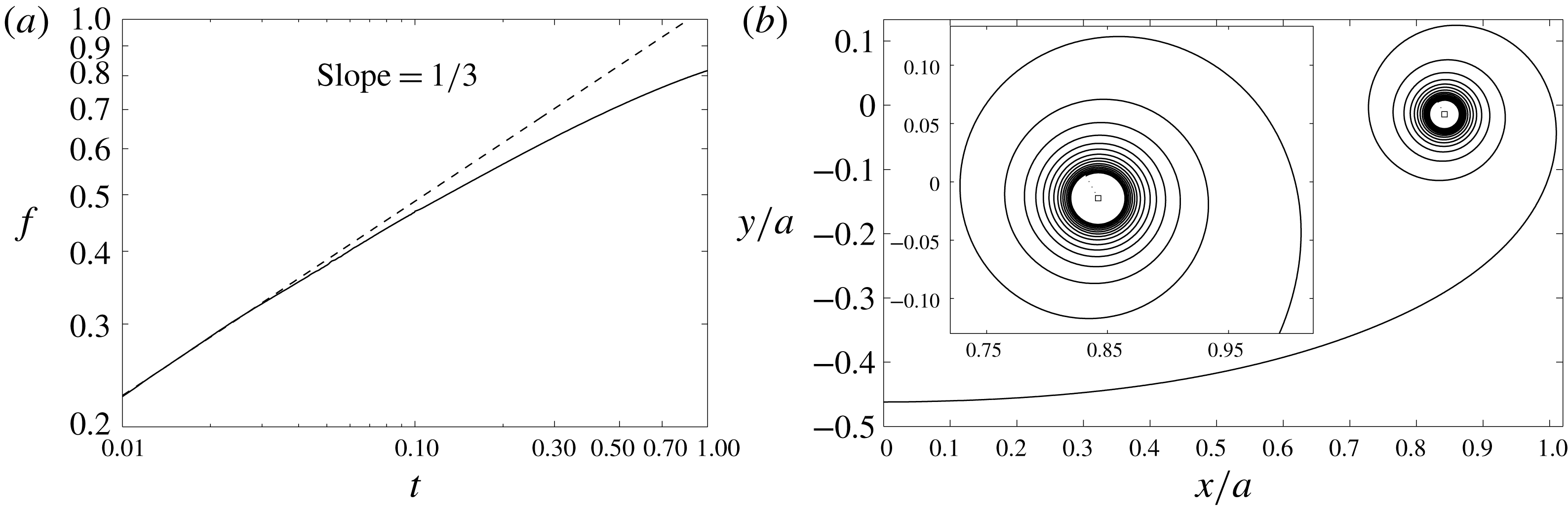
We now attempt to resolve more turns further within the spiral by adopting a similar approach as Pullin and let the
 $(N+1)$
point be an isolated vortex with position
 $z_{v}=z_{N+1}$
and circulation
 $\unicode[STIX]{x1D6E4}_{v}=\unicode[STIX]{x1D6E4}_{N+1}-\unicode[STIX]{x1D6E4}_{N}$
. The induced velocity field now contains an explicit tip vortex term:
 $$\begin{eqnarray}\displaystyle u-\text{i}v=\frac{1}{2\unicode[STIX]{x03C0}\text{i}}\left[\int _{0}^{\unicode[STIX]{x1D6E4}_{N}}\frac{\text{d}\unicode[STIX]{x1D6E4}^{\prime }}{z-z^{\prime }}+\frac{\unicode[STIX]{x1D6E4}_{v}}{z-z_{v}}+\int _{\unicode[STIX]{x1D6E4}_{N}}^{\unicode[STIX]{x1D6E4}_{N+1}}\frac{\text{d}\unicode[STIX]{x1D6E4}^{\prime }}{z-z^{\prime }}\right]. & & \displaystyle\end{eqnarray}$$
The last integral might as well be termed the self-induced velocity of the core
 $q_{v}$
and it is interesting to note that:
 $$\begin{eqnarray}q_{v}=\frac{\unicode[STIX]{x1D6E4}_{v}}{2\unicode[STIX]{x03C0}\text{i}}\left[\frac{1}{\unicode[STIX]{x1D6E4}_{v}}\int _{\unicode[STIX]{x1D6E4}_{N}}^{\unicode[STIX]{x1D6E4}_{N+1}}\frac{\text{d}\unicode[STIX]{x1D6E4}^{\prime }}{z_{v}-z^{\prime }}\right]\approx \text{i}\frac{\unicode[STIX]{x1D6E4}_{v}}{2\unicode[STIX]{x03C0}r_{c}},\end{eqnarray}$$
where
 $r_{c}^{-1}=\overline{(z-z_{v})^{-1}}$
, with the bar being an average here, is the mean inverse radius from
 $z_{v}$
to a point in the core. However, we do not attempt to calculate this here.
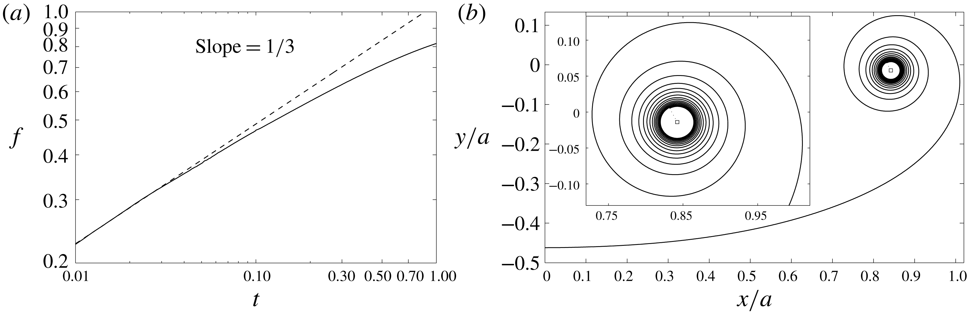
(a) The fraction
 $f$
of circulation contained within the rolled-up portion of the sheet (vortex plus outer turns). The dashed line is Kaden’s similarity law. Here
 $N=600$
and the vortex acquired circulation from the sheet until
 $t=t_{v}=0.1$
(see (4.3)) at which time
 $\unicode[STIX]{x1D6E4}_{v}/\unicode[STIX]{x1D6E4}_{s}=0.33$
. (b) The interpolated sheet shape at
 $t=0.5$
when
 $f=0.71$
so that 38 % of the circulation resides in the resolved turns. Inset: zoomed-in view of spiral region; the square symbol is the location of the vortex.
The impulse can be written as contributions from the sheet and tip vortex:
 $I=I_{s}+I_{v}$
where
 $I_{s}=\int _{0}^{\unicode[STIX]{x1D6E4}_{N}}x\,\text{d}\unicode[STIX]{x1D6E4}$
and
 $I_{v}=x_{v}\unicode[STIX]{x1D6E4}_{v}$
. We assume that after each advection of the sheet the points are in the correct positions, but the vortex will have acquired some circulation
 $\unicode[STIX]{x0394}\unicode[STIX]{x1D6E4}_{v}$
such that the impulse is conserved with the initial value
 $I_{o}$
. Therefore:
 $$\begin{eqnarray}\unicode[STIX]{x0394}\unicode[STIX]{x1D6E4}_{v}=\frac{|I_{o}-I_{s}|}{x_{v}}-\unicode[STIX]{x1D6E4}_{v},\end{eqnarray}$$
and this amount is put into the tip vortex by removing a section of the sheet near the tip with the same circulation. This is accomplished using the interpolants approximating the sheet shape and circulation as functions along the arclength. As expected, this process very quickly accumulates circulation into the tip vortex; for Pullin’s similarity solution, approximately 50 % of the circulation within the rolled-up portion of the sheet is in the vortex whereas the other 50 % is in the first four outer turns. While this process conserves impulse and allows the sheet to form initial outer turns around the growing vortex, it does not conserve energy and in fact consumes some amount of the initial energy. This represents, in a purely qualitative manner and not physically, the diffusion of the tightly wound inner spiral into a viscous core. Therefore, the amalgamation process is only allowed to occur for some small initial time
 $0<t_{v}\ll 1$
and once this has concluded the energy remains fairly constant.
The rediscretization and interpolation only apply to the
 $n=1\ldots N$
points. Also, the sheet strength at the point
 $z_{N}$
is decreased as circulation is consumed by the tip vortex. Therefore, the rediscretization process, while still important, can be implemented after the last stage of a fourth-order Runge–Kutta integration scheme. Because of the singularity, the amount of circulation acquired in the vortex will depend on
 $N$
and
 $t_{v}$
. We do not perform a detailed study of these parameters here, but we find that they mainly influence the number of turns that appear in the spiral at a later time.
Following Moore (Reference Moore1974)
 $f$
is the fraction of circulation in the rolled-up region (vortex plus outer turns) and is plotted in figure 7(a) for the case with
 $N=600$
and
 $t_{v}=0.1$
at which time
 $f=0.47$
and
 $\unicode[STIX]{x1D6E4}_{v}/\unicode[STIX]{x1D6E4}_{s}=0.33$
so 14 % of the circulation is contained in the outer turns. The sheet shape at
 $t=0.5$
obtained from this procedure is shown in figure 7(b). At this time
 $f=0.71$
so that now approximately 38 % of the circulation resides in the outer turns. The results are remarkably similar to those of Moore (Reference Moore1974) and Krasny (Reference Krasny1986a
). While there is still a small void in the centre, this can be made smaller by decreasing
 $t_{v}$
. Many more turns can be captured at a given time, but at the expense of smaller time steps to accurately evolve the sheet and avoid the accumulation of errors.
5 Infinite vortex sheet
In this section we investigate the Kelvin–Helmholtz instability arising from a periodically disturbed infinite vortex sheet. Unlike the finite vortex sheet, the sheet strength and velocities are initially bounded so that the rediscretzation process is less crucial than in § 4. Therefore, we use a fourth-order Runge–Kutta scheme throughout and the rediscretization is performed after the last stage. For reasons discussed below, the sheet is considered as two halves separated by the midpoint where the singularities form. In this way, the rediscretization is applied to each half individually so that no interpolation occurs through the singularity point.
If
 $\unicode[STIX]{x1D706}$
is the wavelength of the disturbance then the infinite integration bounds in (1.1) can be reduced to:
 $$\begin{eqnarray}u-\text{i}v=\frac{1}{2\unicode[STIX]{x1D706}\text{i}}\int _{0}^{\unicode[STIX]{x1D6E4}_{s}}\cot \left[\frac{\unicode[STIX]{x03C0}}{\unicode[STIX]{x1D706}}(z-z^{\prime })\right]\text{d}\unicode[STIX]{x1D6E4}^{\prime },\end{eqnarray}$$
where it is implied that
 $z=z(\unicode[STIX]{x1D6E4})$
and
 $\unicode[STIX]{x1D6E4}_{s}$
is the total circulation in one period. The initial condition of the sheet is characterized by a disturbance amplitude
 $\unicode[STIX]{x1D716}$
. The disturbance types that have been most studied are perturbations to the initial sheet shape and to the initial circulation/strength distribution. It is well known that the perturbed sheets develop singularities in a finite critical time
 $t_{c}$
at which the solution to (5.1) ceases to be analytic. Moore (Reference Moore1979) used an asymptotic analysis of the Fourier coefficients of a transverse sinusoidal disturbance of the sheet shape to derive an estimate for the dependence of
 $t_{c}$
on
 $\unicode[STIX]{x1D716}$
. The singularity is an infinite jump discontinuity of the sheet curvature at the point around which roll-up would occur.
Krasny (Reference Krasny1986b
) adapted Moore’s relation of
 $t_{c}(\unicode[STIX]{x1D716})$
for the initial condition of a purely growing mode and used the point vortex method to investigate the singularity formation. Meiron, Baker & Orszag (Reference Meiron, Baker and Orszag1982) considered a sinusoidal perturbation to the circulation distribution of an initially flat sheet and also adapted Moore’s analysis, which for larger amplitudes slightly underpredicts their critical time determined from analysis of a temporal Taylor series. Higdon & Pozrikidis (Reference Higdon and Pozrikidis1985) studied the same problem using a discrete method where the sheet is comprised of interpolated circular arcsegments and the sheet strength is a piecewise trigonometric function; they also implemented a point-insertion procedure. All groups agree on the curvature singularity, but there is some disagreement about other aspects of the singularity.
Moore (Reference Moore1979) notes that at the critical time the sheet is only slightly deformed and does not exhibit features of roll-up. The sheet profiles computed by Meiron et al. (Reference Meiron, Baker and Orszag1982) agree with this and they also show that at
 $t_{c}$
the sheet strength exhibits a finite cusp. Krasny (Reference Krasny1986b
) also came to the conclusion of a finite cusp at
 $t_{c}$
. He also mentions that D. I. Pullin has conjectured that the vortex sheet rolls up from both sides of the singularity and forms a double-branched spiral with an infinite number of turns and the size of which vanishes as
 $t\rightarrow t_{c}^{+}$
. This would suggest that
 $\unicode[STIX]{x1D6FE}$
is also infinite for
 $t>t_{c}$
, as claimed by Higdon & Pozrikidis (Reference Higdon and Pozrikidis1985) who numerically computed initial stages of roll-up from which they inferred that
 $\unicode[STIX]{x1D6FE}$
is also infinite at
 $t=t_{c}$
.
Here, we attempt to resolve this discrepancy concerning the vortex sheet strength for
 $t\geqslant t_{c}$
and the rolling-up of the sheet. We analyse the same problem as Krasny (Reference Krasny1986b
) for which the initial condition is:
 $$\begin{eqnarray}z(\unicode[STIX]{x1D6E4},0)=\unicode[STIX]{x1D6E4}+\unicode[STIX]{x1D716}(1-i)\sin 2\unicode[STIX]{x03C0}\unicode[STIX]{x1D6E4},\end{eqnarray}$$
with constant sheet strength
 $\unicode[STIX]{x1D6FE}=\text{d}\unicode[STIX]{x1D6E4}/\text{d}s$
and
 $\unicode[STIX]{x1D716}=0.01$
; for simplicity let
 $\unicode[STIX]{x1D706}=1=\unicode[STIX]{x1D6E4}_{s}$
. Krasny found two types of irregular point vortex motions: one occurring at small times due to spurious growth of round-off errors and another occurring beyond the critical time where the accuracy of the time integration suffers. Considering the former, he proposed a filtering of the point positions to prevent unphysical growth and obtained regular motion for
 $t<t_{c}$
. For the current method the first type of error in the sheet position can be attenuated by the interpolation in the rediscretization process. Next, we first describe the determination of the critical time.
5.1 The critical time
$t_{c}$

By definition the sheet is analytic up to the critical time so that the spline interpolation, which has continuous and bounded curvature, should be able to appropriately approximate the true sheet shape prior to
 $t_{c}$
. Also, by treating each half of the sheet separately the jump in curvature at the midpoint can be captured. We found that rediscretizing the points to equal arclength segments results in insufficient resolution upon approaching the critical time, as was similarly noted by Higdon & Pozrikidis (Reference Higdon and Pozrikidis1985). However, the behaviour was interesting: the circulation as a function of arclength developed a finite jump discontinuity at the singularity point indicating the amount of circulation that would be rolled-up into the double-branched spiral. Nevertheless, the rediscretization was instead performed to segments of equal circulation. This is similar to a point vortex method, but is distinctly different because the points are connected via the rediscretization and the total arclength of the sheet increases as it evolves.
(a) The time
 $t_{\unicode[STIX]{x1D6FE}}^{N}$
at which
 $\text{d}\unicode[STIX]{x1D6FE}/\text{d}s$
becomes monotonic on each side of the midpoint indicating a cusp in
 $\unicode[STIX]{x1D6FE}(s)$
for
 $\unicode[STIX]{x1D716}=0.01$
. The line is a first-order linear least squares fit to the data. (b) The maximum curvature
 $\unicode[STIX]{x1D705}_{max}$
and its inverse as functions of time for a computation with
 $N=400$
. The bold vertical line is the estimated critical time
 $t_{c}=0.404$
as predicted in § 5.1. (c)
 $t_{c}$
versus
 $\unicode[STIX]{x1D716}$
(left axis). Also shown are the results of Krasny (Reference Krasny1986b
) and the asymptotic relation he derived from the method of Moore (Reference Moore1979); see (5.3). The vortex sheet strength at the critical time
 $\unicode[STIX]{x1D6FE}_{c}$
(right axis).

Higdon & Pozrikidis (Reference Higdon and Pozrikidis1985) used the inverse of the maximum curvature,
 $\unicode[STIX]{x1D705}_{max}(t)$
, tending toward zero to estimate the critical time. Determining
 $t_{c}$
in this way, while not necessarily inaccurate, is somewhat arbitrary as we find that the computation of this quantity monotonically increases, which prevents an objective determination of
 $t_{c}$
. Krasny (Reference Krasny1986b
) used a criterion based on the time at which a straight line interpolant between the point vortices immediately adjacent to the midpoint obtained a vertical slope. Several separate computations with different values of
 $N$
were performed in order to extrapolate to
 $N\rightarrow \infty$
. We adopt Krasny’s method of extrapolation, but using a different quantity. Namely, if
 $\unicode[STIX]{x1D6FE}(s,t)$
forms a cusp at
 $s=s_{c}$
and
 $t=t_{c}$
, then
 $\unicode[STIX]{x2202}\unicode[STIX]{x1D6FE}/\unicode[STIX]{x2202}s$
ought to be monotonic for
 $|s-s_{c}|>0$
. Therefore,
 $t_{\unicode[STIX]{x1D6FE}}^{N}$
is defined as the time when
 $\unicode[STIX]{x2202}\unicode[STIX]{x1D6FE}/\unicode[STIX]{x2202}s$
first becomes monotonic over the half-sheet; the calculation excludes the midpoint.
We computed solutions with
 $N$
ranging from 150 to 400 and time step
 $\unicode[STIX]{x0394}t=0.001$
; below
 $N=150$
there was insufficient spatial resolution to compute
 $\unicode[STIX]{x2202}\unicode[STIX]{x1D6FE}/\unicode[STIX]{x2202}s$
. Prior to the critical time the mean difference in the interpolated sheet shapes,
 $|\unicode[STIX]{x0394}z|$
, for increments of
 $\unicode[STIX]{x0394}N=100$
went from
 $|\unicode[STIX]{x0394}z/\unicode[STIX]{x1D716}|\sim O(10^{-3})$
to
 ${\sim}O(10^{-4})$
. It was also verified that the results were converged with time step upon comparison with
 $\unicode[STIX]{x0394}t=0.0001$
. Following Krasny, a polynomial in
 $N^{-1}$
is fit to the data for
 $t_{\unicode[STIX]{x1D6FE}}^{N}$
, but since we have
 $N^{-1}\sim O(10^{-3})$
we only take a first-order fit:
 $t_{\unicode[STIX]{x1D6FE}}^{N}\approx t_{\unicode[STIX]{x1D6FE}}^{\infty }+c_{1}N^{-1}$
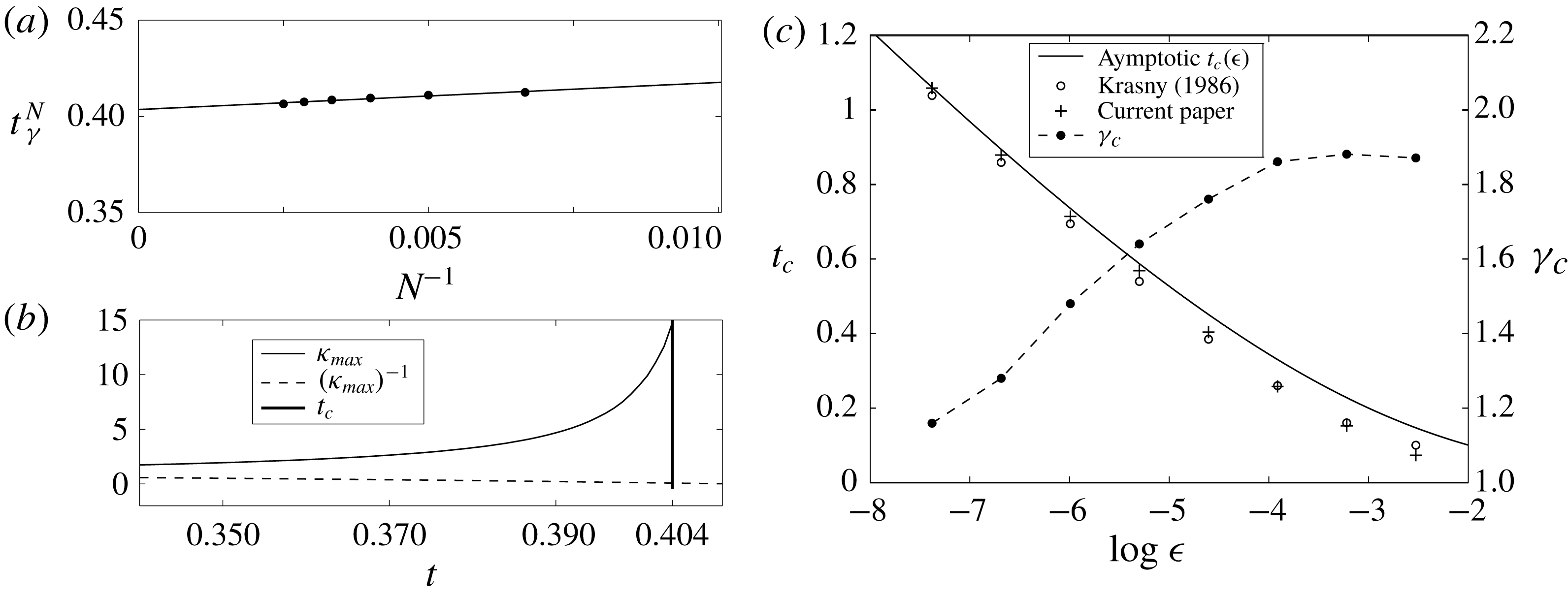
. Figure 8(a) shows the data points for
 $\unicode[STIX]{x1D716}=0.01$
and the fitted line, which gives an estimated critical time of
 $t_{c}=0.404$
. This is larger than that predicted by Krasny (
 $t_{c}=0.375$
), but closer to the value of 0.451 he obtained through the asymptotic method of Moore (Reference Moore1979). As an a posteriori consistency check on the value of
 $t_{c}$
predicted here, figure 8(b) plots
 $\unicode[STIX]{x1D705}_{max}$
and its inverse (minimum radius of curvature) with the bold vertical line marking
 $t_{c}=0.404$
and we see that
 $t_{c}$
occurs when the computed curvature is rapidly increasing as expected.
The above procedure was applied to the same range of amplitudes investigated by Krasny, namely
 $0.000625\leqslant \unicode[STIX]{x1D716}\leqslant 0.08$
, and the results are plotted figure 8(c). Also shown is the asymptotic relation for
 $\unicode[STIX]{x1D716}\ll 1$
, which is given by:
 $$\begin{eqnarray}\unicode[STIX]{x03C0}t_{c}+1+\log \unicode[STIX]{x03C0}t_{c}=\log \frac{1}{2\unicode[STIX]{x03C0}\unicode[STIX]{x1D716}}.\end{eqnarray}$$
For small amplitudes the
 $t_{c}$
predicted here are seen to align more with the asymptotic relation, but for larger amplitudes the critical time becomes shorter. We interpret these to be effects of representing the sheet as a continuous object. Namely, for small
 $\unicode[STIX]{x1D716}$
the disturbance is dampened by nonlinear stretching of the sheet, whereas for larger
 $\unicode[STIX]{x1D716}$
nonlinear excitation amplifies the disturbance (Moore Reference Moore1979). Also plotted in figure 8(c) is the computed vortex sheet strength at the singularity
 $\unicode[STIX]{x1D6FE}_{c}=\unicode[STIX]{x1D6FE}(s_{c},t_{c})$
, which supports the intuitive trend that larger disturbance amplitudes transport more vorticity toward the midpoint resulting in earlier critical times and roll-up.
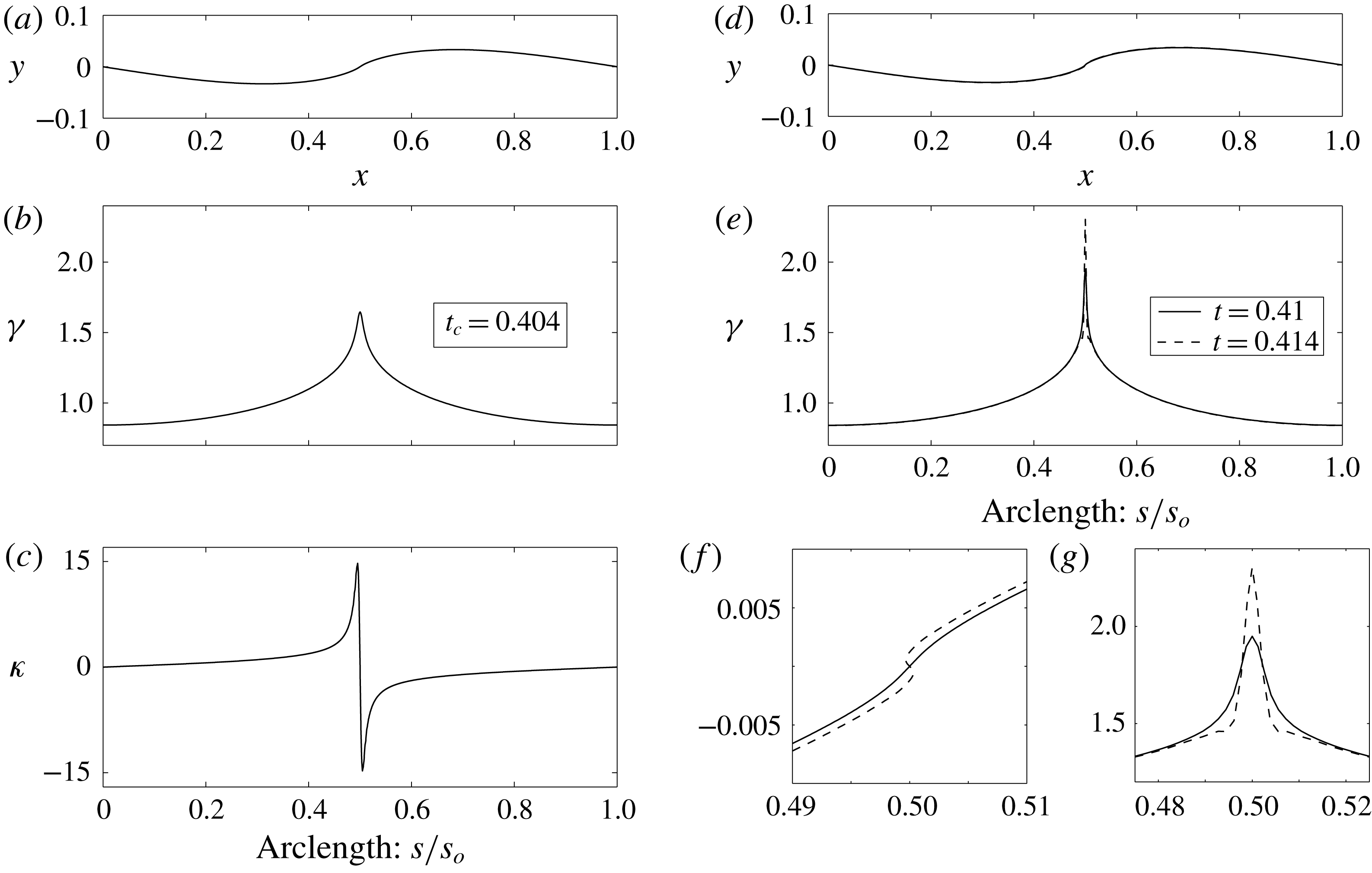
(a–c) The solution with
 $N=400$
at the estimated critical time
 $t_{c}=0.404$
. (a) Interpolated sheet position, (b) vortex sheet strength
 $\unicode[STIX]{x1D6FE}$
versus arclength
 $s$
, (c) curvature
 $\unicode[STIX]{x1D705}$
versus
 $s$
. (d–f) The solution shortly after
 $t_{c}$
at times
 $t=0.41$
and
 $0.414$
. (d) Sheet positions, (e)
 $\unicode[STIX]{x1D6FE}$
versus
 $s$
, (f) close-up view of (d) and (g) close-up view of (e).
5.2 The sheet strength
$\unicode[STIX]{x1D6FE}$
and initial roll-up

Here we continue investigation of the
 $\unicode[STIX]{x1D716}=0.01$
case. Although the spline does not exactly capture the infinite jump discontinuity in the curvature at the midpoint, the effect on the sheet shape elsewhere is almost imperceptible. We now examine the computed solutions past the critical time. The aim is not to obtain the accurate structure of the roll-up since, as in § 4 with the finite vortex sheet, there is little hope of solving (5.1) below some length scale corresponding to the spiral with infinite turns. Compared to the finite vortex sheet, two additional difficulties exist here: the singularity is not initially present and it appears in the middle of the sheet rather than at an endpoint. Hence, attempting to account for the inner spiral with a point vortex as was done in § 4.3 is considerably more involved and we do not pursue this option here. Rather, we wish to gain insight on the behaviour of the vortex sheet strength as the sheet begins the initial roll-up process.
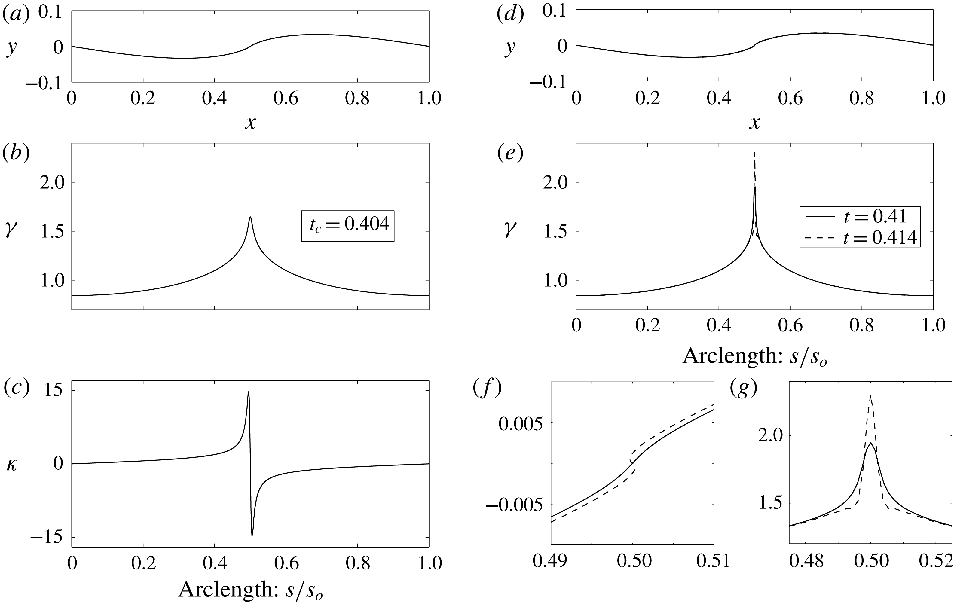
Figure 9(a–c) respectively shows the sheet shape as a function of the horizontal position
 $x$
, the sheet strength and curvature as functions of arclength
 $s$
, each at the critical time
 $t_{c}=0.404$
for the case with
 $N=400$
. As expected, the slope of the sheet is finite and does not display visual signs of roll-up, the sheet strength clearly forms a cusp and the curvature jump, while computed as finite, is rapidly increasing; recall figure 8(b). Figure 9(d,e) shows the sheet shape and vortex sheet strength at two times shortly after
 $t_{c}$
at
 $t=0.41$
and
 $0.414$
. The maximum curvature at these times (not shown) is
 $\unicode[STIX]{x1D705}_{max}=73$
and 2193, clearly indicating the singularity. The cusp in
 $\unicode[STIX]{x1D6FE}$
has also sharpened and increased considerably. This is a consequence of (2.11), which expresses the vorticity transport. Assuming a separation of variables solution for
 $\unicode[STIX]{x1D6FE}(s,t)$
and that
 $u_{s}$
is locally uniform in
 $s$
we obtain:
 $$\begin{eqnarray}\frac{\unicode[STIX]{x1D6FE}(s,t)}{\unicode[STIX]{x1D6FE}_{c}}=\text{exp}\left\{\frac{t-t_{c}}{\unicode[STIX]{x1D70F}}-\left|\frac{s-s_{c}}{u_{s}\unicode[STIX]{x1D70F}}\right|\right\}\end{eqnarray}$$
for
 $t>t_{c}$
and
 $|s-s_{c}|\ll 1$
, and where
 $\unicode[STIX]{x1D70F}^{-1}$
is the separation constant. Upon letting
 $\unicode[STIX]{x1D70F}=\unicode[STIX]{x0394}t$
we see that the delay in irregular point motion observed by Krasny (Reference Krasny1986b
) with larger time step is likely caused by a dampening of the vorticity transport toward the midpoint
 $s_{c}$
. As the disturbance amplitude grows in time to
 $t\approx t_{c}$
, the rotating motion of the sheet portends roll-up around
 $s_{c}$
meaning that
 $u_{s}\ll 1$
. Hence, when
 $t=t_{c}$
the form in (5.4) provides a fair approximation of the cusp in
 $\unicode[STIX]{x1D6FE}$
. We can then expect that the continual transport of vorticity toward
 $s_{c}$
will cause an exponential growth, or at any rate a rapid growth, in
 $\unicode[STIX]{x1D6FE}(s_{c},t)$
for
 $t_{c}>t$
. This could explain the conclusion of Higdon & Pozrikidis (Reference Higdon and Pozrikidis1985) that the sheet strength
 $\unicode[STIX]{x1D6FE}$
is infinite at
 $t=t_{c}$
in addition to the curvature as well as why they over predicted the critical time reported by Meiron et al. (Reference Meiron, Baker and Orszag1982).
The close-up views of the cusp in
 $\unicode[STIX]{x1D6FE}$
for
 $t>t_{c}$
plotted in figure 9(g) provide numerical evidence for this sudden large temporal growth of sheet strength at
 $s_{c}$
. Moreover, the close-up views of the corresponding sheet shapes in figure 9(f) show the concomitant initiation of the roll-up process. Previous studies have provided convincing evidence that the cusp in
 $\unicode[STIX]{x1D6FE}$
is finite at the critical time. The present work agrees with this conclusion and also adds the further result from (5.4) that the cusp value grows exponentially beyond the critical time. The double-branched spiral with
 $\unicode[STIX]{x1D6FE}$
being infinite for
 $t>t_{c}$
is obtained from (5.4) by
 $\unicode[STIX]{x1D70F}\rightarrow 0$
, which would correspond to an instantaneous orbital period of a particle at the point
 $s_{c}$
. Either way, the large growth of
 $\unicode[STIX]{x1D6FE}$
for
 $t>t_{c}$
is clearly the driving force behind the roll-up, which will cause the rapid formation of turns in the spiral. Unfortunately, shortly after the critical time the current computation succumbs to errors associated with the attempt, but inevitable inability of the spline to represent the infinite curvature and number of turns that would develop within the spiral core.
6 Concluding remarks
This study re-examined the problem of two-dimensional inviscid vortex sheet roll-up via a method that maintains the sheet as a segmented, but connected object. In this way, the effect of sheet curvature is explicitly included. Additionally, a model for the velocity that a sheet segment induces upon itself is derived based on the physical requirement that this velocity remain finite. This is achieved by a particular form of the local vortex sheet strength that allows direct integration through the singularity of the Birkhoff–Rott equation and results in a uniform self-induced velocity normal to the segment. It was shown that the self-induced velocity method of Fink & Soh (Reference Fink and Soh1978) corresponds to a special case of the present one in which the sheet strength is approximated by the leading-order term of its Taylor series expansion. The significant advantage of the current method is the freedom to rediscretize the segment endpoints to any desired spacing. The self-induced velocity corresponds to the local contribution of the Cauchy principle value integral and ensures that the coincident endpoints of two sheet segments remain connected. As a result, nonlinear stretching of the sheet is also explicitly taken into account and represents the transport of vorticity within the sheet.
The method was applied to two classic problems. The first was a finite vortex sheet with an elliptical circulation distribution. It was found that the self-induced velocity is critical in initiating the roll-up process and is significant in regions where the curvature and/or the gradient of the sheet strength are large. These effects stretch the sheet such that the turns within the rolled-up spiral are slightly widened by the outwardly radial self-induced velocity. When the continuous representation of the sheet explicitly includes the tip, the infinite strength density there naturally concentrates a portion of circulation at the tip and around which many tightly wound turns appear. However, there is still a ‘void’ in the middle of the spiral where the infinite number of turns within the inner core cannot be resolved. In an attempt to capture more turns and reduce the size of the void, the tip of the sheet was treated as an isolated point vortex akin to the similarity calculations of Pullin (Reference Pullin1978). The vortex accumulates circulation based on the conservation of impulse for a small finite amount of time. This corresponds to the circulation contained within the asymptotic inviscid spiral that immediately forms, but cannot be fully resolved.
The second problem was the Kelvin–Helmholtz instability of a periodically perturbed infinite vortex sheet. Here, the ability to rediscretize the segment endpoints of the sheet to equal spacing of circulation was used and found to be important for the accurate motion of the sheet. The specific initial condition studied by Krasny (Reference Krasny1986b
) was investigated. However, the critical time
 $t_{c}$
of the sheet was instead predicted based on the formation of a cusp in the vortex sheet strength
 $\unicode[STIX]{x1D6FE}$
at the midpoint where roll-up will occur. For small disturbance amplitudes,
 $\unicode[STIX]{x1D716}$
, the predicted critical times were truer to the asymptotic relation for
 $\unicode[STIX]{x1D716}\ll 1$
than the point vortex method, whereas for larger
 $\unicode[STIX]{x1D716}$
the critical times were lower. These features were interpreted as due to the sheet representation such that the nonlinear stretching/excitation of the initial disturbance is dampened/amplified (Moore Reference Moore1979) for small/larger amplitudes. The cusp value of the vortex sheet strength at
 $t_{c}$
was also computed and showed that the larger the initial amplitude, the more vorticity that is transported to location of the singularity formation, which results in smaller critical times. Numerical evidence that the cusp value in
 $\unicode[STIX]{x1D6FE}$
is finite complements that of previous claims. However, a simplifying assumption applied to the vorticity transport equation results in the prediction that for
 $t>t_{c}$
the cusp value increases rapidly in time. This was also numerically supported by the computations, which showed a large local increase in
 $\unicode[STIX]{x1D6FE}$
that leads to the initial stage of roll-up. Unfortunately, calculation of the roll-up for large times past
 $t_{c}$
was not possible owing to presence of the singularity forming in the middle of the sheet as opposed to the tip.
The effects of curvature, the self-induced velocity and their role in representing vorticity transport are important features of the method presented in this paper. There is anecdotal evidence that the stability of the calculations for evolving the governing singular integral equation is improved, although this has not been rigorously proved. Conventional point vortex methods do not include these effects explicitly and are notoriously susceptible to irregular motion. However, the simple implementation of these methods makes them attractive. In particular, the vortex blob method can yield an accurate approximation of the sheet evolution while providing stability and capturing small-scale features where the current method has failed to do so. However, considering the blob method as a regularizing kernel it could be straightforwardly implemented into our method. While this option was not presently explored, it makes an ideal topic for future work.
Acknowledgements
The author’s acknowledge the partial support of the AFOSR and the ONR in this work. We also sincerely appreciate the comments of the referees, which helped improved the quality, breadth and impact of this paper.