2.1 Proper orthogonal decomposition of a discrete system

POD extracts a set of spatial modes based on the energy of the flow structures. For a discrete system, studied either experimentally or by numerical simulations, the flow quantity $v$ of a certain temporal instantaneous (e.g. the $i$ th) flow field can be written as a column vector,

(2.1) $$\begin{eqnarray}\displaystyle \boldsymbol{v}_{i}=[v_{1i},v_{2i},\ldots ,v_{ji},\ldots ,v_{Mi}]^{\text{T}}, & & \displaystyle\end{eqnarray}$$

where the components $v_{ji}$ are the values of the quantity at the spatial point $j$ at temporal instant $i$ , and $M$ is the total number of spatial points in the experiment or numerical simulation. The superscript T represents the transpose of the vector or matrix. With a set of data samples at different temporal instants with a constant time interval, the data samples can be written as a matrix,

(2.2) $$\begin{eqnarray}\displaystyle \unicode[STIX]{x1D651}_{N}=[\boldsymbol{v}_{1},\boldsymbol{v}_{2},\ldots ,\boldsymbol{v}_{N}], & & \displaystyle\end{eqnarray}$$

where $N$ is the number of temporal data samples, or columns in matrix $\unicode[STIX]{x1D651}_{N}$ . Usually, the dimension of the matrix $M\gg N$ for fluid flow problems. We define the energy matrix $\unicode[STIX]{x1D64D}$ as

(2.3) $$\begin{eqnarray}\displaystyle \unicode[STIX]{x1D64D}=\frac{1}{N}\unicode[STIX]{x1D651}_{N}\unicode[STIX]{x1D651}_{N}^{\text{T}}, & & \displaystyle\end{eqnarray}$$

which is a symmetrical and semi-positive-definite matrix, whose eigenvalues can be obtained by

(2.4) $$\begin{eqnarray}\displaystyle & \displaystyle \unicode[STIX]{x1D64D}\boldsymbol{U}=\boldsymbol{U}\unicode[STIX]{x1D72E}^{\prime }, & \displaystyle\end{eqnarray}$$

(2.5) $$\begin{eqnarray}\displaystyle & \displaystyle \boldsymbol{U}=[\boldsymbol{u}_{\mathbf{1}},\boldsymbol{u}_{\mathbf{2}},\ldots ,\boldsymbol{u}_{N}], & \displaystyle\end{eqnarray}$$

(2.6) $$\begin{eqnarray}\displaystyle & \displaystyle \unicode[STIX]{x1D72E}^{\prime }=\text{diag}(\unicode[STIX]{x1D70E}_{1}^{\prime },\unicode[STIX]{x1D70E}_{2}^{\prime },\ldots ,\unicode[STIX]{x1D70E}_{N}^{\prime }). & \displaystyle\end{eqnarray}$$

Here the column vectors $\boldsymbol{u}_{i}$ of the matrix $\unicode[STIX]{x1D650}$ are the eigenvectors of $\unicode[STIX]{x1D64D}$ , referred to as POD modes, and $\unicode[STIX]{x1D70E}_{i}^{\prime }$ in the diagonal matrix $\unicode[STIX]{x1D72E}^{\prime }$ is the eigenvalue, identical to the energy of $\boldsymbol{u}_{i}$ . The POD method is equivalent to the singular value decomposition (SVD) of matrix $\unicode[STIX]{x1D651}_{N}$ in such a way that

(2.7) $$\begin{eqnarray}\displaystyle \unicode[STIX]{x1D651}_{N}=\unicode[STIX]{x1D650}\unicode[STIX]{x1D72E}\unicode[STIX]{x1D651}^{\text{H}}, & & \displaystyle\end{eqnarray}$$

where $\unicode[STIX]{x1D72E}=\sqrt{N\unicode[STIX]{x1D72E}^{\prime }}$ is a diagonal matrix of rank $n$ (usually $n=N$ ) with non-zero singular values $\{\unicode[STIX]{x1D70E}_{1},\ldots ,\unicode[STIX]{x1D70E}_{n}\}$ on its main diagonal, and $\unicode[STIX]{x1D650}$ and $\unicode[STIX]{x1D651}$ are matrices with unit and orthogonal columns, i.e.

(2.8a,b ) $$\begin{eqnarray}\displaystyle \unicode[STIX]{x1D650}\in \mathbb{C}^{N\times n},\quad \unicode[STIX]{x1D650}^{\text{H}}\unicode[STIX]{x1D650}=\unicode[STIX]{x1D644}, & & \displaystyle\end{eqnarray}$$

(2.9a,b ) $$\begin{eqnarray}\displaystyle \unicode[STIX]{x1D651}\in \mathbb{C}^{n\times M},\quad \unicode[STIX]{x1D651}^{\text{H}}\unicode[STIX]{x1D651}=\unicode[STIX]{x1D644}, & & \displaystyle\end{eqnarray}$$

where the superscript H refers to the Hermitian transpose of the matrix.

2.2 Dynamic mode decomposition

The DMD method needs one more temporal realisation of the flow field than POD, and the data samples can be written as two matrices:

(2.10a,b ) $$\begin{eqnarray}\displaystyle \unicode[STIX]{x1D651}_{N1}=[\boldsymbol{v}_{0},\boldsymbol{v}_{1},\ldots ,\boldsymbol{v}_{N-1}],\quad \unicode[STIX]{x1D651}_{N2}=[\boldsymbol{v}_{1},\boldsymbol{v}_{2},\ldots ,\boldsymbol{v}_{N}]. & & \displaystyle\end{eqnarray}$$

It is assumed that the constant time interval $\unicode[STIX]{x0394}t$ is small enough that the two matrices can be related by a linear mapping, i.e.

(2.11) $$\begin{eqnarray}\displaystyle \unicode[STIX]{x1D651}_{N2}=\unicode[STIX]{x1D63C}\unicode[STIX]{x1D651}_{N1}, & & \displaystyle\end{eqnarray}$$

where $\unicode[STIX]{x1D63C}$ is the evolving matrix of the dynamical system. Matrix $\unicode[STIX]{x1D63C}$ is unknown and can be seriously ill-conditioned if obtained by taking the pseudo-inverse of $\unicode[STIX]{x1D651}_{N1}$ ; thus an orthogonal decomposition of $\unicode[STIX]{x1D651}_{N1}$ is needed to solve the eigenvalue problem correctly. Performing SVD on $\unicode[STIX]{x1D651}_{N1}$ as shown in (2.7), the linear mapping shown in (2.11) can further be expressed as

(2.12) $$\begin{eqnarray}\displaystyle \unicode[STIX]{x1D651}_{N2}=\unicode[STIX]{x1D63C}\unicode[STIX]{x1D650}\unicode[STIX]{x1D72E}\unicode[STIX]{x1D651}^{\text{H}}. & & \displaystyle\end{eqnarray}$$

Then the projection of $\unicode[STIX]{x1D63C}$ on the basis $\unicode[STIX]{x1D650}$ can be expressed as

(2.13) $$\begin{eqnarray}\displaystyle \unicode[STIX]{x1D63C}^{\prime }=\unicode[STIX]{x1D650}^{\text{H}}\unicode[STIX]{x1D63C}\unicode[STIX]{x1D650}=\unicode[STIX]{x1D650}^{\text{H}}\unicode[STIX]{x1D651}_{N2}\unicode[STIX]{x1D651}\unicode[STIX]{x1D72E}^{-1}. & & \displaystyle\end{eqnarray}$$

Note that $\unicode[STIX]{x1D63C}^{\prime }$ shares the same eigenvalues as $\unicode[STIX]{x1D63C}$ , but its rank is much lower. The eigenvalues $\unicode[STIX]{x1D707}_{i}~(i=1,2,\ldots ,n)$ and eigenvectors $\boldsymbol{w}_{i}$ of $\unicode[STIX]{x1D63C}^{\prime }$ are obtained by solving the following eigenvalue problem:

(2.14) $$\begin{eqnarray}\displaystyle & \displaystyle \unicode[STIX]{x1D63C}^{\prime }\boldsymbol{W}=\boldsymbol{W}\unicode[STIX]{x1D726}, & \displaystyle\end{eqnarray}$$

(2.15) $$\begin{eqnarray}\displaystyle & \displaystyle \unicode[STIX]{x1D726}=\text{diag}(\unicode[STIX]{x1D707}_{1},\unicode[STIX]{x1D707}_{2},\ldots ,\unicode[STIX]{x1D707}_{n}), & \displaystyle\end{eqnarray}$$

(2.16) $$\begin{eqnarray}\displaystyle & \displaystyle \boldsymbol{W}=[\boldsymbol{w}_{1},\boldsymbol{w}_{2},\ldots ,\boldsymbol{w}_{n}], & \displaystyle\end{eqnarray}$$

and the eigenmodes are obtained by

(2.17) $$\begin{eqnarray}\displaystyle \unicode[STIX]{x1D731}=\unicode[STIX]{x1D650}\boldsymbol{W}. & & \displaystyle\end{eqnarray}$$

2.3 Data-driven reduced-order model construction

The present data-driven ROM construction method uses POD modes as the orthogonal basis and DMD eigenvalues to represent the temporal evolution of the modes. With the POD modes obtained in (2.4), each temporal realisation of the flow field can be expressed as a linear combination of the POD modes,

(2.18a,b ) $$\begin{eqnarray}\displaystyle \boldsymbol{v}_{0}=\mathop{\sum }_{i=1}^{N}b_{i}(0)\boldsymbol{u}_{i},\quad \boldsymbol{v}_{1}=\mathop{\sum }_{i=1}^{N}b_{i}(\unicode[STIX]{x0394}t)\boldsymbol{u}_{i},\ldots ,\quad \boldsymbol{v}_{N}=\mathop{\sum }_{i=1}^{N}b_{i}(N\unicode[STIX]{x0394}t)\boldsymbol{u}_{i}.\qquad & & \displaystyle\end{eqnarray}$$

Substituting the above linear expansions into the linear mapping (2.11), we get

(2.19) $$\begin{eqnarray}\displaystyle \unicode[STIX]{x1D650}\unicode[STIX]{x1D63D}_{2}=\unicode[STIX]{x1D63C}\unicode[STIX]{x1D650}\unicode[STIX]{x1D63D}_{1}, & & \displaystyle\end{eqnarray}$$

where $\unicode[STIX]{x1D63D}_{1}$ and $\unicode[STIX]{x1D63D}_{2}$ are the matrices of the temporally evolving coefficients:

(2.20) $$\begin{eqnarray}\displaystyle & \displaystyle \unicode[STIX]{x1D63D}_{1}=\left[\begin{array}{@{}cccc@{}}b_{1}(0) & b_{1}(\unicode[STIX]{x0394}t) & \cdots \, & b_{1}((N-1)\unicode[STIX]{x0394}t)\\ b_{2}(0) & b_{2}(\unicode[STIX]{x0394}t) & \cdots \, & b_{2}((N-1)\unicode[STIX]{x0394}t)\\ \vdots & \vdots & \ddots & \vdots \\ b_{N}(0) & b_{N}(\unicode[STIX]{x0394}t) & \cdots \, & b_{N}((N-1)\unicode[STIX]{x0394}t)\end{array}\right], & \displaystyle\end{eqnarray}$$

(2.21) $$\begin{eqnarray}\displaystyle & \displaystyle \unicode[STIX]{x1D63D}_{2}=\left[\begin{array}{@{}cccc@{}}b_{1}(\unicode[STIX]{x0394}t) & b_{1}(2\unicode[STIX]{x0394}t) & \cdots \, & b_{1}(N\unicode[STIX]{x0394}t)\\ b_{2}(\unicode[STIX]{x0394}t) & b_{2}(2\unicode[STIX]{x0394}t) & \cdots \, & b_{2}(N\unicode[STIX]{x0394}t)\\ \vdots & \vdots & \ddots & \vdots \\ b_{N}(\unicode[STIX]{x0394}t) & b_{N}(2\unicode[STIX]{x0394}t) & \cdots \, & b_{N}(N\unicode[STIX]{x0394}t)\end{array}\right]. & \displaystyle\end{eqnarray}$$

Equation (2.19) can be further written as

(2.22) $$\begin{eqnarray}\displaystyle \unicode[STIX]{x1D63D}_{2}=\unicode[STIX]{x1D650}^{\text{H}}\unicode[STIX]{x1D63C}\unicode[STIX]{x1D650}\unicode[STIX]{x1D63D}_{1}=\unicode[STIX]{x1D63C}^{\prime }\unicode[STIX]{x1D63D}_{1}. & & \displaystyle\end{eqnarray}$$

Note that the SVD is used in both methods, as shown in (2.5) and (2.8). Equation (2.22) indicates that the temporally evolving matrix $\unicode[STIX]{x1D63C}^{\prime }$ is the same as the matrix defined in (2.13) for DMD, which is the projection of the temporally evolving matrix $\unicode[STIX]{x1D63C}$ on the orthogonal basis $\unicode[STIX]{x1D650}$ . In this sense, the POD and DMD modes are equivalent, as the latter are simply linear combinations of the former. The temporal evolution of the POD modes can be obtained via the DMD eigenvalues and eigenvectors in (2.14). As stated in the previous section, the essential step of the POD–Galerkin method is to obtain the matrix of temporal coefficients. However, the projection of the equations is quite complicated, and is restricted by many factors, including the numerical schemes and boundary conditions. The present data-driven method avoids all of these problems, and the matrix of temporal coefficients can be easily obtained from data samples.

The discrete form of the temporal evolution equation can be expressed as follows:

(2.23) $$\begin{eqnarray}\displaystyle \boldsymbol{b}(t+\unicode[STIX]{x0394}t)=\unicode[STIX]{x1D63C}^{\prime }\boldsymbol{b}(t), & & \displaystyle\end{eqnarray}$$

where

(2.24) $$\begin{eqnarray}\displaystyle & \displaystyle \boldsymbol{b}(t+\unicode[STIX]{x0394}t)=[b_{1}(t+\unicode[STIX]{x0394}t),b_{2}(t+\unicode[STIX]{x0394}t),\ldots ,b_{N}(t+\unicode[STIX]{x0394}t)]^{\text{T}}, & \displaystyle\end{eqnarray}$$

(2.25) $$\begin{eqnarray}\displaystyle & \displaystyle \boldsymbol{b}(t)=[b_{1}(t),b_{2}(t),\ldots ,b_{N}(t)]^{\text{T}}. & \displaystyle\end{eqnarray}$$

With a group of initial values, the temporal coefficients can be obtained via the above linear mapping. If desired, the formula can be further expressed as ODEs, enabling continuous temporal coefficients to be obtained. The eigenvalues and eigenvectors of $\unicode[STIX]{x1D63C}^{\prime }$ can be calculated by (2.14), and the logarithms of the eigenvalues

(2.26) $$\begin{eqnarray}\displaystyle \unicode[STIX]{x1D729}=\text{diag}(\ln \unicode[STIX]{x1D707}_{1},\ln \unicode[STIX]{x1D707}_{2},\ldots ,\ln \unicode[STIX]{x1D707}_{n})/\unicode[STIX]{x0394}t & & \displaystyle\end{eqnarray}$$

are the eigenvalues of the ODEs, representing the frequency and amplification rate of the DMD modes. Therefore,

(2.27) $$\begin{eqnarray}\displaystyle \unicode[STIX]{x1D63C}_{c}=\boldsymbol{W}^{-1}\unicode[STIX]{x1D729}\boldsymbol{W} & & \displaystyle\end{eqnarray}$$

is the temporal evolution matrix of the ODEs, i.e.

(2.28) $$\begin{eqnarray}\displaystyle \frac{\text{d}\boldsymbol{b}(t)}{\text{d}t}=\unicode[STIX]{x1D63C}_{c}\boldsymbol{b}(t), & & \displaystyle\end{eqnarray}$$

which can be solved by classical algorithms such as the Runge–Kutta method.

Because the number of temporal data samples is usually of the order of $O(10^{2})$ , the dimensionality of the ROM is still high. The sparsity-promoting (SP) dynamic mode decomposition (SPDMD) (Jovanović et al. Reference Jovanović, Schmid and Nichols2014) provides a way to lower its dimensionality. SPDMD addresses the dimension reduction of the full-rank decomposition by adding a penalty function term in the standard optimisation problem. The SP method removes the modes with large damping rates or small amplitudes and leaves only those with strong contributions to the original data sequence. In temporal equilibrium systems, there are no significant damping modes, and the SP method only removes modes with small amplitudes, leaving the important modes needed to construct an appropriate ROM. Because the POD modes are ranked by energy, the dimensionality of the ROM should be larger than, or at least equal to, the number of modes selected by the SP method. Therefore, the truncation of $\unicode[STIX]{x1D63C}^{\prime }$ can be performed as follows. Assuming that the appropriate number of ROM dimensions is $r$ , and the $r$ POD modes are used and written as $\unicode[STIX]{x1D650}_{r}\in \mathbb{R}^{M\times r}$ , then we have

(2.29) $$\begin{eqnarray}\displaystyle \unicode[STIX]{x1D63C}_{r}=\unicode[STIX]{x1D650}_{r}^{\text{H}}\unicode[STIX]{x1D63C}\unicode[STIX]{x1D650}_{r}=\unicode[STIX]{x1D650}_{r}^{\text{H}}\unicode[STIX]{x1D651}_{N2}\unicode[STIX]{x1D651}_{r}\unicode[STIX]{x1D72E}_{r}^{-1}, & & \displaystyle\end{eqnarray}$$

where the matrix with subscript $r$ on the right-hand side represents the truncated matrix, leaving the first $r$ rows (for $\unicode[STIX]{x1D650}^{\text{H}}$ ), columns (for $\unicode[STIX]{x1D651}$ ) or both (for $\unicode[STIX]{x1D72E}$ ). Substituting the matrix $\unicode[STIX]{x1D63C}_{r}$ into (2.28) and using only the first $r$ temporal coefficients $b_{1},b_{2},\ldots ,b_{r}$ , then an $r$ -dimensional ROM can be obtained.

The ROM construction process is briefly summarised as follows:

1. (1) Write the data samples (with a constant time interval) obtained by numerical simulations or experimental measurements in the form of matrices $\unicode[STIX]{x1D651}_{N1}$ and $\unicode[STIX]{x1D651}_{N2}$ as dictated by (2.10).

2. (2) Perform SVD via equation (2.7) on the matrix $\unicode[STIX]{x1D651}_{N1}$ to obtain the orthogonal basis $\unicode[STIX]{x1D650}$ and the singular values $\unicode[STIX]{x1D72E}$ . The energy of each mode is obtained.

3. (3) Perform DMD by solving (2.11)–(2.14) and (2.26).

4. (4) Truncate $\unicode[STIX]{x1D63C}^{\prime }$ to lower dimensions according to the SPDMD results or the energy of the POD modes according to (2.29), and obtain the temporal evolution matrix from (2.27) by replacing $\unicode[STIX]{x1D63C}_{c}$ with $\unicode[STIX]{x1D63C}_{r}$ .

5. (5) Solve (2.28) numerically to give the temporal evolution of the POD modes.

3.1 Numerical set-up

The supersonic boundary layer transition for an ideal gas and a Newtonian fluid is simulated by DNS using OPENCFD-1.10.4, developed by Li et al. (Reference Li, Fu, Ma and Liang2010). The conservative governing equations are solved numerically with the high-order finite difference method. The convection terms are approximated with the seventh-order weighted essentially non-oscillatory (WENO) scheme, and the viscous terms are approximated with the sixth-order central difference scheme. The third-order total variation diminishing (TVD) Runge–Kutta scheme is adopted for time advancement. The details of the numerical schemes and validation of the code can be found in Li et al. (Reference Li, Fu, Ma and Liang2010).

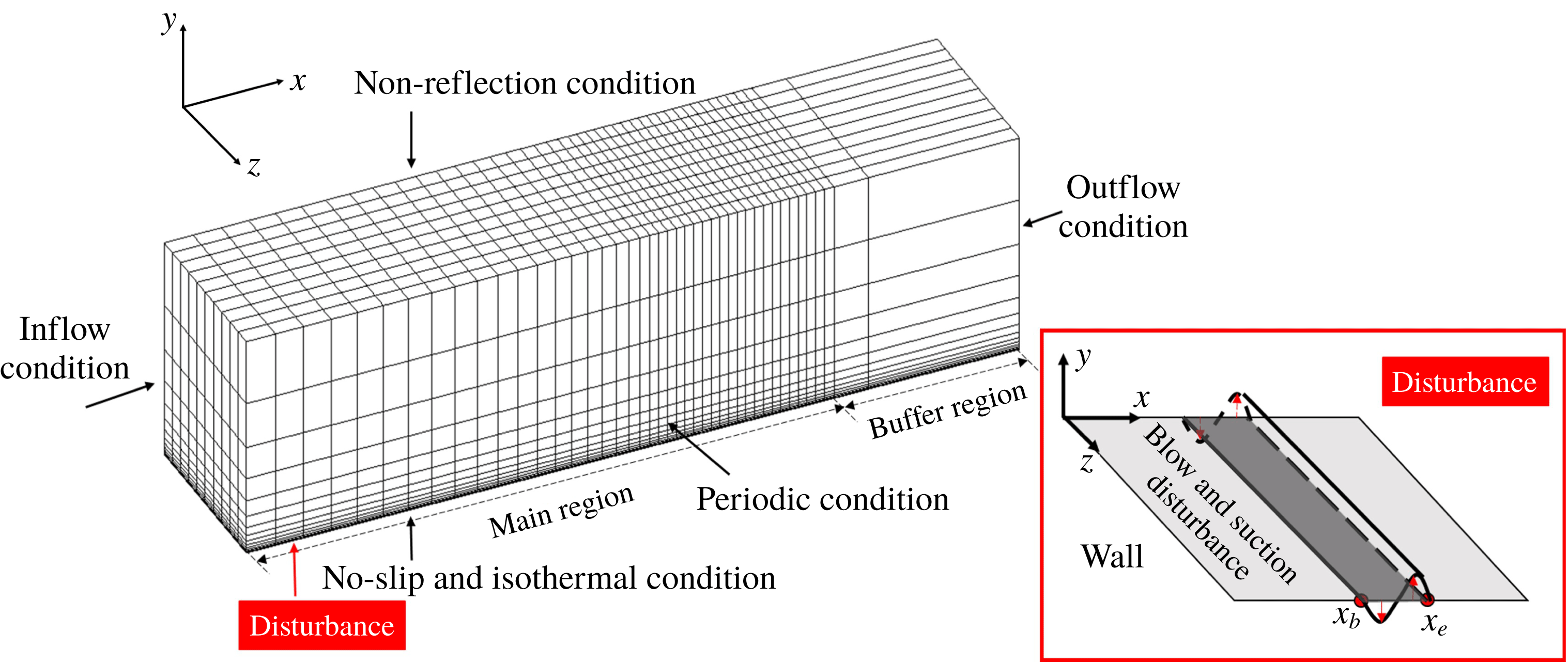
The computational configurations and boundary conditions are shown in figure 1. The computational domain is divided into the main region with a fine mesh and the buffer region with gradually coarser meshes to minimise the influence of the outlet boundary condition. At the inlet of the computational domain, the laminar profiles of density ( $\unicode[STIX]{x1D70C}$ ), velocity ( $u$ , $v$ and $w$ , the velocity components in the $x$ , $y$ and $z$ directions) and temperature ( $T$ ) are set as those obtained by the two-dimensional numerical simulation with the same parameters and boundary conditions. At the wall, a no-slip condition is adopted for velocities and the isothermal condition for temperature. A non-reflection condition is adopted at the upper boundary, and a periodic condition in the spanwise direction.

For the supersonic boundary layer, the flow parameters are set according to Pirozzoli, Grasso & Gatski (Reference Pirozzoli, Grasso and Gatski2004), i.e. the free-stream Reynolds number $Re=635\,000~\text{inch}^{-1}$ , Mach number $Ma=2.25$ and temperature 169.0 K. The wall temperature is 1.9 times the free-stream temperature. All of the flow quantities in the following are non-dimensionalised by the reference density, velocity and temperature of the free stream, and the characteristic length is chosen to be 1 inch. Two separate cases are considered, with linear and nonlinear disturbances (inducing natural and bypass transitions, respectively). The computational domain and grid numbers for each case are listed in table 1, in which the subscripts $x$ , $y$ and $z$ denote streamwise, wall-normal and spanwise directions, respectively.

Figure 2.

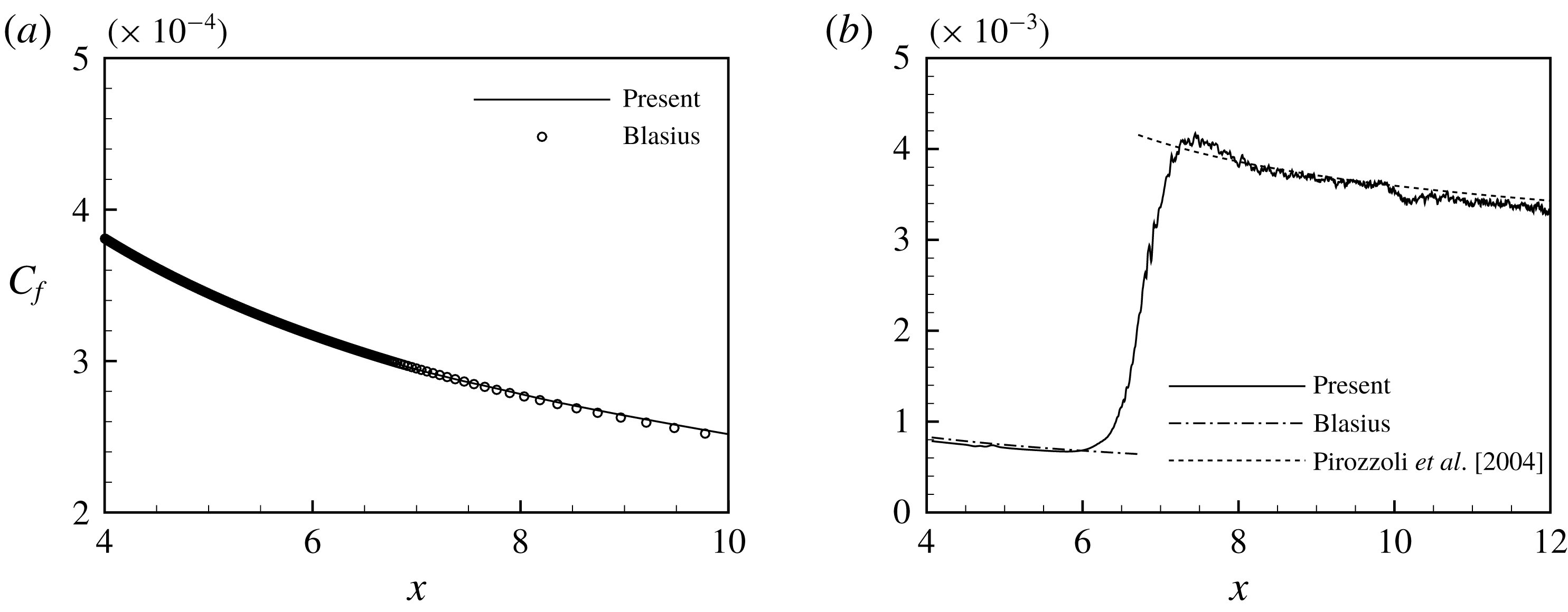
Streamwise variation of $C_{f}$ : (a) linear case, and (b) nonlinear case.

Table 1.

Computational parameters.

To trigger the transition, a periodic blowing and suction disturbance is introduced at the wall in the region of $x=4.0{-}4.5$ . The formulation of the disturbance can be found in Pirozzoli et al. (Reference Pirozzoli, Grasso and Gatski2004). The frequencies introduced are 3.982 and 7.854, with spanwise wavenumbers of 35.9 and 71.8 (corresponding to one and two waves in the spanwise direction), which are linearly unstable according to linear stability analysis. In the linear case, the disturbance amplitudes are set to 0.0003 for the two frequencies, and in the nonlinear case both are set to 0.004. The streamwise distributions of the mean skin friction coefficient ( $C_{f}$ ) are shown in figure 2 in comparison with that of the laminar Blasius boundary layer and that of a turbulent flow given by Pirozzoli et al. (Reference Pirozzoli, Grasso and Gatski2004). The $C_{f}$ values before and after the transition show good agreement with the reference results of laminar and turbulent flows, respectively.

3.2 Reduced-order model of natural transition

First, the ROM of the flow with a linear disturbance is built to validate the proposed ROM construction method. The flow quantities used in the analysis are the three velocity components $u$ , $v$ and $w$ , density $\unicode[STIX]{x1D70C}$ and temperature $T$ . The mean values are subtracted so that only the fluctuating parts are considered. The data from all of the grid points constitute the data sample at each temporal instant, and a total of 201 realisations with the time interval of $\unicode[STIX]{x0394}t=0.05$ are used to construct the ROM.

Notably, the inner product in the present POD is simply defined as

(3.1) $$\begin{eqnarray}(\boldsymbol{v}_{i},\boldsymbol{v}_{j})=\mathop{\sum }_{n=1}^{M}(u_{ni}u_{nj}+v_{ni}v_{nj}+w_{ni}w_{nj}+\unicode[STIX]{x1D70C}_{ni}\unicode[STIX]{x1D70C}_{nj}+T_{ni}T_{nj}).\end{eqnarray}$$

Therefore, the term POD ‘energy’, used for brevity in the following discussion, refers to the Euclid norm of the vector instead of the real physical energy. As pointed out in § 1, the definition of the inner product is one of the most important problems in ROM. Rowley et al. (Reference Rowley, Colonius and Murray2004) and Kalashnikova & Barone (Reference Kalashnikova and Barone2010) suggested that the inner product must satisfy the definition of total energy, to ensure that the projection of the modes on the governing equations is physically reasonable. Although the proposed data-driven method here has no need of governing equations, the results may still be dependent on the definition of the inner product. Because this paper focuses on the data-driven method itself, and this method can be used with any definition of the inner product, we will not further discuss the form of the inner product.

Following the algorithm described in § 2, the method will be explained in detail using the results of each step in ROM construction.

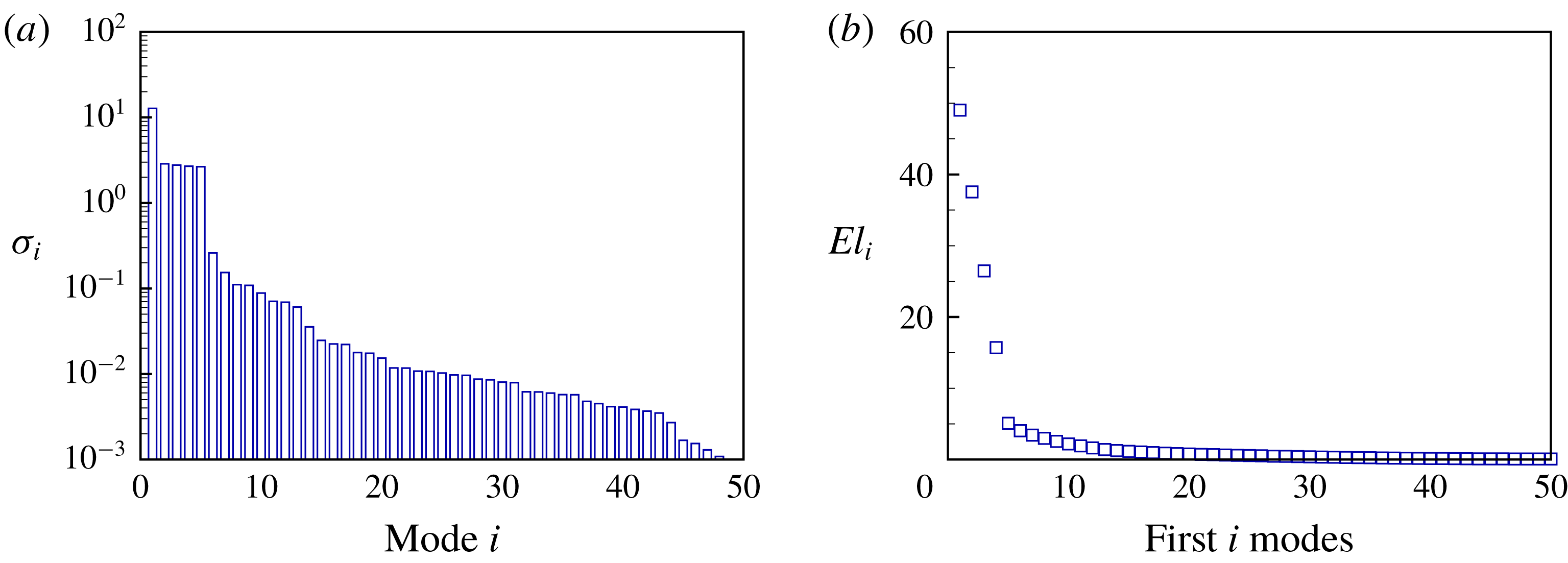
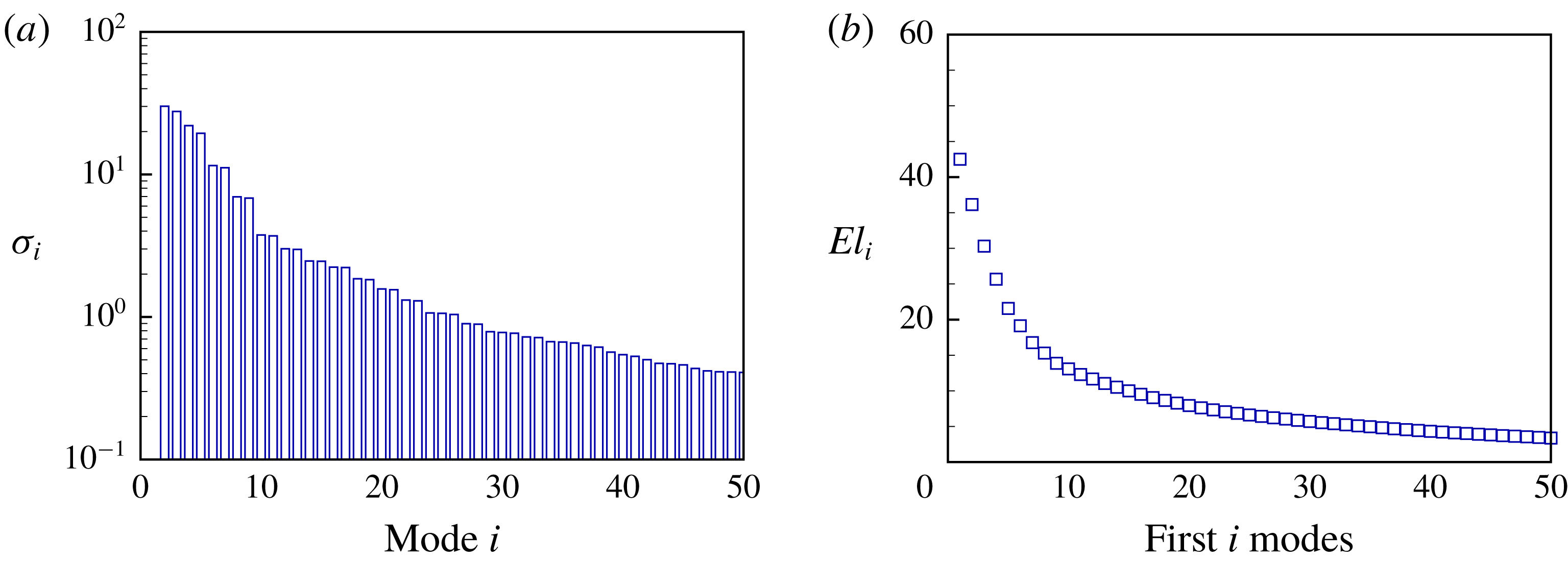
SVD is performed on the data sample matrix to obtain the POD modes and their energies, which are represented by the eigenvalues in (2.4). The total energy loss of the first $i$ modes is defined as

(3.2) $$\begin{eqnarray}El_{i}=\left(1-\mathop{\sum }_{j=1}^{i}\unicode[STIX]{x1D70E}_{j}\left/\mathop{\sum }_{j=1}^{N}\right.\unicode[STIX]{x1D70E}_{j}\right)\times 100\,\%.\end{eqnarray}$$

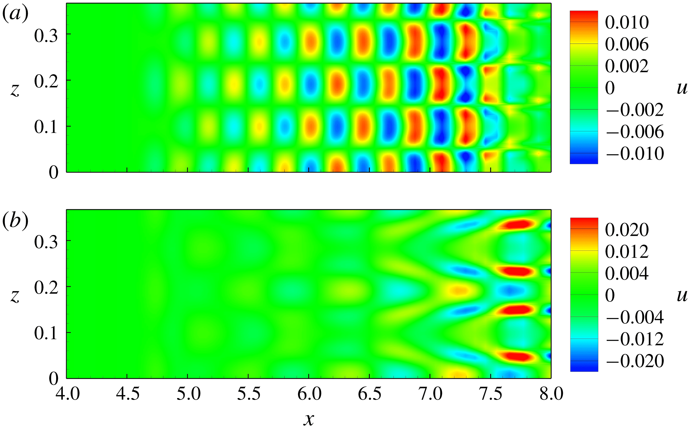
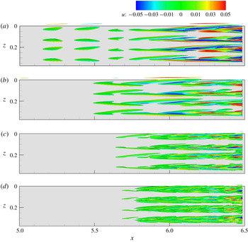
As shown in figure 3, the first five modes are much higher in energy than the others, and together account for more than 95 % of the total energy. This indicates that these modes are sufficient to construct the ROM. The distributions of the streamwise disturbance velocity $u$ of mode 2 and mode 4 on the plane at $y=0.01$ are shown in figure 4. Mode 2 is clearly an H-type disturbance, while mode 4 is a K-type disturbance (Sayadi et al. Reference Sayadi, Schmid, Nichols and Moin2014).

Figure 3.

Energy of POD modes (a) and total energy loss of the first $i$ modes (b).

Figure 4.

Contours of $u$ of mode 2 (a) and mode 4 (b) on plane at $y=0.01$ .

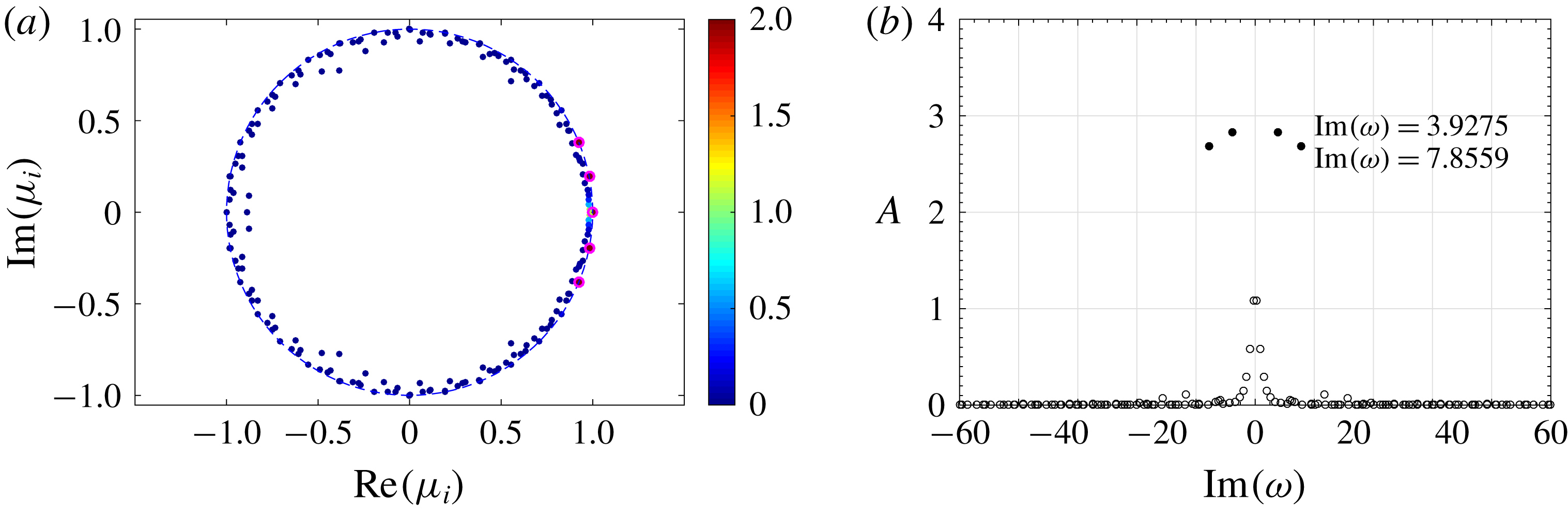
Next, DMD is applied. In figure 5(a), the eigenvalues of matrix $\unicode[STIX]{x1D63C}^{\prime }$ are shown, coloured by the initial amplitudes of the modes. The SP algorithm is performed to obtain the important modes, marked with magenta circles. All of the eigenvalues lie either on or inside the unit circle, indicating that all of the modes are either neutrally stable or decay with time. The DMD frequency spectrum is shown in figure 5(b). The selected modes are shown with solid circles, and the corresponding frequencies are 3.9275 and 7.8559, which are the same as those of the disturbance introduced at the wall. The non-oscillating mode with the highest energy is not shown in figure 5(b) because it corresponds to the average flow field. The amplitudes of the selected modes are much higher than the others.

Figure 5.

DMD eigenvalues (a) and spectrum (b); magenta circles in (a) and solid circles in (b) are modes selected by SP algorithm.

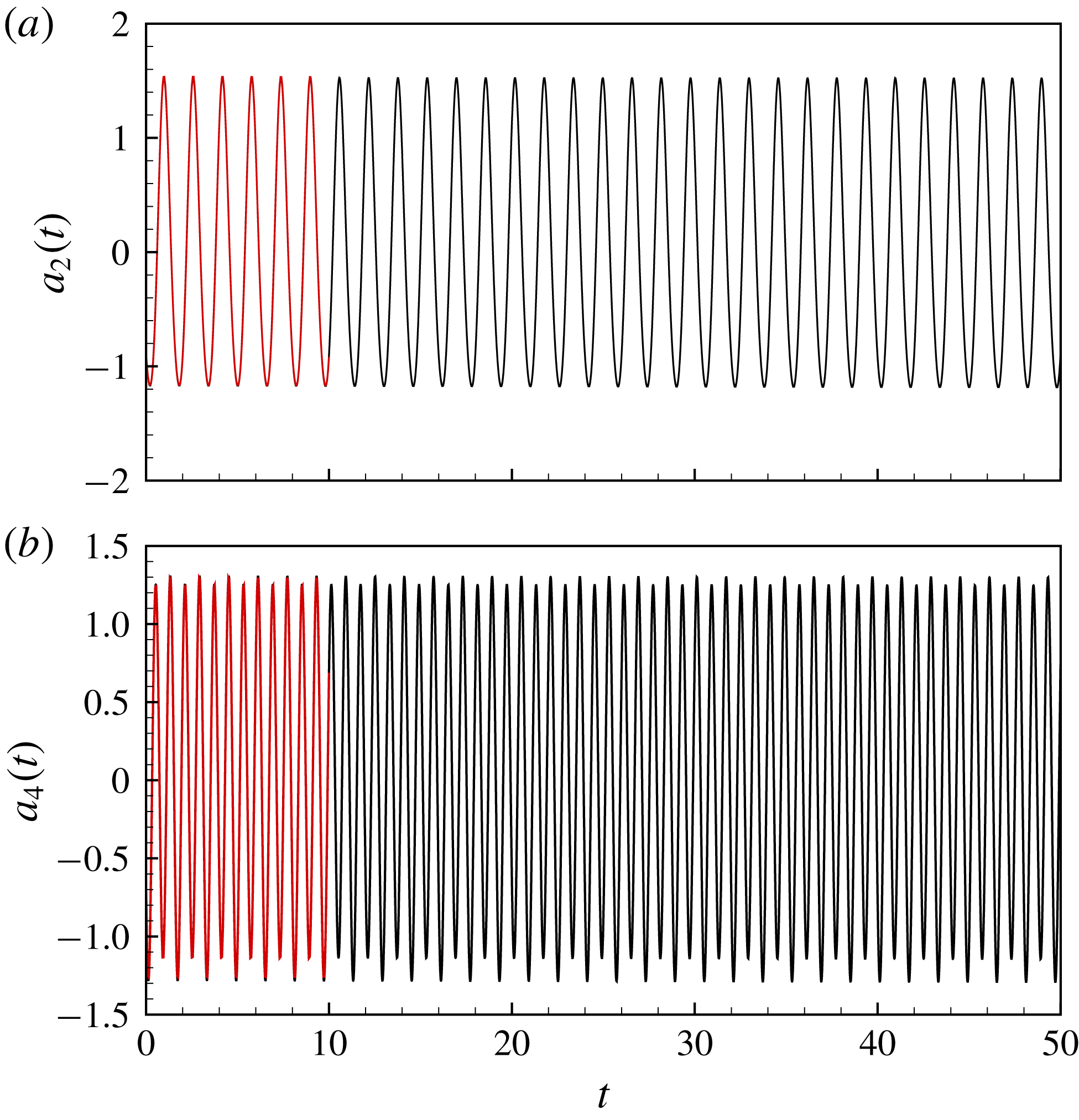
With the POD and DMD results above, the evolution matrix for the temporal coefficients of the POD modes can be easily obtained. The ODEs for the temporal evolution are solved with the fourth-order Runge–Kutta algorithm. The original DNS data are projected on the POD modes to obtain the initial values and the temporal coefficients of each mode for comparison. Because the oscillating POD modes come in pairs with different initial phases, only mode 2 and mode 4 are shown in figure 6. The temporal coefficients predicted by the ODEs agree very well with the projected DNS data within the time range used in POD. Because these modes are temporally stable and periodically evolving, the long-term evolution of the temporal coefficients should also be so. Therefore, the ROM accurately predicts the temporal evolution of the POD modes.

Figure 6.

Temporal coefficients of mode 2 (a) and mode 4 (b): red, projected DNS data; black, ROM.

3.3 Reduced-order model of bypass transition

The ability of the ROM constructed above to accurately predict the temporal evolution of the POD modes is not surprising, because the flow field analysed above is linear, and the DMD, on which the present ROM construction method is based, assumes linear mapping. The method needs to be further tested by assessing its applicability to nonlinear flows. The computational parameters for the nonlinear case are listed in table 1. Compared with the linear case, the domain is longer streamwise and finer grids are used, to ensure that the entire transitional process can be accurately captured.

The flow quantities used in constructing the ROM are the same as those in the linear case. The time interval is $\unicode[STIX]{x0394}t=0.02$ and a total of 201 temporal samples are included. The subzone in the range of $x=5.0{-}6.5$ is selected for analysis because $x=6.5$ marks the beginning of the transition (as shown in figure 2 b), and the nonlinear effects in this region are obvious.

The energy of the POD modes and the total energy loss of the first $i$ modes are shown in figure 7. The energy decreases slowly with increasing mode number, indicating the existence of complicated flow structures in the field caused by nonlinear effects. If the ROM is to capture 90 % of the total energy, 13 modes are needed, as shown in figure 7(b).

Figure 7.

Energy of POD modes (a) and total energy loss of the first $i$ modes (b).

Figure 8.

Isosurfaces of $Q=0.0001$ coloured by $u$ : (a–d) modes 2, 4, 6 and 8, respectively.

The vortical structures of the first four POD modes with the highest energy are shown in figure 8 as the isosurfaces of $Q$ , the second invariant of the velocity gradient tensor. The structures are mainly streamwise-elongated vortices. They become stronger downstream, where the velocity disturbances around the vortices are more significant, as indicated by the contours of the streamwise disturbance velocity $u$ . With increasing mode number (decreasing mode energy), the streamwise vortices become smaller and appear further downstream.

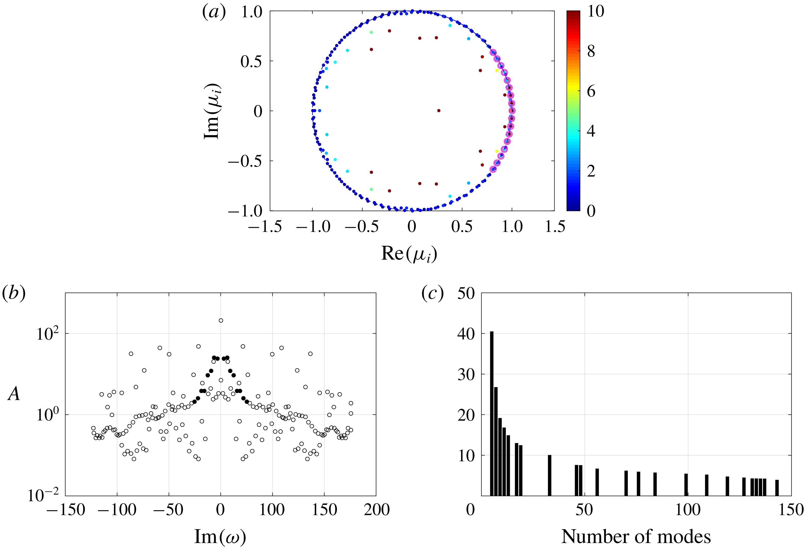
The DMD eigenvalues are shown in figure 9(a), coloured by the initial amplitude of the modes. The SP algorithm is then applied, and the modes selected are shown with magenta circles. The eigenvalues of the selected modes lie on the unit circle, indicating that the structures in these modes are neutrally stable. The DMD frequency spectrum is shown in figure 9(b), where the modes selected by the SP algorithm are shown with solid circles. The spectrum is more scattered and widely distributed as compared with the linear case. The low-frequency modes are higher in energy than the high-frequency modes. The results of the SP algorithm indicate that 19 modes are needed to capture the most important structures in the flow field. The total energy loss of the first $i$ DMD modes is also investigated. As shown in figure 9(c), 19 modes are sufficient to capture 88 % of the total energy.

Figure 9.

DMD eigenvalues (a), DMD frequency spectrum (b) and energy loss (%) as a function of the number of modes (c); magenta circles in (a) and solid circles in (b) are modes selected by SP algorithm.

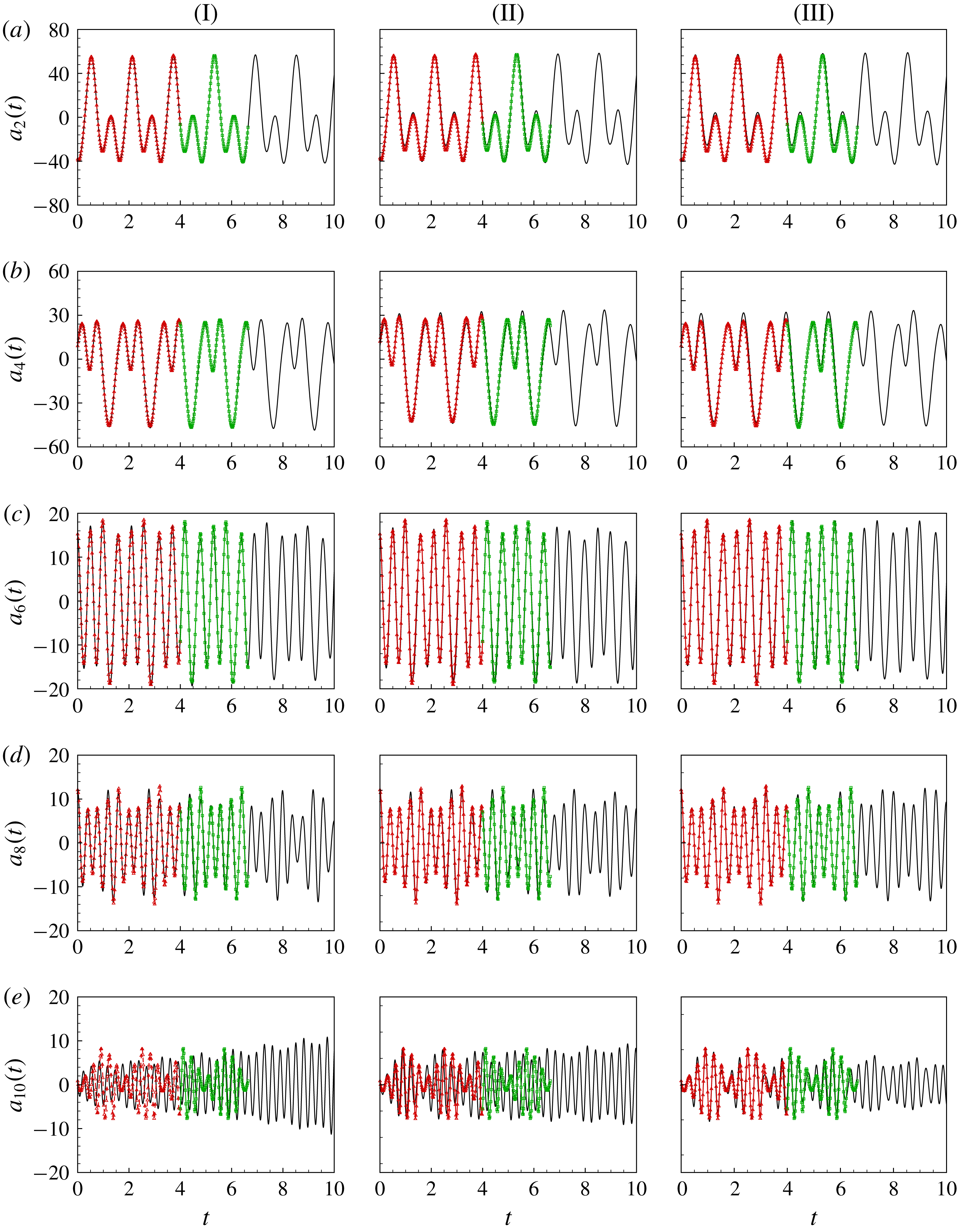
To examine the influence of the number of modes, we select 11, 15 and 21 modes, respectively, to construct the ROMs. (Note that the mode number provided by the SP algorithm is used as a reference, not a criterion, so we do not need to check whether 19 is the precise number of modes needed to establish an accurate and suitable ROM.) The temporal coefficients for each mode are obtained by solving (2.25) with the same numerical method as in the linear case. The results are compared with the projected DNS data, as shown in figure 10. The red symbols represent the projected DNS data in the time range where POD and DMD are performed (hereinafter referred to as the TRI), and the green symbols represent those beyond the TRI (hereinafter referred to as the TRO). For the temporal evolution of the lower modes 2–8, all of the ROMs yield accurate predictions both in the TRI and TRO. However, for mode 10, an obvious discrepancy can be observed between the result predicted by the ROM with 11 modes and the DNS data. Increasing the number of modes included in the ROM enhances the accuracy for mode 10, as shown by figure 10(II-e) and (III-e).

Figure 10.

Temporal coefficients of mode 2, mode 4, mode 6, mode 8 and mode 10 (a–e) given by ROMs with 11, 15 and 21 modes (I–III): — △ —, TRI; — ◻ —, TRO; ——, ROM.

Figure 11.

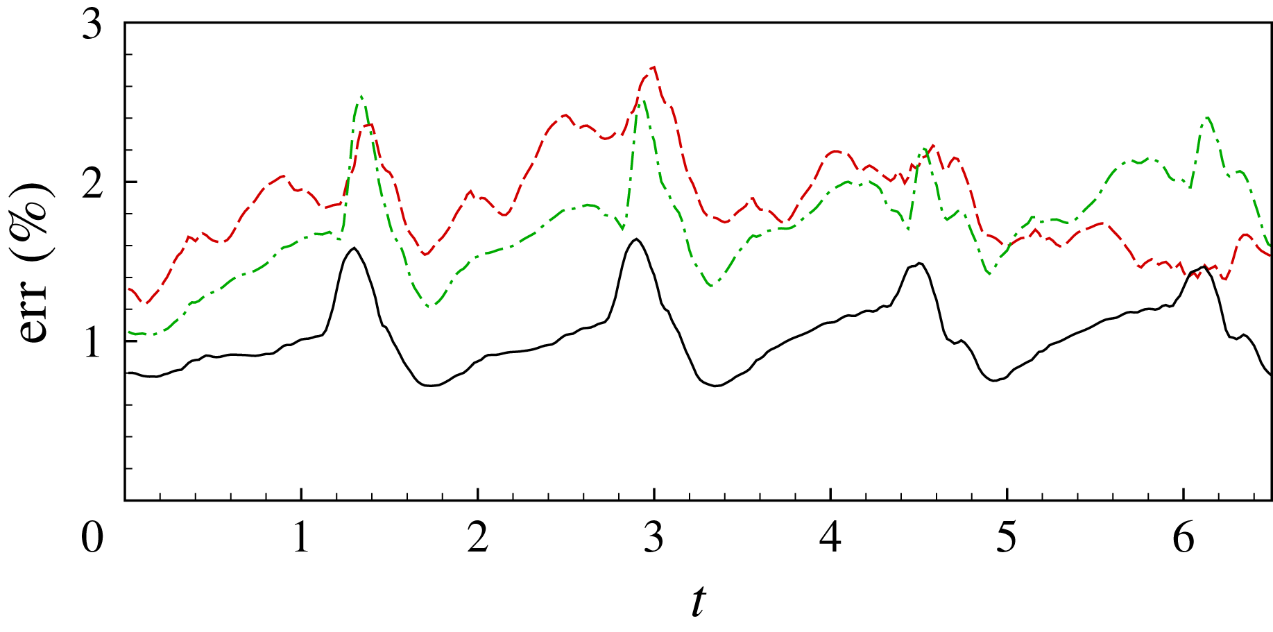
Errors of ROMs: red dashed line, 11 modes; green dashed-dotted line, 15 modes; black solid line, 21 modes.

Figure 12.

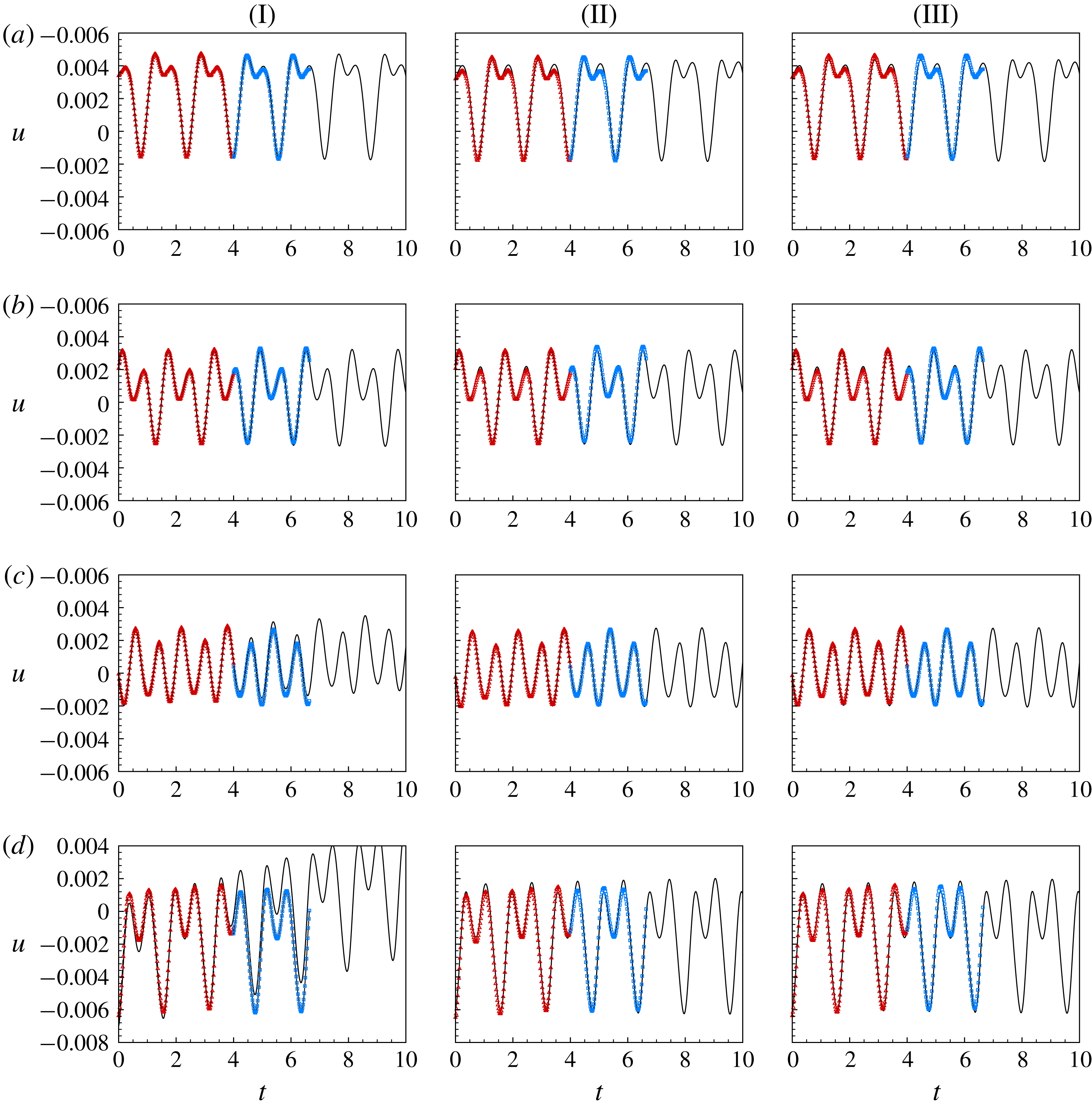
Time evolution of streamwise velocity $u$ given by ROMs with 11, 15 and 21 modes (I–III) at $x=5.275$ , 5.542, 5.803 and 6.058, $y=0.01$ , $z=0.175$ (a–d), respectively: — △ —, TRI; — ◻ —, TRO; ——, ROM.

To quantify the prediction error of the ROMs, we define the averaged relative error as follows:

(3.3) $$\begin{eqnarray}\displaystyle \text{err}(t)=\frac{\left(\displaystyle \mathop{\sum }_{i=1}^{N}|a_{i}(t)-a_{pi}(t)|^{2}/N\right)^{1/2}}{\left(\displaystyle \mathop{\sum }_{i=1}^{N}a_{pi}(t)^{2}\right)^{1/2}}, & & \displaystyle\end{eqnarray}$$

where $N$ is the number of modes, and $a_{pi}$ represents the projected DNS data on POD mode $i$ . As shown in figure 11, the relative error is less than 3 % in all cases, and generally decreases when more modes are used in the ROMs. Notably, however, the relative error with 15 modes is larger than that with 11 modes at some temporal instants, especially near the peaks and in the TRO region. This is caused by the inaccurate prediction of the higher modes as discussed above.

Flow reconstruction is performed to further verify the ROMs. The temporally evolving POD modes are added together to obtain the predicted flow fields. The streamwise velocity $u$ given by the ROMs with 11, 15 and 21 modes is compared with the original DNS data at four selected points at $x=5.275$ , 5.542, 5.803 and 6.058, $y=0.01$ , $z=0.175$ inside the boundary layer. As shown in figure 12(I-a) to (I-d) for the ROM with 11 modes, the velocity $u$ at $x=5.275$ , 5.542 and 5.803 can be accurately predicted, while further downstream at $x=6.058$ , where the transition is about to take place, the discrepancy is obvious between the predicted and DNS data. This suggests that in the transition region the nonlinear effects become stronger and the flow more complex, and more modes are needed to construct a ROM capable of sufficiently accurate prediction. Increasing the modes used to 15 and 21, the prediction at $x=6.058$ becomes more accurate, as seen in figure 12(II-d) and (III-d). Besides the streamwise velocity $u$ , the other flow quantities (not shown here) behave similarly. Thus, the reconstructed flow field confirms the accuracy of the ROMs.

The prediction error is also computed for the reconstructed $u$ at $x=6.058$ , defined as

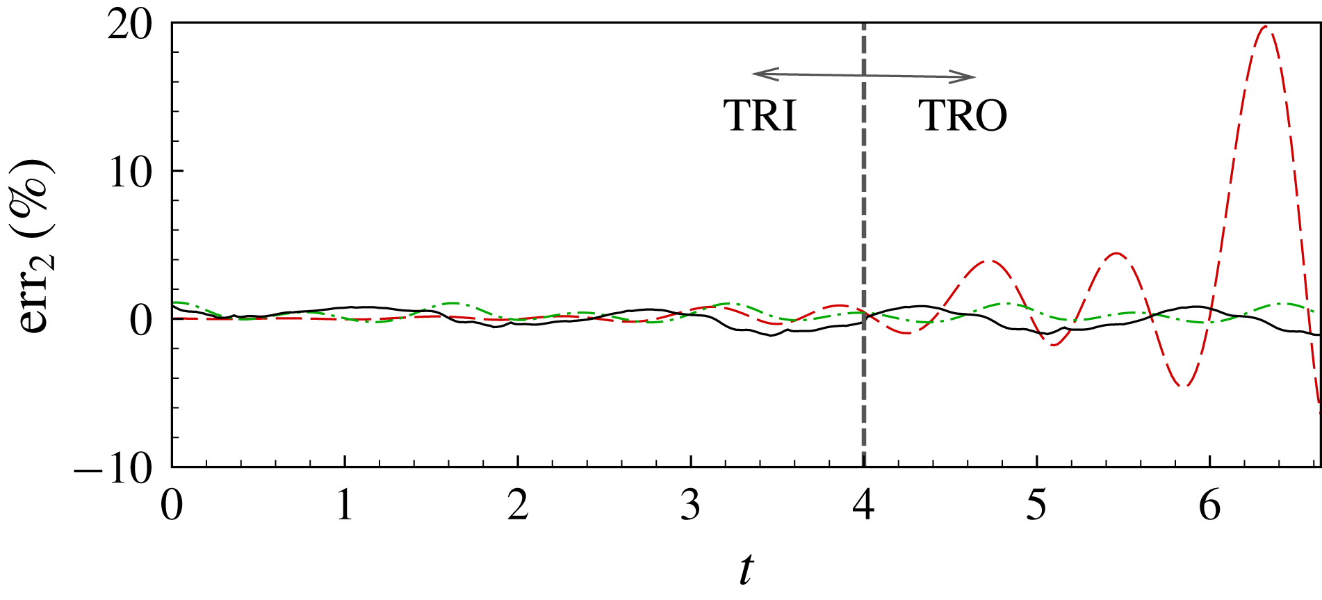
(3.4) $$\begin{eqnarray}\displaystyle \text{err}_{2}(t)=\frac{\left|u(t)-\displaystyle \mathop{\sum }_{i}^{N}b_{i}(t)u_{i}\right|}{u_{rms}}\times 100\,\%. & & \displaystyle\end{eqnarray}$$

The results are shown in figure 13. The relative errors in the TRI for the three ROMs are small enough to be neglected. For the 11-mode ROM, the prediction error rises rapidly in the TRO, indicating that the ROM is unstable there. When the mode number in the ROM increases to 15 and 21, the error is reduced to below 2 %.

Figure 13.

Errors of ROMs for the reconstructed $u$ at $x=6.058$ : red dashed line, ROM with 11 modes; green dashed-dotted line, ROM with 15 modes; black solid line, ROM with 21 modes.

The stability of the ROMs can be determined from the real component of the eigenvalues of their temporal evolution matrix, which is referred to as the amplification rate in the following. The eigenvalues of the 11-, 15- and 21-mode ROMs considered herein were calculated and the largest amplification rates are listed in table 2. All of the eigenvalues are positive, indicating that all three ROMs are unstable. However, the largest amplification rate decreases as the order (number of modes) increases. Hence, although the absolute stability of the truncated ROMs cannot be guaranteed, increasing their order reduces the prediction error and prolongs the time period in which valid predictions can be made, as shown by figure 3 and table 2.

Table 2.

Largest amplification rates of the ROMs.

It is instructive to discuss the CPU times needed to obtain the ROMs and the computational savings of using this model. The computational time in this study includes solving the DNS, POD and DMD equations and the temporal evolution ODEs for the ROM. The cost of the first three procedures is independent of ROM size, while the last requires relatively little CPU time. An estimation of the CPU time costs for each procedure is listed below:

1. (i) CPU information: Intel(R) Xeon(R) CPU E5-2683 v3 @ 2.00 GHz.

2. (ii) DNS: approximately 15 CPU seconds multiplied by 24 cores per time step.

3. (iii) POD and DMD: approximately 9000 CPU seconds.

4. (iv) ROM (less than 30 modes): less than 6.0 CPU seconds for 100 000 steps.

To simulate 10 000 time steps, DNS would cost 3.6 million CPU seconds. However, for the ROM, the CPU time cost would be only 9000 CPU seconds for the POD and DMD procedures combined, which is much lower than that of DNS.