





1. Introduction
Wave kinetic theory describes the long-time statistical evolution of weakly nonlinear dispersive waves, predicting irreversible spectral transfer towards either a thermal equilibrium state or a Kolmogorov–Zakharov (KZ) cascade (e.g. Nazarenko Reference Nazarenko2011; Zakharov et al. Reference Zakharov, L’vov and Falkovich2012). While this theory is well developed for deep-water waves, beginning with Hasselmann’s derivation of the wave kinetic equation (WKE) (Hasselmann Reference Hasselmann1962), its shallow-water counterpart is less understood in the literature. For two-dimensional (2-D) shallow-water surface waves, the theory has been studied starting from either the Euler equations (Zakharov Reference Zakharov1999) or the Boussinesq equations (Onorato et al. Reference Onorato, Osborne, Janssen and Resio2009), with their predictions of the KZ spectrum observed in wave tank experiments (Kaihatu et al. Reference Kaihatu, Veeramony, Edwards and Kirby2007) and in detailed numerical studies (Clark di Leoni et al. Reference Clark di Leoni, Cobelli and Mininni2014). However, in the one-dimensional (1-D) setting, there is currently no established theory for wave turbulence, as many contend the dynamics can be described by integrable models (Zakharov et al. Reference Zakharov, L’vov and Falkovich2012), such as the Korteweg–de Vries (KdV), Kadomtsev–Petviashvili-2, Camassa–Holm and Kaup–Boussinesq (KB) equations. This line of reasoning is due in part to the widely held empirical belief that integrable systems do not admit non-trivial kinetic descriptions (e.g. Zakharov & Schulman Reference Zakharov and Schulman1980, Reference Zakharov and Schulman1988; Zakharov Reference Zakharov1991).
The purpose of this paper is to revisit the largely underexplored problem of wave turbulence in bidirectional 1-D shallow-water waves, starting from the
 $abcd$
class of Boussinesq equations, which provide descriptions of the dynamics in the long-wave regime. This class includes the completely integrable KB equation (e.g. Kaup Reference Kaup1975; Kupershmidt Reference Kupershmidt1985; El et al. Reference El, Grimshaw and Pavlov2001; Ivanov Reference Ivanov2009; Bhrawy et al. Reference Bhrawy, Tharwat and Abdelkawy2013; Gong & Wang Reference Gong and Wang2022; Klein & Saut Reference Klein and Saut2025), as well as several well-known non-integrable models such as the classical Boussinesq, Bona–Smith and Benjamin–Bona–Mahony systems (e.g. Bona, Chen & Saut Reference Bona, Chen and Saut2002, Reference Bona, Chen and Saut2004). From an experimental perspective, studies of bidirectional shallow-water waves (e.g. Redor et al. Reference Redor, Barthélemy, Michallet, Onorato and Mordant2019, Reference Redor, Michallet, Mordant and Barthélemy2021; Leduque et al. Reference Leduque, Kaczmarek, Michallet, Barthélemy and Mordant2025) have demonstrated a range of behaviours, including spectral evolution towards a flat energy spectrum at large scales (interpreted as Rayleigh–Jeans (RJ) distribution in Pelinovsky & Sergeeva (Kokorina) (Reference Pelinovsky and Sergeeva (Kokorina)2006)) and/or the emergence of a soliton gas, depending on the system nonlinearity and forcing condition. These observations suggest that it is problematic to view either the completely integrable KB equation or standard non-integrable Boussinesq equations as a standalone, canonical model for 1-D bidirectional shallow-water waves, as each only accounts for a subset of the results, i.e. integrable features in the former and more traditional wave kinetic behaviour in the latter.
To develop a comprehensive understanding of both integrable and non-integrable dynamics, we consider the completely integrable KB equation and a truncated-dispersion variant representing the non-integrable setting. Although exact dispersion relations differ across the
 $abcd$
class, this truncation retains the common leading-order long-wave dispersive behaviour. A normal-form transformation can be applied to the models considered to remove the quadratic terms, for which we carefully characterise its validity condition depending on the parameters
 $\alpha$
and
 $\beta$
measuring the nonlinearity and dispersion. This yields an interaction coefficient of the same general form for both cases, differing only in the dispersion relation. For the KB equation, we numerically confirm that the interaction coefficient is zero exactly on the four-wave resonant manifold, consistent with the prevailing view in the literature (e.g. Zakharov & Schulman Reference Zakharov and Schulman1980, Reference Zakharov and Schulman1988; Zakharov Reference Zakharov1991). In contrast, when considering the truncated-dispersion model, our analysis yields a non-zero interaction coefficient that can be reduced to a compact form, clearly demonstrating non-trivial wave kinetics. The resulting WKE is inherently non-homogeneous due to the inhomogeneity of the dispersion relation. While the thermal equilibrium spectra remain as exact stationary solutions, the KZ solutions must be derived under approximations in a novel way. We derive two distinct direct cascade solutions corresponding to the limits of small and large modal amplitudes at low wavenumbers, given respectively by
 $n_k\sim |k|^{-3}$
and
 $n_k\sim |k|^{-3/2}$
, with each corresponding to a local solution of the WKE.
We proceed to perform direct numerical simulations, both to test the validity of our theoretical predictions and to investigate the underlying mechanism of energy transfer. We start by demonstrating a free-evolution case of the KB equation from random-wave initial conditions, where the discrete eigenvalues obtained from the direct scattering transform (representing solitons present in the initial field) remain constant in time, while the wavenumber spectrum quickly evolves towards a state consistent with the RJ scaling. This case demonstrates that, despite the KB equation being completely integrable and maintaining isospectrality of the eigenvalues, it can still exhibit significant spectral evolution due to quasi-resonant triad interactions. We then turn to simulations of the forced-dissipated non-integrable Boussinesq equation, where the low-wavenumber modal amplitude is controlled through the presence of the low-wavenumber dissipation. For small and large modal amplitudes at low wavenumbers, respectively, we reproduce the two theoretical KZ solutions. We also discuss how wave kinetic behaviour may become possible even in the full KB model as a result of four-wave quasi-resonant interactions. This is due to the previously unidentified near-singular behaviour of the interaction coefficient near the resonant manifold. A more detailed study is left for future work.
We finally remark that the wave kinetic behaviour we discover in the present paper is fundamentally different from Janssen’s WKE for the 1-D nonlinear Schrödinger equation (Janssen Reference Janssen2003), as well as the notion of ‘integrable turbulence’ (e.g. Agafontsev & Zakharov Reference Agafontsev and Zakharov2015, Reference Agafontsev and Zakharov2016; Randoux et al. Reference Randoux, Walczak, Onorato and Suret2016; Roberti et al. Reference Roberti, El, Randoux and Suret2019; El Reference El2021; Bonnemain et al. Reference Bonnemain, Doyon and El2022; Suret et al. Reference Suret, Randoux, Gelash, Agafontsev, Doyon and El2024). The former describes a time-dependent collision integral that vanishes as
 $t\rightarrow \infty$
(thus saturating to a steady-state spectrum), whereas the latter may refer to a soliton-gas state in an integrable model, described statistically by a kinetic theory for the ensemble of solitons. It is often assumed that the soliton-gas state is the only physically relevant phenomenon for 1-D shallow-water waves. Our results demonstrate that this is not the case, as free-wave, non-resonant interactions and spectral transfer may occur in a more traditional wave-turbulence sense, providing insight into integrable systems in a broader context. Taken together with the non-integrable Boussinesq case, which supports true resonant interactions and a non-trivial WKE, these results establish a robust theoretical framework for 1-D shallow-water wave turbulence.
2. Theoretical derivation
2.1. Derivation of the wave kinetic equation
In this section, we use the KB equation as a starting point to develop a generalised framework that we apply to two representative cases within the
 $abcd$
class of Boussinesq equations. The resulting normal-form interaction coefficient has the same general structure in these cases, with the dispersion relation being the only model-dependent component. We examine the interaction coefficient for both the full KB variant and its truncated-dispersion version.
The dimensional KB system is given by
 \begin{align} \eta _t + [(h+\eta )u]_x=-\frac {h^3}{3}u_{xxx}, \\[-28pt] \nonumber \end{align}
 \begin{align} u_t+uu_x+g\eta _x=0, \\[0pt] \nonumber \end{align}
where
 $\eta (x,t)$
denotes the surface elevation,
 $u(x,t)$
is the fluid velocity,
 $g$
is the acceleration of gravity and
 $h$
is the water depth. The system of (2.1) and (2.2) is known to be completely integrable in the inverse scattering method sense (Kaup Reference Kaup1975). We introduce the following non-dimensional variables:
 \begin{align} \begin{gathered} \tilde {\eta } = \eta / a, \quad \tilde {x} = x / L_p,\quad \tilde {t} = t / (L_p / \sqrt {gh}), \quad \tilde {u} = u /\left(\sqrt {gh} \frac {a}{h}\right) \!. \end{gathered} \end{align}
where
 $a$
denotes the characteristic wave amplitude (e.g. half the significant wave height
 $H_s$
) and
 $L_p$
is the peak wavelength of the wave field. Substituting (2.3) into (2.1) and (2.2) and omitting the tilde notation, we obtain
 \begin{align} \eta _t + u_x + \alpha (\eta u)_x = -\frac {1}{3}\beta u_{xxx}, \\[-28pt] \nonumber \end{align}
 \begin{align} u_t+\eta _x+\alpha uu_x=0, \\[0pt] \nonumber \end{align}
where
 $\alpha = a/h$
and
 $\beta = (h/L_p)^2$
are dimensionless measures of nonlinearity and dispersion, respectively.
We consider (2.4) and (2.5) on a periodic domain
 $\mathbb{T}_L$
. Defining Fourier-domain variables such as
 $\hat {\eta }_k(t)=\int _0^L \eta (x,t) {\rm e}^{-ikx}\, {\rm d}x/L$
(note that
 $k$
can be positive or negative), (2.4) and (2.5) can be transformed into
 \begin{align} \frac {\partial \hat {\eta }_k}{\partial t} + i\left(k-\frac {1}{3}\beta k^3\right) \hat {u}_k + i\alpha \sum _{k_1+k_2=k} k \hat {\eta }_{k_1} \hat {u}_{k_2} = 0, \\[-28pt] \nonumber \end{align}
 \begin{align} \frac {\partial \hat {u}_k}{\partial t} + ik \hat {\eta }_k + \frac {i}{2} \alpha \sum _{k_1+k_2=k} k \hat {u}_{k_1} \hat {u}_{k_2} =0. \\[0pt] \nonumber \end{align}
The linear part of (2.6) and (2.7) yields the dispersion relation
 \begin{align} \omega _k = \kappa \sqrt {1-\frac {1}{3}\beta \kappa ^2}, \end{align}
where
 $\kappa = |k|$
. Assuming
 $\beta \kappa ^2 \ll 1$
, we expand in the small parameter
 $\beta \kappa ^2$
and retain terms through first order:
 \begin{align} \omega _k=\kappa \left (1-\frac {\beta }{6}\kappa ^2\right )\!. \end{align}
This approximation defines the truncated-dispersion variant of (2.6) and (2.7), whereas the same equations with the full dispersion relation (2.8) are referred to as the full KB equation. This truncated form captures the leading-order dispersive behaviour of non-integrable models in the
 $abcd$
class (e.g. Bona et al. Reference Bona, Chen and Saut2002, Reference Bona, Chen and Saut2004). Both (2.8) and (2.9) agree with the shallow-water dispersion relation
 $\omega _k=\kappa$
when
 $\beta \kappa ^2\ll 1$
, but depart significantly from it on the descending branch:
 \begin{align} \kappa \gt \kappa _*,\qquad \frac {{\rm d}\omega }{{\rm d}\kappa }\Big |_{\kappa =\kappa _*}=0, \end{align}
where
 $\kappa _*=\sqrt {3/(2\beta )}$
for the full KB equation and
 $\kappa _*=\sqrt {2/\beta }$
for the truncated variant. In practice, we limit to a finite wavenumber range
 $\kappa _{\textit{max}}\lt \kappa _*$
, omitting the descending branch to ensure we remain in the near-shallow-water regime for the subsequent theoretical and numerical analyses.
By defining the canonical variables
 \begin{align} \hat {\eta }_k = \frac {\sqrt {2}}{2}\omega _k^{1/2} \big(a_k + a_{-k}^* \big) \end{align}
and
 \begin{align} \hat {u}_k = \frac {\sqrt {2}}{2}\frac {k}{\omega _k^{1/2}} \big(a_k - a_{-k}^* \big), \end{align}
leading to
 \begin{align} a_k = \frac {\sqrt {2}}{2}\omega _k^{-1/2}\hat {\eta }_k + \frac {\sqrt {2}}{2} \frac {\omega _k^{1/2}}{k}\hat {u}_k, \end{align}
we can diagonalise (2.6) and (2.7) in the variable
 $a_k$
:
 \begin{align} \frac {\partial a_k}{\partial t} + i\omega _k a_k + \frac {i\alpha }{4\sqrt {2}} &\sum _{k_1+k_2=k} \left\{ U_{k12}a_{k_1}a_{k_2} - U_{k12}a_{k_1}a_{-k_2}^* \right. \nonumber \\[5pt]& \left. +S_{k12}a_{-k_1}^*a_{k_2} - S_{k12} a_{-k_1}^*a_{-k_2}^* \right\} = 0, \end{align}
where
 \begin{align} U_{k12}= [2W(k,2)+W(1,2)] (\omega _{k}\omega _{k_1}\omega _{k_2})^{1/2}, \\[-12pt] \nonumber \end{align}
 \begin{align} S_{k12}= [2W(k,2)-W(1,2)] (\omega _{k}\omega _{k_1}\omega _{k_2})^{1/2}, \\[10pt] \nonumber \end{align}
with
 \begin{align} \begin{aligned} W(k,j)=\frac {kk_j}{\omega _{k}\omega _{k_j}},\qquad W(i,j)=\frac {k_ik_j}{\omega _{k_i}\omega _{k_j}}. \end{aligned} \end{align}
Manipulating (2.14) using symmetry conditions, we get the final canonical equation:
 \begin{align} \frac {\partial a_k}{\partial t} + i\omega _k a_k + &i \left\{\sum _{k_1+k_2=k} V_{k12} a_{k_1}a_{k_2} + \sum _{k_1-k_2=k} V_{k12} a_{k_1}a_{k_2}^* \right. \nonumber \\[5pt] & \left.+ \sum _{k_2-k_1=k} V_{k12} a_{k_1}^*a_{k_2} + \sum _{k_2+k_1+k=0} V_{k12} a_{k_1}^*a_{k_2}^* \right\} = 0, \end{align}
where
 \begin{align} V_{k12}=&\frac {\alpha (\omega _{k}\omega _{k_1}\omega _{k_2})^{1/2}}{4\sqrt {2}}[W(k,1)+W(k,2)+W(1,2)]. \end{align}
We note that all interaction kernels in (2.18) are the same, which is consistent with the case in the 2-D Boussinesq equation derived in Onorato et al. (Reference Onorato, Osborne, Janssen and Resio2009).
Our next goal is to apply a normal-form transformation (or multiple time scale method) to (2.18) with the aim of eliminating the quadratic nonlinear terms, since the dispersion relation (2.8) does not support triad resonant interactions. This approach has been previously applied to the 2-D Euler equations for shallow water (Zakharov Reference Zakharov1999) and to the 2-D Boussinesq equations (Onorato et al. Reference Onorato, Osborne, Janssen and Resio2009). The procedure is standard (e.g. Krasitskii Reference Krasitskii1994; Zakharov et al. Reference Zakharov, L’vov and Falkovich2012) except for the validity condition of the transformation, which is discussed later.
We proceed by applying the normal-form transformation method to introduce a new variable
 $b_k$
defined as
 \begin{align} \begin{split} a_k=\ b_k&+ \sum _{k_1+k_2=k} \varGamma ^{[1]}_{k12}b_{k_1}b_{k_2}- 2 \sum _{k_2-k_1=k} \varGamma ^{[1]}_{2k1}b_{k_1}^*b_{k_2}+ \sum _{k_1+k_2+k=0} \varGamma ^{[2]}_{k12}b_{k_1}^*b_{k_2}^*\\ &+\sum _{k+k_1=k_2+k_3} B_{k123} b_{k_1}^*b_{k_2}b_{k_3}+ \text{other cubic terms}, \end{split} \end{align}
such that, rewriting (2.18) in terms of
 $b_k$
and retaining terms up to cubic order, yields
 \begin{align} \frac {\partial b_k}{\partial t} + i\omega _k b_k + i\sum _{k+k_1=k_2+k_3} T_{k123} b_{k_1}^*b_{k_2}b_{k_3} = 0. \end{align}
This transformation is achieved by appropriately choosing the coefficients in (2.20), for example,
 \begin{align} \varGamma ^{[1]}_{k12} = \frac {-V_{k12}}{\omega _k-\omega _1-\omega _2},\quad \varGamma ^{[2]}_{k12} = \frac {-V_{k12}}{\omega _k+\omega _1+\omega _2}. \end{align}
The interaction kernel in (2.21) is given by
 \begin{align} \begin{split} T_{k123} =&-V_{k,2,k-2}V_{3,1,3-1}\Big [\frac {1}{\omega _2+\omega _{k-2}-\omega _k} + \frac {1}{\omega _1+\omega _{3-1}-\omega _3} \Big ] \\[4pt]& -V_{1,2,1-2}V_{3,k,3-k}\Big [\frac {1}{\omega _2+\omega _{1-2}-\omega _1} + \frac {1}{\omega _k+\omega _{3-k}-\omega _3} \Big ] \\[4pt]& -V_{k,3,k-3}V_{2,1,2-1}\Big [\frac {1}{\omega _3+\omega _{k-3}-\omega _k} + \frac {1}{\omega _1+\omega _{2-1}-\omega _2} \Big ] \\[4pt]& -V_{1,3,1-3}V_{2,k,2-k}\Big [\frac {1}{\omega _3+\omega _{1-3}-\omega _1} + \frac {1}{\omega _k+\omega _{2-k}-\omega _2} \Big ] \\[4pt]& -V_{k+1,k,1}V_{2+3,2,3}\Big [\frac {1}{\omega _{k+1}-\omega _k-\omega _1} + \frac {1}{\omega _{2+3}-\omega _2-\omega _3} \Big ] \\[4pt]& -V_{-k-1,k,1}V_{-2-3,2,3}\Big [\frac {1}{\omega _{k+1}+\omega _k+\omega _1} + \frac {1}{\omega _{2+3}+\omega _2+\omega _3} \Big ]. \end{split} \end{align}
We observe that
 $T_{k123}$
in (2.23) possesses the desired symmetry properties, namely
 $T_{k123}=T_{1k23}=T_{k132}=T_{23k1}$
.
To obtain the above results, the transformation
 $a_k \rightarrow b_k$
defined in (2.20) must be near-identity. As discussed in Zakharov (Reference Zakharov1999), this requires
 \begin{align} \begin{split} \Big |\sum _{k_1+k_2=k} \varGamma ^{[1]}_{k12}b_{k_1}b_{k_2} - 2 \sum _{k_2-k_1=k} \varGamma ^{[1]}_{2k1}b_{k_1}^*b_{k_2}+ \sum _{k_1+k_2+k=0} \varGamma ^{[2]}_{k12}b_{k_1}^*b_{k_2}^* \Big | \ll |b_k|. \end{split} \end{align}
In formulating (2.24), inconsistencies arise in Zakharov (Reference Zakharov1999). In particular, the analysis in Zakharov (Reference Zakharov1999) does not account for the random phases of
 $b_k$
when estimating the summations on the left-hand side, resulting in an overestimation. In Appendix A, we provide a new estimation that properly incorporates phase randomness to derive the validity condition for the normal-form transformation (see also Wu et al. Reference Wu, Onorato, Hani and Pan2025). The result is straightforward and can be summarised as follows:
We consider a spectrum with finite bandwidth
 $\varDelta$
in
 $k$
, assuming that it decays sufficiently fast outside
 $\varDelta$
. Then (
2.24
) corresponds to the condition of
 $\alpha \ll \beta$
. While the detailed derivation is provided in Appendix A, the underlying logic is to avoid small denominators arising on the left-hand side of (2.24). The most singular term in the denominator is of
 $O(\beta )$
, which must be significantly larger than the numerator of
 $O(\alpha )$
.
Starting from (2.21), we formally derive the corresponding WKE following standard procedures (e.g. Nazarenko Reference Nazarenko2011). The WKE is given by
 \begin{align} \begin{split} \frac {\partial n_k}{\partial t} =\ &4\pi \int |T_{k123}|^2 n_kn_1n_2n_3 \left [ \frac {1}{n_k}+\frac {1}{n_1}-\frac {1}{n_2}-\frac {1}{n_3} \right ]\\[5pt]&\times \delta (k+k_1-k_2-k_3)\delta (\omega _k+\omega _1-\omega _2-\omega _3) \,{\rm d}k_1\,{\rm d}k_2\,{\rm d}k_3, \end{split} \end{align}
where
 $n_k=\langle b_kb_k^*\rangle$
denotes the wave action, with
 $\langle a_ka_k^*\rangle =\langle b_k b_k^*\rangle +O(\alpha ^2)$
.
To determine whether (2.25) is trivial or not, it is essential to analyse the interaction coefficient
 $T_{k123}$
on the resonant manifold defined by the resonance condition in (2.25). We begin by emphasising that for any concave-down dispersion relation, such as (2.8) and (2.9), the resonance condition in frequency
 $\omega$
cannot be satisfied if all wavenumbers involved share the same sign (i.e. all positive or all negative). Non-trivial resonant interactions occur only when one wavenumber has the opposite sign to the other three (e.g. one negative and three positive), or when two wavenumbers are positive and two are negative. The two-positive-two-negative configuration, however, requires at least one large wavenumber on the descending branch (2.10). Since both models have deviated substantially from the true shallow-water dispersion in this range, these interactions lie outside the regime of interest (i.e.
 $\kappa \gt \kappa _{\textit{max}}$
), and are therefore regarded as spurious solutions that may be discarded. A graphical proof of the resonance configurations, exemplified using (2.9), is provided in Appendix B, and is fundamental to the subsequent analysis of
 $T_{k123}$
.
We begin our analysis with the KB equation with the dispersion relation (2.8). According to the literature (e.g. Zakharov & Schulman Reference Zakharov and Schulman1980, Reference Zakharov and Schulman1988; Zakharov Reference Zakharov1991), we expect this system to yield a trivial interaction coefficient on the resonant manifold due to its complete integrability. Proving the coefficient vanishes on the resonant manifold for (2.8) is non-trivial, as the manifold lacks a simple analytical expression due to the square root. The next best approach is to verify numerically whether (2.23) vanishes on the resonant manifold. To this end, we compute
 $T_{k123}$
for a large number of resonant quartets using the dispersion relation (2.8), with all computations carried out using quadruple precision. Table 1 presents a subset of these quartets tracing the resonant manifold, demonstrating that the resulting coefficient vanishes to numerical precision, which implies that the KB equation yields a trivial WKE.
Values of the interaction coefficient
 $T_{k123}$
for the KB equation using
 $\beta =0.001$
for different resonant quartets.

Table 1. Long description
A table showing values of the interaction coefficient for the KB equation using different resonant quartets. The table has 9 rows and 5 columns. The columns are labeled k, k1, k2, k3, and |T123|. The table presents the following data: Row 1: k, 5.0; k1, 1.982387; k2, 7.0; k3, -1.76 x 10^-2; |T123|, 4.66 x 10^-32. Row 2: k, 5.0; k1, 2.969726; k2, 8.0; k3, -3.03 x 10^-2; |T123|, 4.47 x 10^-31. Row 3: k, 5.0; k1, 3.954433; k2, 9.0; k3, -4.56 x 10^-2; |T123|, 6.76 x 10^-31. Row 4: k, 5.0; k1, 4.936444; k2, 10.0; k3, -6.36 x 10^-2; |T123|, 3.50 x 10^-31. Row 5: k, 5.0; k1, 5.915683; k2, 11.0; k3, -8.43 x 10^-2; |T123|, 4.36 x 10^-31. Row 6: k, 5.0; k1, 6.892058; k2, 12.0; k3, -1.08 x 10^-1; |T123|, 7.05 x 10^-31. Row 7: k, 5.0; k1, 7.865463; k2, 13.0; k3, -1.35 x 10^-1; |T123|, 2.63 x 10^-31. Row 8: k, 5.0; k1, 8.835773; k2, 14.0; k3, -1.64 x 10^-1; |T123|, 4.30 x 10^-31. Row 9: k, 5.0; k1, 9.802847; k2, 15.0; k3, -1.97 x 10^-1; |T123|, 1.58 x 10^-31. Row 10: k, 5.0; k1, 10.766521; k2, 16.0; k3, -2.33 x 10^-1; |T123|, 1.86 x 10^-31.
Next, we move on to the analytical calculation for the non-integrable Boussinesq variant with dispersion relation (2.9). The existing view for the shallow-water wave interaction coefficient, such as (2.23), is that it contains both near-singular and regular terms (Zakharov Reference Zakharov1999; Onorato et al. Reference Onorato, Osborne, Janssen and Resio2009). The former correspond to frequency mismatches of
 $O(\beta )$
(i.e. their inverses are of
 $O(1/\beta )$
, which is near-singular), while the latter are of
 $O(1)$
. It has previously been thought that the near-singular terms dominate the coefficient
 $T_{k123}$
. However, the near-singular versus regular terms need to be evaluated through a much more delicate analysis, which we perform below.
Without loss of generality, we consider
 $k,k_1,k_2$
to be positive and
 $k_3$
to be negative, such that
 $\kappa _2 \gt \kappa , \kappa _1, \kappa _3$
. Under this assumption, the ‘near-singular’ and ‘regular’ terms in (2.23) (hereafter named as
 $T_{{I}}$
and
 $T_{\textit{II}}$
) can be collected as
 \begin{align} T_{{I}} = -\frac {V_{k,3,k-3}V_{2,1,2-1}}{\omega _1+\omega _{2-1}-\omega _2} -\frac {V_{1,3,1-3}V_{2,k,2-k}}{\omega _k+\omega _{2-k}-\omega _2} -\frac {V_{k+1,k,1}V_{2+3,2,3}}{\omega _{k+1}-\omega _k-\omega _1}, \\[-28pt] \nonumber \end{align}
 \begin{align} T_{\textit{II}} = T_{k123}-T_{{I}}. \\[0pt] \nonumber \end{align}
Substitution of (2.9) and (2.19) into (2.26) gives (see details in Appendix C)
 \begin{align} T_{{I}} = -\frac {3\alpha ^2}{16\beta } \Big ( \frac {\kappa _3^3}{\kappa \kappa _1\kappa _2} \Big )^{1/2}, \\[-28pt] \nonumber \end{align}
 \begin{align} T_{\textit{II}}= -\frac {\alpha ^2}{64} (\kappa \kappa _1\kappa _2\kappa _3)^{1/2} \left [\kappa _3\left (\frac {1}{\kappa _1}-\frac {1}{\kappa _2}+\frac {1}{\kappa }\right )\right ]. \\[-12pt] \nonumber \end{align}
At first glance, the relative magnitude of these two contributions in the small-
 $\beta$
limit is not immediately clear from (2.27a,b
). However, solving the resonance condition in (2.25) gives
 $\kappa _3=(\beta /4) \kappa \kappa _1 \kappa _2$
(see Appendix D); substituting this into (2.27a,b
) yields
 \begin{align} T_{{I}} = -\frac {3\alpha ^2}{128}\beta ^{1/2}\kappa \kappa _1\kappa _2, \\[-28pt] \nonumber \end{align}
 \begin{align} T_{\textit{II}} = -\frac {\alpha ^2}{512}\beta ^{3/2}\kappa \kappa _1\kappa _2 (\kappa \kappa _2+\kappa _1\kappa _2-\kappa \kappa _1). \\[-12pt] \nonumber \end{align}
Thus, for small
 $\beta$
, the
 $T_{{I}}$
dominates, and the total coefficient can be reduced to the compact leading-order form
 \begin{align} T_{k123}\approx T_{{I}}=-\frac {3\alpha ^2}{128}\beta ^{1/2}\kappa \kappa _1\kappa _2. \end{align}
We note that if any wavenumber other than
 $k_3$
is chosen to be negative (with the others positive), the coefficient
 $T_{k123}$
can be directly evaluated using its symmetry properties. For example, if
 $k_1\lt 0$
, one can use the relation
 $T_{k123}=T_{231k}$
, where the latter evaluates to
 $T_{231k}=-(3\alpha ^2/128)[\sqrt {\beta }\kappa \kappa _2\kappa _3]$
. Consequently, a general expression for
 $T_{k123}$
can be written as
 \begin{align} T_{k123} = -\frac {3\alpha ^2}{128} \Big (\sqrt {\beta }\kappa _{\textit{mul}}\Big ), \end{align}
where
 $\kappa _{\textit{mul}}$
represents the multiplication of the magnitudes of the three wavenumbers with the same sign.
We also remark here that it is claimed in Zakharov (Reference Zakharov1999) that all ‘near-singular’ terms in
 $T_{k123}$
cancel out, based on the formulation from the Euler equation. This claim is in fact not relevant to the present case, since Zakharov (Reference Zakharov1999) assumes that all wavenumbers share the same sign, which is not consistent with the resonant manifold in (2.25).
Since
 $T_{k123}\neq 0$
on the resonant manifold according to (2.30), we have obtained a non-trivial WKE (2.25) from (2.4) and (2.5) with a truncated-dispersion relation approximation. Next, we seek stationary solutions to (2.25). The first set of stationary solutions is of RJ type, namely the equipartition-of-action solution
 $n_k\sim \kappa ^0$
and the equipartition-of-energy solution
 $n_k\sim 1/\omega _{k}\cong 1/\kappa ^{1}$
. These naturally hold for (2.25) since they turn the integrand in the integral on the right-hand side into zero at each point. However, the KZ turbulent solution to (2.25) needs to be found in a novel way, which we describe in the following section.
2.2. Kolmogorov–Zakharov spectra
One might attempt to find the KZ solution
 $n_k \sim \kappa ^\gamma$
to (2.25) using a ‘standard’ approach using the formula
 $\gamma =-2\tau /3 - 1$
(Nazarenko Reference Nazarenko2011) with
 $\tau$
the degree of homogeneity of
 $T_{k123}$
. However, this approach does not hold here because the dispersion relation (2.9) is inhomogeneous, which breaks the basis to derive the ‘standard’ formula. As one may have noticed here, even the degree of homogeneity
 $\tau$
is not certain here, depending on whether (2.27a,b
) or (2.28) is used for evaluation, which results from the same inhomogeneity issue. If one simply considers a dispersion relation
 $\omega _k=\kappa$
with
 $\beta =0$
, then the resonance condition leads to
 $\kappa _3=0$
in (2.27a,b
) so that
 $T_{k123}=0$
and the problem becomes trivial. Therefore, to obtain the KZ spectrum, we have to develop a refined approach which considers the cubic terms in the dispersion relation (as we have done in deriving (2.28)).
We start by considering an isotropic spectrum,
 $n_{-k}=n_k$
, which allows us to convert wavenumber
 $k$
into its magnitude
 $\kappa$
in (2.25). In particular, the resonance condition in
 $k$
permits eight sign choices for
 $k_1$
,
 $k_2$
and
 $k_3$
(for fixed positive
 $k$
), but disregarding trivial pairings (e.g.
 $k=k_2$
,
 $k_1=k_3$
;
 $k_1=k_2$
,
 $k=k_3$
) leaves only four non-trivial cases where the integrand is non-zero. The resulting equation in
 $\kappa$
is
 \begin{align} \frac {\partial n_\kappa }{\partial t} & = 4\pi \int |T_{k 123}|^2 n_\kappa n_1n_2n_3\left [ \frac {1}{n_\kappa }+\frac {1}{n_1}-\frac {1}{n_2}-\frac {1}{n_3} \right ]\delta (\omega _\kappa +\omega _1-\omega _2-\omega _3) \nonumber \\[5pt]& \quad \times \big [ \delta (\kappa +\kappa _1-\kappa _2+\kappa _3) +\delta (\kappa +\kappa _1+\kappa _2-\kappa _3)+\delta (\kappa -\kappa _1-\kappa _2-\kappa _3)\nonumber \\[5pt]& \quad +\delta (\kappa -\kappa _1+\kappa _2+\kappa _3)\big ] \,{\rm d}\kappa _1\,{\rm d}\kappa _2\,{\rm d}\kappa _3. \end{align}
We name the four terms in (2.31)
 $I_1$
,
 $I_2$
,
 $I_3$
and
 $I_4$
, corresponding to the four delta functions in the square brackets. To further simplify
 $I_1$
associated with
 $\delta (\kappa +\kappa _1-\kappa _2+\kappa _3)$
in (2.31) (as an example), we notice that the frequency resonance condition can be reduced to (see Appendix D.1)
 \begin{align} 0=\omega _\kappa +\omega _1-\omega _2-\omega _3\approx \kappa _3-\frac {\beta }{4}\kappa \kappa _1\kappa _2. \end{align}
The wavenumber resonance condition is reduced to
 $\kappa +\kappa _1-\kappa _2+O(\beta )=0$
, with the
 $O(\beta )$
term negligible at leading order. Therefore, integrating out the frequency condition and using (2.30) reduces
 $I_1$
to
 \begin{align} \begin{split} I_1=&\int \Big |\frac {3\alpha ^2}{128}\sqrt {\beta }\kappa \kappa _1\kappa _2\Big |^2 n_\kappa n_1n_2n_3\left [ \frac {1}{n_\kappa }+\frac {1}{n_1}-\frac {1}{n_2}-\frac {1}{n_3} \right ]\delta (\kappa +\kappa _1-\kappa _2)\,{\rm d}\kappa _1\,{\rm d}\kappa _2. \end{split} \end{align}
Following similar procedures, we can reduce
 $I_2$
and
 $I_3$
to
 \begin{align} \begin{split} I_2=&\int \Big |\frac {3\alpha ^2}{128}\sqrt {\beta }\kappa \kappa _1\kappa _3\Big |^2 n_\kappa n_1n_2n_3\left [ \frac {1}{n_\kappa }+\frac {1}{n_1}-\frac {1}{n_2}-\frac {1}{n_3} \right ]\delta (\kappa +\kappa _1-\kappa _3)\,{\rm d}\kappa _1\,{\rm d}\kappa _3 \end{split} \end{align}
and
 \begin{align} \begin{split} I_3=&\int \Big |\frac {3\alpha ^2}{128}\sqrt {\beta }\kappa \kappa _2\kappa _3\Big |^2 n_\kappa n_1n_2n_3\left [ \frac {1}{n_\kappa }+\frac {1}{n_1}-\frac {1}{n_2}-\frac {1}{n_3} \right ]\delta (\kappa -\kappa _2-\kappa _3)\,{\rm d}\kappa _2\,{\rm d}\kappa _3, \end{split} \end{align}
respectively. For
 $I_4$
, the frequency condition cannot be satisfied for
 $\kappa \sim O(1)$
, thus
 $I_4=0$
and does not contribute to (2.31).
Integrals (2.33)–(2.35) can be further simplified depending on the size of
 $n_\kappa$
at
 $\kappa \sim \beta$
relative to
 $n_\kappa$
in the inertial range. Here, the notation
 $\kappa \sim \beta$
refers to the low-wavenumber range where
 $n_\kappa$
is evaluated, not to the scaling of the wavenumbers retained in the reduced resonance condition. In what follows, we discuss two cases: Cases A and B with
 $n_\kappa$
respectively small and large in the vicinity of
 $\kappa \sim \beta$
. These two cases physically correspond to situations with and without large-scale damping in the simulations demonstrated in § 3.2.2.
2.2.1. Case A
Consider
 $I_1$
with
 $n_3\ll n_\kappa ,n_1,n_2$
. The integral in (2.33) can be reformulated as (with
 $1/n_3$
term dominating over other terms in the square bracket)
 \begin{align} I_1=-\int \Big |\frac {3\alpha ^2}{128}\sqrt {\beta }\kappa \kappa _1\kappa _2\Big |^2 n_\kappa n_1n_2\delta (\kappa +\kappa _1-\kappa _2)\,{\rm d}\kappa _1\,{\rm d}\kappa _2. \end{align}
Similar procedures applied to
 $I_2$
and
 $I_3$
reduce (2.34) and (2.35) to
 \begin{align} I_2=-\int \Big |\frac {3\alpha ^2}{128}\sqrt {\beta }\kappa \kappa _1\kappa _3\Big |^2 n_\kappa n_1n_3\delta (\kappa +\kappa _1-\kappa _3)\,{\rm d}\kappa _1\,{\rm d}\kappa _3 \end{align}
and
 \begin{align} I_3=\int \Big |\frac {3\alpha ^2}{128}\sqrt {\beta }\kappa \kappa _2\kappa _3\Big |^2 n_\kappa n_2n_3\delta (\kappa -\kappa _2-\kappa _3)\,{\rm d}\kappa _2\,{\rm d}\kappa _3. \end{align}
By defining
 \begin{align} R^\kappa _{12}=\Big |\frac {3\alpha ^2}{128}\sqrt {\beta }\kappa \kappa _1\kappa _2\Big |^2n_\kappa n_1n_2\delta (\kappa -\kappa _2-\kappa _1) \end{align}
the integral
 $I$
can be expressed as
 \begin{align} I=I_1+I_2+I_3=\int \big(R^\kappa _{12}-R^2_{1\kappa }-R^1_{\kappa 2} \big)\,{\rm d}\kappa _1\,{\rm d}\kappa _2. \end{align}
After applying the Zakharov transformations (Zakharov et al. Reference Zakharov, L’vov and Falkovich2012) and assuming a solution ansatz
 $n_\kappa \sim \kappa ^{-x}$
(see Appendix D.2 for full details), we can write (2.40) as
 \begin{align} I =\int R^\kappa _{12}\left [1-\Big (\frac {\kappa _1}{\kappa }\Big )^{3x-8}-\Big (\frac {\kappa _2}{\kappa }\Big )^{3x-8}\right]\,{\rm d}\kappa _1\,{\rm d}\kappa _2. \end{align}
The condition for a stationary solution is obtained by requiring the bracketed term to vanish, which leads to
 \begin{align} 3x-8=1 \;\Rightarrow \; x=3, \end{align}
which is the KZ exponent for Case A with small
 $n_\kappa$
at
 $\kappa \sim \beta$
.
In Appendix D.4, we further provide a locality analysis which leads to a locality window of
 $5/2\lt x\lt 4$
. The solution
 $x=3$
is therefore within the locality window and represents a valid local solution to the WKE.
2.2.2. Case B
Considering
 $n_3\gg n_\kappa ,n_1,n_2$
for
 $I_1$
and similar conditions for
 $I_2$
and
 $I_3$
, integrals (2.33)–(2.35) are reduced to
 \begin{align} \begin{split} I_1=&\int \Big |\frac {3\alpha ^2}{128}\sqrt {\beta }\kappa \kappa _1\kappa _2\Big |^2n_\kappa n_1n_2n_3 \left [ \frac {1}{n_\kappa }+\frac {1}{n_1}-\frac {1}{n_2} \right ]\delta (\kappa +\kappa _1-\kappa _2)\,{\rm d}\kappa _1\,{\rm d}\kappa _2, \end{split} \\[-12pt] \nonumber \end{align}
 \begin{align} \begin{split} I_2=&\int \Big |\frac {3\alpha ^2}{128}\sqrt {\beta }\kappa \kappa _1\kappa _3\Big |^2 n_\kappa n_1n_2n_3\left [ \frac {1}{n_\kappa }+\frac {1}{n_1}-\frac {1}{n_3} \right ]\delta (\kappa +\kappa _1-\kappa _3)\,{\rm d}\kappa _1\,{\rm d}\kappa _3 \end{split} \\[10pt] \nonumber \end{align}
and
 \begin{align} \begin{split} I_3=&\int \Big |\frac {3\alpha ^2}{128}\sqrt {\beta }\kappa \kappa _2\kappa _3\Big |^2 n_\kappa n_1 n_2n_3\left [ \frac {1}{n_\kappa }-\frac {1}{n_2}-\frac {1}{n_3} \right ]\delta (\kappa -\kappa _2-\kappa _3)\,{\rm d}\kappa _2\,{\rm d}\kappa _3. \end{split} \end{align}
Defining
 \begin{align} R^\kappa _{12}=\Big |\frac {3\alpha ^2}{128}\sqrt {\beta }\kappa \kappa _1\kappa _2\Big |^2n_\kappa n_1n_2n_3\left [ \frac {1}{n_\kappa }-\frac {1}{n_2}-\frac {1}{n_1} \right ]\delta (\kappa -\kappa _2-\kappa _1), \end{align}
and applying the Zakharov transformations with the solution ansatz
 $n_\kappa \sim \kappa ^{-x}$
(see Appendix D.3 for full details), we arrive at
 \begin{align} I =\int R^\kappa _{12}\left[1-\Big (\frac {\kappa _1}{\kappa }\Big )^{6x-8}-\Big (\frac {\kappa _2}{\kappa }\Big )^{6x-8}\right]\,{\rm d}\kappa _1\,{\rm d}\kappa _2. \end{align}
By enforcing the same condition as in § 2.2.1, we find that the stationary solution is obtained at
 \begin{align} 6x-8=1 \;\Rightarrow \; x=\frac {3}{2}, \end{align}
which is the KZ exponent for Case B with large
 $n_\kappa$
at
 $\kappa \sim \beta$
. The locality analysis in Appendix D.4 shows a locality window of
 $4/3\lt x\lt 5/2$
, so that this KZ solution is local.
3. Numerical study
A subsequent numerical study is performed with the purpose of verifying the theoretical results derived in § 2. In this section, we begin by outlining the methodology and numerical set-up implemented in this study. We then discuss the results from two scenarios, namely free-evolution and forced-dissipated configurations.
3.1. Methodology
We simulate the KB system (2.4) and (2.5) using a pseudospectral method paired with a fourth-order Runge–Kutta time marching scheme with an integration factor (IF-RK4) formulation (e.g. Pan Reference Pan2020). Key details of the scheme can be found in Appendix G, along with a validation against existing exact solutions of the KB system. All numerical experiments are performed on a computational domain of size
 $L = 2\pi$
with periodic boundary conditions, discretised using
 $N = 4096$
free wave modes (before de-aliasing). The value of
 $\beta$
is correspondingly chosen (and specified in each subsection) such that the high-order term in the dispersion relation in (2.8) is much smaller than the linear term, even for the highest wavenumber. In this section, we further present details of the numerical set-up for the free-evolution and forced-dissipated cases in §§ 3.2.1 and 3.2.2, respectively. We then introduce the formulation of the direct scattering transform (DST), as well as the numerical strategies to solve the spectral problem for the purpose of testing isospectrality for the KB model associated with its integrability.
3.1.1. Free-evolution configuration
All freely evolving cases are performed without external forcing and damping, using a Gaussian spectrum
 $S(\kappa )$
as the initial condition (e.g. Pelinovsky & Sergeeva (Kokorina) Reference Pelinovsky and Sergeeva (Kokorina)2006; Flamarion & Pelinovsky Reference Flamarion and Pelinovsky2024):
 \begin{align} S(\kappa )=Q\exp \bigg (-\frac {(\kappa -\kappa _p)^2}{2K^2}\bigg ), \end{align}
where
 $\kappa _p=512$
represents the wavenumber peak,
 $K=51.2$
characterises the spectral bandwidth and
 $Q$
is chosen such that the resulting data size is
 $\lesssim 1$
(say measured by
 $||\hat {\eta }_\kappa ||_\infty$
and
 $||\hat {u}_\kappa ||_\infty$
). The amplitude of each Fourier component
 $\hat {\eta }_\kappa$
is drawn from the spectrum
 $S(\kappa )$
. To construct a bidirectional field,
 $\hat {\eta }_\kappa$
is evenly split to equally distribute energy between left- and right-propagating components. Each component is assigned a random phase drawn uniformly from
 $(0,2\pi ]$
. The component
 $\hat {u}_\kappa$
is then obtained from
 $\eta _\kappa$
for both left- and right-propagating components via the linear relation. For all free-evolution experiments, we fix the dispersion parameter
 $\beta =0.2$
, and vary the nonlinearity parameter
 $\alpha$
to control the nonlinearity level.
3.1.2. Forced-dissipated configuration
All experiments begin from a quiescent initial state. Waves are excited by a forcing term
 $F(\kappa ,t)$
added to the right-hand side of (2.5) (or (2.7) defined in the spectral domain), in the form of (e.g. Dyachenko et al. Reference Dyachenko, Korotkevich and Zakharov2004; Pan Reference Pan2020; Zhang & Pan Reference Zhang and Pan2022b
; Korotkevich Reference Korotkevich2023)
 \begin{align} F(\kappa ,t)= \begin{cases} f_\kappa \exp \!\big [-C t + i(\omega _\kappa t + R)\big ], & t \leqslant T_c,\\[5pt]f_\kappa \exp \!\big [-C T_c +i(\omega _\kappa t + R)\big ], & t \gt T_c, \end{cases} \end{align}
with
 \begin{align} f_\kappa = \begin{cases} f_0 \frac {(\kappa -\kappa _1)(\kappa _2-\kappa )}{(\kappa _1-\kappa _2)^2}, & \kappa _1\leqslant \kappa \leqslant \kappa _2,\\[5pt]0, & \text{otherwise}, \end{cases} \end{align}
where
 $f_0=0.88$
controls the forcing amplitude (leading to a solution of size
 $O(1)$
and mitigating the finite-size effect; e.g. L’vov & Nazarenko Reference L’vov and Nazarenko2010; Hrabski & Pan Reference Hrabski and Pan2020; Zhang & Pan Reference Zhang and Pan2022a
),
 $\kappa _1=26$
and
 $\kappa _2=38$
define the lower and upper bounds of the forcing band and
 $R$
is a uniformly distributed random number in the interval
 $(0,2\pi ]$
. As defined in (3.2), the forcing amplitude decays exponentially at rate
 $C$
for
 $t\lt T_c$
and remains constant for
 $t\geqslant T_c$
. Such an implementation allows for a stationary state of the system to be achieved faster (Zhang & Pan Reference Zhang and Pan2022b
). For this study, we set
 $T_c=500T_p$
and
 $C=\ln 5/T_c$
, where
 $T_p$
is the peak period (computed using
 $\kappa _p=(\kappa _1+\kappa _2)/2=32$
).
To account for dissipation at small scales, we add terms
 $D_1\hat {\eta }_\kappa$
and
 $D_1\hat {u}_\kappa$
to (2.4) and (2.5), respectively. The dissipation coefficient takes the form (e.g. Dyachenko et al. Reference Dyachenko, Korotkevich and Zakharov2004; Korotkevich Reference Korotkevich2023)
 \begin{align} D_1(\kappa )=\nu _1 (\kappa -\kappa _{d_1})^{2}, \qquad \kappa \geqslant \kappa _{d_1}, \end{align}
where
 $\nu _1=10^{-4}$
controls the dissipation strength and
 $\kappa _{d_1}=900$
is the onset wavenumber. To distinguish Cases A and B, we introduce a hypo-viscous damping term at large scales only for Case A, with the coefficient in the form of
 \begin{align} D_2(\kappa )=\nu _2 \kappa ^{-4}, \qquad \kappa \leqslant \kappa _{d_2}, \end{align}
where
 $\nu _2=5\times 10^{-6}$
. When (3.5) is applied, it introduces damping that suppresses
 $n_\kappa$
at large scales, consistent with the assumption in Case A. Without this damping, the inverse cascade fills in large scales, causing
 $n_k$
to grow large in the simulation, consistent with Case B. In all forced-dissipated cases, we fix
 $\alpha =0.0001$
and
 $\beta =0.001$
, so that the validity condition of normal-form transformation is satisfied together with
 $O(1)$
solution size.
3.1.3. Direct scattering transform
In this study, we utilise the DST as a diagnostic tool. Since the KB system is completely integrable, it admits a Lax pair. We focus on the spectral problem alone, which suffices for the solution of DST. At each time instant, the spectral problem for the system is given by Kaup (Reference Kaup1975)
 \begin{align} \varPsi _{xx}+\left [k^2+\frac {3}{4}\beta ^{-1}+ikq(x)+r(x)\right ]\varPsi =0, \end{align}
where
 $k$
is the eigenvalue,
 $\varPsi$
is the eigenfunction and
 $q(x)$
and
 $r(x)$
are potentials defined as
 \begin{align} q(x)=\frac {\sqrt 3}{2}\alpha \beta ^{-1/2}u(x), \quad r(x)=\frac {3}{4}\alpha \beta ^{-1}\left (\eta (x)-\frac {1}{4}\alpha u(x)^2\right ), \end{align}
which are assumed to decay to zero at
 $|x|\rightarrow \infty$
. Solving the DST problem (3.6) amounts to finding the eigenvalue
 $k$
and its corresponding eigenfunction
 $\varPsi$
. The property of the solution depends critically on the spectral parameter defined by
 $E(k)=\{k^2+3/(4\beta )\}^{1/2}$
. However,
 $E(k)$
is a multivalued function in the complex plane of
 $k$
, and involves branch points at
 $k=\pm i\sqrt {3/(4\beta )}$
(more precisely, when a closed loop around
 $\pm i\sqrt {3/(4\beta )}$
is followed,
 $E(k)$
changes its value as the loop returns to the original point). Since it is inconvenient to work with a branch point, it is a conventional practice to perform a conformal transformation to the
 $\zeta$
plane to eliminate these branch points (Kaup Reference Kaup1975). The transformation is defined by
 \begin{align} k=\frac {1}{4}\left (\zeta -\frac {B}{\zeta }\right ), \qquad E=\frac {1}{4}\left (\zeta +\frac {B}{\zeta }\right ) \end{align}
with
 $B = 3/\beta$
so that
 $E(\zeta )=\{k(\zeta )^2+3/(4\beta )\}^{1/2}$
as defined above. The spectral problem (3.6) can now be written as
 \begin{align} \varPsi _{xx}+\big [E(\zeta )^2+ik(\zeta )q(x)+r(x)\big ]\varPsi =0, \end{align}
where both
 $k$
and
 $E$
are single-valued in
 $\zeta$
. We have now circumvented the multivalued function and branch points that are associated with working in the
 $k$
plane. As a result, the transformation
 $\zeta \mapsto -B/\zeta$
changes the sign of
 $E$
,
 $E\mapsto -E$
, and leaves both
 $k$
and
 $E^2$
invariant. Therefore, each
 $\zeta$
solution of (3.9) has a ‘mirror’ part of
 $-B/\zeta$
, and we plot in the result section only the one corresponding to the upper half
 $E$
plane, i.e. with
 $\mathrm{Im}[E(\zeta )]\gt 0$
(see caption of figure 2 for details).
Referring to (3.9) again, we see that a continuous spectrum is characterised by
 $\mathrm{Im}[E(\zeta )]=0$
, since at
 $|x|\rightarrow \infty$
, it corresponds to an oscillatory solution of
 $\varPsi (x)$
. This solution occurs when
 $\zeta$
is either purely real or lies on the curve defined by
 $|\zeta |=\sqrt {3/\beta }$
, as described in the caption of figure 2. We are interested in the discrete spectrum of eigenvalues that are away from the continuous spectrum, physically corresponding to bound states (or solitons).
The detailed numerical procedure to solve (3.9) is described in Appendix H. We further remark that the traditional DST procedure assumes the problem to be defined on
 $\mathbb{R}$
, but our numerical solutions of
 $u(x)$
and
 $\eta (x)$
are periodic. For this reason, the DST may not be precise; nevertheless, it remains an effective tool for identifying bound states of the solution (see Colléaux et al. (Reference Colléaux, Skipp, Nazarenko and Laurie2025) for similar applications). In practice, this problem requires us to handle some spurious eigenvalues using a specific criterion detailed in Appendix H.
3.2. Results
3.2.1. Free-evolution experiments
We start by examining a free-evolution case for the full dispersion relation (2.8) with
 $\alpha =0.2$
(and
 $\beta =0.2$
for all cases in this section as presented in § 3.1.1), which corresponds to a traditional regime with dispersion balancing nonlinearity. Figure 1 shows the evolution of the system from an initial Gaussian spectrum to the stationary spectrum evaluated at
 $t=2\times 10^6T_p$
. It is clear that the wavenumber spectrum exhibits significant evolution, ultimately reaching a state consistent with the RJ scaling,
 $n_\kappa \sim \kappa ^{-1}$
. We note, however, that the observed RJ-like spectrum should be distinguished from the classical RJ distribution in wave turbulence theory, as it does not exhibit universality across the full spectral range when the spectrum is peaked at large scales (see Appendix E). Figure 2 presents the corresponding discrete eigenvalue spectrum obtained via the DST at the beginning and end of the simulation (we note that the identification of bound states in a random wave background of high nonlinearity is also found in Colléaux et al. (Reference Colléaux, Skipp, Nazarenko and Laurie2025)). Aside from some very minor drift attributed to the periodic domain (in contrast to the unbounded domain
 $\mathbb{R}$
assumed in theory), all eigenvalues remain essentially constant throughout the long-time evolution, consistent with the isospectral property of the integrable system. This case therefore provides clear evidence that complete integrability does not guarantee a frozen wavenumber spectrum, as substantial spectral evolution can still occur.
Initial (solid grey) and stationary (solid blue) spectra at
 $t=0$
and
 $t=2\times 10^6T_p$
for the free-evolution case with
 $\alpha =\beta =0.2$
. The RJ scaling is marked (dashed black line).

The spectrum of discrete eigenvalues
 $\zeta$
(blue and grey points) obtained via DST at
 $(a)$
 $t=0$
and
 $(b)$
 $t\approx 2\times 10^6 T_p$
, corresponding to the times of initial and stationary spectra in figure 1. The lower half
 $E$
plane (i.e. where
 $\text{Im}[E(\zeta )]\lt 0$
) is marked by the red hatched region and the continuous-spectrum region (i.e. where
 $\text{Im}[E(\zeta )]=0$
) is marked by the dashed black line.

The initial spectrum (solid grey) and stationary spectra with
 $\alpha =0.2$
(dashed red),
 $\alpha =0.04$
(dash-dot blue) and
 $\alpha =0.02$
(solid green), respectively taken at
 $5\times 10^5T_p$
,
 $8\times 10^5T_p$
and
 $1.2\times 10^6T_p$
. The RJ scaling is marked (dashed black).

Bi-coherence
 $B(\kappa ,\kappa _1)$
for
 $(a{,}c)$
 $\alpha =0.2$
and
 $(b{,}d)$
 $\alpha =0.02$
. Panels (a,b) show the full bi-coherence distribution, while panels (c,d) highlight the corresponding quasi-resonant regions. The solid white line marks the frequency-mismatch threshold
 $\Delta \omega =0.08$
for
 $\alpha =0.2$
and
 $\Delta \omega =0.025$
for
 $\alpha =0.02$
, chosen such that the region enclosed (white dots) accounts for 80 % of the total bi-coherence.

Figure 4. Long description
Panel A: A heat map showing bi-coherence distribution for specific values. The x-axis is labeled with kappa sub 1 over kappa sub p, and the y-axis is labeled with kappa over kappa sub p. The color scale ranges from dark blue to yellow, indicating varying levels of bi-coherence. A diagonal gradient is visible, with higher values towards the top right. Panel B: A heat map similar to Panel A but with a different set of values. The axes and color scale are the same, showing a similar diagonal gradient. Panel C: A heat map highlighting quasi-resonant regions for specific values. The x-axis and y-axis are labeled similarly to Panel A. The color scale is the same, with additional white dots and a solid white line marking the frequency-mismatch threshold. Panel D: A heat map similar to Panel C but for different values, with the same axes, color scale, white dots, and solid white line.
We next study the spectral evolution for several values of
 $\alpha$
, in order to cover a broad range of nonlinearity. Figure 3 shows the spectral evolution for
 $\alpha =0.2$
,
 $0.04$
and
 $0.02$
. We see that for all cases, the spectrum evolves into the same RJ state, although the corresponding evolution time differs (specifically, spectra are shown at
 $5\times 10^5T_p$
,
 $8\times 10^5T_p$
and
 $1.2\times 10^6T_p$
for the three cases). This spectral phenomenon has also been observed in numerical simulations of the KdV equation (Pelinovsky & Sergeeva (Kokorina) Reference Pelinovsky and Sergeeva (Kokorina)2006). In both cases, we suspect it arises from quasi-resonant three-wave interactions. To assess whether such interactions are relevant, we evaluate the bi-coherence defined as (Pan & Yue Reference Pan and Yue2017)
 \begin{align} B(\kappa ,\kappa _1)=\frac {|\langle \eta _{\kappa }^*\eta _{\kappa _1}\eta _{\kappa _2=\kappa -\kappa _1}\rangle |}{\langle |\eta _\kappa ||\eta _{\kappa _1}||\eta _{\kappa _2=\kappa -\kappa _1}|\rangle }, \end{align}
where
 $\eta _\kappa$
is the Fourier component of the surface elevation obtained from numerical simulation and
 $\langle \cdots \rangle$
denotes a time average over the stationary data. The bi-coherence function
 $B(\kappa ,\kappa _1)$
varies between 0 and 1, with 1 and 0 corresponding to perfect and no correlation, respectively. Given a set of discrete wavenumbers,
 $B$
obtains a high value for quasi-resonances. We compute
 $B(\kappa ,\kappa _1)$
over all
 $(\kappa ,\kappa _1)$
drawn from the discrete numerical grid. Figures 4(a) and 4(b) show the bi-coherence plots for high (
 $\alpha =0.2$
) and low (
 $\alpha =0.02$
) nonlinearity cases, respectively. In both cases, the analysis shows values of
 $B$
that are well above zero, confirming quasi-resonant triads across nonlinearity regimes. To robustly assess the nonlinearity dependence, we compute the frequency mismatch
 $\Delta \omega$
 \begin{align} |\omega (\kappa )-\omega (\kappa _1)-\omega (\kappa _2)|\leqslant \Delta \omega \end{align}
for each discrete triad. Detailed examples of near-resonant interactions and resonance broadening on discrete grids are provided for triads in Dyachenko et al. (Reference Dyachenko, Korotkevich and Zakharov2003) and for quartets in Korotkevich et al. (Reference Korotkevich, Dyachenko and Zakharov2016). For each case, we then determine the value of
 $\Delta \omega$
for which the cumulative bi-coherence of the triads satisfying (3.11) accounts for 80 % of the total bi-coherence, and mark this threshold directly on the corresponding plot. Figure 4
 $(c)$
demonstrates that the high nonlinearity enables quasi-resonant interactions across larger mismatches, as the allowable frequency mismatch
 $\Delta \omega$
grows with nonlinear broadening (evident in figure 5
a). In contrast, the low-nonlinearity case shown in figure 4
 $(d)$
confines the quasi-resonances to a smaller frequency mismatch
 $\Delta \omega$
. This confirms that quasi-resonant triads, active across all
 $\alpha$
regimes considered, drive the spectral evolution observed in this section.
We further remark that the spectral evolution towards
 $n_\kappa \sim \kappa ^{-1}$
is also observed in experiments of bidirectional shallow-water waves, but it is often attributed to the soliton dynamics (e.g. Redor et al. Reference Redor, Barthélemy, Michallet, Onorato and Mordant2019, Reference Redor, Michallet, Mordant and Barthélemy2021; Leduque et al. Reference Leduque, Kaczmarek, Michallet, Barthélemy and Mordant2025). To assess the influence of solitons in our study, we plot the wavenumber–frequency (
 $k$
–
 $\omega$
) spectra from two representative simulations corresponding to the largest and smallest values of
 $\alpha$
in figure 5. We find that the energy branch in the
 $k$
–
 $\omega$
spectra closely follows the free-wave dispersion relation (2.8), rather than the soliton dispersion relation marked in the figure. For the case with the largest
 $\alpha =0.2$
, the soliton energy identified by the DST can be computed and found to only constitute 3 % of the total energy, which is masked by the nonlinear broadening in figure 5
 $(a)$
. It is therefore safe to conclude that the observed RJ spectral state is caused by interactions among random free waves, rather than by soliton dynamics.
The
 $k$
–
 $\omega$
spectra
 $S_{\eta }(k,\omega )$
for
 $(a)$
 $\alpha =0.2$
and
 $(b)$
 $\alpha =0.02$
. The KB dispersion relation (2.8) is denoted by the dashed red line and the soliton dispersion relation (for the most dominant bound state) is marked by the dashed black line in
 $(a)$
.

3.2.2. Forced-dissipated experiments
We now investigate the forced-dissipated cases of the non-integrable Boussinesq equation. In this section, we use
 $\alpha =0.0001$
and
 $\beta =0.001$
, ensuring that we operate in a regime where the normal-form transformation is valid and quartet interactions play a significant role in the spectral evolution towards small scales (see further discussion in Appendix F). We first present results with the presence of large-scale damping, corresponding to Case A in the theoretical derivation. Figure 6
 $(a)$
shows the stationary spectrum after an evolution time of
 $6\times 10^5T_p$
, where large scales contain minimal energy as desired. We see an inertial range slightly exceeding 2/3 of a decade with a slope close to the theoretical prediction of
 $\kappa ^{-3}$
. Without large-scale damping, the resulting stationary spectrum corresponds to Case B with sufficiently high energy at large scales, as shown in figure 6
 $(b)$
. To the right of the forcing range, the stationary spectrum spans approximately
 $ 2 / 3$
of a decade and shows a tendency towards the theoretical scaling of
 $\kappa ^{-3/2}$
for Case B.
Stationary wave action spectra for the truncated-dispersion system
 $(a{,}b)$
and the full KB system
 $(c{,}d)$
. (a,c) Case A with theoretical scaling
 $n_\kappa \sim \kappa ^{-3}$
. (b,d) Case B with theoretical scaling
 $n_\kappa \sim \kappa ^{-3/2}$
. The forcing range is indicated by the dotted red lines, and the corresponding theoretical scalings are marked by the dashed black lines.

Figure 6. Long description
Four line graphs depict wave action spectra for different cases of the Boussinesq equation. Panel A: A line graph shows the wave action spectrum for Case A with theoretical scaling of kappa to the power of negative three. The x-axis is labeled kappa over kappa sub p, ranging from 10 to the power of negative two to 10 to the power of one. The y-axis is labeled n sub kappa, ranging from 10 to the power of negative seven to 10 to the power of negative one. The forcing range is indicated by dotted red lines, and the theoretical scaling is marked by a dashed black line. Panel B: A line graph shows the wave action spectrum for Case B with theoretical scaling of kappa to the power of negative three halves. The x-axis is labeled kappa over kappa sub p, ranging from 10 to the power of negative two to 10 to the power of one. The y-axis is labeled n sub kappa, ranging from 10 to the power of negative five to 10 to the power of one. The forcing range is indicated by dotted red lines, and the theoretical scaling is marked by a dashed black line. Panel C: A line graph shows the wave action spectrum for Case A with theoretical scaling of kappa to the power of negative three. The x-axis is labeled kappa over kappa sub p, ranging from 10 to the power of negative two to 10 to the power of one. The y-axis is labeled n sub kappa, ranging from 10 to the power of negative seven to 10 to the power of negative one. The forcing range is indicated by dotted red lines, and the theoretical scaling is marked by a dashed black line. Panel D: A line graph shows the wave action spectrum for Case B with theoretical scaling of kappa to the power of negative three halves. The x-axis is labeled kappa over kappa sub p, ranging from 10 to the power of negative two to 10 to the power of one. The y-axis is labeled n sub kappa, ranging from 10 to the power of negative five to 10 to the power of one. The forcing range is indicated by dotted red lines, and the theoretical scaling is marked by a dashed black line.
We note that the inertial range in our numerical simulations is comparatively short relative to that of other wave turbulence studies. Increasing the scale separation in these simulations is not a trivial task and is delicate in practice. To increase
 $\kappa _{\textit{max}}$
, one must decrease
 $\beta$
to ensure
 $(\beta /3)\kappa _{\textit{max}}^2\ll 1$
. At the same time, we require
 $\alpha \ll \beta$
to remain in the relevant four-wave interaction regime. However,
 $\alpha$
cannot be too small, as discrete effects then become significant.
We remark that the results presented in this section differ substantially from the forced bidirectional shallow-water wave experiments in Redor et al. (Reference Redor, Barthélemy, Michallet, Onorato and Mordant2019, Reference Redor, Michallet, Mordant and Barthélemy2021) and Leduque et al. (Reference Leduque, Kaczmarek, Michallet, Barthélemy and Mordant2025). In these experiments, the system nonlinearity, measured by
 $\alpha /\beta$
, is high enough to induce the formation of a large number of solitons (i.e. soliton gas), which manifests itself as an exponentially decaying energy spectrum at moderate to small scales. In our study,
 $\alpha /\beta$
is kept low, suppressing the formation of solitons. This is confirmed by DST showing no bound state content in the system. Therefore, the observed power-law KZ scalings arise solely from interactions of free random waves.
Interaction coefficient
 $T_{k123}$
for
 $\beta =0.001$
,
 $k=5.0$
, restricted to
 $|\Delta \omega |\leqslant 2$
near the KB resonant manifold. The dotted black lines mark
 $\Delta \omega =0$
curves: the curved branch is the KB resonant manifold, while the diagonal and horizontal branches correspond to trivial resonances. The inset shows a cross-section taken along the dashed red line, illustrating the behaviour of the coefficient across the resonant manifold.

4. Discussion and conclusion
In this work, we establish the wave turbulence theory for 1-D bidirectional shallow-water waves derived from Boussinesq-type equations. We show that for the full KB equation, the four-wave interaction coefficient vanishes on the resonant manifold, as expected from integrability. However, when considering a truncated dispersion relation representative of non-integrable Boussinesq models, we are able to derive a robust, non-trivial WKE as well as its KZ solutions.
Numerical simulations in this work highlight the significant spectral evolution that can be triggered by either quasi-resonant triad interactions or truncating the dispersion relation, which in turn breaks the integrability of the system. A closer examination of our results reveals that quasi-resonant quartet interactions may play a role in driving the kinetic behaviour, even in the full KB model. This may seem counterintuitive as it contradicts the empirical belief that integrable models do not yield kinetic behaviour. In the following, we briefly present two pieces of evidence, followed by a discussion of the mechanism.
The first piece of evidence comes from a set of free-evolution simulations of the full KB equation. In Appendix F, we provide identical simulations of the KdV equations, derived from KB by eliminating one direction of propagation (thus prohibiting four-wave interactions). For larger values of
 $\alpha$
(i.e.
 $\alpha =0.2$
), the KdV simulation exhibits relaxation towards the RJ spectral state on the same time scale as the KB simulation, which can be attributed to the quasi-resonant triad interactions. However, for smaller values of
 $\alpha$
(i.e.
 $\alpha =0.02$
), only the KB simulation exhibits propagation of the RJ scaling towards small scales. This illustrates that quasi-resonant quartet interactions must play a role, since exact resonances vanish on the resonant manifold.
The second piece of evidence comes from the forced-dissipated simulations. We find that even for the full KB equation, the spectrum evolves into a power-law state that appears to be consistent with both cases of the truncated-dispersion model (shown in figures 6
c and 6
d). This result is curious, as integrable models are not expected to exhibit significant spectral evolution due to the absence of wave kinetics. Since the values of
 $\alpha$
and
 $\beta$
are chosen to correspond to a regime where four-wave interactions are relevant, quasi-resonant quartet interactions likely play a significant role here.
Interaction coefficients
 $T_{k123}$
for
 $\beta =0.001$
,
 $k=1.5$
and
 $k_2=3.25$
, evaluated using the KB dispersion relation (solid blue) and truncated dispersion relations with
 $O(\beta ^3)$
corrections (dotted orange),
 $O(\beta ^2)$
corrections (dashed green) and
 $O(\beta )$
corrections (dash-dotted purple). Also shown are the analytical coefficient (2.27a
) (dashed red), the KB resonant manifold (dotted black) and the contour
 $|\Delta \omega |=0.01$
(dotted cyan). The inset magnifies the behaviour near the resonant manifold.

To better understand the mechanism, we examine the behaviour of
 $T_{k123}$
near the resonant manifold, as shown in figure 7. In particular, the inset of the figure shows
 $T_{k123}$
along a section across the resonant manifold. We observe ‘near-singular’ behaviour in the sense that the coefficient drops sharply to zero on the resonant manifold, but quickly rises to significant finite values nearby. This implies that in the discrete setting with finite nonlinearity, even a minimal shift from the resonant manifold may allow quasi-resonant interactions to emerge as the primary mechanism for spectral evolution, while exact resonances may play a negligible role. We provide further insight in figure 8 by comparing
 $T_{k123}$
evaluated using the full KB dispersion relation with evaluations from truncated-dispersion approximations retaining successively higher-order terms. The figure also includes the analytical expression given by
 $T_{{I}}$
in (2.27a
). We see that
 $T_{k123}$
exhibits sharp minima on the resonant manifold, with each successive truncated-dispersion evaluation lying closer to the full KB result as higher-order dispersive corrections are retained. However, the truncated coefficients no longer exhibit the exact cancellation of constituent terms associated with integrability. Slightly off the resonant manifold (
 $|\Delta \omega |=0.01$
), all coefficients are well described by the analytical expression. This small but finite frequency mismatch regime is most relevant for our numerical simulations (both full and truncated), since the discrete grid captures near- rather than exact-resonant interactions, and finite-amplitude nonlinear broadening allows interactions with small frequency mismatches to contribute. It is therefore unsurprising that the KB and non-integrable Boussinesq models produce the same KZ state in the present simulations, as this near-resonant regime reflects the behaviour of the interaction coefficient in the vicinity of the resonant manifold, where both coefficients coincide with the analytical expression. The dominant role of quasi-resonant interactions is consistent with examples from previous numerical studies of the Zakharov equation (Annenkov & Shrira Reference Annenkov and Shrira2006) and the Majda–McLaughlin–Tabak equation (Hrabski & Pan Reference Hrabski and Pan2020). This is further supported by Banks et al. (Reference Banks, Buckmaster, Korotkevich, Kovačič and Shatah2022), who demonstrate that a good approximation of a dynamical equation by a WKE requires the number of quasi-resonances to be significantly larger than the number of exact resonances.
A deeper question is whether numerical simulations can accurately represent the kinetic limit. The ‘ideal’ kinetic regime associated with the formal derivation of the WKE assumes
 $L\rightarrow \infty$
and
 $\epsilon \rightarrow 0$
. Numerical studies have been performed to probe the kinetic limit (e.g. Hrabski & Pan Reference Hrabski and Pan2024), demonstrating convergence to WKE predictions as the corresponding limits are approached. In this context, the observed kinetic behaviour in our numerical experiments should be interpreted as that of a finite-amplitude, finite-box regime, rather than as evidence that the integrable and non-integrable systems are equivalent in the formal kinetic limit.
This work challenges the traditional view that there is no wave turbulence in the shallow-water setting. Quasi-resonances drive the kinetic behaviour in both the integrable KB and non-integrable models, aligning the former more closely with the traditional wave-turbulence framework and motivating further study of other integrable systems. A theoretical formulation of this kinetic behaviour and its analytical derivation are left for future work.
Acknowledgements
The authors thank Professor M. Onorato for his valuable insights and feedback on the interaction coefficient calculation, which substantially strengthened this work. In particular, he provided notes and code for the calculation of the KB coefficient, which helped us identify and correct an error in an early version of the manuscript.
Funding
This research was supported by the Simons Foundation (Award ID no. 651459). The computation was performed on the Great Lakes HPC Cluster provided by Advanced Research Computing (ARC) at the University of Michigan, Ann Arbor.
Declaration of interests
The authors report no conflict of interest.
Appendix A. Validity condition for the normal-form transformation
We consider a spectrum (see figure 9) with finite bandwidth
 $\Delta =k^+ - k^-$
, containing
 $N_\Delta = \Delta L/(2\pi )$
modes in
 $\varDelta$
. We make the following assumptions:
-
(i) the spectrum decays sufficiently fast outside
 $[k^- ,k^+]$
;
-
(ii) everything is comparable in the range
$[k^- ,k^+]$
, i.e.
$k^+ = C_1 k^-$
,
$\mathrm{max}(n(k))=C_2 \mathrm{min}(n(k))$
for some constants
$C_1$
and
$C_2$
.


We note that assumption (i) is necessary to eliminate singularities arising from large wavenumbers in the normal-form transformation, as elaborated later in this appendix. Our objective is to derive a condition under which (2.24) holds for
 $k\in p\mathbb{Z}$
, where
 $p=2\pi /L$
. For this purpose, let us consider the most singular terms on the left-hand side, i.e. those for which the denominators are of
 $O(\beta )$
rather than
 $O(1)$
. For example, we take three wavenumbers in
 $\varGamma ^{[1]}$
to be all positive, with
 $\omega _k-\omega _1-\omega _2 \sim \beta kk_1k_2$
in the first term and
 $\omega _k+\omega _1-\omega _2 \sim \beta kk_1k_2$
in the second term. Additionally, since
 $\omega _k+\omega _1+\omega _2 \sim O(1)$
always holds, the third term can be neglected. Putting everything together, we have
A sketch of the spectrum under consideration, with finite bandwidth
 $\varDelta$
.

 \begin{align} \text{Left-hand side} \sim & \Big |\sum _{k_1+k_2=k, {all} \gt 0} \frac {\alpha (kk_1k_2)^{1/2}}{\beta kk_1k_2} b_{k_1}b_{k_2} - 2\sum _{k_1+k=k_2, {all} \gt 0} \frac {\alpha (kk_1k_2)^{1/2}}{\beta kk_1k_2} b_{k_1}^*b_{k_2} \Big | \nonumber\\[5pt]\sim & \Big |\sum _{k_1=p}^{k-p}\frac {\alpha }{\beta [kk_1(k-k_1)]^{1/2}} b_{k_1}b_{k-k_1} + \sum _{k_1=p}^{\infty }\frac {\alpha }{\beta [kk_1(k+k_1)]^{1/2}} b_{k_1}^*b_{k+k_1} \Big | \nonumber\\[5pt]\sim & \Big | \underbrace {\sum _{k_1=p}^{k-p}\frac {\alpha }{\beta [kk_1(k-k_1)]^{1/2}} b_{k_1}b_{k-k_1}}_{{\unicode{x2460}}} + \underbrace {\sum _{k_1=p}^{k-p}\frac {\alpha }{\beta [kk_1(k+k_1)]^{1/2}} b_{k_1}^*b_{k+k_1}}_{{\unicode{x2461}}}\nonumber\\[5pt]& \quad + \underbrace {\sum _{k_1=k}^{\infty }\frac {\alpha }{\beta [kk_1(k+k_1)]^{1/2}} b_{k_1}^*b_{k+k_1}}_{{\unicode{x2462}}} \Big |. \end{align}
In the above equation, it is evident that
 ${\unicode{x2460}} \gt {\unicode{x2461}}$
and
 \begin{align} \begin{split} {\unicode{x2462}} &\lt \sum _{k_1=k+p}^{\infty }\frac {\alpha }{\beta [kk_1|k-k_1|]^{1/2}} b_{k_1}^*b_{k+k_1}+ \frac {\alpha }{\beta [k^2(k+k)]^{1/2}} b_{k}^*b_{2k}\\ &\sim \sum _{k_1=k+p}^{\infty }\frac {\alpha }{\beta [kk_1|k-k_1|]^{1/2}} b_{k_1}^*b_{k+k_1}. \end{split} \end{align}
Finally, we have
 \begin{align} \text{Left-hand side} \sim \Big | \sum _{k_1=p, k_1\neq k}^{\infty }\frac {\alpha }{\beta [kk_1|k-k_1|]^{1/2}} b_{k_1}b_{k-k_1} \Big |. \end{align}
Here, we note that if
 $b_k\sim O(1)$
for all
 $k$
, the summation in (A3) (or (A1)) does not converge at the
 $\infty$
end, as can be seen by replacing the summation by an integral. This problem is avoided with assumption (i) by introducing a finite spectral bandwidth
 $\varDelta$
. If one attempts to perform a more sophisticated analysis, the approach presented in Wu et al. (Reference Wu, Onorato, Hani and Pan2025) can be followed.
In further evaluating (A3), it is critical to take into account the random phases in
 $b_k$
(a procedure not considered in Zakharov (Reference Zakharov1999)). More precisely, with random phases in
 $b_k$
the summation on the left-hand side behaves like a random walk in the complex plane, for which cancellations due to walks in different directions must be considered. For this reason, the summation on the left-hand side should be evaluated in terms of the expected value
 $E[|\sum \boldsymbol {\cdot }|]$
or
 $\{ E[|\sum \boldsymbol {\cdot }|^2] \}^{1/2}$
. Taking the latter expression, we have
 \begin{align} \text{Left-hand side} & \sim \frac {\alpha }{\beta k^{1/2}} \Bigg \{ E\bigg [ \Big | \sum _{k_1=p, k_1\neq k}^{\infty }\frac {b_{k_1}b_{k-k_1}}{ [k_1|k-k_1|]^{1/2}} \Big |^2 \bigg ] \Bigg \}^{1/2} \nonumber\\[5pt]& \sim \frac {\alpha }{\beta k^{1/2}} \Bigg \{ \sum _{k_1=p, k_1\neq k}^{\infty } \frac {b_{k_1}b_{k_1}^*b_{k-k_1}b_{k-k_1}^*}{ [k_1|k-k_1|]} \Bigg \}^{1/2} \nonumber\\[5pt]& \sim \frac {\alpha |b_k|^2}{\beta k^{3/2}} \sqrt {N_{\Delta }} \ll |b_k|, \end{align}
where we have used Wick’s pairing to obtain the second line, and assumptions (i) and (ii) to obtain the third line.
We now estimate
 $b_k$
using (2.13) and (2.20), which yields
 \begin{align} |b_k| \sim |\eta _k|/k^{1/2} \sim \frac {1}{\sqrt {N_\Delta }k^{1/2}}, \end{align}
where we have used
 $\sqrt {\sum _k |\eta _k|^2} \sim 1$
since the problem (e.g. significant wave height) has been scaled by
 $a$
in (2.3).
Combining (A4) and (A5), we obtain
 $\alpha \ll \beta k^2$
. If we further consider
 $k\sim 1$
(since the problem has been scaled by the peak wavenumber
 $k_p$
), the condition is simply
 $\alpha \ll \beta$
. Finally, we remark that the absence of
 $N_\Delta$
from the final result is only possible with the consideration of random phases in
 $b_k$
.
Appendix B. Graphical proof regarding the resonant conditions
We consider the resonant condition
 \begin{align} k_1+k_2=k_3+k_4, \\[-12pt] \nonumber \end{align}
 \begin{align} \omega _1+\omega _2=\omega _3+\omega _4, \\[10pt] \nonumber \end{align}
with a concave-down dispersion relation such as (2.9) and (2.8). For the sake of brevity, we will use the non-integrable Boussinesq equation with dispersion relation (2.9) as an example; however, the configurations generally hold for the full KB equation. A graphical illustration of the resonant conditions is shown in figures 10 and 11. Figure 10
 $(a)$
represents the solution with all wavenumbers positive. However, in this case, this solution corresponds to the trivial solution of
 $k_1=k_4$
and
 $k_2=k_3$
, which can be removed by a frequency renormalisation in the four-wave dynamical equation. Figure 10
 $(b)$
corresponds to the solution with one wavenumber (say
 $k_4$
) negative and the other three positive, which persists in the WKE. Figures 11
 $(a)$
and 11
 $(b)$
correspond to configurations with two positive and two negative wavenumbers. Such configurations require either (i)
 $|k_1|, |k_2|, |k_3|, |k_4| = O(\beta ^{-1/2})$
, as shown in figure 11
 $(a)$
, or (ii)
 $|k_2|, |k_4| = O(1)$
and
 $|k_1|, |k_3| = O(\beta ^{-1/2})$
, as shown in figure 11
 $(b)$
. In either case, at least one of the
 $O(\beta ^{-1/2})$
wavenumbers must lie on the descending branch of the dispersion relation, i.e.
 $|k|\gt k_*$
with
 $k_*=\sqrt {2/\beta }$
for (2.9) and
 $k^*=\sqrt {3/(2\beta )}$
for (2.8). However, it is in this region that both (2.9) and (2.8) deviate significantly from the shallow-water dispersion relation
 $\omega _k=|k|$
, so these interactions are not physically relevant in the
 $\beta k^2\ll 1$
regime of interest. We refer to these as spurious solutions and safely discard them in the theoretical and numerical analysis presented in this work. In all cases, we have used
 $k_{\textit{max}}\lt k_*$
, thus omitting the region in which this interaction is supported.
Graphical illustration of the resonant condition:
 $(a)$
the case where all wavenumbers are positive;
 $(b)$
the case where one wavenumber (say
 $k_4$
) is negative and the others are positive.

Graphical illustration of the spurious resonant conditions:
 $(a)$
the case where all wavenumbers are
 $O(\beta ^{-1/2})$
;
 $(b)$
the case where two wavenumbers are
 $O(1)$
and the other two are
 $O(\beta ^{-1/2})$
.

In summary, the only non-trivial, physically relevant solution for the resonant condition with a concave-down dispersion relation occurs when one wavenumber has an opposite sign to the other three.
Appendix C. Calculation regarding
$T_{{I}}$
and
$T_{\textit{II}}$


The interaction coefficient (2.23) consists of twelve terms, of which three belong to
 $T_{{I}}$
and nine to
 $T_{\textit{II}}$
, according to (2.26). We begin by evaluating
 $T_{{I}}$
, illustrating the procedure with the first term in (2.26). Substituting (2.19) into (2.26) yields
 \begin{align} \begin{split} -\frac {V_{k,3,k-3}V_{2,1,2-1}}{\omega _1+\omega _{2-1}-\omega _2}=&-\frac {\alpha ^2(\omega _k\omega _3\omega _{k-3})^{1/2}(\omega _2\omega _1\omega _{2-1})^{1/2}}{32(\omega _1+\omega _{2-1}-\omega _2)}\\[5pt]&\times [W_{k,3}+W_{k,k-3}+W_{3,k-3}]\\[5pt]&\times [W_{2,1}+W_{2,2-1}+W_{1,2-1}], \end{split} \end{align}
where
 $W_{i,j}=W(i,j)$
. We consider the condition corresponding to configuration 1, where
 $k,k_1,k_2$
are positive and
 $k_3$
is negative, with
 $\kappa _2 \gt \kappa , \kappa _1, \kappa _3$
. The denominator of (C1) can be expanded using (2.9), yielding
 \begin{align} \begin{split} \omega _1+\omega _{2-1}-\omega _2=\frac {1}{2}\beta \kappa \kappa _1\kappa _2(\kappa _2-\kappa _1), \end{split} \end{align}
where the linear contribution from each term cancels and only
 $O(\beta )$
terms remain. Substituting this expression into (C1), and keeping only terms at leading order, gives
 \begin{align} -\frac {V_{k,3,k-3}V_{2,1,2-1}}{\omega _1+\omega _{2-1}-\omega _2}=\frac {3\alpha ^2}{16\beta }\left (\frac {\kappa _3\kappa }{\kappa _1\kappa _2}\right )^{1/2} \!. \end{align}
Implementing the same procedure for the remaining
 $T_{{I}}$
terms, we obtain
 \begin{align} \begin{split} -\frac {V_{1,3,1-3}V_{2,k,2-k}}{\omega _k+\omega _{2-k}-\omega _2} =\frac {3\alpha ^2}{16\beta }\left (\frac {\kappa _1\kappa _3}{\kappa \kappa _2}\right )^{1/2} \end{split} \end{align}
and
 \begin{align} \begin{split} -\frac {V_{k+1,k,1}V_{2+3,2,3}}{\omega _{k+1}-\omega _k-\omega _1}=-\frac {3\alpha ^2}{16\beta }\left (\frac {\kappa _3\kappa _2}{\kappa \kappa _1}\right )^{1/2} \!. \end{split} \end{align}
By grouping (C3)–(C5) and using
 $\kappa _3=\kappa _2-\kappa -\kappa _1$
, we can obtain a compact expression for
 $T_{{I}}$
:
 \begin{align} \begin{split} T_{{I}}=-\frac {3\alpha ^2}{16\beta }\left (\frac {\kappa _3^3}{\kappa \kappa _1\kappa _2}\right )^{1/2} \!. \end{split} \end{align}
We next evaluate the contribution from the
 $T_{\textit{II}}$
terms in (2.26). The terms in
 $T_{\textit{II}}$
can be further subdivided into
 $T^a_{\textit{II}}$
and
 $T^{b}_{\textit{II}}$
based on how the linear terms in the denominator cancel – those with two linear terms after cancellation grouped into
 $T^a_{\textit{II}}$
and those with one linear term grouped into
 $T^b_{\textit{II}}$
. Under this classification,
 $T^a_{\textit{II}}$
includes the first, third and eleventh term in (2.23), and
 $T^b_{\textit{II}}$
includes the remaining terms. We begin with an example of the calculation of one term in
 $T^a_{\textit{II}}$
, specifically taking the first term in (2.23):
 \begin{align} \begin{split} -\frac {V_{k,2,k-2}V_{3,1,3-1}}{\omega _{2}+\omega _{k-2}-\omega _{k}}=&-\frac {\alpha ^2(\omega _{k}\omega _{2}\omega _{k-2})^{1/2}(\omega _{3}\omega _1\omega _{3-1})^{1/2}}{32(\omega _{2}+\omega _{k-2}-\omega _{k})}\\[5pt]&\times [W_{k,2}+W_{k,k-2}+W_{2,k-2}][W_{3,1}+W_{3,3-1}+W_{1,3-1}]. \end{split} \end{align}
Expanding the denominator and using
 $\omega _{\kappa -2}=(\kappa _2-\kappa )-\beta /6(\kappa _2-\kappa )^3$
(due to configuration 1) gives
 \begin{align} \begin{split} \omega _{2}+\omega _{k-2}-\omega _k=-2(\kappa _2-\kappa )-\frac {\beta }{6} \left[\kappa _2^3+(\kappa _2-\kappa )^3-\kappa ^3 \right]\!. \end{split} \end{align}
Substituting the expression above and only keeping terms at leading order into (C7) yields
 \begin{align} \begin{split} -\frac {V_{k,2,k-2}V_{3,1,3-1}}{\omega _{2}+\omega _{k-2}-\omega _{k}}=-\frac {\alpha ^2}{64}(\kappa \kappa _1\kappa _2\kappa _3)^{1/2}, \end{split} \end{align}
where the result is only one term after some cancellations. By repeating the same procedure for the remaining two
 $T^a_{\textit{II}}$
terms, one obtains
 \begin{align} \begin{split} -\frac {V_{1,2,1-2}V_{3,k,3-k}}{\omega _{2}+\omega _{1-2}-\omega _1}=-\frac {\alpha ^2}{64}(\kappa \kappa _1\kappa _2\kappa _3)^{1/2} \end{split} \end{align}
and
 \begin{align} \begin{split} -\frac {V_{-k-1,k,1}V_{-2-3,2,3}}{\omega _{k+1}+\omega _{k}+\omega _1} =-\frac {\alpha ^2}{64}(\kappa \kappa _1\kappa _2\kappa _3)^{1/2}. \end{split} \end{align}
We next move onto terms belonging to
 $T^b_{\textit{II}}$
, using the second term in (2.23) as an example:
 \begin{align} \begin{split} -\frac {V_{k,2,k-2}V_{3,1,3-1}}{{\omega _{1}+\omega _{3-1}-\omega _3}}=&-\frac {\alpha ^2(\omega _{k}\omega _{2}\omega _{k-2})^{1/2}(\omega _{3}\omega _1\omega _{3-1})^{1/2}}{32({\omega _{1}+\omega _{3-1}-\omega _3})}\\[5pt]&\times [W_{k,2}+W_{k,k-2}+W_{2,k-2}][W_{3,1}+W_{3,3-1}+W_{1,3-1}]. \end{split} \end{align}
Expanding the denominator and using
 $\omega _{3-1}=(\kappa _3+\kappa _1)-\beta /6(\kappa _3+\kappa _1)^2$
(recall configuration 1) reveals that only one linear term remains:
 \begin{align} \begin{split} \omega _{1}+\omega _{3-1}-\omega _3=2\kappa _1-\frac {\beta }{6} \big[\kappa _1^3+(\kappa _3+\kappa _1)^3-\kappa _3^3 \big]. \end{split} \end{align}
Substituting the above expression into (C12) and retaining only the leading-order contribution gives
 \begin{align} \begin{split} -\frac {V_{k,2,k-2}V_{3,1,3-1}}{\omega _{1}+\omega _{3-1}-\omega _3}=-\frac {\alpha ^2\kappa _3(\kappa \kappa _1\kappa _2\kappa _3)^{1/2}}{64\kappa _1}-\frac {\alpha ^2}{64}(\kappa \kappa _1\kappa _2\kappa _3)^{1/2}. \end{split} \end{align}
Carrying out the same calculation for the five remaining
 $T^b_{\textit{II}}$
gives
 \begin{align} \begin{split} -\frac {V_{1,2,1-2}V_{3,k,3-k}}{\omega _{k}+\omega _{3-k}-\omega _3}=-\frac {\alpha ^2\kappa _3(\kappa \kappa _1\kappa _2\kappa _3)^{1/2}}{64\kappa }-\frac {\alpha ^2}{64}(\kappa \kappa _1\kappa _2\kappa _3)^{1/2}, \end{split} \\[-12pt] \nonumber \end{align}
 \begin{align} \begin{split} -\frac {V_{k,3,k-3}V_{2,1,2-1}}{\omega _3+\omega _{k-3}-\omega _k} =\frac {3\alpha ^2\kappa (\kappa \kappa _1\kappa _2\kappa _3)^{1/2}}{64\kappa _3}+\frac {3\alpha ^2}{64}(\kappa \kappa _1\kappa _2\kappa _3)^{1/2}, \end{split} \\[-12pt] \nonumber \end{align}
 \begin{align} \begin{split} -\frac {V_{1,3,1-3}V_{2,k,2-k}}{\omega _3+\omega _{1-3}-\omega _1} =\frac {3\alpha ^2\kappa _1(\kappa \kappa _1\kappa _2\kappa _3)^{1/2}}{64\kappa _3}+\frac {3\alpha ^2}{64}(\kappa \kappa _1\kappa _2\kappa _3)^{1/2}, \end{split} \\[-12pt] \nonumber \end{align}
 \begin{align} \begin{split} -\frac {V_{k+1,k,1}V_{2+3,2,3}}{\omega _{2+3}-\omega _{2}-\omega _3} =\frac {3\alpha ^2}{64}(\kappa \kappa _1\kappa _2\kappa _3)^{1/2}-\frac {3\alpha ^2\kappa _2(\kappa \kappa _1\kappa _2\kappa _3)^{1/2}}{64\kappa _3} \end{split} \\[10pt] \nonumber \end{align}
and
 \begin{align} \begin{split} -\frac {V_{-k-1,k,1}V_{-2-3,2,3}}{\omega _{2+3}+\omega _{2}+\omega _3}=\frac {\alpha ^2\kappa _3(\kappa \kappa _1\kappa _2\kappa _3)^{1/2}}{64\kappa _2} -\frac {\alpha ^2}{64}(\kappa \kappa _1\kappa _2\kappa _3)^{1/2}. \end{split} \end{align}
Grouping terms (C9)–(C11) for
 $T^a_{\textit{II}}$
and (C14)–(C19) for
 $T^b_{\textit{II}}$
and using the relation
 $\kappa _3=\kappa _2-\kappa -\kappa _1$
yields
 \begin{align} \begin{split} T^a_{\textit{II}}&=-\frac {3\alpha ^2}{64}(\kappa \kappa _1\kappa _2\kappa _3)^{1/2},\\[5pt]T^b_{\textit{II}}&=\frac {\alpha ^2}{64}(\kappa \kappa _1\kappa _2\kappa _3)^{1/2}\left [3-\kappa _3\left (\frac {1}{\kappa _1}-\frac {1}{\kappa _2}+\frac {1}{\kappa }\right )\right ]\!. \end{split} \end{align}
Combining
 $T^a_{\textit{II}}$
and
 $T^b_{\textit{II}}$
yields the compact expression
 \begin{align} T_{\textit{II}}=-\frac {\alpha ^2}{64}(\kappa \kappa _1\kappa _2\kappa _3)^{1/2}\left [\kappa _3\left (\frac {1}{\kappa _1}-\frac {1}{\kappa _2}+\frac {1}{\kappa }\right )\right ]\!. \end{align}
Equations (C6) and (C21) are given by (2.27a,b ) in § 2.1 of the main paper.
Appendix D. Details of KZ spectra derivation
D.1. Reduction of resonance condition in
$I$
terms

We begin by using
 $I_1$
as an example. To impose the resonant constraint, we substitute the wavenumber resonance condition
 $\kappa _3=-\kappa -\kappa _1+\kappa _2$
into the frequency resonance condition using (2.9), which gives
 \begin{align} \omega _\kappa +\omega _1-\omega _2-\omega _3 =-2\kappa _3-\frac {\beta }{6} \big(\kappa ^3+\kappa _1^3-\kappa _2^3-\kappa _3^3 \big)=0. \end{align}
For a non-trivial solution,
 $\kappa _3$
must be of
 $O(\beta )$
. As a result,
 $k_3^3=O(\beta ^3)$
is negligible at leading order and can be omitted, yielding
 \begin{align} \kappa _3=\frac {\beta }{12} \big(\kappa _2^3-\kappa ^3-\kappa _1^3 \big). \end{align}
The argument of the wavenumber delta function may be written as
 \begin{align} \kappa +\kappa _1-\kappa _2+O(\beta )=0, \end{align}
since it is appropriate to neglect the
 $O(\beta )$
term at leading order. This new resonant condition implies
 $\kappa _2=\kappa +\kappa _1$
, which simplifies (D2) to
 \begin{align} \kappa _3=\frac {\beta }{4}\kappa \kappa _1\kappa _2. \end{align}
Following a similar procedure, we obtain the relations
 $\kappa _2=(\beta /4)\kappa \kappa _1\kappa _3$
and
 $\kappa _1=(\beta /4)\kappa \kappa _2\kappa _3$
corresponding to
 $I_2$
and
 $I_3$
, respectively. Substituting these
 $\kappa _i\sim \beta$
terms into the interaction coefficient (2.30) and integrating out the frequency condition in each case yields (2.33)–(2.35) presented in the main paper.
D.2. Case A
We seek stationary power-law solutions of the form
 $n_\kappa \sim \kappa ^{-x}$
. The total interaction is given by (2.40) in the main paper, with the kernel
 $R^\kappa _{12}$
defined by (2.39). We adopt the reference form
 $R^\kappa _{12}\propto (\kappa \kappa _1\kappa _2)^{2-x}\delta (\kappa -\kappa _2-\kappa _1)$
and rewrite the other two permutations,
 $R^2_{1\kappa }$
and
 $R^1_{\kappa 2}$
, into this form via Zakharov transformations as introduced in Zakharov et al. (Reference Zakharov, L’vov and Falkovich2012). Inserting the power-law solution ansatz and performing the Zakharov transformation on
 $R^2_{1\kappa }$
using
 $\kappa _1 = \kappa ^2/\tilde {\kappa }_1$
and
 $\kappa _2 = \kappa \tilde {\kappa }_2/\tilde {\kappa }_1$
with Jacobian
 $|\kappa ^3/\tilde {\kappa }_1^3|$
yields
 \begin{align} R^2_{1\kappa }{\rm d}\kappa _1{\rm d}\kappa _2\propto \big(\kappa ^{10-4x}\tilde {\kappa }_1^{2x-6}\tilde {\kappa }_2^{2-x} \big)\delta (\kappa -\tilde {\kappa }_2-\tilde {\kappa _1}){\rm d}\tilde {\kappa _1}{\rm d}\tilde {\kappa _2}. \end{align}
From this, the integral contribution relative to the reference kernel becomes
 \begin{align} I_2=\int \Big (\frac {\kappa _1}{\kappa }\Big )^{3x-8}R^\kappa _{12}\,{\rm d}\kappa _1\,{\rm d}\kappa _2, \end{align}
which serves as a key component for determining the stationary scaling exponent.
Following the same procedure for
 $R^1_{\kappa 2}$
with
 $\kappa _1=\kappa \tilde {\kappa }_1/\tilde {\kappa _2}$
,
 $\kappa _2=\kappa ^2/\tilde {\kappa }_2$
and Jacobian
 $|\kappa ^3/\tilde {\kappa }_2^3|$
yields
 \begin{align} R^1_{\kappa 2}{\rm d}\kappa _1{\rm d}\kappa _2\propto \big(\kappa ^{10-4x}\tilde {\kappa }_1^{2-x}\tilde {\kappa }_2^{2x-6} \big)\delta (\kappa -\tilde {\kappa }_2-\tilde {\kappa _1}){\rm d}\tilde {\kappa _1}{\rm d}\tilde {\kappa _2}, \end{align}
which in turn yield
 \begin{align} I_3=\int \Big (\frac {\kappa _2}{\kappa }\Big )^{3x-8}R^\kappa _{12}\,{\rm d}\kappa _1\,{\rm d}\kappa _2. \end{align}
The total contribution can then be written as
 \begin{align} I =\int R^\kappa _{12}\left[1-\Big (\frac {\kappa _1}{\kappa }\Big )^{3x-8}-\Big (\frac {\kappa _2}{\kappa }\Big )^{3x-8}\right ]\,{\rm d}\kappa _1\,{\rm d}\kappa _2, \end{align}
which is presented as (2.41) in the main paper.
D.3. Case B
Here we consider the solution ansatz
 $n_\kappa \sim \kappa ^{-x}$
and take
 $R^\kappa _{12}\propto \kappa ^{2-2x}\kappa _1^{2-2x}\kappa _2^{2-2x}$
(from (2.46) in the main paper) as the reference form. Applying the same Zakharov transformation outlined in Appendix D.2 to
 $R^2_{1\kappa }$
yields
 \begin{align} \begin{split} R^2_{1\kappa }{\rm d}\kappa _1{\rm d}\kappa _2= 4^x\beta ^{-x} \big(\kappa ^{10-8x}\tilde {\kappa }_1^{4x-6}\tilde {\kappa }_2^{2-2x} \big)\delta (\kappa -\tilde {\kappa }_2-\tilde {\kappa }_1){\rm d}\tilde {\kappa _1}{\rm d}\tilde {\kappa _2}. \end{split} \end{align}
Consequently, the integral contribution relative to the reference kernel is
 \begin{align} I_2=\int \Big (\frac {\kappa _1}{\kappa }\Big )^{6x-8}R^\kappa _{12}\,{\rm d}\kappa _1\,{\rm d}\kappa _2. \end{align}
Applying the same procedure to
 $R^1_{\kappa 2}$
using the transformations outlined in Appendix D.2 gives the following:
 \begin{align} \begin{split} R^1_{\kappa 2}{\rm d}\kappa _1{\rm d}\kappa _2=4^x\beta ^{-x} \big(\kappa ^{10-8x}\tilde {\kappa }_1^{2-2x}\tilde {\kappa }_2^{4x-6} \big)\delta (\kappa -\tilde {\kappa }_2-\tilde {\kappa }_1){\rm d}\tilde {\kappa _1}{\rm d}\tilde {\kappa _2}, \end{split} \end{align}
which yields
 \begin{align} I_3=\Big (\frac {\kappa _2}{\kappa }\Big ) ^{6x-8}R^\kappa _{12}\,{\rm d}\kappa _1\,{\rm d}\kappa _2. \end{align}
The total interaction term can therefore be written as
 \begin{align} I =\int R^\kappa _{12}\left [1-\Big (\frac {\kappa _1}{\kappa }\Big )^{6x-8}-\Big (\frac {\kappa _2}{\kappa }\Big )^{6x-8}\right ]\,{\rm d}\kappa _1\,{\rm d}\kappa _2, \end{align}
which corresponds to (2.47) in the main paper.
D.4. Locality of solutions
We analyse the locality of the spectrum
 $n_\kappa \sim \kappa ^{-x}$
by evaluating the behaviour in the infrared (IR) and ultraviolet (UV) limits.
We begin by assessing the behaviour in the IR limit for Case A. To this end, we take
 $\kappa _1\rightarrow 0$
. Expressing the interaction term
 $R^\kappa _{12}$
given by (2.39) in terms of the power-law ansatz yields
 \begin{align} R^\kappa _{12}\propto (\kappa \kappa _1\kappa _2)^2 \big(\kappa ^{-x}\kappa _1^{-x}\kappa _2^{-x} \big)\delta (\kappa -\kappa _2-\kappa _1). \end{align}
Integrating out
 $\kappa _2$
we obtain
 \begin{align} \begin{split} R^{a}(\kappa ,\kappa _1)\propto \kappa ^{2-x}\kappa _1^{2-x}(\kappa -\kappa _1)^{2-x}. \end{split} \end{align}
Expanding the
 $(\kappa -\kappa _1)^{2-x}$
term in (D16) leads to
 \begin{align} (\kappa -\kappa _1)^{2-x}\approx \kappa ^{2-x}-(2-x)\kappa ^{1-x}\kappa _1+\cdots , \end{align}
which can then be substituted back into (D16), yielding
 \begin{align} \begin{split} R^{a}(\kappa ,\kappa _1)\propto \kappa _1^{2-x}\kappa ^{4-2x}-(2-x)\kappa ^{3-2x}\kappa _1^{3-x}. \end{split} \end{align}
Following the same procedure for
 $R^2_{1\kappa }$
, we obtain
 \begin{align} \begin{split} R^{b}(\kappa ,\kappa _1)\propto \kappa _1^{2-x}\kappa ^{4-2x}+(2-x)\kappa ^{3-2x}\kappa _1^{3-x}. \end{split} \end{align}
In the case of
 $R^1_{\kappa _2}$
, taking
 $\kappa _1\rightarrow 0$
while
 $\kappa$
as
 $O(1)$
means that the resonance condition cannot be satisfied, therefore
 $R^c(\kappa ,\kappa _1)=0$
. From the total interaction integral
 \begin{align} \begin{split} I(\kappa )&=\int \big(R^{a}-R^b-R^c \big)\,{\rm d}\kappa _1\sim \int \kappa _1^{3-x}\,{\rm d}\kappa _1, \end{split} \end{align}
where we see that (D18) and (D19) cancel at the leading order. For the integral (D20) to converge, we require
 $3-x\gt -1$
, resulting in the condition
 \begin{align} \text{IR convergence (A): }\quad x\lt 4. \end{align}
Next, we assess the behaviour in the UV limit for Case A by taking
 $\kappa _1\rightarrow \infty$
. For
 $R^\kappa _{12}$
, the resonance condition cannot be satisfied when taking
 $\kappa _1\rightarrow \infty$
, thus it does not contribute (i.e.
 $R^a(\kappa ,\kappa _1)=0$
). For the next term with the solution ansatz
 \begin{align} R^2_{1\kappa }\propto (\kappa \kappa _1\kappa _2)^2 \big(\kappa ^{-x}\kappa _1^{-x}\kappa _2^{-x} \big)\delta (\kappa _2-\kappa -\kappa _1). \end{align}
Integrating out
 $\kappa _2$
yields
 \begin{align} R^b(\kappa ,\kappa _1)\propto \kappa ^{2-x}\kappa _1^{2-x}(\kappa _1+\kappa )^{2-x}, \end{align}
which, upon substitution of the expansion
 $(\kappa _1+\kappa )^{2-x}\approx \kappa _1^{2-x}+(2-x)\kappa _1^{1-x}\kappa +\cdots$
, yields
 \begin{align} R^b(\kappa ,\kappa _1)\propto \kappa ^{2-x}\kappa _1^{4-2x}-(2-x)\kappa ^{3-x}\kappa _1^{3-2x}. \end{align}
Following the same procedure for
 $R^1_{\kappa 2}$
gives
 \begin{align} R^c(\kappa ,\kappa _1)\propto \kappa ^{2-x}\kappa _1^{4-2x}+(2-x)\kappa ^{3-x}\kappa _1^{3-2x}. \end{align}
Explicitly evaluating
 $R^a-R^b-R^c$
reveals the following scaling in the UV limit:
 \begin{align} \begin{split} I(\kappa )\sim \int \kappa _1^{4-2x}\,{\rm d}\kappa _1. \end{split} \end{align}
Convergence of (D26) therefore requires
 $4-2x\lt -1$
, yielding the criterion
 \begin{align} \text{UV convergence (A): }\quad x\gt 5/2. \end{align}
We next assess the behaviour in the IR limit for Case B by making
 $\kappa _1\rightarrow 0$
. If we express (2.46) in terms of the power-law ansatz
 $n_\kappa \,\sim \kappa ^{-x}$
, we obtain
 \begin{align} \begin{split} R^\kappa _{12}\propto (\kappa \kappa _1\kappa _2)^2 \big(\kappa ^{-x}\kappa _1^{-x}\kappa _2^{-x}\kappa _3^{-x} \big) \big(\kappa ^x-\kappa _1^x-\kappa _2^x \big)\delta (\kappa -\kappa _2-\kappa _1). \end{split} \end{align}
Using
 $\kappa _3=(\beta /4)\kappa _1\kappa _2\kappa _2$
from (D4), we can simplify (D28) to
 \begin{align} R^\kappa _{12}\propto (\kappa \kappa _1\kappa _2)^{2-2x} \big(\kappa ^x-\kappa _1^x-\kappa _2^x \big)\delta (\kappa -\kappa _1-\kappa _2). \end{align}
Integrating out
 $\kappa _2$
gives
 \begin{align} R^a(\kappa ,\kappa _1)\propto (\kappa \kappa _1(\kappa -\kappa _1))^{2-2x} \big(\kappa ^x+\kappa _1^x-(\kappa -\kappa _1)^x \big), \end{align}
which upon substituting the expansion of
 $(\kappa -\kappa _1)^x$
and
 $(\kappa -\kappa _1)^{2-2x}$
yields
 \begin{align} R^a(\kappa ,\kappa _1)\propto x\kappa ^{3-3x}\kappa _1^{3-2x}-(2-2x)x\kappa ^{2-3x}\kappa _1^{4-2x}. \end{align}
Following the same procedure for
 $R^2_{1\kappa }$
gives
 \begin{align} R^b(\kappa ,\kappa _1)\propto x\kappa ^{3-3x}\kappa _1^{3-2x}+(2-2x)x\kappa ^{2-3x}\kappa _1^{4-2x}. \end{align}
As stated in Case A,
 $R^1_{\kappa 2}$
does not contribute when
 $\kappa _1\rightarrow 0$
, therefore
 $R^c(\kappa ,\kappa _1)=0$
. Explicitly evaluating
 $R^a-R^b-R^c$
shows that the leading-order terms of (D31) and (D32) cancel. Thus, the integral in the IR limit behaves like
 \begin{align} I(\kappa )\sim \int \kappa _1^{4-2x}\,{\rm d}\kappa _1. \end{align}
For (D33) to converge, the exponent must satisfy
 $4-2x\gt -1$
, which yields the condition
 \begin{align} \text{IR convergence (B): }\quad x\lt 5/2. \end{align}
Next, we take
 $\kappa _1\rightarrow \infty$
to assess behaviour in the UV limit. In this scenario,
 $R^{\kappa }_{12}=0$
(and thus
 $R^a(\kappa ,\kappa _1)=0$
) for the same reason stated above for Case A. The interaction term
 $R^{2}_{1\kappa }$
can be expressed as
 \begin{align} R^{2}_{1\kappa }\propto (\kappa \kappa _1\kappa _2)^{2-2x} \big(\kappa _2^x-\kappa ^x-\kappa _1^x \big)\delta (\kappa _2-\kappa -\kappa _1). \end{align}
After integrating out
 $\kappa _2$
we get
 \begin{align} R^b(\kappa ,\kappa _1)\propto (\kappa \kappa _1(\kappa _1+\kappa ))^{2-2x} \big(\kappa ^x+\kappa _1^x-(\kappa _1+\kappa )^x \big), \end{align}
into which we substitute the expansion for
 $(\kappa _1+\kappa )^{2-2x}$
and
 $(\kappa _1+\kappa )^{x}$
yielding
 \begin{align} R^b(\kappa ,\kappa _1)\propto \big(2x-2x^2 \big)\kappa ^{4-2x}\kappa _1^{3-2x}+x\kappa ^{3-2x}\kappa _1^{3-3x}. \end{align}
Carrying out the same procedure on
 $R^1_{2\kappa }$
gives
 \begin{align} R^c(\kappa ,\kappa _1)\propto - \big(2x-2x^2 \big)\kappa ^{4-2x}\kappa _1^{3-2x}+x\kappa ^{3-2x}\kappa _1^{3-3x}. \end{align}
Evaluating
 $R^a-R^b-R^c$
shows that the first terms in (D37) and (D38) cancel, and the integral scales as
 \begin{align} I(\kappa )\sim \int \kappa _1^{3-3x}\,{\rm d}\kappa _1. \end{align}
In order for the integral to converge, we require
 $3-3x\lt -1$
, leading to the condition
 \begin{align} \text{UV convergence (B): }\quad x\gt 4/3. \end{align}
Appendix E. Free-evolution case for initial spectrum peaked at low
$k$

In this appendix, we examine a free-evolution case with an extended wavenumber range and a spectral peak located at larger scales. We set
 $\alpha =\beta =4\times 10^{-5}$
, ensuring that
 $(\beta /3)\kappa _{\textit{max}}^2\ll 1$
. Figure 12
 $(a)$
shows that the RJ-like scaling of
 $n_{\kappa }\sim \kappa ^{-1}$
is observed to the left of the spectral peak; however, we do not see this scaling propagate towards smaller scales. This is likely due to three-wave quasi-resonant interactions preferentially transferring energy towards large scales (e.g. interactions where two large wavenumbers generate a small wavenumber). We therefore do not interpret the RJ-type scaling observed here in the classical wave turbulence sense, as such spectra are expected to exhibit universality across the entire wavenumber range, without abrupt exponential tails. Figure 12
 $(b)$
presents the wavenumber–frequency spectrum for the wavenumber range exhibiting RJ-like scaling to confirm that we are operating in the weakly nonlinear regime, without the presence of solitons.
 $(a)$
The initial (solid grey) and stationary (solid blue) spectra at
 $t=0$
and
 $t\approx 4\times 10^5T_p$
for the free-evolution case with
 $\alpha =\beta =4\times 10^{-5}$
. The RJ scaling is marked (dashed black line).
 $(b)$
The
 $k$
–
 $\omega$
spectrum corresponding to the wavenumber range following the RJ scaling. The KB dispersion relation (2.8) is indicated by the dashed red line.

Appendix F. Unidirectional KdV simulations
Following the procedure outlined in Karczewska & Rozmej (Reference Karczewska and Rozmej2018) (see Ch. 3), a KdV equation can be derived from the KB system (2.4) and (2.5) by eliminating one direction of wave propagation. The KdV equation reads
 \begin{align} \eta _t+\eta _x+\frac {3}{2}\alpha \eta \eta _x+\frac {1}{6}\beta \eta _{xxx}=0. \end{align}
We perform numerical simulations of (F1) using a pseudospectral method combined with an IF-RK4 time-marching scheme. The computational set-up follows the configuration detailed in § 3.1.1, with the sole modification that the initial condition now only contains right-propagating waves. Figure 13
 $(a)$
compares the spectral evolution of the KdV equation and the KB system for
 $\alpha =\beta =0.2$
. Both spectra reach the same RJ form on the same time scale, with the respective spectra evaluated at
 $t=5\times 10^5T_p$
. This behaviour is to be expected, as when nonlinearity and dispersion are balanced, the dynamics is primarily governed by quasi-resonant triad interactions, which are supported in both KB and KdV frameworks.
In contrast, figure 13
 $(b)$
presents the spectral evolution for
 $\alpha =0.02$
in the regime
 $\alpha \ll \beta$
, where a clear disparity emerges between the dynamics of the KdV equation and the KB system. We see that the spectrum from the KB equation develops a state consistent with RJ scaling at all scales, whereas the spectrum of the KdV equation only exhibits this behaviour at large scales. We recall that in this regime of
 $\alpha \ll \beta$
, the normal-form transformation is valid and the quasi-resonant quartet interactions may begin to play a significant role in the spectral evolution. This is indeed the mechanism driving the development of the RJ scaling in the KB spectrum towards moderate-to-small scales, which, on the other hand, is absent in the KdV system. We further note that the validity condition of the normal-form transformation requires the spectrum to decay sufficiently fast at large scales, which is not the case in the simulations (more precisely, the validity condition should read
 $\alpha \ll \beta k^2$
, which is not satisfied at small
 $k$
). Therefore, the evolution of large scales may still be driven by triad quasi-resonances in both the KB and KdV simulations, as we observe in figure 13
 $(b)$
.
The spectrum
 $n_k\propto |\eta _k|^2/\omega _k$
at the initial (solid grey) and stationary state for KB (solid green) and KdV (red) for
 $(a)$
 $\alpha =0.2$
taken at
 $5\times 10^5T_p$
and
 $(b)$
 $\alpha =0.02$
taken at
 $1.2\times 10^6T_p$
. The RJ scaling is marked (dashed black).

Appendix G. Numerical scheme and validation
G.1. Time integration scheme
In this appendix, we describe the IF-RK4 scheme for the KB system. We start by splitting the linear and nonlinear parts of equations (2.4) and (2.5) and expressing them in Fourier space (essentially following the procedure in Pan (Reference Pan2020)):
 \begin{align} \frac {\partial }{\partial t} \begin{bmatrix} \hat {\eta }_k \\[5pt] \hat {u}_k \end{bmatrix} = ik \begin{bmatrix} 0 & -1+\frac {\beta }{3}k^2 \\[5pt] -1 & 0 \end{bmatrix} \begin{bmatrix} \hat {\eta }_k \\[5pt] \hat {u}_k \end{bmatrix} + \begin{bmatrix} \hat {P}_k \\[5pt] \hat {Q}_k \end{bmatrix}, \end{align}
where
 $\hat {\eta }_k$
and
 $\hat {u}_k$
are the Fourier transforms of
 $\eta (x)$
and
 $u(x)$
, and
 $\hat {P}_k$
and
 $\hat {Q}_k$
represent the nonlinear terms in (2.4) and (2.5). Diagonalising (G1) yields
 \begin{align} \frac {\partial }{\partial t} \begin{bmatrix} v_1 \\ v_2 \end{bmatrix} = ik \begin{bmatrix} \lambda _1 & 0 \\ 0 & \lambda _2 \end{bmatrix} \begin{bmatrix} v_1 \\ v_2 \end{bmatrix} + \begin{bmatrix} F_1 \\ F_2 \end{bmatrix}, \end{align}
where
 $\lambda _1=-ik\sqrt {1-({\beta }/{3})k^2}$
and
 $\lambda _2=ik\sqrt {1-({\beta }/{3})k^2}$
, and
 \begin{align} \begin{bmatrix} v_1 \\[5pt] v_2 \end{bmatrix} = \varOmega ^{-1} \begin{bmatrix} \hat {\eta }_k \\[5pt] \hat {u}_k \end{bmatrix}, \\[-12pt] \nonumber \end{align}
 \begin{align} \begin{bmatrix} F_1 \\[5pt] F_2 \end{bmatrix} = \varOmega ^{-1} \begin{bmatrix} \hat {P}_k \\[5pt] \hat {Q}_k \end{bmatrix}, \\[10pt] \nonumber \end{align}
with
 \begin{align} \varOmega = \begin{bmatrix} \sqrt {1-\frac {\beta }{3}k^2} & - \sqrt {1-\frac {\beta }{3}k^2} \\ 1 & 1 \end{bmatrix}. \end{align}
We then define
 $\varPsi _1=\exp (-\lambda _1t)v_1$
and
 $\varPsi _2=\exp (-\lambda _2t)v_2$
, with which (G2) can be transformed into
 \begin{align} \frac {\partial }{\partial t}\varPsi _1=\exp (-\lambda _1t)F_1, \\[-12pt] \nonumber \end{align}
 \begin{align} \frac {\partial }{\partial t}\varPsi _2=\exp (-\lambda _2t)F_2. \\[10pt] \nonumber \end{align}
Equations (G6) and (G7) can then be integrated using the standard RK4 scheme. In each simulation, we select a fixed time step for each parameter set. Since the integrating factor mitigates the linear stiffness, the time step is chosen to ensure the nonlinear term is adequately resolved. The choice of time step is validated by monitoring the conservation of energy and momentum in the absence of forcing and dissipation. This combined IF-RK4 scheme essentially solves the linear part of (G2) analytically (to machine precision; see figure 14 for validation). For the non-integrable Boussinesq variant, we modify the linear operator in (G1) to yield
 $\omega _k=k(1-(\beta /6)k^2)$
, with eigenvalues
 $\lambda _1=-i\omega _k$
and
 $\lambda _2=i\omega _k$
. The diagonalisation and IF-RK4 update are then applied exactly as above. A similar scheme is implemented for simulations of the KdV equation. An integrating factor can be applied directly to the KdV equation (Trefethen Reference Trefethen2000), in contrast to the coupled KB system which must first be diagonalised.
For both KB and KdV, the spatial derivatives, including the nonlinear terms
 $\hat {P}_k$
and
 $\hat {Q}_k$
in the former, are computed using fast Fourier transforms. To mitigate aliasing errors, we use a 1/2 de-aliasing rule.
G.2. Validation of the KB system
We perform a series of tests to validate the aforementioned methods. We begin by ensuring that the linear part of the KB system is solved to machine precision using the integrating factor scheme. To do this, we set
 $\alpha =0$
, and discarding the nonlinear terms in (2.4) and (2.5), we are left with
 \begin{align} \eta _t =- u_x -\frac {1}{3}\beta u_{xxx}, \\[-12pt] \nonumber \end{align}
 \begin{align} u_t=-\eta _x. \\[10pt] \nonumber\end{align}
This system has an exact solution of the form
 $\sin (kx-\omega t)$
. Substituting this in for
 $u$
, we get
 \begin{align} \begin{split} u(x,t)=\sin (kx-\omega t),\\ \eta (x,t)=\frac {\omega }{k}\sin (kx-\omega t), \end{split} \end{align}
where the dispersion relation is given by (2.8). For this test case, we set
 $\beta =1$
and use (G10) as our initial condition with
 $t=0$
. Figure 14 shows the numerical solution compared against the analytic solution after
 $10T_p$
. Both the velocity component and the surface elevation are within machine precision of the analytic solution.
Comparison of the numerical (solid blue) and analytical (dashed red) solutions for
 $(a)$
surface elevation and
 $(b)$
velocity for the linear portion of the KB system at
 $t=10T_p$
.

We proceed with the full KB system where we set
 $\alpha =\beta =1$
. The solver is tested using a known exact soliton solution (example taken from Juliussen (Reference Juliussen2014)):
 \begin{align} \begin{split} u(x,t)=\frac {2(c^2-1)}{\cosh (\sqrt {3(c^2-1)}(x-ct))+c}, \\ \eta (x,t)=cu(x,t)-\frac {1}{2}u^2(x,t), \end{split} \end{align}
with
 $c=1.005$
. We characterise the time scale of the system by the pulse duration
 $\tau _s=\mathrm{FWHM}/c$
where FWHM is the full width at half-maximum for the soliton profile and
 $c$
is the soliton velocity. We allow the soliton to propagate for
 $2\tau _s$
. Figure 15 shows a comparison between the numerical and analytical solutions at
 $2\tau _s$
, demonstrating the high accuracy of the numerical results. We test the conservation of two quantities, the total energy
 $H$
and the total momentum
 $P$
, defined by the integrals
 \begin{align} H(t)=\int E(x,t)\,{\rm d}x,\qquad P(t)=\int I(x,t)\,{\rm d}x. \end{align}
For the KB system, the energy density
 $E$
is expressed as
 \begin{align} E = \frac {\alpha ^2}{2} \eta ^2 + \frac {\alpha ^2}{2} (1 + \alpha \eta ) u^2 + \frac {\alpha ^2 \beta }{3} u u_{xx} + \frac {\alpha ^2 \beta }{6} u_x^2, \end{align}
and the momentum density
 $I$
takes the form
 \begin{align} I = \alpha u + \alpha ^2 u \eta + \frac {1}{3} \alpha \beta u_{xx}, \end{align}
as presented in Ali et al. (Reference Ali, Juliussen and Kalisch2017). Figure 16 demonstrates that the energy
 $H$
and the momentum
 $P$
remain constant for the duration of the simulation.
Comparison of the numerical (solid blue) and analytical (dashed red) solutions for
 $(a)$
surface elevation and
 $(b)$
velocity for the full KB system at
 $t=2\tau _s$
.

Total momentum
 $P$
(green line) and energy
 $H$
(orange line) plotted at each time step over the duration of
 $2\tau _s$
for the full KB system.

Comparison of the numerical (solid blue) and analytical (red dashed line) solutions for surface elevation for the linear portion of the KdV equation at
 $t=10T_p$
.

Comparison of the numerical (solid blue) and analytical (dashed red) solutions for surface elevation for the full KdV equation at
 $t=2\tau _s$
.

Total momentum
 $P$
(green line) and energy
 $H$
(orange line) plotted at each time step over the duration of
 $2\tau _s$
for the full KdV equation.

G.3. Validation of the KdV equation
We begin by considering the linear part of the KdV equation. Setting
 $\alpha =0$
in (F1) leaves
 \begin{align} \eta _t+\eta _x+\frac {1}{6}\beta \eta _{xxx}=0, \end{align}
which has an analytical solution of the form
 $\eta (x,t)=\sin (kx-wt)$
with
 $\omega =k-({\beta }/{6})k^3$
. For this test case, we set
 $\beta =1$
and use (G15) with
 $t=0$
as our initial condition. Figure 17 compares the numerical and analytical solutions after
 $10T_p$
. As expected from the integrating factor scheme used, the surface elevation agrees with the analytical result to machine precision. Proceeding with the full KdV equation, we set
 $\alpha =\beta =1$
and take a known soliton solution:
 \begin{align} \eta (x,t)=2(c-1)\mathrm{sech}^2 \Bigg [\sqrt {\frac {3}{2}(c-1)}\bigg (x-ct)\bigg )\Bigg ] \end{align}
with
 $c=1.005$
and
 $t=0$
for our initial condition. We follow the same procedure as in Appendix G.2 by defining the time scale in terms of
 $\tau _s$
. Figure 18 illustrates the high degree of precision between the numerical and analytical solutions. Conservation of total energy
 $H$
and total momentum
 $E$
for KdV is also validated using the integrals defined in (G12); however, in this case, the energy density is defined as
 \begin{align} E = \alpha ^2 \eta ^2 + \frac {\alpha ^3}{4} \eta ^3 + \frac {\alpha ^2 \beta }{6} \eta \eta _{xx} + \frac {\alpha ^2 \beta }{6} \eta _x^2, \end{align}
while the momentum density is
 \begin{align} I = \alpha \eta + \frac {3}{4} \alpha ^2 \eta ^2 + \frac {1}{6} \alpha \beta \eta _{xx}, \end{align}
as derived in Ali & Kalisch (Reference Ali and Kalisch2013). Figure 19 confirms the conservation of both energy
 $H$
and momentum
 $P$
for the duration of the simulation.
Appendix H. Numerical scheme for DST
We solve (3.9) using a finite-difference method on a uniform grid
 $x_j=-L/2+j\Delta x$
,
 $j=0,\ldots ,N-1$
and
 $\Delta x =L/(N-1)$
. Defining the grid values by
 $\varPsi _j = \varPsi (x_j)$
, we approximate
 $\varPsi _{xx}(x_j)$
at the interior points
 $j=1,\ldots ,N-2$
using a second-order central difference stencil:
 \begin{align} \frac {\varPsi _{j-1}-2\varPsi _j+\varPsi _{j+1}}{\Delta x^2}+V_j\varPsi _j=0 ,\end{align}
where
 $V_j := E(\zeta )^2+ik(\zeta )q(x_j)+r(x_j)$
. To capture bound states (elements of the discrete spectrum), we impose asymptotically decaying boundary conditions. That is, for sufficiently large
 $|x|$
 \begin{align} \varPsi (x)\sim {\rm e}^{(-iE|x|)},\qquad \mathrm{Im}[E]\gt 0, \end{align}
so that
 \begin{align} \varPsi _x(x)\sim -iE\;\mathrm{sgn}(x)\varPsi (x). \end{align}
The requirement of
 $\mathrm{Im}[E]\gt 0$
places us in the upper half
 $E$
plane, which ensures decay. These asymptotics lead to Robin boundary conditions:
 \begin{align} \varPsi _x(-L/2)-iE\varPsi (-L/2)=0,\quad \varPsi _x(L/2)+iE\varPsi (L/2)=0. \end{align}
These boundary conditions are applied with second-order one-sided finite differences at the endpoints. At the left boundary we use the forward stencil
 \begin{align} \frac {-3\varPsi _0+4\varPsi _1-\varPsi _2}{2\Delta x}-iE\varPsi _0=0, \end{align}
and at the right boundary we use the backward stencil
 \begin{align} \frac {3\varPsi _{N-1}-4\varPsi _{N-2}+\varPsi _{N-3}}{2\Delta x}+iE\varPsi _{N-1}=0. \end{align}
By assembling (H1), (H5), (H6) we obtain an
 $N\times N$
linear system
 $A(\zeta )\varPsi =0$
. The majority of the matrix
 $A(\zeta )$
consists of tridiagonal entries corresponding to the interior discretisation, while the boundary conditions are incorporated by modifying the matrix’s first and last rows. Bound states correspond to values of
 $\zeta$
for which
 $A(\zeta )$
is singular, i.e.
 \begin{align} \mathrm{det}A(\zeta )=0, \end{align}
defining a nonlinear eigenvalue problem. Instead of evaluating
 $\mathrm{det}A(\zeta )$
directly, we locate roots via a Newton iteration of the smallest singular value of
 $A(\zeta )$
(as zeros of the determinant correspond to points where the smallest singular value is zero). At each iterate
 $\zeta$
, the singular value decomposition
 $A(\zeta )=U\varSigma V^*$
is computed. From this, we extract the minimal singular value
 $\sigma := \sigma _{\textit{min}}(A(\zeta ))$
and its corresponding left and right singular vectors
 $u$
and
 $v$
, respectively. We can then define the derivative as
 ${\rm d}\sigma /{\rm d}\zeta =u^*A'(\zeta )v$
, where
 $A'(\zeta )$
is simply the derivative of the matrix
 $A(\zeta )$
with respect to
 $\zeta$
(Chen & Dai Reference Chen and Dai2018). The update formula is given by
 \begin{align} {\rm d}\zeta =-\frac {\sigma }{u^*A'(\zeta )v} \end{align}
so that
 $\zeta \leftarrow \zeta +{\rm d}\zeta$
at each iteration. We iterate until
 $\sigma$
falls below some prescribed tolerance, indicating that a root has been located. To ensure robust identification of all roots, we implement a multi-start Newton method by selecting the initial value of
 $\zeta$
from a sufficiently fine mesh spanning the complex
 $\zeta$
plane. We remark that for
 $\beta \gt 0$
, bound states correspond either to purely imaginary eigenvalues (
 $\zeta =i\eta$
,
 $\eta \in \mathbb{R}$
) or to complex-conjugate pairs (
 $\zeta _2=-\zeta _1^*$
), as in the case of breathers in the sine-Gordon equation (Kaup Reference Kaup1975).
The criterion for the robustness of bound states corresponding to solitons can be stated in terms of the soliton velocity. The velocity profile for a KB soliton is given by
 \begin{align} u(x,t)=\frac {2(c_s^2-1)}{\alpha \ \mathrm{cosh}(\sqrt {\frac {3}{\beta }(c_s^2-1)}(x-c_st))+c_s}, \end{align}
where
 $c_s$
is the soliton velocity, which can be computed via the discrete eigenvalues
 $\zeta$
(Kaup Reference Kaup1975). To ensure physical realisability, the soliton velocity must satisfy
 $|c_s|\gt 1$
. This condition ensures that the quantity
 $K$
corresponding to
 $\sqrt {( {3}/{\beta })(c_s^2-1)}$
appearing in the hyperbolic cosine argument of (H9) remains real and positive. The parameter
 $K$
controls the inverse width of the soliton profile, i.e. width
 $\propto 1/K$
; therefore, solitons with velocities closer to 1 (corresponding to eigenvalues closer to the continuous spectrum) exhibit broad profiles with slow decay in the physical domain. These solitons may not be realisable in a finite domain due to their excessive width. Solitons with larger velocities correspond to narrower, more strongly localised solitons. This is consistent with the definition of ‘true’ bound states where the tails decay to zero as
 $|x|\rightarrow \infty$
. In the
 $\zeta$
plane, the continuous spectrum corresponds to
 $\text{Im}[E(\zeta )]=0$
, i.e.
 $\zeta \in \mathbb{R}$
or
 $|\zeta |=\sqrt {3/\beta }$
. We therefore retain only discrete eigenvalues satisfying
 $|c_s|\gt 1$
and separated from the continuous spectrum curve by at least a 1 % buffer,
 $\big ||\zeta |-\sqrt {3/\beta }\big |\gt 0.01\sqrt {3/\beta }$
. Any discrete eigenvalue that does not satisfy this condition is deemed spurious and is not included in the computation of the soliton energy presented in § 3.2.1.

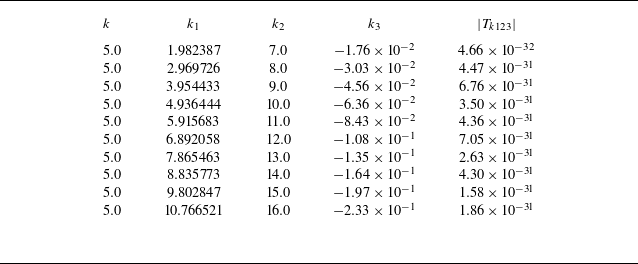
 Tk123
 β=0.001
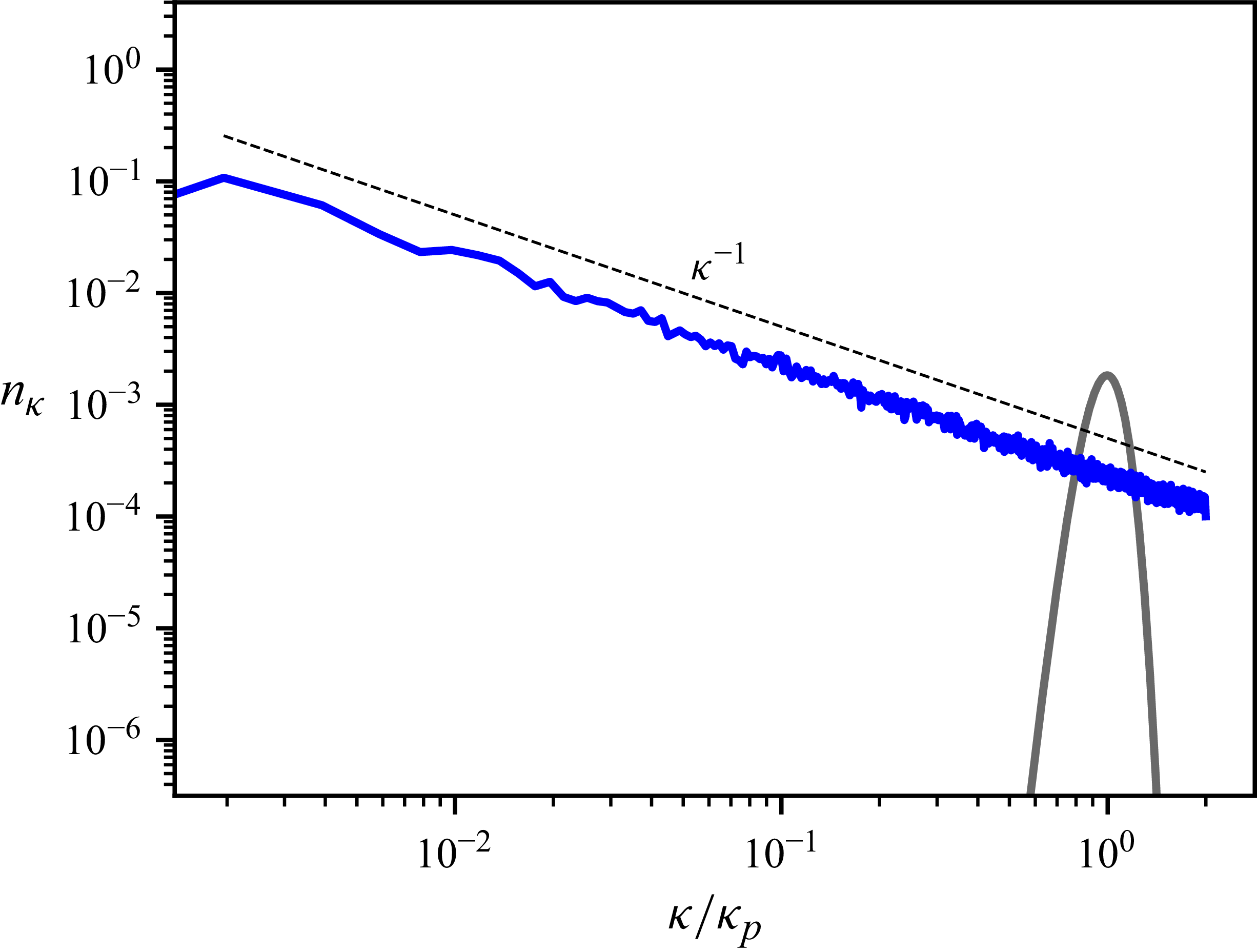
 t=0
 t=2×10⁶Tp
 α=β=0.2
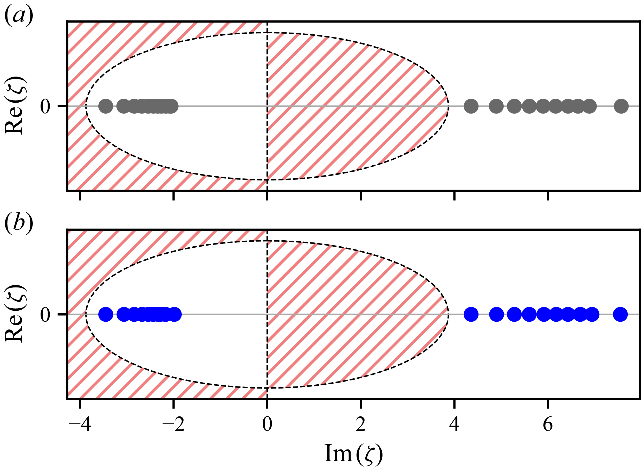
 ζ
 (a)
 t=0
 (b)
 t≈2×10⁶Tp
 E
 Im[E(ζ)]<0
 Im[E(ζ)]=0
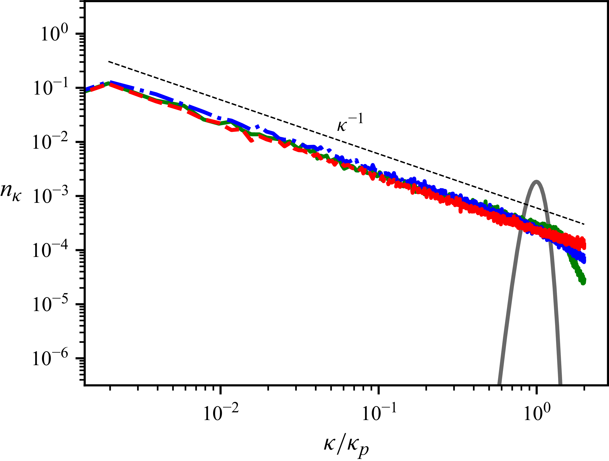
 α=0.2
 α=0.04
 α=0.02
 5×10⁵Tp
 8×10⁵Tp
 1.2×10⁶Tp

 B(κ,κ1)
 (a,c)
 α=0.2
 (b,d)
 α=0.02
 Δω=0.08
 α=0.2
 Δω=0.025
 α=0.02

 k
 ω
 Sη(k,ω)
 (a)
 α=0.2
 (b)
 α=0.02
 (a)
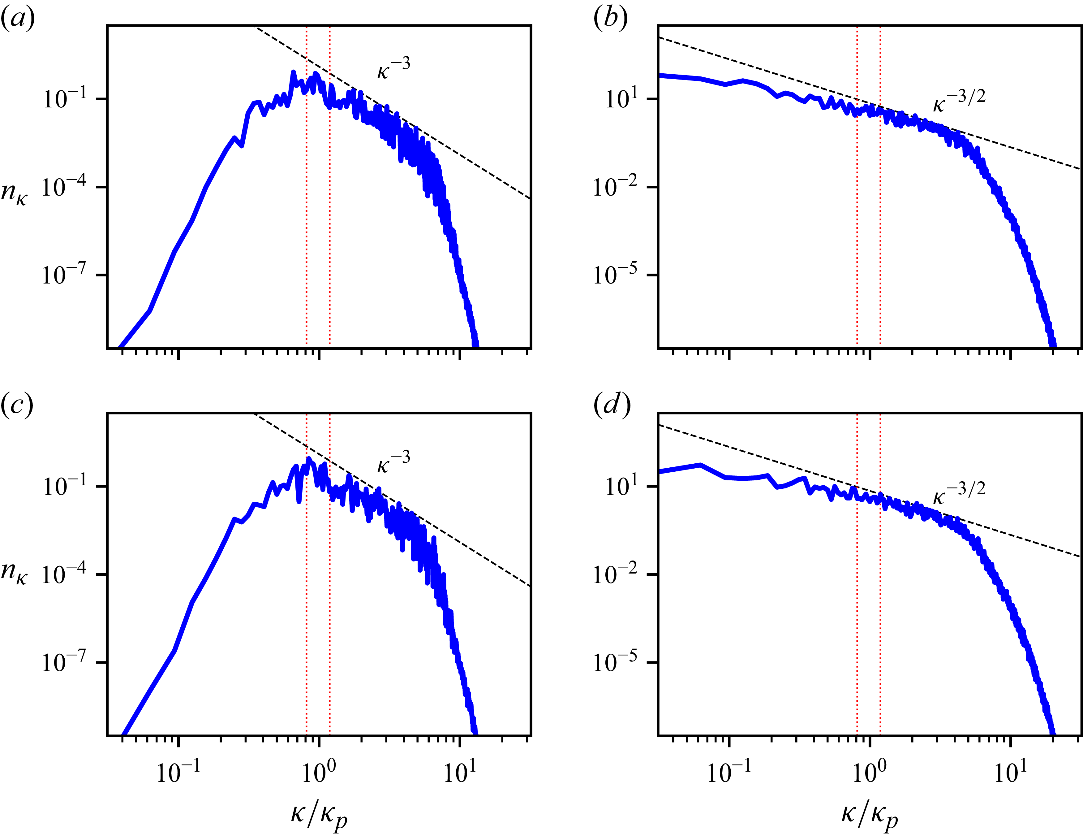
 (a,b)
 (c,d)
 nκ∼κ−3
 nκ∼κ−3/2

 Tk123
 β=0.001
 k=5.0
 |Δω|⩽2
 Δω=0
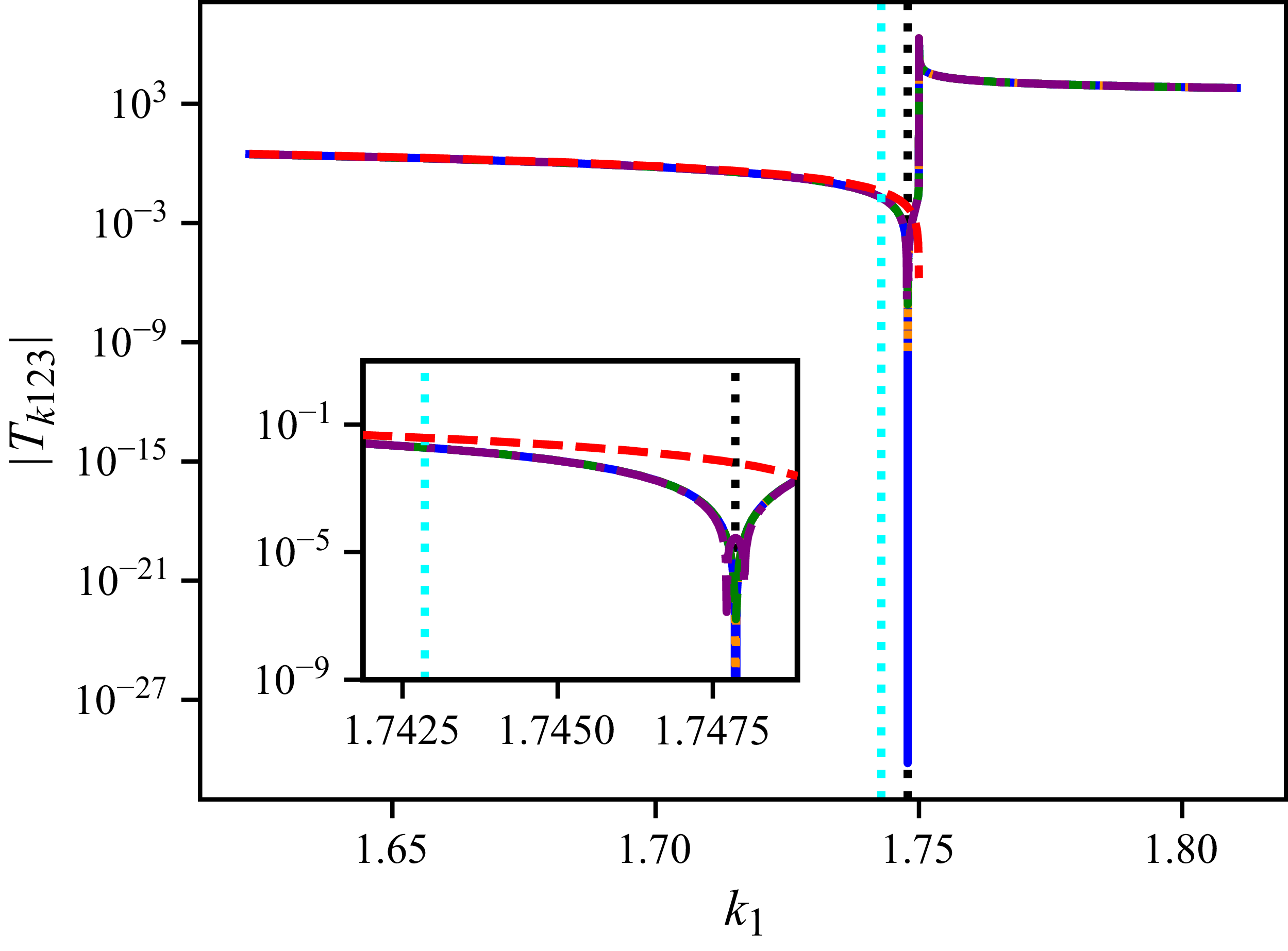
 Tk123
 β=0.001
 k=1.5
 k2=3.25
 O(β3)
 O(β2)
 O(β)
 |Δω|=0.01
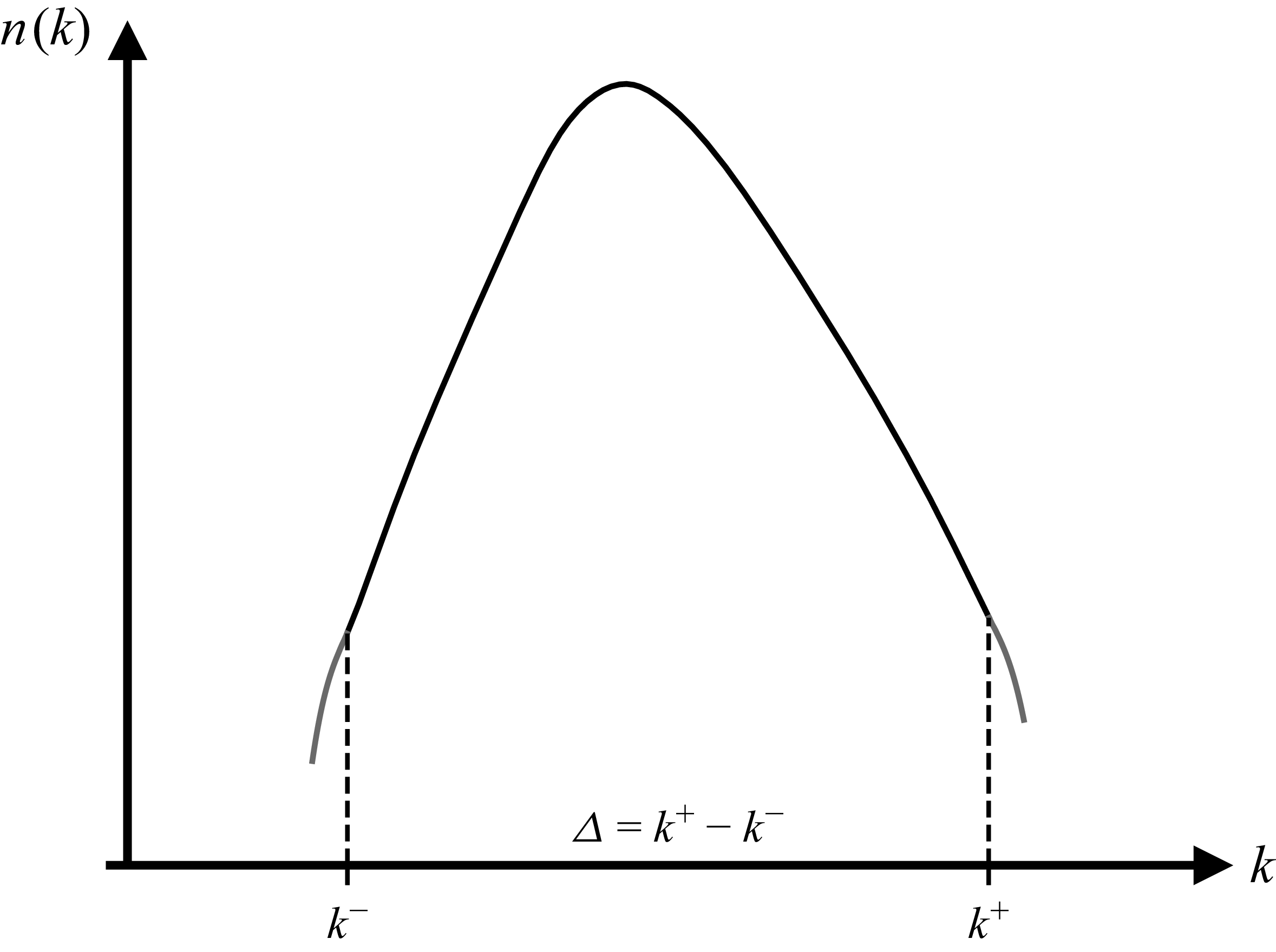
 Δ
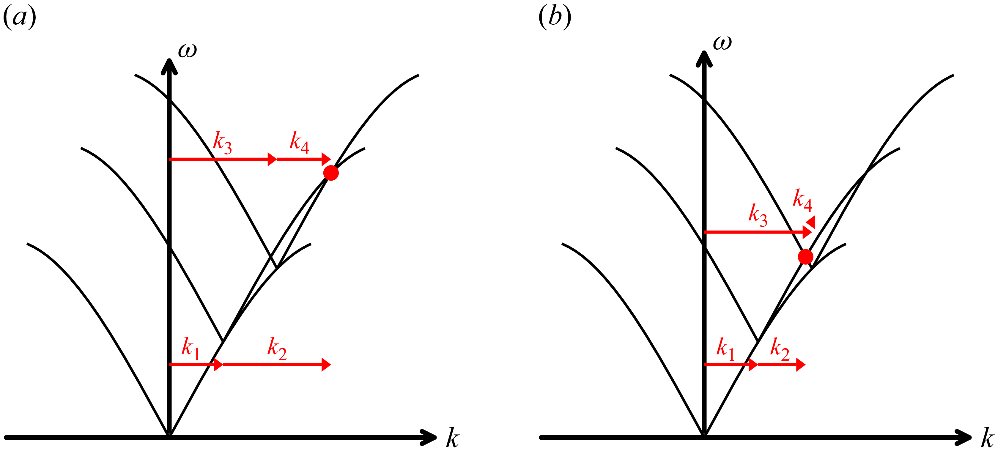
 (a)
 (b)
 k4
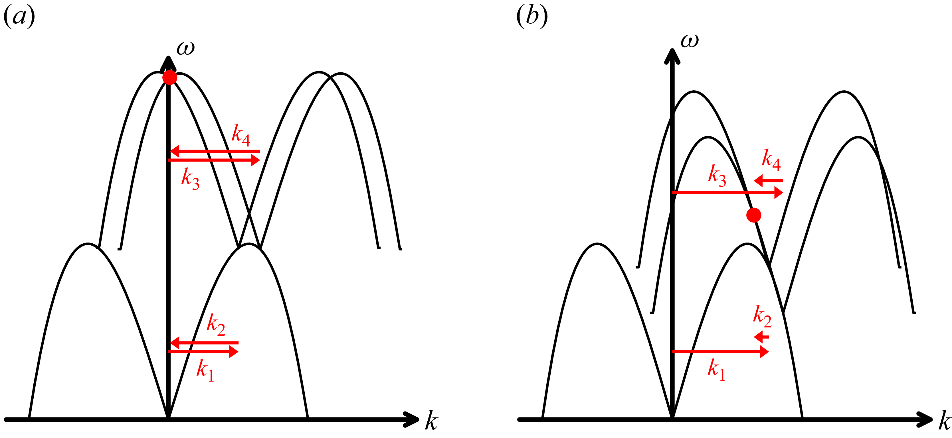
 (a)
 O(β−1/2)
 (b)
 O(1)
 O(β−1/2)

 (a)
 t=0
 t≈4×10⁵Tp
 α=β=4×10⁻⁵
 (b)
 k
 ω
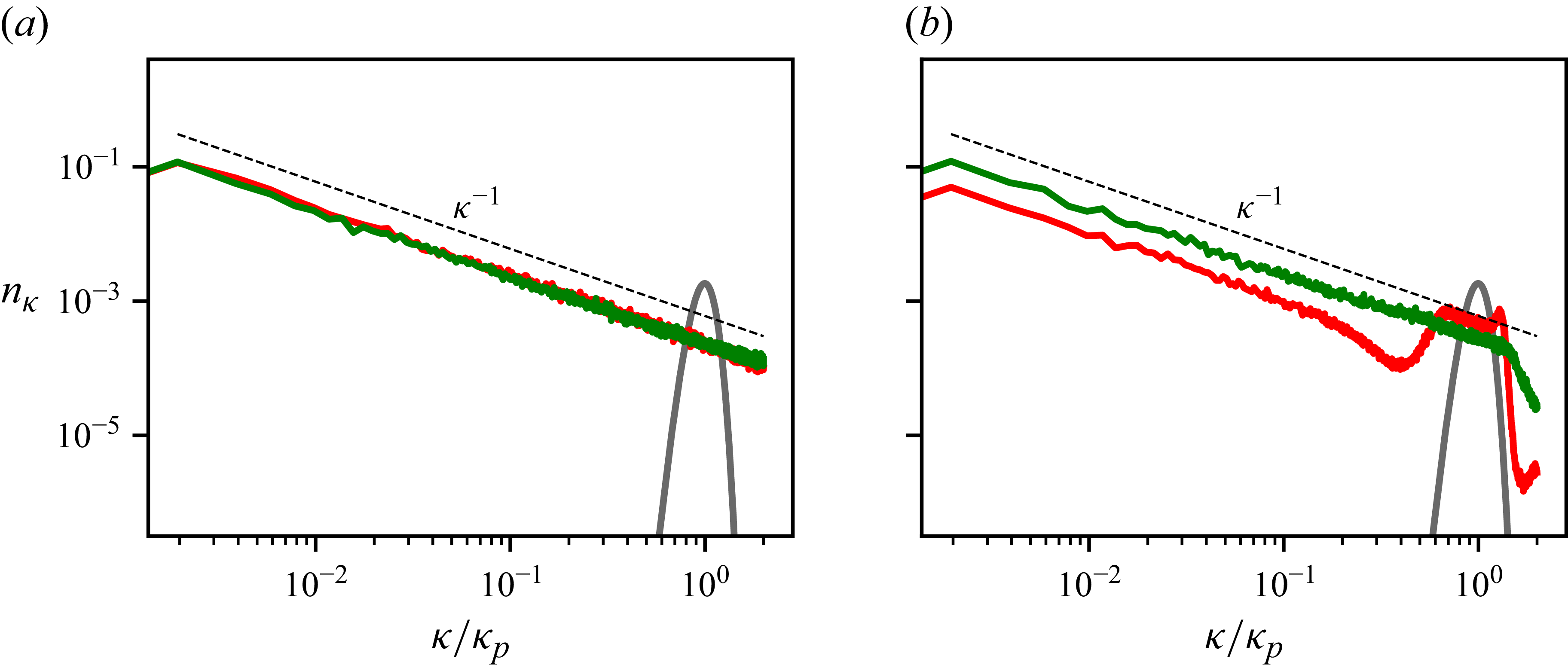
 nk∝|ηk|2/ωk
 (a)
 α=0.2
 5×10⁵Tp
 (b)
 α=0.02
 1.2×10⁶Tp
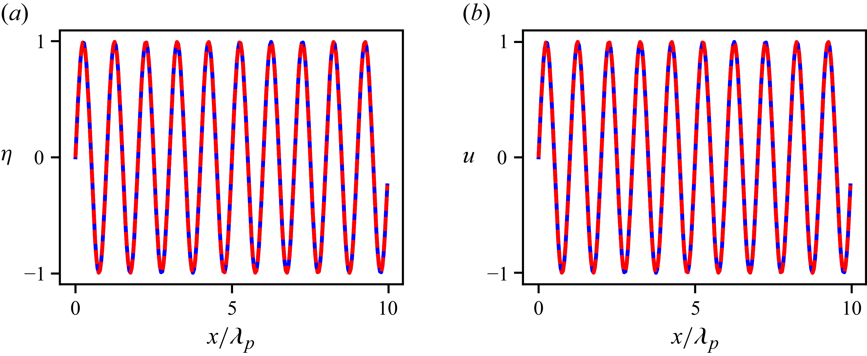
 (a)
 (b)
 t=10Tp
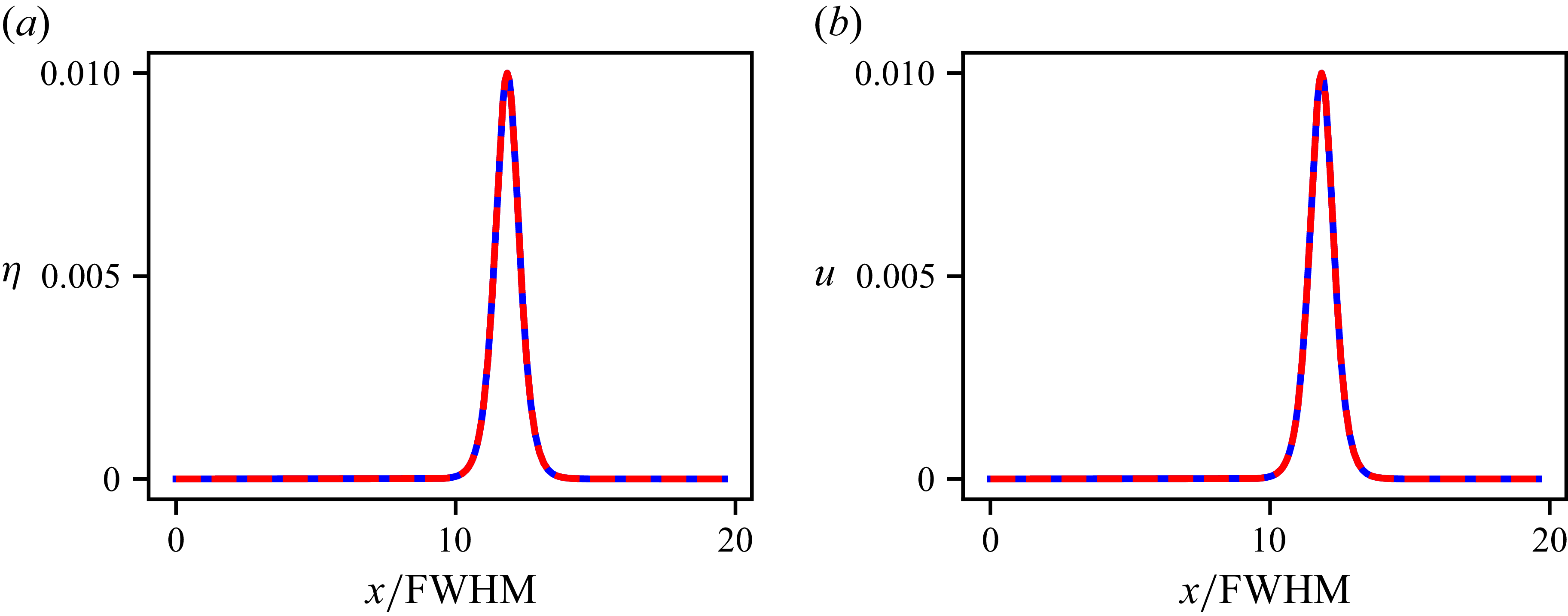
 (a)
 (b)
 t=2τs
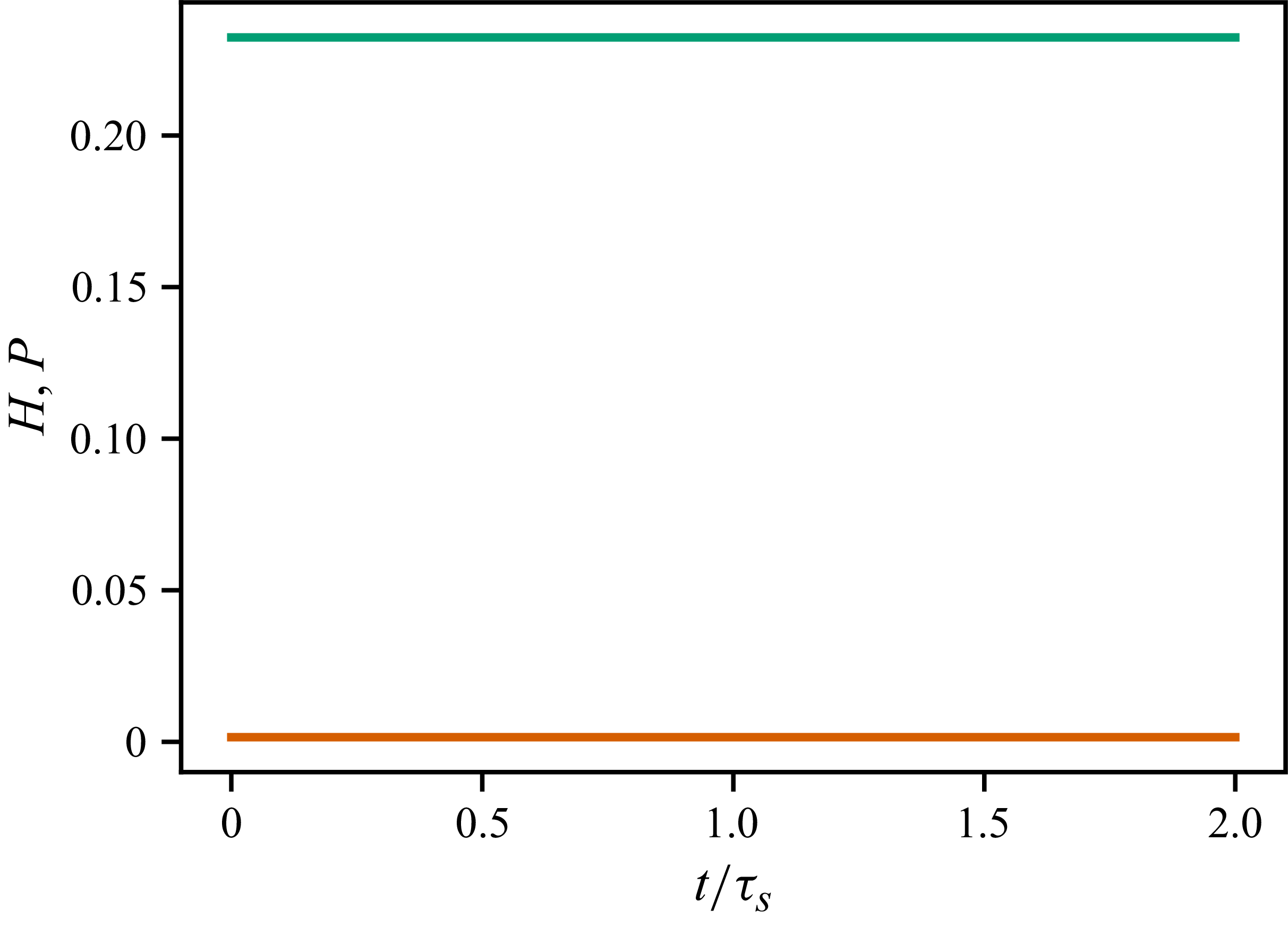
 P
 H
 2τs
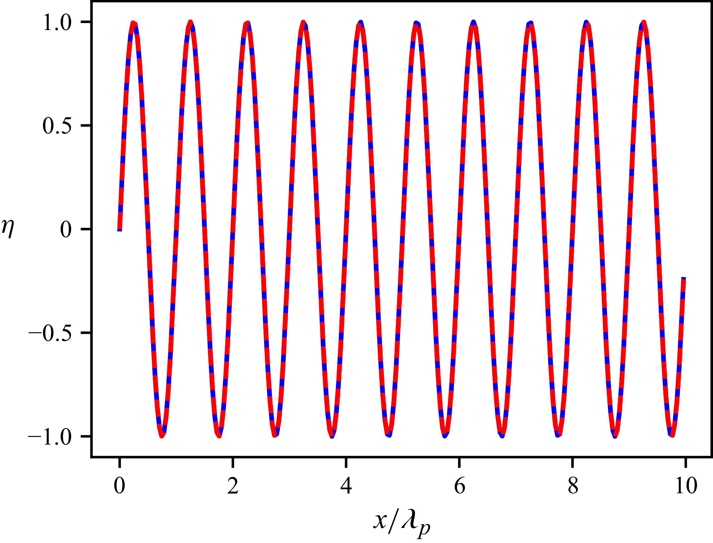
 t=10Tp
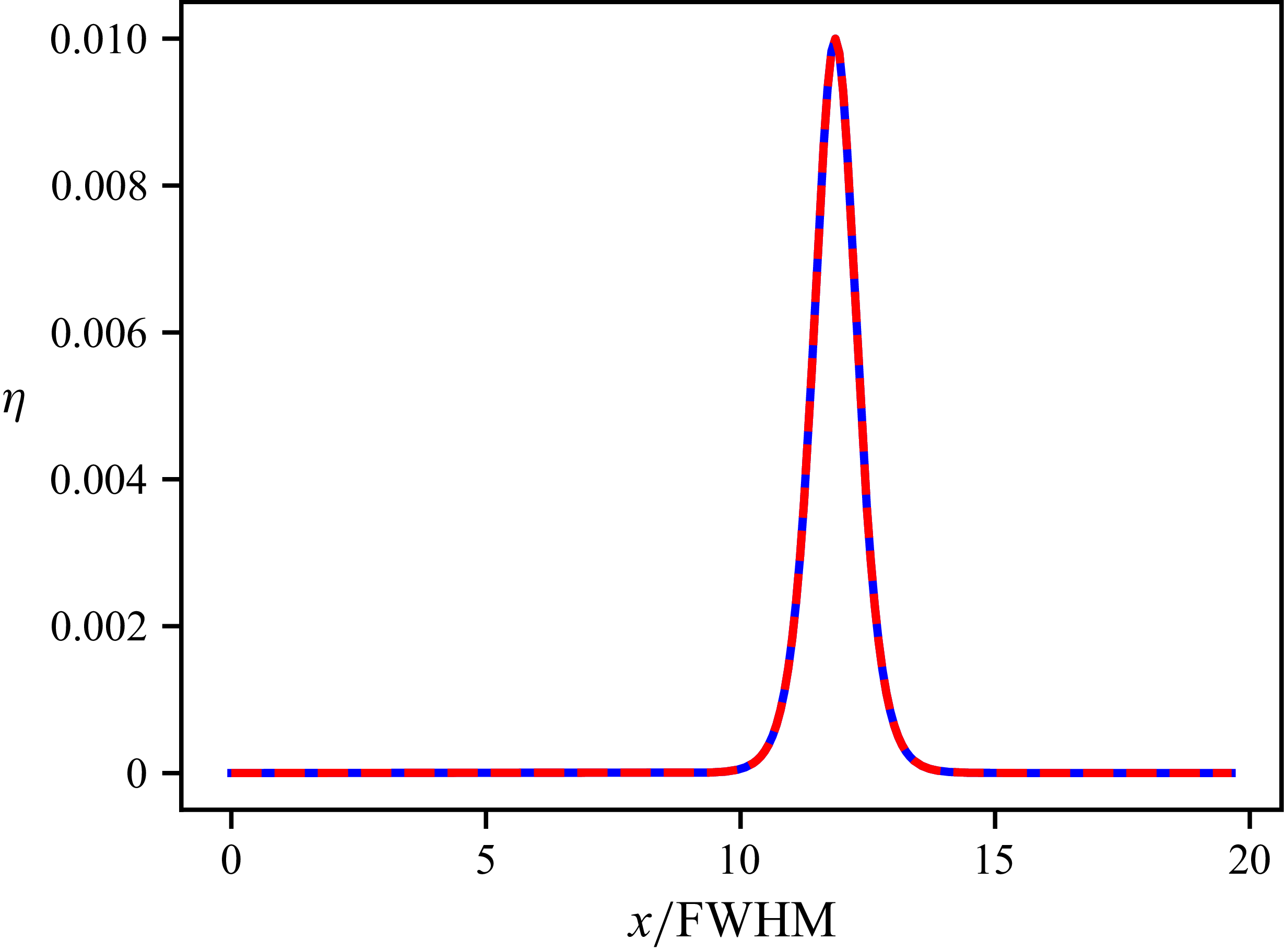
 t=2τs
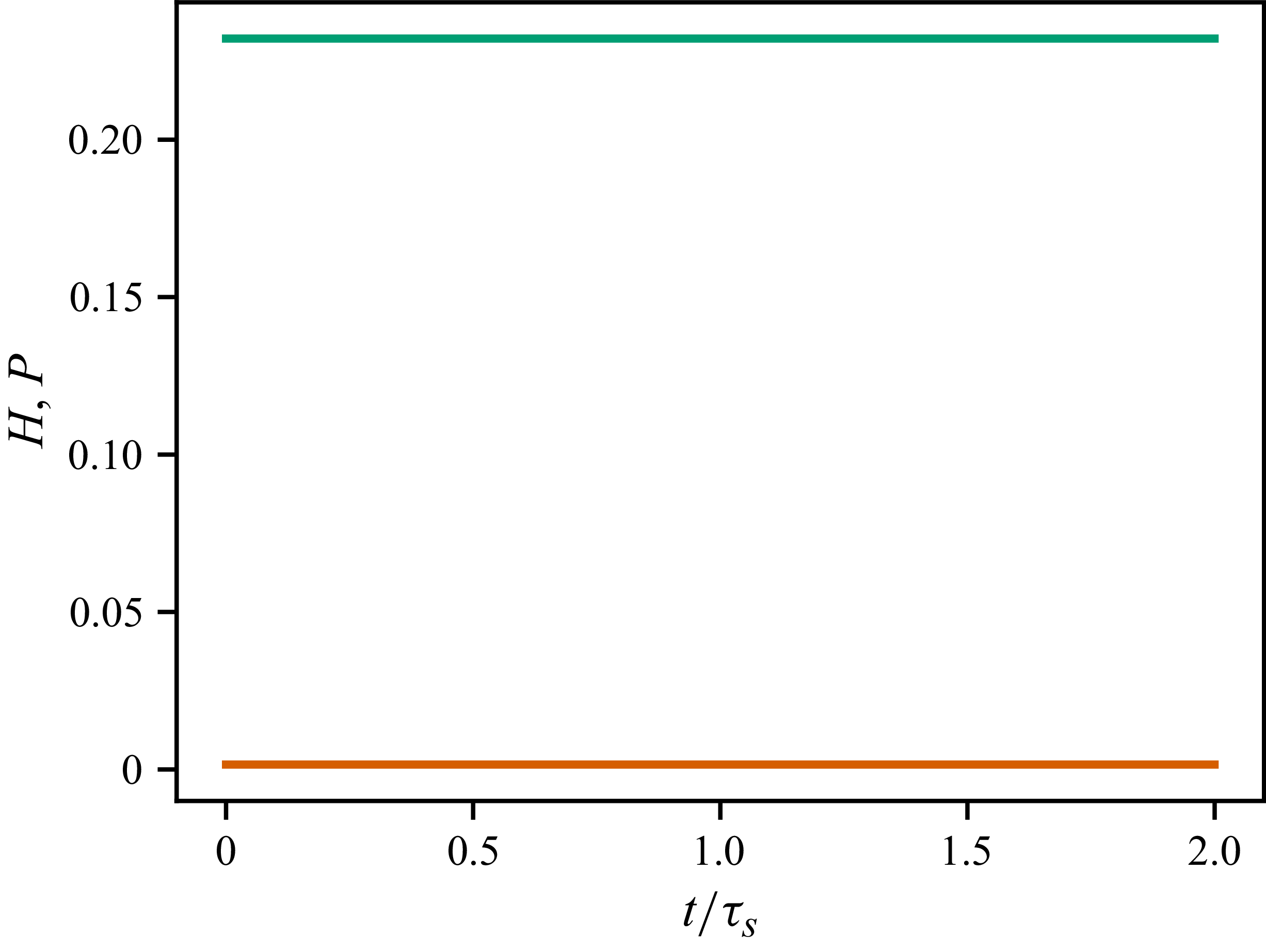
 P
 H
 2τs

 Open access

