2 The CBDX Model

Consider the following mortality model:

(1) \begin{align}\log m\!\left( {t,x} \right) = \alpha\!\left( x \right) + \mathop \sum \limits_{i = 1}^K {\beta _i}\!\left( x \right){\kappa _i}\!\left( t \right) + \gamma \!\left( c \right)\end{align}

where $m\!\left( {t,x} \right)$ is a death rate, t refers to the time period, x refers to age and $c = t - x$ refers to the year of birth. The $\alpha \!\left( x \right)$ , $\kappa \!\left( t \right)$ and $\gamma \!\left( c \right)$ are the age-related, period-related and cohort-related effects, and the parameters ${\beta _1} = 1$ , ${\beta _2} = \!\left( {x - \overline x } \right)$ and ${\beta _3} = {\!\left( {x - \overline x } \right)^2} - \sigma _x^2$ are fixed throughout, and where $\overline x $ and $\sigma _x^2$ are the mean and variance of the ages in our sample age range. As discussed next, this model is similar in spirit to Plat (Reference Plat2009) in adding an age effect, $\alpha \!\left( x \right)$ , to the original CBD models.

This model comes in three versions:

1. • $K = 1$ , that is, the case with only one $\kappa \!\left( t \right)$ variable - denoted model CBDX1.

2. • $K = 2$ , that is, the case with two $\kappa \!\left( t \right)$ variables - denoted model CBDX2.

3. • $K = 3$ , that is, the case with three $\kappa \!\left( t \right)$ variables - denoted model CBDX2.

This CBDX family of models is similar to the CBD family except for the following:

1. • It uses the log of the death rate, $\log m\!\left( {t,x} \right)$ , instead of the logit of the mortality rate, ${\rm{logit}}\;q\!\left( {t,x} \right)$ , as the dependent variable.

2. • It includes (as in Plat, Reference Plat2009) an additional age-related variable, $\alpha \!\left( x \right)$ .

3. • Whereas CBD model treats $\gamma \!\left( c \right)$ as a trendless mean-reverting AR(1) process, we treat $\gamma \!\left( c \right)$ as a residual that should be trendless and mean-reverting if the model is well specified.

4. • Model fitting differs from previous CBD family models by using a sequential maximum likelihood (ML) algorithm which is not dependent on any explicit identifiability constraints.Footnote ²

The Lee–Carter model showed the advantages of including a non-parametric “base mortality table”, $\alpha\!\left( x \right)$ , in equation (1). The advantages of our treatment of the $\gamma\!\!\left( c \right)$ process, of using a sequential algorithm, and of not relying on explicit identifiability constraints are discussed in the following.

3 The CBDX Model and Related Models

The CBDX model is related to a number of well-known mortality models, in particular Lee–Carter, M3, M5, M6, M7 and the Plat model.

The Lee–Carter model, referred to by Cairns et al. (Reference Cairns, Blake, Dowd, Coughlan, Epstein, Ong and Balevich2009) as M1, is

(2) \begin{align}\log m\!\left( {t,x} \right) = \alpha \!\left( x \right) + {\beta _2}\!\left( x \right){\kappa _2}\!\left( t \right)\end{align}

where $\alpha \!\left( x \right)$ is a non-parametric “base mortality table”, ${\beta _2}\!\left( x \right)$ is an age-dependent parameter and ${n_a}$ is the number of ages in the sample data age range. This model satisfies two identifiability conditions set out, for example, in Cairns et al. (Reference Cairns, Blake, Dowd, Coughlan, Epstein, Ong and Balevich2009: 7).

Model M3 (Cairns et al., Reference Cairns, Blake, Dowd, Coughlan, Epstein, Ong and Balevich2009) is the standard Age-Period-Cohort model, and is identical to what we label here as CBDX1, and so is not considered further.

Model M5 (Cairns et al., Reference Cairns, Blake, Dowd, Coughlan, Epstein, Ong and Balevich2009) is a reparameterised version of the CBD two-factor mortality model (Cairns et al., Reference Cairns, Blake and Dowd2006) and postulates that the mortality rate $q\!\left( {t,x} \right)$ satisfies

(3) \begin{align}{\rm{logit}}\;q\!\left( {t,x} \right) = {\kappa _1}\!\left( t \right) + \!\left( {x - \overline x } \right){\kappa _2}\!\left( t \right)\end{align}

where we assume that $q\!\left( {t,x} \right) = 1 - {{\rm{e}}^{ - m\!\left( {t,x} \right)}}$ , $\overline x $ is the average of the ages used in the sample age range and ${\boldsymbol\kappa _t} = \left[ {{\kappa _1}\!\left( t \right),{\kappa _2}\!\left( t \right)} \right]$ follows a two-dimensional random walk with drift:

(4) \begin{align}{\boldsymbol\kappa _t} = {\boldsymbol\kappa _{t - 1}} + \boldsymbol\mu + \textbf{\textit{C}}{Z_t}\end{align}

Model M5 does not have any identifiability issues.

Model M6 is a generalised version of M5 with a cohort effect:

(5) \begin{align}{\rm{logit}}\;q\!\left( {t,x} \right) = {\kappa _1}\!\left( t \right) + \!\left( {x - \overline x } \right){\kappa _2}\!\left( t \right) + \gamma \!\left( c \right)\end{align}

where the ${\boldsymbol\kappa _t}$ process follows (4) and $\gamma \!\left( c \right)$ is the cohort effect. This model satisfies the identifiability constraints:

(6) \begin{align}\mathop \sum \limits_{c = 1}^{{n_c}} \gamma \!\left( c \right) = 0 \quad \textrm{and} \quad\mathop \sum \limits_{c = 1}^{{n_c}} c\gamma \!\left( c \right) = 0\end{align}

where ${n_c}$ is the number of years of birth in the sample data.

Model M7 is a second generalised version of M5 with a cohort effect:

(7) \begin{align}{\rm{logit}}\;q\!\left( {t,x} \right) = {\kappa _1}\!\left( t \right) + \!\left( {x - \overline x } \right){\kappa _2}\!\left( t \right) + \left[ {{{\!\left( {x - \overline x } \right)}^2} - \sigma _x^2} \right]{\kappa _3}\!\left( t \right) + \gamma \!\left( c \right)\end{align}

where the period effects ${\boldsymbol\kappa _t}$ now follow a three-dimensional random walk with drift and $\gamma \!\left( c \right)$ is a cohort effect modelled as an AR(1) process. This model satisfies the identifiability constraints:

(8) \begin{align}\mathop \sum \limits_{c = 1}^{{n_c}} \gamma \!\left( c \right) = 0,\ \mathop \sum \limits_{c = 1}^{{n_c}} c\gamma \!\left( c \right) = 0 \quad \textrm{and} \quad \mathop \sum \limits_{c = 1}^{{n_c}} c^{2}\gamma \!\left( c \right) = 0 \end{align}

More details on the models can be found in Cairns et al. (Reference Cairns, Blake, Dowd, Coughlan, Epstein, Ong and Balevich2009).

CBDX2 and CBDX3 are similar to models M6 and M7, respectively, except in so far as they (a) use $\log m\!\left( {t,x} \right)$ rather than ${\rm{logit}}\;q\!\left( {t,x} \right)$ as the dependent variable; (b) include an additional age effect, $\alpha \!\left( x \right)$ ; (c) use a sequential estimation algorithm; and (d) (as a result of (c)) do not require any explicit identifiability constraints. CBDX2 is the same as the two period effect version of the Plat (Reference Plat2009) model and CBDX3 adds a third period effect to CBDX2.Footnote ³

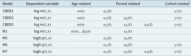
The age, period and cohort effects for the different models are summarised in Table 1.

Table 1.

Dependent variables and age-, period- and cohort-effects for different mortality models.

Note: $x$ = age, $t$ = period, $c$ = birth year.

It is also helpful to set out which models incorporate others as special cases of others. The two core special cases are M3 and M5. Ignoring differences in algorithms and identifiability conditions for present purposes:

1. • CBDX1 is a special case of CBDX2.

2. • CBDX2 is a special case of CBDX3.

3. • M5 is a special case of M6.

4. • M6 is a special case of M7.

4 Estimation of the CBDX Model

4.1. The sequential estimation algorithm

Let ${\rm{\Theta }} = \left\{ {\alpha ,\kappa ,\gamma } \right\}$ be the parameter set to be estimated, where $\kappa $ corresponds to ${\kappa _1}\!\left( t \right)$ for CBDX1, ( ${\kappa _1}\!\left( t \right),{\kappa _2}\!\left( t \right)$ ) for CBDX2 and ( ${\kappa _1}\!\left( t \right),{\kappa _2}\!\left( t \right),{\kappa _3}\!\left( t \right)$ ) for CBDX3, for $t = 1, \ldots ,\;{n_y}$ . The Poisson log-likelihood is then

(9) \begin{align} l\!\left( {\alpha ,\kappa ,\gamma } \right) &= \mathop \sum \limits_{t,x} \left[ {D\!\left( {t,x} \right)\log m\!\left( {t,x} \right) - E\!\left( {t,x} \right)m\!\left( {t,x} \right)} \right] + {{constant}}\; \nonumber\\ & = \mathop \sum \limits_{t,x} D\!\left( {t,x} \right)\!\left( {\alpha \!\left( x \right) + {\kappa _1}\!\left( t \right) + {\beta _2}\!\left( x \right){\kappa _2}\!\left( t \right) + {\beta _3}\!\left( x \right){\kappa _3}\!\left( t \right) + \gamma \!\left( {t - x} \right)} \right) \nonumber\\ &\qquad- \mathop \sum \limits_{t,x} E\!\left( {t,{x_j}} \right)\exp \!\left( \alpha \!\left( x \right) + {\kappa _1}\!\left( t \right) + {\beta _2}\!\left( x \right){\kappa _2}\!\left( t \right) + {\beta _3}\!\left( x \right){\kappa _3}\!\left( t \right) + \gamma \!\left( {t - x} \right) \right)\nonumber\\ &\qquad+ {constant} \end{align}

where ${\beta _2}\!\left( x \right) = \!\left( {x - \overline x } \right)$ and ${\beta _3}\!\left( x \right) = \left[ {{{\!\left( {x - \overline x } \right)}^2} - \sigma _x^2} \right]$ , $D\!\left( {t,x} \right)$ is the number of deaths in year t aged x last birthday, and $E\!\left( {t,x} \right)$ is the average number of individuals in year t aged x last birthday.

We propose the following sequential estimation algorithm.

4.1.1. Partial ML

Stage P1 (Alpha, Kappa) involves the joint estimation of the $\alpha \!\left( x \right)$ and $\kappa \!\left( t \right)$ parameters. Stage P2 (Gamma) uses $\widehat{\alpha } \!\left( x \right)$ and $\widehat{\kappa } \!\left( t \right)$ to estimate the $\gamma \!\left( c \right)$ parameters. This two-stage procedure is very much in the spirit of the GP of Hunt & Blake (Reference Hunt and Blake2014), in which the model structure identifies sufficient age and period effects first before adding a cohort effect to capture small residual patterns in the data by year of birth. At this point, Partial ML (PML) is complete. Although PML does not require any explicit identifiability constraints, they are implicit in the fact that the age and period effects are kept fixed while we estimate the cohort effects.

4.1.2. Full ML

We start with the three stages of PML. The Stage F1 (Alpha, Kappa) revision uses the latest $\widehat{\gamma} \!\left( c \right)$ to re-estimate the $\alpha \!\left( x \right)$ and $\kappa \!\left( t \right)$ . The Stage F2 (Gamma) revision then uses the latest $\widehat{\alpha } \!\left( x \right)$ and $\widehat{\kappa} \!\left( t \right)$ to re-estimate the $\gamma \!\left( c \right)$ state variables. We then repeat Stages F1 and F2 until all parameter estimates and the likelihood converge. These estimates are those that maximise the likelihood function.

4.2. Illustrating the sequential estimation algorithm using CBDX3

Consider CBDX3. In this case, $K = 3$ , ${\beta _1} = 1$ , ${\beta _2}\!\left( x \right) = \!\left( {x - \overline x } \right)$ and ${\beta _3}\!\left( x \right) = {\!\left( {x - \overline x } \right)^2} - \sigma _x^2$ , and (1) becomes the following:

(10) \begin{align}{\rm{log}}\;m\!\left( {t,x} \right) = \alpha \!\left( x \right) + {\kappa _1}\!\left( t \right) + \!\left( {x - \overline x } \right){\kappa _2}\!\left( t \right) + \left[ {{{\!\left( {x - \overline x } \right)}^2} - \sigma _x^2} \right]{\kappa _3}\!\left( t \right) + \gamma \!\left( c \right)\end{align}

4.2.1 Stage P1A (Alpha)

We now take (10) and set the $\kappa \!\left( t \right)$ and $\gamma \!\left( c \right)$ to zero to obtain

(11) \begin{align}log\;m\!\left( {t,x} \right) = \alpha \!\left( x \right)\end{align}

(12) \begin{align}m\!\left( {t,x} \right) = {{\rm{e}}^{\alpha \!\left( x \right)}}\end{align}

Implicitly, we are assuming that that the starting values of the $\kappa \!\left( t \right)$ and $\gamma \!\left( c \right)$ are zero for the purposes of estimating $\alpha \!\left( x \right)$ .

We then substitute (11) and (12) into (9) to obtain the log-likelihood function expressed in terms of $\alpha \!\left( x \right)$ :

(13) \begin{align}l\!\left( \alpha \right) = \mathop \sum \limits_{j = 1}^{{n_a}} \mathop \sum \limits_{t = 1}^{{n_y}} D\!\left( {t,{x_j}} \right)\alpha \!\left( {{x_j}} \right) - \mathop \sum \limits_{j = 1}^{{n_a}} \mathop \sum \limits_{t = 1}^{{n_y}} E\!\left( {t,{x_j}} \right){{\rm{e}}^{\alpha \!\left( {{x_j}} \right)}}\, + \,{{constatnt}}\end{align}

where ${n_y}$ is the number of sample years.

The ML estimator for $\alpha \!\left( {{x_i}} \right)$ is obtained by differentiating (13) with respect to $\alpha \!\left( {{x_j}} \right)$ and rearranging the first-order condition to give

(14) \begin{align}\widehat{\alpha} \!\left( {{x_j}} \right) = {\rm{log}}\left\{ {\frac{{\mathop \sum \nolimits_{t = 1}^{{n_y}} D\!\left( {t,{x_j}} \right)}}{{\mathop \sum \nolimits_{t = 1}^{{n_y}} E\!\left( {t,{x_j}} \right)}}} \right\}\end{align}

for $j = 1, \ldots ,{n_a}$ .

4.2.2 Stage P1K (Kappa)

In this stage, we input the estimate $\widehat{\alpha} \!\left( x\right)$ obtained from Stage P1A into (10):

(15) \begin{equation}{\rm log}\ m\!\left(t,x\right)=\widehat{\alpha }\!\left(x\right)+{\kappa }_1\!\left(t\right)+(x-\overline{x}){\kappa }_2\!\left(t\right){+[{(x-\overline{x})}^2-{\sigma }^2_x]\kappa }_3\!\left(t\right)\end{equation}

We then obtain the log-likelihood function

(16) \begin{align} &l\!\left( {{\kappa _1},{\kappa _2},{\kappa _3}} \right)\nonumber \\ & = \sum^{n_y}_{t=1}{\sum^{n_a}_{j=1}{ \begin{array}{c}D\!\left(t,x_j\right)\!\left(\widehat{\alpha }\!\left(x_j\right)+{\kappa }_1\!\left(t\right)+\!\left(x_j-\overline{x}\right){\kappa }_2\!\left(t\right){+\left[{\!\left(x_j-\overline{x}\right)}^2-{\sigma }^2_x\right]\kappa_3}\!\left(t\right)\right) \end{array}}} \nonumber \\ &\quad - \sum^{n_y}_{t=1}{\sum^{n_a}_{j=1}{E\!\left(t,x_j\right)e^{\widehat{\alpha }\!\left(x_j\right)}e^{{\kappa }_1\!\left(t\right)}e^{(x_j-\overline{x}){\kappa }_2\!\left(t\right)}}e^{{[{(x_j-\overline{x})}^2-{\sigma }^2_x]\kappa }_3\!\left(t\right)}}+ constant \end{align}

We obtain estimates of ${\kappa _1}\!\left( t \right)$ , ${\kappa _2}\!\left( t \right)$ and ${\kappa _3}\!\left( t \right)$ that maximise (16) using a Newton-Raphson iterative algorithm.

4.2.3 Stage P1C

Repeat stages P1A and P1K until the estimates and the log-likelihood have converged.

4.2.4 Stage P2G (Gamma)

In this stage, we input the estimates $\widehat{\alpha}(x),\ \widehat{\kappa}_{1}(t),\ \widehat{\kappa}_{2}(t)$ and $\ {\widehat{\kappa}_3}(t)$ into (10) to obtain

(17) \begin{equation}{\rm log}\ m\!\left(t,x\right)=\widehat{\alpha }\!\left(x\right)+{\widehat{\kappa }}_1(t)+\!\left(x-\overline{x}\right){\widehat{\kappa }}_2(t)+[{\!\left(x-\overline{x}\right)}^2-{\sigma }^2_x]{\widehat{\kappa }}_3\!\left(t\right)+\gamma (c)\end{equation}

We then derive the log-likelihood function in terms of $\gamma :$

(18) \begin{align}& l\!\left( \gamma \right) \nonumber \\ & \quad = \sum^{n_y}_{t=1}{\sum^{n_a}_{j=1}{D\!\left(t,x_j\right)\!\left(\widehat{\alpha }\!\left(x_j\right)+{\widehat{\kappa }}_1\!\left(t\right)+(x_j-\overline{x}){\widehat{\kappa }}_2\!\left(t\right)+\left[{\!\left(x_j-\overline{x}\right)}^2-{\sigma }^2_x\right]{\widehat{\kappa }}_3\!\left(t\right)+\gamma \!\left({t-x}_j\right)\right)}}\nonumber\\ &\qquad -\sum^{n_y}_{t=1}{\sum^{n_a}_{j=1}{E\!\left(t,x_j\right)e^{\widehat{\alpha }\!\left(x_j\right)}e^{{\widehat{\kappa }}_1\!\left(t\right)}e^{(x_j-\overline{x}){\widehat{\kappa }}_2\!\left(t\right)}{e^{[{\!\left(x_j-\overline{x}\right)}^2-{\sigma }^2_x]{\widehat{\kappa }}_3\!\left(t\right)}e}^{\gamma ({t-x}_j)}}}+ {constant} \end{align}

We then differentiate the log-likelihood function (18) with respect to $\gamma \!\left( c \right)$ and rearrange the first-order conditions to obtain the ML estimate (MLE) for $\gamma \!\left( c \right)$ :

(19) \begin{equation}\hat\gamma \!\left(c\right)=log\left\{\frac{\sum^{n_y}_{t=1}{\sum^{n_a}_{j=1}{w_c\!\left(t,x_j\right)D\!\left(t,x_j\right)}}}{\sum^{n_y}_{t=1}{\sum^{n_a}_{j=1}{w_c\!\left(t,x_j\right)E\!\left(t,x_j\right)e^{\widehat{\alpha}\!\left(x_j\right)}e^{{\widehat{\kappa }}_1\!\left(t\right)}e^{(x_j-\overline{x}){\widehat{\kappa }}_2\!\left(t\right)}e^{\left[{\!\left(x_j-\overline{x}\right)}^2-{\sigma }^2_x\right]{\widehat{\kappa }}_3\!\left(t\right)}}}}\right\}\end{equation}

for $\;c = 1, \ldots ,{n_c}$ , and where the weighting function ${w_c}\!\left( {t,x} \right)$ satisfies

(20) \begin{equation}{w_c}\!\left( {t,x} \right) = \left\{ {\begin{array}{c}1\\0\end{array}} \right\}\ \textrm{if}\ \left\{\begin{array}{l}t-x=c\\ t-x\neq c\end{array}\right.\end{equation}

4.2.5 Full maximum likelihood

As explained under Section 4.1.2.

5 Data and Results from Estimating the Model

5.2. Results

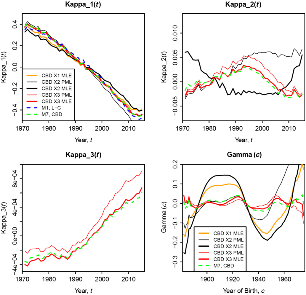
We compare results for the following models: Lee–Carter (M1, full MLE), the original CBD model (M5, MLE), second-generation CBD models M6 and M7 (MLE), and CBDX1, CBDX2 and CBDX3 (both PML and MLE in each case). Figure 1 compares fitting results for a selection of these models for the fitted period and cohort effects.

Figure 1

Estimated period and cohort effects for selected models.

For these selected models, we see that estimates for ${\kappa _1}\!\left( t \right)$ are quite consistent (top left panel)Footnote ⁴ reinforcing the notion that ${\kappa _1}\!\left( t \right)$ captures the headline mortality improvements at all levels. There is a close correspondence between M7 and CBDX3 (PML and MLE) in all four plots indicating that there is robustness in the addition of $\alpha \!\left( x \right)$ and in the switch from ${\rm{logit}}\;q\!\left( {t,x} \right)$ to $\log m\!\left( {t,x} \right)$ as the dependent variable. On the other hand, differences in the fitted cohort effects between the six models plotted are quite striking. Specifically, cohort effects for CBDX1 and CBDX2 (MLE) are much larger and have much more structure than for M7 and CBDX3, while for CBDX2, the PML and MLE cohort effects are quite different, indicating a lack of robustness.

This is a clear indication that CBDX1 and CBDX2 lack sufficient structure in the main age and period effects and that the cohort effect is being used as a proxy for capturing unmodelled age or period effects. This point can be seen by comparing the results for CBDX2 for the PML and MLE cases. The PML fits the age and period effects first, and the cohort effect second. As a rule of thumb, residuals by year of birth for the age-period case should approximately match the fitted cohort in the MLE. However, this is not the case for CBDX2, and is a further indication that, for this data set, the age and period effects in CBDX2 lack sufficient structure.

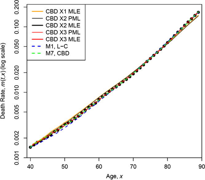
In Figure 2, as a snapshot of how well the models fit the data, we show actual death rates (dots) versus fitted death rates for various models. We can see that all of the models shown give a reasonable fit, but some models clearly fit much more closely than others. Models that fit less well are M1, CBDX1-MLE and CBDX2-PML, while the others are much closer and difficult to distinguish. Again, we see a significant difference between CBDX2-PML and CBDX2-MLE, indicating that the two age-period effects are not sufficient to capture the dynamics over the 45-year period. In contrast, the difference between CBDX3-PML and CBDX3-MLE is negligible.

Figure 2

Crude and fitted death rates in 2015 for selected models.

6 BIC Model Comparisons

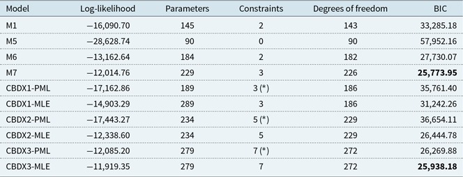
To assess how well the models compare, Table 2 shows the BIC results for M1, M5, M6, M7, and CBDX1, CBDX2 and CBDX3 under their PML and MLE variants.Footnote ⁵

Table 2.

Log-likelihoods and BIC results.

Note: Constraints marked with a (^*) are implicit rather than explicitly applied in the model-fitting process.

Table 3.

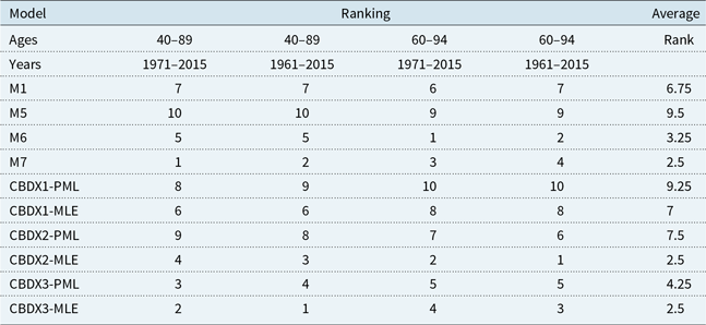
BIC-based model rankings for alternative age ranges and ranges of years.

Based on the BIC results, M7 should be marginally preferred to CBDX3. We also note that M1 and M5 both perform relatively poorly, presumably because of their simple structure and their lack of a cohort effect. In addition, we see that there is a substantial difference between the CBDX2 PML and MLE variants.

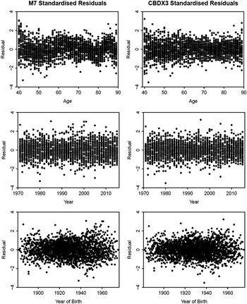
Figure 3 presents Pearson standardised residuals for M7 and CBDX3. These are quite similar across the models. However, M7 residuals by age (top left panel) exhibit a modest wave pattern that CBDX3 eliminates through its use of its additional age effect, $\alpha \!\left( x \right)$ . Otherwise, the plots in Figure 3 indicate that both models fit the data very well. But the top left panel does suggest that CBDX3 might be preferred over M7, notwithstanding the BIC scores.

The results reported above are based on sample age range of 40–89 and years 1971–2015. As a robustness check, Table 3 reports the BIC rankings for a variety of age ranges and years.

We see that models M7, CBDX2-MLE and CBDX3-MLE consistently perform well across different sample age and year ranges and generate the same average ranks.

We also see that the best performing models on the wider age ranges (see first two columns) are M7 and CBDX3-MLE: they both rank 1 or 2. From these results, there is nothing to choose between them. But then introduce the scatter plots in Figure 3 and the balance swings in favour of CBDX3-MLE. We would therefore argue that the best performing model on the wider age range is CBDX3-MLE.

Figure 3

Scatter plots of Pearson standardised residuals for M7 and CBDX3 against age (top), calendar year (middle) and year of birth (bottom).

On the other hand, if one wants to use a narrower (i.e., older) age range (see the third and fourth columns), then the two equal best performers are M6 and CBDX2-MLE and there is nothing to choose between them either.

Finally, we also observe that the PML versions of the CBDX models always rank worse than their MLE counterparts, and the difference in ranking is especially marked for CBDX1 and CBDX2.

7 A Financial Application

We now consider a financial application of the models which focus on annuity prices for two cohorts of males: one aged exactly 70, and one aged 50 at the start of 2016.

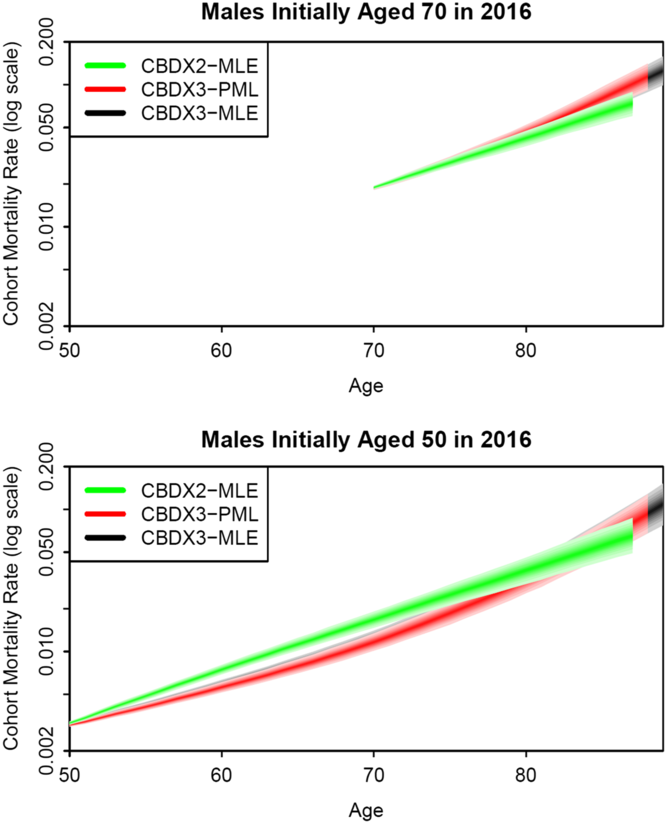
Figure 4 shows fan charts (covering the 5% to the 95% quantiles) of the underlying death rates for the two cohorts up to age 89. In both plots, the two variants of CBDX3 give quite consistent results due to the similarity of the historical period and cohort effects. CBDX2 initially tracks CBDX3-MLE fairly closely in the upper plot, but then deviates quite significantly. In the lower plot, CBDX2-MLE follows quite a different path. There are three reasons for these differences. First, the single values of the cohort effects for these cohorts (born in 1946 and 1966, respectively) are quite different (Figure 1, bottom right panel). Second, the upwards drift in ${\kappa _3}\!\left( t \right)$ (Figure 1, bottom left panel; an effect not present in CBDX2) causes mortality rates at high ages to improve at a slower rate in CBDX3. Third, in Figure 4, we can see that fitted death rates in 2015 are higher for CBDX2-MLE than either CBDX3 over the ages 50–70.

Figure 4

Fan charts for CBDX3-PML and CBDX3- MLE and CBDX2-MLE cohort $q$ rates.

Note: Based on E&W data for years 1971–2015 and ages 40–89.

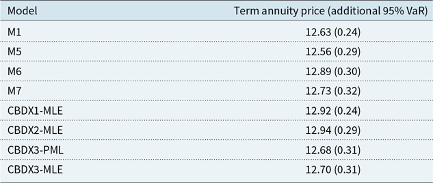
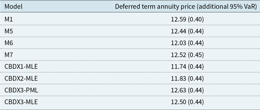
Tables 4 and 5 show the prices, per £1 per annum, of term annuities payable to males aged exactly 70 and 50, respectively. For the 70-year-old, payments commence immediately and are payable until age 90, and for the 50-year-old, the annuity is deferred to age 65 and ceases at age 90. For the 70-year-old, we can see some variation in prices, with M6, CBDX1 and CBDX2 well above the other models. This can be attributed to the significant differences in the fitted cohort effect at age 70 (year of birth 1946 in Figure 1, bottom right panel). For the 50-year-old, price differences between models are reversed and again mainly reflect differences in the fitted cohort effects for year of birth 1966. These differences emphasise the importance of (a) getting a good estimate of the cohort effect and (b) ensuring that the model has adequate age and period effects to avoid overfitting with the cohort effect. Figure 4 also helps to illustrate how these price differences emerge in relation to differences in the underlying mortality rates. For example, for the cohort aged 50, the higher mortality rates up to age 80 in the CBDX2 fan lead to lower survival probabilities and lower deferred annuity values.

Table 4.

Prices of a term annuity function from age 70.

Note: Based on E&W data for years 1971–2015 and ages 40–89. The term annuity presumes a continuously compounding risk-free interest rate of 1.5% p.a.

Table 5.

Prices of a deferred term annuity function from age 50 with payments commencing at age 65.

Note: Based on E&W data for years 1971–2015 and ages 40–89. The deferred term annuity presumes a continuously compounding risk-free interest rate of 1.5% p.a.

Tables 4 and 5 also include in parentheses the additional capital required to cover run-off of the liability at a 95% level of confidence (additional 95% value-at-risk (VaR)).Footnote ⁶ Models M1 and CBDX1 have less uncertainty in simulated mortality rates at high ages than other models, and this results in lower VaRs for these models. Other models have similar VaR levels. At age 70, VaRs are larger than the variation in prices between models. At age 50, VaRs are much higher as payments are more distant and more risky. We also see that variations in prices are larger than the VaRs.

8 Recalibrating Forecasts

In this section, we propose a novel method for forecasting that blends statistical analysis of the historical period effects with expert judgment (EJ) about central forecasts.

Current practice in the UK life insurance industry following guidance from the UK’s Prudential Regulation Authority (PRA, 2016) can be summarised as follows. Establish a best estimate (BE) for future mortality using, for example, EJ or statistical modelling. As a separate exercise, identify distinct stochastic mortality models from four common families of model (e.g., CBD, Lee–Carter) calibrated using standard statistical methods for their volatilities. For each model, calculate BE annuity liabilities and the associated solvency capital requirement (SCR) as a percentage of the same model’s BE. Use EJ to establish a single percentage SCR based on results for the four models. Finally, apply this percentage SCR to the BE-EJ best estimate based on EJ. While this approach on the face of it seems reasonable, there is an uncomfortable disconnect between the model used to establish the BE, and the models used to establish how much uncertainty there is around that BE. The approach we propose here resolves this issue.

Our new model for forecasting the period effects is generalised to a multivariate random walk with time-dependent drifts:

(21a) \begin{align}{K_1}\!\left( t \right) = {K_1}\!\left( {t - 1} \right)+ \mu_{1}(t)+{Z_1}\!\left( t \right)\end{align}

(21b) \begin{align}{K_2}\!\left( t \right) = {K_2}\!\left( {t - 2} \right)+ \mu_{2}(t)+{Z_2}\!\left( t \right)\end{align}

(21c) \begin{align}{K_3}\!\left( t \right) = {K_3}\!\left( {t - 3} \right)+ \mu_{3}(t)+{Z_3}\!\left( t \right)\end{align}

where $({Z_1}( t ),{Z_2}( t ),{Z_3}( t ))$ are independently identically distributed (i.i.d.) multivariate normal vectors with mean 0 and $Cov({Z_i}( t ),{Z_j}( t )) = {\sigma _{ij}}$ are estimates from the historical observations of $({K_1}( t ),\;{K_2}( t ),{K_3}( t ))$ .

The standard model has ${\mu _j}\!\left( t \right) = {\mu _j}$ , that is, constant drift, estimated from the historical data:

(22) \begin{align} \widehat{\mu}_{j}=({K_j}\!\left( {{t_1}} \right) - {K_j}\!\left( {{t_0}} \right)/\!\left( {{t_1} - {t_0}} \right)\end{align}

The proposed model assumes

(23) \begin{align}{\mu _j}\!\left( t \right) = \!\left( {{\mu _{j0}} - {\mu _{j1}}} \right){{\rm{e}}^{ - \beta \!\left( {t - {t_1}} \right)}} + {\mu _{j1}}\end{align}

So for each ${K_j}\!\left( t \right),$ we require

1. (a) ${K_j}\!\left( {{t_1}} \right)\,{=}\,$ last observation (already known),

2. (b) ${\mu _{j0}}\,{=}\,$ short-term drift,

3. (c) ${\mu _{j1}}\,{=}\,$ long-term drift and

4. (d) $\beta \,{=}\,$ rate at which we move from ${\mu _{j0}}$ to ${\mu _{j1}}$

with (b), (c) and (d) to be specified by the user. Other models for ${\mu _j}\!\left( t \right)$ are, of course, possible (e.g., as in CMI, 2018).

One procedure for calibration is to (1) choose ${\mu _{j0}} = $ an estimate of the recent trend in ${K_j}\!\left( t \right)$ up to ${t_1}$ ; (2) calibrate $\!\left( {{\mu _{11}},{\mu _{21}},{\mu _{31}}} \right)\kern-1.5pt,$ so that the prices of three annuities for ages 60, 65 and 70 match stated prices (BE liabilities) ${P_{60}}$ , ${P_{65}}$ and ${P_{70}}$ that might have been established using a given BE projection of mortality, for example, using the CMI mortality projections model (CMI, 2018).Footnote ⁷

By calibrating the ${\mu _{jk}}$ in this way, we have a single stochastic model that matches BE liabilities (e.g., as output from a different model such as CMI (2018), calibrated using EJ) and gives us a consistent estimate of the uncertainty around that liability. Having a single model that delivers both characteristics within a coherent setting gives us more confidence that the value-at-risk associated with the BE is reliable.

By way of example, we considered two variants alongside the baseline documented in the previous section:

1. • Variant 1: ${\mu _0}\,{=}\,$ mean drift (vector) over the period 2011–2015; ${\mu _1}\,{=}\,$ long-term historical drift (1971–2015).

2. • Variant 2: ${\mu _0}\,{=}\,$ mean drift (vector) over the period 2011–2015; ${\mu _1}\,{=}\,$ (0.015,0,0) (i.e., in the long run, the improvement rate will be 1.5% per annum at all ages from 50 to 89, consistent with recent actuarial practice).

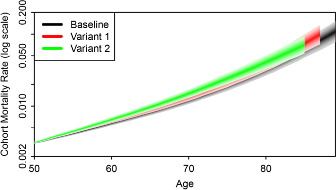
Table 6 gives prices and VaRs for the deferred annuity from age 50, and the immediate annuity from age 70, while Figure 5 shows fan charts for the cohort mortality rates from age 50 for the three variants.

Table 6.

Deferred and immediate annuity prices for three calibrations of the time-dependent drift of the multivariate random walk.

Figure 5

Cohort mortality fan charts for three variants with different parameters for the random walk drifts: males aged 50 in 2016.

Figure 5 helps to illustrate how differences in prices emerge under the three variants. Variant 1 deviates initially from the baseline because of the lower initial improvement rate, but, thereafter, tracks the trend of the baseline fan. The overall higher mortality then results in a lower price in Table 6. Variant 2 tracks Variant 1 initially, having the same initial rate of improvement, but then deviates from Variant 2 because of the different long-term improvement rates.

9 Features and Extensions of the CBDX Model