1. Introduction
Complex fluids come in tremendous variety – particulate and polymer suspensions, polymer melts, liquid crystalline and liquid crystal polymer fluids, flexible fibre suspensions and ‘active’ bacterial baths, to name only a few. While it is very challenging to understand any of these systems, it is especially challenging when the microstructure of a suspension has many degrees of freedom, such as flexible fibres that can assume complex shapes through flow-induced bending and buckling. As a fluid–structure problem, the interaction of flexible fibres with flows is very common, arising in micro-organismal and mucal transport by flagella or cilia (Gray Reference Gray2001), in determining the shape of biofilm streamers (Rusconi et al. Reference Rusconi, Lecuyer, Guglielmini and Stone2010, Reference Rusconi, Lecuyer, Autrusson, Guglielmini and Stone2011), in the abrupt appearance of normal stress differences (Goto, Nagazono & Kato Reference Goto, Nagazono and Kato1986; Zirnsak, Hur & Boger Reference Zirnsak, Hur and Boger1994) observed in wood pulp suspensions in the paper processing industry and in microfluidic engineering where flow control using flexible particles has recently been explored (Attia et al. Reference Attia, Pregibon, Doyle, Viovy and Bartolo2009; Wexler et al. Reference Wexler, Trinh, Berthet, Quennouz, du Roure, Huppert, Linder and Stone2013).
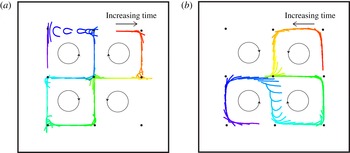
Flow-induced buckling of fibres is an important determinant of fibre transport. While fibre buckling in elementary shear and stagnation point flows is now relatively well understood (Becker & Shelley Reference Becker and Shelley2001; Young & Shelley Reference Young and Shelley2007; Kantsler & Goldstein Reference Kantsler and Goldstein2012; Wexler et al. Reference Wexler, Trinh, Berthet, Quennouz, du Roure, Huppert, Linder and Stone2013; see Lindner & Shelley (Reference Lindner, Shelley, Duprat and Stone2014) for a recent review), its influence in inhomogeneous flows is much less so. The achievement of such an understanding will be important, for example, to the eventual development of first-principles theories of flexible fibre suspensions. As a first step in this direction, Young & Shelley (Reference Young and Shelley2007) simulated the buckling-mediated transport of a flexible fibre through a given background 2D cellular flow. This background flow comprised sets of four counter-rotating vortices that periodically tiled the plane. They found that either fibres became trapped within the vortices of the cellular array or moved along the backbone of stable and unstable manifolds that connected the corresponding array of hyperbolic stagnation points; see figure 1. In the latter case, fibre transport behaved as a random walk with buckling of the fibre near the hyperbolic stagnation point acting as a coin flip for determining along which branch of the unstable manifold the fibre would depart. As a wandering fibre typically approaches the stagnation point along its compressive direction, Young and Shelley explained the observed buckling theoretically as arising from the instability of a nearly straight fibre under the viscously induced compressive axial load of the locally linear hyperbolic flow. This instability occurs beyond a critical strain rate of the linear flow, and is associated with a U-shaped deformation mode. Successive bifurcations at higher strain rates yield modes of higher spatial complexity.
Examples of typical transport and buckling dynamics of a fibre in a cellular array of counter-rotating vortices and associated hyperbolic stagnation points: simulations are shown in (a) (
 ${\it\eta}=2350$
) and experiments in (b) (
 ${\it\eta}=2230$
). Here
 ${\it\eta}$
is the adimensional strength of flow forcing. Time increases from red to blue in fibre colour. The circled arrows show the counter-rotating vortices that generate the stagnation points (indicated by black dots). The differences in the fibre shapes can be attributed to slight differences, particular to the experimental or simulational run, in the approach of the fibres to the stagnation point, as is explained in the text.

In an experimental instantiation of this theoretical model, Wandersman et al. (Reference Wandersman, Quennouz, Fermigier, Lindner and du Roure2010) created a viscous cellular flow consisting of a planar array of electromagnetically driven counter-rotating vortices, across which moved centimetric fibres made of a soft elastomer. They also observed fibre trapping in vortices and, when the fluid strain-rate was sufficiently high, transport and buckling of fibres through hyperbolic stagnation points. Kantsler & Goldstein (Reference Kantsler and Goldstein2012) investigated the deformation of a micrometric actin fibre held at a stagnation point created in a microfluidic cross-slot device where, unlike the experiments of Wandersman et al. (Reference Wandersman, Quennouz, Fermigier, Lindner and du Roure2010), transport dynamics does not play a role. They related the observed shapes to the predicted shape modes of the linear analysis of Young & Shelley, and showed that, given their small size, thermal fluctuations are contributory to the dynamics and have the role of smoothing out the transition to buckling. The role of thermal fluctuations in transport across cellular flow was further studied through simulations by Manikantan & Saintillan (Reference Manikantan and Saintillan2013), who showed that thermal fluctuations tended to increase trapping of fibres into vortices, and thus decreased transport.
The observations by Wandersman et al. (Reference Wandersman, Quennouz, Fermigier, Lindner and du Roure2010) identified a threshold to buckling that showed reasonable agreement with the predictions of linear analysis in a purely hyperbolic flow. However, these same observations also suggested that whether and how a fibre buckled was more complex than linear theory alone could account for. In this paper, we carry out a more detailed comparison of the computational model of Young & Shelley (Reference Young and Shelley2007) and the experimental set-up of Wandersman et al. (Reference Wandersman, Quennouz, Fermigier, Lindner and du Roure2010). We explore larger ranges in all experimentally controllable parameters, which extends the range of the fundamental control parameter, the elasto-viscous number
 ${\it\eta}$
, by an order of magnitude above that reached in Wandersman et al. (Reference Wandersman, Quennouz, Fermigier, Lindner and du Roure2010) of
 ${\it\eta}=900$
. We focus closely on the statistical relation between the state of the fibre entering a compression region (position, orientation, shape) and the development of a buckled state near the stagnation point. We show that when the simulations are performed to more closely follow the experimental protocols, the two systems show excellent quantitative concordance in their statistical behaviours, and that the theoretical model provides a very good basis from which to interpret the experimental observations. We show too that the system evinces a history dependence between buckling events that cannot be accounted for by a simple linear theory and that has not been noted in previous studies. In § 2 we introduce the theoretical model, the experimental set-up and the elements of the data analysis. In §§ 3 and 4 we discuss and compare the experimental and simulational observations.
2. Materials and methods
2.1. The theoretical model and its numerical simulation
Consider a slender fibre of radius
 $r$
and length
 $L$
that moves freely in a background velocity field
 $\boldsymbol{v}(\boldsymbol{x},t)$
. The fibre is assumed to be inextensible and elastic with flexural rigidity
 $B$
, and the fluid is described by the incompressible Stokes equations with viscosity
 ${\it\mu}$
. We represent the fibre by its centreline position
 $\boldsymbol{X}(s,t)$
, with
 $s$
the centreline arclength. For a slender fibre (i.e.
 ${\it\epsilon}=r/L\ll 1$
) we use local slender-body theory (Keller & Rubinow Reference Keller and Rubinow1976; Johnson Reference Johnson1980; Becker & Shelley Reference Becker and Shelley2001; Tornberg & Shelley Reference Tornberg and Shelley2004; Young & Shelley Reference Young and Shelley2007) to approximate its dynamics by the equations
 $$\begin{eqnarray}\displaystyle & \tilde{{\it\mu}}\left[\boldsymbol{X}_{t}-\boldsymbol{v}(\boldsymbol{X},t)\right]=\left(\boldsymbol{I}+\boldsymbol{X}_{s}\boldsymbol{X}_{s}^{T}\right)\left(\left(T\boldsymbol{X}_{s}\right)_{s}-B\boldsymbol{X}_{ssss}\right), & \displaystyle\end{eqnarray}$$
 $$\begin{eqnarray}\displaystyle & \boldsymbol{X}_{s}\boldsymbol{\cdot }\boldsymbol{X}_{ts}=0. & \displaystyle\end{eqnarray}$$
Here,
 $\tilde{{\it\mu}}=8{\rm\pi}{\it\mu}/(-\!\ln ({\it\epsilon}^{2}e))>0$
and subscripts refer to partial differentiation. Hence
 $\boldsymbol{X}_{s}$
is also the tangent to the fibre centreline. Equation (2.2) expresses that the arclength
 $s\in [0,L]$
is a material parameter, which is a consequence of inextensibility, and the tension
 $T$
is the quantity whose determination enforces that condition. In addition to tensile forces, we have bending forces which give rise to the high-order term
 $-B\boldsymbol{X}_{ssss}$
. We assume that the fibre is ‘free’, and so have the boundary conditions
 $\boldsymbol{X}_{ss}|_{s=0,L}=\boldsymbol{X}_{sss}|_{s=0,L}=\mathbf{0}$
and
 $T|_{s=0,L}=0$
. These guarantee that the fibre exerts zero net force and torque upon the surrounding fluid.
Scaling. We assume that the background velocity field has a characteristic length scale
 $W$
and strain rate
 $\dot{{\it\gamma}}$
, so that
 $\boldsymbol{v}(\boldsymbol{x},t)=W\dot{{\it\gamma}}\boldsymbol{u}(\boldsymbol{x}/W)$
. We now scale space on
 $L$
and time on
 $\dot{{\it\gamma}}^{-1}$
, and set
 ${\it\eta}\rightarrow \tilde{{\it\mu}}\dot{{\it\gamma}}L^{4}/B$
and
 ${\it\alpha}=L/W$
. Equation (2.1) becomes
 $$\begin{eqnarray}{\it\eta}\left[\boldsymbol{X}_{t}-{\it\alpha}^{-1}\boldsymbol{u}\left({\it\alpha}\boldsymbol{X}\right)\right]=\left(\boldsymbol{I}+\boldsymbol{X}_{s}\boldsymbol{X}_{s}^{T}\right)\left(\left(T\boldsymbol{X}_{s}\right)_{s}-\boldsymbol{X}_{ssss}\right),\end{eqnarray}$$
while (2.2) and the boundary conditions remain unchanged due to their homogeneity. Hence, the system has only two control parameters, one being the elasto-viscous number
 ${\it\eta}$
, which measures the flow strength relative to viscously modulated elastic relaxation. Like a Weissenberg number it can be written as the ratio of a fibre relaxation time
 ${\it\tau}_{R}=\tilde{{\it\mu}}L^{4}/B$
to a flow time scale
 ${\it\tau}_{F}=\dot{{\it\gamma}}^{-1}$
. The other control parameter is the normalized system length scale
 ${\it\alpha}^{-1}$
.
By applying the constraint (2.2) to (2.3), and through use of some simple differential geometric identities, we can replace (2.2) with an elliptic equation for the tension
 $T$
,
 $$\begin{eqnarray}2T_{ss}-\boldsymbol{X}_{ss}^{T}\boldsymbol{X}_{ss}T=-{\it\eta}\boldsymbol{X}_{s}^{T}\boldsymbol{{\rm\nabla}}\boldsymbol{v}\left(\boldsymbol{X}\right)\boldsymbol{X}_{s}-6\boldsymbol{X}_{sss}^{T}\boldsymbol{X}_{sss}-7\boldsymbol{X}_{ss}^{T}\boldsymbol{X}_{ssss}\end{eqnarray}$$
(see Tornberg & Shelley Reference Tornberg and Shelley2004), for which the boundary conditions
 $T_{s=0,L}=0$
are applied.
Linear behaviour near a stagnation point. For any linear background flow, a straight fibre with a parabolic tension distribution is an exact solution of (2.3) and (2.4). Of particular interest here is the stability of a straight fibre moving in the plane in the 2D linear hyperbolic flow
 $\boldsymbol{u}=(x,-y)$
. An illustrative and simple case is where the fibre is moving along the
 $y$
-axis, which is the direction of flow compression (Young & Shelley Reference Young and Shelley2007). In this case the linearized dynamics of transverse perturbations of the straight rod is variable coefficient but autonomous (see Lindner & Shelley Reference Lindner, Shelley, Duprat and Stone2014), and exponentially growing solutions satisfy the eigenvalue/vector relation
 $$\begin{eqnarray}{\it\lambda}f=f+sf_{s}+{\textstyle \frac{1}{4}}\left(s^{2}-{\textstyle \frac{1}{4}}\right)f_{ss}-{\it\eta}^{-1}f_{ssss},\end{eqnarray}$$
with
 $f_{ss}=f_{sss}=0$
at
 $s=0,1$
. While the variable coefficient nature prevents a closed-form solution, one can easily solve this eigenvalue/eigenfunction problem numerically (Young & Shelley Reference Young and Shelley2007; Lindner & Shelley Reference Lindner, Shelley, Duprat and Stone2014). With an eigenvalue solver we can track the system’s eigenvalues and eigenfunctions as
 ${\it\eta}$
, the effective viscosity or strain rate, is increased. For small
 ${\it\eta}$
the straight fibre is stable to perturbations. With increase in
 ${\it\eta}$
we find the successive crossing to the right half-plane of eigenvalues coupled to eigenfunctions associated with increasingly higher-order bending modes. The first three crossings occur at
 ${\it\eta}_{1}=153.2$
,
 ${\it\eta}_{2}=774.3$
and
 ${\it\eta}_{3}=1930$
, and the associated eigenmodes correspond respectively to the classical U-, S- and W-shaped buckling modes.
Numerical simulation. The two main difficulties that arise in numerically solving (2.3) and (2.4) are the temporal stiffness induced by the high number of spatial derivatives and accurately maintaining curve inextensibility in the discrete setting. In this study we will be considering 2D dynamics of the fibre in a 2D flow. In this setting both difficulties are easily handled by reformulating the dynamics in terms of the 2D curve’s tangent angle
 ${\it\nu}(s,t)$
, which satisfies
 $\boldsymbol{X}_{s}=\boldsymbol{e}({\it\nu})=(\cos {\it\nu},\sin {\it\nu})$
, where
 ${\it\nu}_{s}={\it\kappa}$
is the planar curvature. In terms of the tangent angle, (2.3) and (2.4) have the form
 $$\begin{eqnarray}\displaystyle & {\it\nu}_{t}=-{\it\eta}^{-1}{\it\nu}_{ssss}+g(s,t), & \displaystyle\end{eqnarray}$$
 $$\begin{eqnarray}\displaystyle & 2T_{ss}-{\it\nu}_{s}^{2}T=R(s,t), & \displaystyle\end{eqnarray}$$
 ${\it\nu}_{s}|_{s=0,1}={\it\nu}_{ss}|_{s=0,1}=T|_{s=0,1}=0$
. Here,
 $$\begin{eqnarray}\displaystyle & g=\boldsymbol{e}^{\bot }\left({\it\nu}\right)\boldsymbol{\cdot }\boldsymbol{v}_{s}+{\it\eta}^{-1}\left(9{\it\nu}_{s}^{2}{\it\nu}_{ss}+T{\it\nu}_{ss}+3{\it\nu}_{s}T_{s}\right), & \displaystyle\end{eqnarray}$$
 $$\begin{eqnarray}\displaystyle & R=-{\it\eta}\boldsymbol{e}\left({\it\nu}\right)\boldsymbol{\cdot }\boldsymbol{v}_{s}-\left(6{\it\nu}_{ss}^{2}+7{\it\nu}_{s}{\it\nu}_{sss}-{\it\nu}_{s}^{4}\right), & \displaystyle\end{eqnarray}$$
 $\boldsymbol{e}({\it\nu})=(\cos {\it\nu},\sin {\it\nu})$
and
 $\boldsymbol{e}^{\bot }({\it\nu})=(-\!\sin {\it\nu},\cos {\it\nu})$
, and where
 $\boldsymbol{v}_{s}$
is the arclength derivative of the background velocity
 $\boldsymbol{v}$
along the fibre. In this formulation the bending response appears through the high-order but linear term
 ${\it\nu}_{ssss}$
, while the function
 $g$
contains nonlinear, but lower-order, terms. While the curve geometry and its orientation are specified by
 ${\it\nu}$
, its absolute position is not, and so the centre-of-mass of the curve is evolved independently.
If (2.6) were integrated forward using an explicit time-stepping method then the bending term would induce the crippling stability constraint
 ${\rm\Delta}t<C{\rm\Delta}s^{4}$
, where
 ${\rm\Delta}t$
is the time step and
 ${\rm\Delta}s$
is the discretization length in
 $s$
. Hence, we use a second-order three-level (implicit) backward differentiation scheme to stably and accurately evolve
 ${\it\nu}$
,
 $$\begin{eqnarray}\displaystyle & \displaystyle \frac{1}{2{\rm\Delta}t}\left(3{\it\nu}^{m+1}-4{\it\nu}^{m}+{\it\nu}^{m-1}\right)=-{\it\eta}^{-1}{\it\nu}_{ssss}^{m+1}+\left(2g^{m}-g^{m-1}\right), & \displaystyle\end{eqnarray}$$
 $$\begin{eqnarray}\displaystyle & 2T_{ss}^{m}-\left({\it\theta}_{s}^{m}\right)^{2}T^{m}=R^{m}, & \displaystyle\end{eqnarray}$$
 ${\rm\Delta}t$
is the time step and
 $m$
refers to the time level
 $t_{m}=m{\rm\Delta}t$
. Because the bending term is treated implicitly, (2.10) constitutes a fourth-order boundary value problem for
 ${\it\nu}^{m+1}$
. We discretize these equations uniformly in
 $s$
using second-order accurate finite-difference formulae for all spatial derivatives. This includes the boundary conditions on
 ${\it\nu}$
which use compact one-sided formulae and which are applied at the
 $(m+1)^{st}$
time level (see Tornberg & Shelley Reference Tornberg and Shelley2004). This leads to a matrix equation for
 $T^{m}$
on the spatial mesh, which is solved first, followed by solution of a matrix equation for
 ${\it\nu}^{m+1}$
on the spatial mesh. This is accomplished efficiently by a sparse-matrix solver whose computational complexity scales linearly with the number of mesh points.
Periodic cellular flow. In this study we follow Young & Shelley (Reference Young and Shelley2007) and consider the doubly periodic incompressible cellular flow
 $$\begin{eqnarray}\boldsymbol{u}(\boldsymbol{x})=(\sin x\cos y,-\!\cos x\sin y).\end{eqnarray}$$
This cellular background flow comprises a periodic tiling of the 2D plane by a
 $2\times 2$
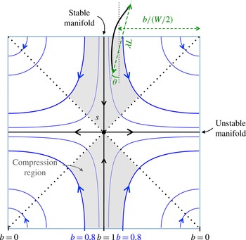
array of counter-rotating vortices centred upon a hyperbolic stagnation point whose stable and unstable manifolds separate the closed streamline vortices. The flow structure is shown schematically in figure 1.
A schematic defining quantities associated with entry into a compression zone. The distance
 $b$
to the centre of the closest vortex is normalized by
 $W$
. The deformation
 ${\it\lambda}$
is the ratio of the end-to-end distance and the fibre length
 $L$
. Here,
 ${\it\theta}$
is the angle between the end-to-end line and the stable manifold. The zone considered in the experiments and the simulations is limited by the four streamlines (two from the bottom and two from the top) corresponding to
 $b=0.8$
.

2.2. Experimental set-up
In our experiments an array of
 $4\times 5$
counter-rotating vortices, each of size
 $W=3~\text{cm}$
, is created using electromagnetic forcing of a viscous electrolyte (of depth 5 mm), as is described in detail in Wandersman et al. (Reference Wandersman, Quennouz, Fermigier, Lindner and du Roure2010). All our experiments are performed in a selected region, a
 $3\times 3$
lattice of stagnation points, where boundary effects are negligible. The electrolyte used is a 2:1 mixture of polyethylene glycol 1000 (Fluka) and purified water, into which NaCl is added up to saturation (viscosity
 ${\it\mu}=82\pm 5~\text{mPa}~\text{s}$
at
 $T=23\,^{\circ }\text{C}$
, surface tension
 ${\it\sigma}=43\pm 1~\text{mN}~\text{m}^{-1}$
and density
 ${\it\rho}_{e}=1.25\times 10^{3}~\text{kg}~\text{m}^{-3}$
). The applied electric current
 $I$
is tens of milliamperes.
The velocity field is measured by particle imaging velocimetry (using DAVIS software) and the flow created in this way is very well described by an equation of the form of (2.12), again as detailed by Wandersman et al. (Reference Wandersman, Quennouz, Fermigier, Lindner and du Roure2010). The experimental flow is found to be very nearly 2D, with the divergence of the 2D surface velocity being less than 5 % of the out-of-plane vorticity for all experiments. As detailed in figure 2, the flow around a hyperbolic streamline is compressive along streamlines near its incoming stable manifold (i.e. the shaded region), and extensional along streamlines near its outgoing unstable manifold. For this inhomogeneous flow, the compression/extension rate is maximal at the stagnation point itself, and zero at the vortex centres. The maximal compression/extension rate in the experiments is
 $\dot{{\it\gamma}}={\rm\pi}U_{0}(I)/W$
, where
 $U_{0}$
(in
 $\text{m}~\text{s}^{-1}$
) is a measured flow strength found to be linearly proportional to the applied electric current
 $I$
. In the range of velocities used, the Reynolds number (based on the fibre length) lies in the range
 $[0.1,0.95]$
. Inertial effects do not seem to play a major role in our findings.
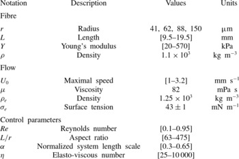
Experiments are performed with macroscopic fibres made from vinylpolysiloxane; their dimensions are given in table 1. The ratio of fibre length to cell size,
 ${\it\alpha}=L/W$
, varies from 0.3 to 0.65. The use of different samples allows us to vary the elastic bulk modulus of the fibre from
 $Y=20$
to 570 kPa. Determination of
 $Y$
using rheological measurements of the elastic shear modulus agreed well with independent beam bending experiments (Quennouz Reference Quennouz2013).
Experimental conditions.

We have shown before that the fibres produced in this way float on the surface of the electrolyte due to their lower density (Wandersman et al.
Reference Wandersman, Quennouz, Fermigier, Lindner and du Roure2010). More precisely, we have shown that the fibre is exactly half immersed and there is no meniscus. As a consequence, the motion and the deformation of the fibre are two-dimensional, being constrained at the surface of the liquid. As the interface is not deformed, the influence of surface tension on the dynamics of the fibre is negligible. The fact that the fibre is only half immersed reduces the viscous forces acting on it, and the elasto-viscous number will be corrected by a factor
 $1/2$
for comparison with simulations.
Pictures of the fibre are taken with a digital camera (PixeLINK,
 $1024\times 768$
) at 10 f.p.s. Using standard object detection procedures (ImageJ software) the shape of the fibre is captured from each frame. Data analysis is described in the next section.
2.3. Definitions
2.3.1. Data analysis
To study the dynamics along a fibre trajectory we define the passage of a fibre through the compression zone (the grey region in figure 2) as an elementary event. Both the experimental and the simulated data are treated identically. At each recorded time we have from the shape of the fibre its centre-of-mass position, its end-to-end distance and its angle
 ${\it\theta}$
between the end-to-end line and the stable manifold. The deformation
 ${\it\lambda}$
is the end-to-end distance normalized by the fibre length
 $L$
. Hence, if the fibre is nearly straight then
 ${\it\lambda}$
is near unity, while if it is highly bent then
 ${\it\lambda}$
is small. The fibre angle is taken as positive if the angle is in the direction of the streamlines and negative otherwise. As an example, in figure 2 the fibre has negative angle. From the temporal evolution of the centre-of-mass we can determine an entry event, when the fibre passes into a compression region. It is at this time that we record the entry distance of the fibre centre-of-mass to the centre of the neighbouring vortex and normalize it by
 $W/2$
. This normalized distance
 $b$
is unity on the stable manifold, and hence the distance of the fibre to the stable manifold is
 $1-b$
. We also record the entry angle
 ${\it\theta}$
and entry deformation
 ${\it\lambda}$
. As the fibre evolves freely, these parameters are set only at the beginning of a trajectory (through their initial values
 $b_{0}$
,
 ${\it\theta}_{0}$
and
 ${\it\lambda}_{0}$
). Along the trajectory, the position, orientation and deformation of the fibre are determined by its dynamics.
By following the deformation of the fibre during its passage in the compression region we can detect buckling: if the fibre deforms enough (
 ${\it\lambda}<0.8$
) then the event is counted as a buckling event. The criterion
 ${\it\lambda}<0.8$
was chosen such as to detect fibres that are deformed more strongly than a typical curvature of the streamlines (Wandersman et al.
Reference Wandersman, Quennouz, Fermigier, Lindner and du Roure2010). The number of buckling events is compared with the total number of events to calculate the buckling probability. Sometimes when the fibre has buckled in a previous event it is still substantially deformed. We do not consider such an event and so we disregard events for which the deformation at the entry satisfies
 ${\it\lambda}<0.88$
. This condition was chosen such as to ensure that fibres are sufficiently straight when entering the compression region. It should be noted that our results, presented in the following sections, are not very sensitive to the exact values used for the two criteria on
 ${\it\lambda}$
.
Because of the complex geometry of the flow we only consider an event if the fibre enters the compression region sufficiently close to the stable manifold (i.e.
 $b>0.8$
). This criterion allows us to consider the compression rate to be close to its maximal value along the stable manifold.
Conditions used for simulations. Two sets of simulations are performed. For the study of the buckling probability, we vary
 ${\it\eta}$
from 90 to 14 000. The ratio of the length of the fibres
 $L$
compared with the cell size
 $W$
is kept constant at
 ${\it\alpha}=L/W=0.4$
. Each value of
 ${\it\eta}$
is run for different initial conditions (
 $b_{0}=1$
, 0.95, 0.9, 0.85;
 ${\it\theta}_{0}=0^{\circ }$
, 3°, 6°) to obtain an ensemble of trajectories. To match the experiments, the length of the simulations is set so that the fibres pass through a compression region on average 60 times in one trajectory, a value comparable with what is achieved in the experiments.
The second set of simulations aims to study the impact of the parameters
 $b$
and
 ${\it\theta}$
on the buckling. For this we perform very short simulations, each containing only one event. The entry parameters are thus identical to the imposed initial conditions (
 $b_{0}$
,
 ${\it\theta}_{0}$
, with the fibre straight) and are varied over a large range:
 $0.8\leqslant b_{0}\leqslant 1$
and
 $-30^{\circ }\leqslant {\it\theta}_{0}\leqslant 30^{\circ }$
.
Conditions used for experiments. In a typical experiment the fibre is positioned initially as close as possible to the stable manifold. For the study of the buckling probability, the fibre then evolves freely until it leaves the useful region of the experiment. This corresponds to an average number of events comparable with the simulations, but with a strong variation between different experiments (typically between 1 and 200). We vary the length, radius and Young’s modulus of the fibres, as well as the maximal flow speed (see table 1).
To study the effect of the initial conditions, a specific set of experiments is performed with
 ${\it\eta}=2350$
and
 $L=12.5$
mm, corresponding to
 ${\it\alpha}=0.4$
. The initial conditions
 $b_{0}$
and
 ${\it\theta}_{0}$
are varied over a large range, comparable with the simulations.
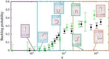
Buckling probability as a function of
 ${\it\eta}$
for both experiments (black squares) and simulations (green triangles). The error bars are the inverse of the square root of the number of corresponding trajectories. In the insets are typical shapes of fibres for various values of
 ${\it\eta}$
, including those at which the first, second and third buckling modes are observed (
 ${\it\eta}=175$
, 4075 and 8350 respectively). Theoretically predicted onset values for the first, second and third buckling modes (
 ${\it\eta}_{1}\approx 153.2$
,
 ${\it\eta}_{2}\approx 774.3$
and
 ${\it\eta}_{3}\approx 1930$
respectively) are shown as vertical lines. For both experiment and simulations, the buckling probability is only constructed for entry events where
 $b\geqslant 0.8$
. We estimate the error on the buckling probability from the number of events,
 $N$
, through
 $1/\sqrt{N}$
.

3. Buckling
3.1. Buckling probability
Figure 1 shows the transport and deformation of an elastic fibre in a viscous cellular flow, using one example from simulation (a) and another from experiment (b). For both, similar observations are made: the fibre is transported across the cellular network and along its path enters into successive compression regions. There, it interacts with the stagnation point flow, possibly deforming and buckling, and then exits. Our experiments show that the elasto-viscous number
 ${\it\eta}$
controls the buckling probability. This probability shows a slow increase from zero only after
 ${\it\eta}$
has exceeded a particular value. One might expect that since increasing
 ${\it\eta}$
corresponds to increasing the flow strength, buckling would become highly probable for large
 ${\it\eta}$
. However, for the ranges of
 ${\it\eta}$
studied in Wandersman et al. (Reference Wandersman, Quennouz, Fermigier, Lindner and du Roure2010) the buckling probability does not reach a saturated value at the highest values of
 ${\it\eta}$
used, much less approach unity.
In this study we significantly extend the range of the experimental parameters, in particular the fibre radius, length and bending modulus, and the flow viscosity and speed. This allows us to study the system at higher values of
 ${\it\eta}$
(see table 1). The buckling probability obtained from these new experiments is shown in figure 3 as a function of
 ${\it\eta}$
, averaged over all experimental conditions. A slow increase in the buckling probability is observed above a value of
 ${\it\eta}\approx 175$
. This is somewhat larger than the threshold value to linear instability,
 ${\it\eta}_{1}=153.2$
, in a linear hyperbolic flow (vertical line in figure 3). It should be noted that this slight discrepancy does not arise from the fact that the fibre does not spend enough time in the compression zone for the buckling to occur, as there is only one time scale
 $(W/U_{0})$
in our system corresponding to a typical residence time in the compression zone as well as to the inverse of the compression rate. The onset of positive probability is followed by an increase and saturation to an apparent limiting probability of approximately 0.4, well below unity. The shape of the experimental probability curve as a function of
 ${\it\eta}$
is quite robust for our experiments, and within the range of parameters used in these experiments little influence is seen of the fibre aspect ratio
 ${\it\epsilon}$
, the ratio
 ${\it\alpha}$
of fibre length to cell size or the Reynolds number.
Figure 3 also shows measurements of the buckling probability gleaned from an ensemble of numerical simulations, where both the initial fibre location and the orientation are varied. Their general agreement with experiment is surprisingly good. The simulations agree closely with the observed initial onset and rise of probability, though they yield a probability saturation level that is slightly higher than that in experiment. The simulations also show higher variability at high
 ${\it\eta}$
than the experiment. It is worth noting here that the experimental estimate of the onset value of
 ${\it\eta}$
could not be accounted for by linear theory without using the fact that viscous forces act only upon the immersed half of the floating fibre. Indeed, in our previous study (Wandersman et al.
Reference Wandersman, Quennouz, Fermigier, Lindner and du Roure2010) the onset value was calculated without this correction, yielding an onset value twice as large (350) as the present estimate.
3.2. The modes of deformation
Also displayed in figure 3 are experimentally observed sample shapes of fibres moving in compression regions. At small values of
 ${\it\eta}$
the fibres remain nearly straight. As
 ${\it\eta}$
is increased U-shaped buckling modes are first observed, as discussed above, at about
 ${\it\eta}=175$
, which is above the first linear threshold to instability at
 ${\it\eta}_{1}=153.2$
. As
 ${\it\eta}$
is increased, the U-shaped modes persist, but both the second and third modes, S- and W-shaped, also appear successively. They are first observed at approximately
 ${\it\eta}=4075$
and
 ${\it\eta}=8350$
respectively. These values are substantially larger than those predicted by the linear theory:
 ${\it\eta}_{2}\approx 774.3$
and
 ${\it\eta}_{2}\approx 1930$
(vertical lines in figure 3) respectively. A particularly large number of experiments were performed around the first onset to buckling. For the higher-order modes, fewer experimental observations were made close to their predicted threshold values of
 ${\it\eta}$
. This difference may explain why the higher-order modes were observed only for significantly larger values of
 ${\it\eta}$
(where their probability of appearance is presumably larger).
Kantsler & Goldstein (Reference Kantsler and Goldstein2012) also observe these buckling modes in their experiments on micron-scale actin fibres kept near the stagnation point of a cross-slot flow microfluidic device. As is observed here, the first transition to a U-shaped buckling mode is well captured by linear theory (despite the influence of thermal fluctuations). As is also observed here, the successive higher-order modes appear at successively higher values of flow forcing, although the precise onset of their appearance relative to the predictions of linear theory is unreported. The free transport of the fibre between compression regions in our set-up markedly increases the richness of the dynamics. As we show here, the appearance of buckling depends strongly on the entry conditions of the fibre into the compression region, and these entry conditions have a clear history dependence on the fibre’s previous encounters with compression.
4. Transport
We now investigate the influence of fibre transport through the system upon fibre buckling, and will show that the structure of the buckling probability curve reflects the complex dependences of buckling upon entry conditions and history.
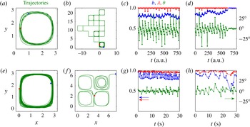
Two types of dynamics are typically observed at long times in both simulation and experiment. Examples are shown in figure 4(a,b,e,f). In one dynamical state, the fibre is trapped within a vortex (a,e) and roughly follows the closed streamline flow within. In the other dynamical state the fibre instead meanders across the lattice of vortices (b,f), transitioning from orbits about one vortex to orbits about another. Which of these two states is observed depends, in a non-trivial way, upon the fibre initial conditions
 $b_{0}$
and
 ${\it\theta}_{0}$
, and the control parameter
 ${\it\eta}$
. In the simulations, under certain conditions, a staircase-like motion of the fibre across the vortical array is also observed (not shown), although rarely. This dynamics is not observed in experiments, perhaps because of the small test section of the vortical array.
Examples of trajectories and corresponding time evolution of
 $b$
(blue),
 ${\it\lambda}$
(red) and
 ${\it\theta}$
(green): (a–d) show the simulation, (e–h) show the experiment. For the simulation: (a) shows a trapped fibre (
 ${\it\eta}=1200$
), (b) shows a meandering fibre (
 ${\it\eta}=350$
), (c) shows the evolution of entry values for the trapped fibre and (d) shows the evolution for the meandering fibre. For the experiment: (e) shows a trapped fibre (
 ${\it\eta}=3500$
), (f) shows a meandering fibre (
 ${\it\eta}=260$
), (g) shows the evolution of entry values for the trapped fibre and (h) shows the evolution for the meandering fibre. The red and blue dots in (a,b,e,f) mark the beginning (red) and end (blue) of the fibre orbits.

For the trapped fibres, as is suggested by our examples, both
 $b$
and
 ${\it\theta}$
can show oscillatory behaviours, essentially about a steady mean, that can span several passages through compression regions (figure 4
c,g). For those fibres with trajectories across the array, the parameters
 $b$
,
 ${\it\theta}$
and
 ${\it\lambda}$
(defined in figure 2) can also show oscillations, but also tend to evolve dynamically over long times (see figure 4
d,h). For example, the distance
 $1-b$
to the stable manifold often decreases over long time scales (i.e. note the increase of
 $b$
towards unity in the simulation example). Further, the angle
 ${\it\theta}$
often shows an oscillating behaviour between negative and positive values, with large jumps from negative to positive values, which defines the beginning of an oscillation. Our observation is that in many cases a buckling event is preceded by an entry event where
 ${\it\theta}$
is sufficiently negative, and hence inclined against the flow streamlines, to yield buckling. Buckling then produces a positive
 ${\it\theta}$
for the next entry, and it requires several passages before the entry angle becomes negative enough again for the fibre to buckle. While this is especially apparent for the simulations, the experiments (which are noisier) show the same basic feature.
We note that there is very little variation in
 ${\it\lambda}$
, and in most cases it can be neglected. We recall that we do not include events where the fibre is still strongly deformed upon entry.
5. Transport and buckling dynamics
Obviously the dynamics is very complicated, and an understanding of the origins of this complexity is beyond the scope of the present work. However, we find that a great deal can be learnt by quantifying the relation of buckling to temporal evolution of the entry values of
 $b$
and
 ${\it\theta}$
(and neglecting
 ${\it\lambda}$
as being comparatively unimportant).
To unambiguously study the influence of the entry values of
 $b$
and
 ${\it\theta}$
on buckling events during passage near a stagnation point, we performed a series of very short simulations with each consisting of only one entry event. We fixed the parameters at entry by setting the initial conditions
 $b_{0}$
and
 ${\it\theta}_{0}$
(with a straight fibre, i.e.
 ${\it\lambda}_{0}=1$
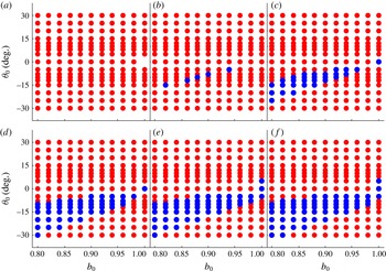
) and then determined whether buckling took place or not in the ensuing event. In this way we constructed the ‘phase diagrams’ (buckling versus non-buckling events) shown in figure 5, in the
 $b_{0}{-}{\it\theta}_{0}$
parameter space, for increasing values of
 ${\it\eta}$
. These maps are obtained from simulations, as it is far easier to explore the large range of parameters there.
Maps of buckling and not buckling in the
 $b_{0}{-}{\it\theta}_{0}$
parameter space for
 ${\it\eta}=145$
, 350, 700, 1400, 2000 and 3500 (a–f). Blue denotes buckling and red no buckling in the ensuing event.

With increasing
 ${\it\eta}$
the regions in the
 $b_{0}{-}{\it\theta}_{0}$
parameter space where buckling takes place (coloured in blue) change. No buckling is observed below the analytically predicted buckling threshold, and the region where buckling takes place increases in extent with increasing
 ${\it\eta}$
. In all cases, buckling only takes place for negative entry angles, except for fibres lying very close to the stable manifold, where the sign of
 ${\it\theta}$
is not very meaningful (as the sign is determined relative to the closest vortex, which is now somewhat ambiguous).
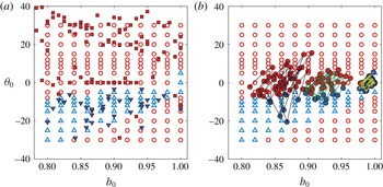
From a time-consuming set of experiments we also obtained a similar set of data for one value of
 ${\it\eta}$
above threshold (
 ${\it\eta}=2350$
) (figure 6
a). For these measurements the fibre was carefully positioned at varying distances from the stable manifold and varying initial angles, and released. We then recorded whether buckling took place during the ensuing event. Despite the many differences between the experimental set-up (use of finite-thickness fibres, an approximation of the background flow and a finite test section) and the simulations (use of local slender-body theory and an infinite system), we nonetheless found a good quantitative agreement between them. Thus, we will consider that the results obtained from the simulations are also valid in describing the experiments.
(a) Map of buckling as a function of
 $b_{0}$
and
 ${\it\theta}_{0}$
at the event entry for
 ${\it\eta}=2350$
. Experiments are represented by closed symbols (red squares, no buckling; blue down triangles, buckling) and simulations by open symbols (light red circles, no buckling; light blue up triangles, buckling). (b) Three simulated trajectories for different values of
 $b_{0}$
and
 ${\it\theta}_{0}$
, superposed upon the previous map. The lines reflect the time-dependent evolution of
 $b$
and
 ${\it\theta}$
. Each point has been coloured depending on buckling (blue) or no buckling (red) in the ensuing event.

We now investigate which parts of these maps are explored by fibres during transport, and whether the maps are predictive of buckling events. In figure 6(b) we have superimposed on the map temporal sequences of entry values
 $(b,{\it\theta})$
from trajectories of fibres released from three different initial conditions (
 $b_{0}$
,
 ${\it\theta}_{0}$
). Generally, a fibre spends time in regions of the phase diagram where buckling takes place, as well as in regions where no buckling takes place. Moreover, the phase diagram is a very good predictor as to whether the fibre actually buckles following the entry event.
That both buckling and no buckling regions are visited, even for values of
 ${\it\eta}$
well above the buckling threshold, is in agreement with our finding that the maximal observed buckling probability is significantly less than unity. That fibres buckle (or not) where the map predicts confirms that we are looking at the right variables. Only when the fibre is very close to the stable manifold (
 $b\sim 1$
) are some discrepancies observed (not visible from figure 6). Those rare buckling events that take place in regions where no buckling is predicted can be attributed to a deformation
 ${\it\lambda}$
that differs from unity. In this case, and only in this case, the deformation plays a role.
To obtain the buckling probability, we can disregard the temporal evolution, and simply count the number of buckling events compared with the total number of events. We found it useful to classify the different events in terms of the entry values
 $b$
and
 ${\it\theta}$
. In the following we choose to sort the different events simply based on the value of
 $b$
.
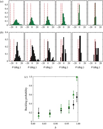
For
 ${\it\eta}=2350$
, figure 7 shows the histograms of angles
 ${\it\theta}$
over given ranges of
 $b$
for simulations (a) and experiments (b). The vertical red lines bound the region where buckling takes place according to the phase diagram in figure 5. One observes that the distribution of angles narrows as the fibre approaches the stable manifold (i.e.
 $b$
approaches 1). At the same time an increasingly large proportion of the entry angles lie within the region where buckling is observed. As a consequence, the buckling probability increases as
 $b$
approaches unity, as can be seen from figure 7(a,b), which shows the buckling probability from experiments and simulations as a function of
 $b$
for this special value of
 ${\it\eta}$
. It should be noted again that the exact value of the probability results from the combination of the parameter space map indicating where buckling takes place and the values of
 ${\it\theta}$
actually explored at a given
 $b$
. The buckling probability from the simulations reaches 1 for
 $b\sim 1$
. This is not observed in the experiments as a perfect alignment of the fibre with the stable manifold is probably not possible.
(a) Distribution of angles
 ${\it\theta}$
for different ranges of
 $b\;(0.80\leqslant b<0.85,0.85\leqslant b<0.90,0.90\leqslant b<0.95,0.95\leqslant b<0.97,0.97\leqslant b<0.99,0.99\leqslant b<1)$
from simulations (a) and experiments (b) for
 ${\it\eta}=2350$
. The red vertical lines indicate the regions where buckling takes place. (c) Corresponding buckling probability from simulations (green) and experiments (black) as a function of
 $b$
, chosen as the average value of each range of
 $b$
.

We now have all the elements needed to understand the shape of the probability curve presented in figure 3. First, the buckling probability increases with increasing
 ${\it\eta}$
due, in part, to the fact that the region in the
 $b{-}{\it\theta}$
parameter space where buckling can take place becomes larger with increasing
 ${\it\eta}$
. The exact shape of the probability curve as a function of
 ${\it\eta}$
is given by the distribution of
 $b$
and
 ${\it\theta}$
(and to a lesser extent
 ${\it\lambda}$
) during the trajectories of the fibres through the cellular flow. This link between the transport dynamics and the buckling of the fibre explains the smooth increase of the probability curve as well as the fact that the overall probability curve does not reach unity. It also shows the added complexity afforded by transport.
Underlying the apparent simplification gained by parametrizing the dynamics in terms of
 $b$
itself is that the dynamics of
 ${\it\theta}$
is fast (only a small number of events are needed to sample through the different values) while the dynamics of
 $b$
is slow. Hence, running experiments (or simulations) over different time scales can lead to different results in the overall buckling probability. Here, we achieved a good agreement between experiments and simulations because we matched both the initial conditions and the temporal lengths of the fibre trajectories.
6. Conclusion
In this paper we have studied the link between the transport and the buckling dynamics of an elastic fibre moving in a viscous cellular flow. We combined an experimental study using a centimetric fibre made from a soft elastomer in an electromagnetically driven viscous flow together with a computational study based on the dynamics of a slender Euler–Bernoulli elastic fibre moving in a Stokesian fluid. In both cases, the fibre is freely transported through an array of counter-rotating vortices and experiences a compressive load when approaching the hyperbolic stagnation points created by the vortex array. Buckling of the fibre leads to complex transport dynamics of the fibre through the array. A linear stability analysis describes the threshold of a buckling instability as a function of a non-dimensional viscosity (the elasto-viscous number
 ${\it\eta}$
). We showed that even above the buckling threshold, the fibre does not buckle with each passage near a stagnation point. We rationalized this observation by taking into account the fibre state when approaching the stagnation point. Buckling of a fibre depends not only upon the control parameter
 ${\it\eta}$
but also upon its entry distance and orientation to the unstable manifold. By simply taking into account these two parameters, fibre buckling can be quantitatively predicted.
These entry parameters are a consequence of the previous history of transport and buckling of the fibre through the array of stagnation points. In further studies it would be worthwhile to gain an understanding of the origins of the complex transport dynamics. The study of this simple model problem has revealed complex fibre dynamics that can only be explained by taking into account the coupling between deformation and transport. In the future this fundamental understanding should be useful to the understanding of even more complex flow situations.
Acknowledgements
The authors thank E. Wandersman and Y.-N. Young for fruitful discussions. M.J.S. acknowledges the support of the Department of Energy through grant DE-FG02-88ER25053.