1 Introduction
The degree to which turbulent zero pressure gradient (ZPG) boundary layer and pipe flows can be treated as similar has been a subject of debate for much of the last decade (e.g. see Jiménez & Hoyas Reference Jiménez and Hoyas2008; Monty et al.
Reference Monty, Hutchins, Ng, Marusic and Chong2009). While the no-slip condition forces similarity between boundary layers and pipes when scaled with friction velocity (
 $U_{\unicode[STIX]{x1D70F}}\equiv \sqrt{\unicode[STIX]{x1D70F}_{w}/\unicode[STIX]{x1D70C}}$
, where
 $\unicode[STIX]{x1D70F}_{w}$
is the shear stress at the wall and
 $\unicode[STIX]{x1D70C}$
is the fluid density) and length (
 $l_{v}\equiv \unicode[STIX]{x1D708}/U_{\unicode[STIX]{x1D70F}}$
, where
 $\unicode[STIX]{x1D708}$
is the kinematic viscosity of the fluid) sufficiently close to the wall, the wall distance at which this similarity breaks down (and which flow features begin to deviate) remains an open question. Possible sources of dissimilarity include differing outer boundary conditions (turbulent pipe centreline versus non-turbulent free stream in boundary layers), geometry (outer flow boundary exists along one-dimensional line in pipes versus two-dimensional plane in boundary layers) and differences in contributions to the mean momentum balance (mean pressure gradient in pipes versus mean advection in boundary layers).
Both physical experiments and numerical simulations have been conducted towards clarifying the onset and causes of discrepancies. Experimental results, however, are primarily limited to those pertaining to the streamwise component of velocity – largely owing to the relative difficulty of measuring the other two components. Monty et al. (Reference Monty, Hutchins, Ng, Marusic and Chong2009) compared streamwise velocity spectra and the first four statistical moments of the streamwise velocity collected in pipe, channel and boundary layer flows at a friction Reynolds number of approximately 3000, where
 $Re_{\unicode[STIX]{x1D70F}}\equiv U_{\unicode[STIX]{x1D70F}}\unicode[STIX]{x1D6FF}/\unicode[STIX]{x1D708}$
and
 $\unicode[STIX]{x1D6FF}$
refers to the boundary layer height and/or the pipe radius/channel half-height, where applicable. They found that the statistical structure of the streamwise velocity fluctuations was virtually the same in all three flows from the wall to at least
 $0.5\unicode[STIX]{x1D6FF}$
. Despite this statistical invariance, the authors also found that eddies with streamwise wavelength
 ${\gtrsim}10\unicode[STIX]{x1D6FF}$
contribute more to the streamwise variance in the log layer for internal (pipe/channel) flows than they do for external (boundary layer) flows. That the streamwise statistical invariance is apparently maintained despite the difference in spatial organization motivates an investigation into the behaviours of other flow variables such as the cross-stream velocities and the vorticity.
While experimentally determined profile statistics of the wall-normal and spanwise/azimuthal components of velocity are available independently for both pipes and boundary layers, no single experimental study has presented data for both flows acquired with the same probe and data-reduction scheme under matched probe resolution and Reynolds number conditions. Consequently, it is difficult to differentiate between flow-dependent features and experimental scatter based on a collection of existing experimental results alone. This is illustrated in Jiménez & Hoyas (Reference Jiménez and Hoyas2008), where a selection of existing experimental data from both internal and external flows are presented alongside the results of a set of direct numerical simulations (DNS) of channel flow. One way to approach the issue of experimental scatter is to compare DNS results of internal and external flows directly, as in Jiménez et al. (Reference Jiménez, Hoyas, Simens and Mizuno2010) and Chin, Monty & Ooi (Reference Chin, Monty and Ooi2014). Such comparisons, however, have thus far been limited to friction Reynolds numbers of
 $Re_{\unicode[STIX]{x1D70F}}\approx 1000$
or less. Since it is unclear whether wall flows of
 $Re_{\unicode[STIX]{x1D70F}}\lesssim 1000$
contain a well-developed inertial layer (Morrill-Winter, Philip & Klewicki Reference Morrill-Winter, Philip and Klewicki2017), it remains to be seen whether features observed in the transverse velocity variance profiles persist at higher
 $Re_{\unicode[STIX]{x1D70F}}$
. Furthermore, to the authors’ knowledge, third- and fourth-order statistics of the transverse velocity components have not yet been reported in a comparative study of internal and external flows. Such statistics contain valuable information about the probability distribution functions of turbulence quantities, as they clarify the relative dominance of positive versus negative, or large versus small fluctuations, and the dependence of these measures on wall distance. Additionally, the normalized third- and fourth-order moments and, in particular, how these compare to those associated with Gaussian processes, may be used to evaluate existing models of wall-bounded flow, and inform new models/modifications to existing models.
Differences in wake structure between internal and external flows have been discussed in the context of turbulent/non-turbulent intermittency since the early studies by Schubauer (Reference Schubauer1954) and Klebanoff (Reference Klebanoff1955). Both authors asserted that the distribution of velocity fluctuations was most likely the same in the ‘turbulent’ patches of the boundary layer as they are in the pipe. External boundary layers are bounded by irrotational potential flow, the entrainment of which is commensurate with flow development in the streamwise direction. Fully developed internal flows, however, have no such source of irrotational flow and do not develop in the streamwise direction. Despite this fact, Kwon et al. (Reference Kwon, Philip, de Silva, Hutchins and Monty2014) identified a large-scale region, or ‘quiescent core’, in channel flows at
 $Re_{\unicode[STIX]{x1D70F}}\approx 1000$
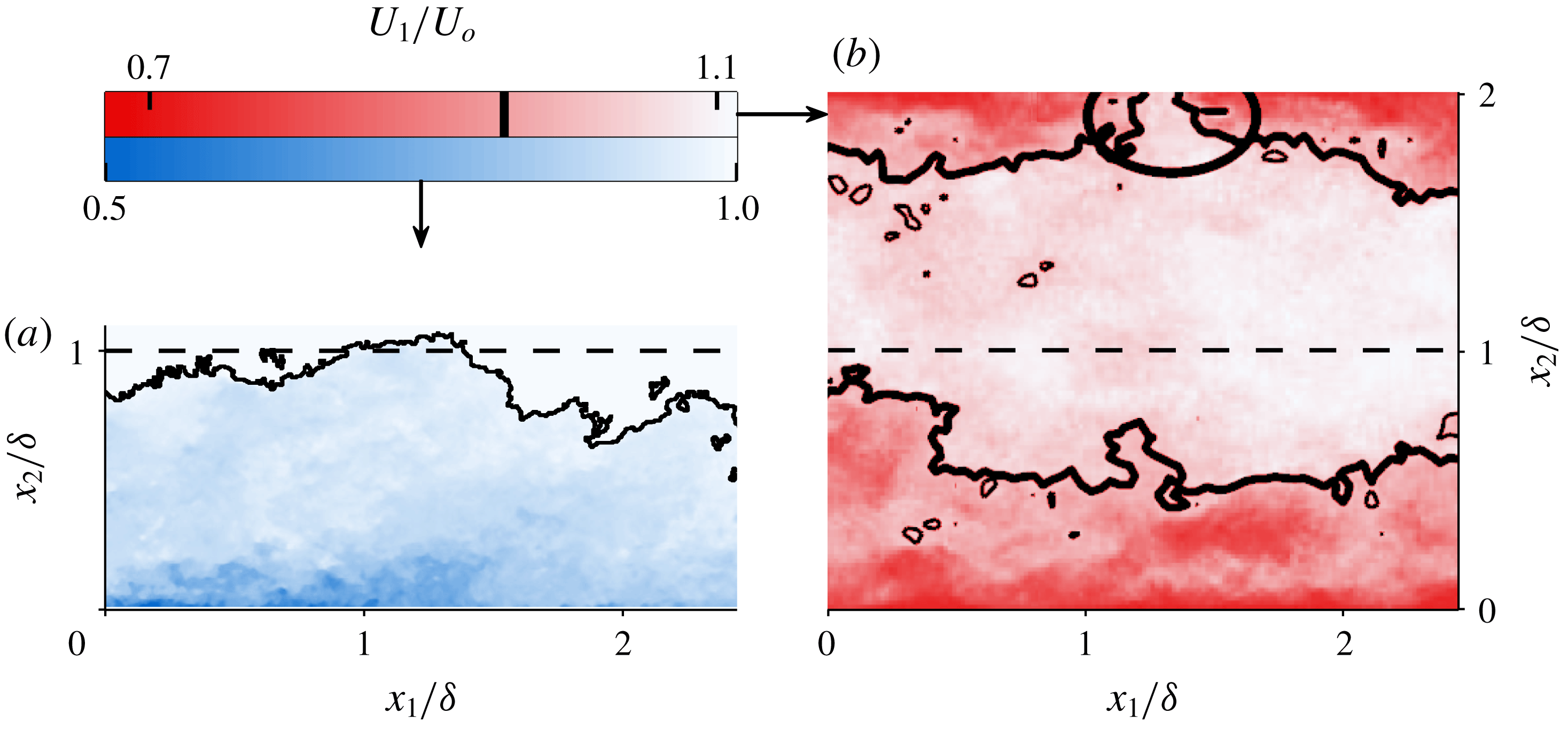
–4000 having characteristics reminiscent of those of the boundary layer free stream. Example snapshots of the turbulent/non-turbulent interface (TNTI) in a boundary layer from Chauhan et al. (Reference Chauhan, Philip, de Silva, Hutchins and Marusic2014b
) and the quiescent-core boundary in a channel from Kwon et al. (Reference Kwon, Philip, de Silva, Hutchins and Monty2014) are shown in figures 1(a) and 1(b), respectively. Although the boundary of the quiescent core is qualitatively similar to the TNTI, its influence (if any) on turbulence statistics at Reynolds numbers higher than
 $Re_{\unicode[STIX]{x1D70F}}\approx 4000$
is presently unknown. In this study, we show that normalized third- and fourth-order statistical moments of pipe flow are indicative of intermittency associated with a quiescent core, and that differences in the intermittency between pipe and boundary layer flow can explain many of the observed differences between the two flows.
In the present experiments, we simultaneously measure all components of velocity and vorticity in boundary layer and pipe flows for
 $5000\lesssim Re_{\unicode[STIX]{x1D70F}}\lesssim 10\,000$
. Thus, the present data set allows for differentiation between ‘turbulent’ and ‘non-turbulent’ patches by their instantaneous enstrophy rather than an analogue measure based, for example, on the streamwise velocity. As such, another aim of this study is to compare the prevalence and structure of quasi-‘non-turbulent’ flow in pipes and boundary layers as well as the vortical properties of the ‘turbulent’ patches.
(a) Snapshot adapted from Chauhan et al. (Reference Chauhan, Philip, de Silva, Hutchins and Marusic2014b
) showing turbulent/non-turbulent interface in a ZPG boundary layer at
 $Re_{\unicode[STIX]{x1D70F}}\approx 12\,300$
. Interface location in (a) based on threshold of local turbulence kinetic energy (see Chauhan et al.
Reference Chauhan, Philip, de Silva, Hutchins and Marusic2014b
). (b) Snapshot adapted from Kwon et al. (Reference Kwon, Philip, de Silva, Hutchins and Monty2014) showing boundaries of the quiescent core in channel flow at
 $Re_{\unicode[STIX]{x1D70F}}\approx 1000$
. Quiescent-core boundary based on
 $U_{1}/U_{o}=0.95$
contour, where
 $U_{1}$
is the mean streamwise velocity and
 $U_{o}$
is the centreline velocity for the channel, and the free-stream velocity for the boundary layer. Coordinates
 $x_{1}$
and
 $x_{2}$
refer to the streamwise and wall-normal directions, respectively. Ellipse in (b) highlights instance where the quiescent core boundary nearly reaches the wall.

Throughout the rest of this text, subscripts 1, 2 and 3 refer to the streamwise, wall-normal and spanwise/azimuthal directions, respectively. Superscript ‘
 $+$
’ indicates normalization by viscous scales. The position
 $x_{2}=0$
refers to the wall in both the pipe and boundary layer cases. Overbar
 $\overline{(\cdot )}$
or capitalization denotes a time-averaged quantity, superscript prime
 $(\cdot )^{\prime }$
or lower case denotes a fluctuating quantity, and a tilde
 $\tilde{(\cdot )}$
denotes a total quantity. The following are examples of the notation used throughout: the total streamwise velocity can be decomposed as
 $\tilde{u} _{1}=U_{1}+u_{1}$
; the mean Reynolds shear stress can be expressed as
 $\overline{u_{1}u_{2}}$
; and the fluctuating component of the instantaneous Reynolds shear stress can be expressed as
 $(u_{1}u_{2})^{\prime }$
.
2 Experiments
2.1 Facilities
The present data were collected as part of a collaborative effort between the authors at the Center for International Collaboration in Long Pipe Experiments (CICLoPE) and the Flow Physics Facility (FPF) – respectively the largest-scale turbulent pipe flow and zero pressure gradient boundary layer facilities in existence. The former is a closed-loop system that generates a fully developed turbulent pipe flow in a 90 cm diameter test section over a development length of 110.9 m (i.e. a length-to-diameter ratio of 123.2). The loop includes a heat exchanger which keeps the flow temperature constant to within
 $\pm 0.2\,^{\circ }\text{C}$
, even for measurement durations in excess of 9 h. A detailed design of CICLoPE can be found in Talamelli et al. (Reference Talamelli, Persiani, Fransson, Alfredsson, Johansson, Nagib, Rüedi, Sreenivasan and Monkewitz2009), and initial velocity measurements are reported in Örlü et al. (Reference Örlü, Fiorini, Segalini, Bellani, Talamelli and Alfredsson2017). The FPF, first characterized in Vincenti et al. (Reference Vincenti, Klewicki, Morrill-Winter, White and Wosnik2013), is an open circuit zero pressure gradient wind tunnel in which the boundary layer grows continuously over a streamwise development length of 72 m, ultimately achieving boundary layer heights of up to 75 cm. The spatial development of the boundary layer over this long fetch permits the outer flow scale to be set to any value up to the maximum by establishing a fixed measurement station at the corresponding streamwise location. The friction velocity at any streamwise location is constant to within within 0.5 % for the central 5 m of the total 6 m test section span, while the sloped ceiling maintains the free-stream velocity as constant to within
 $\pm 1\,\%$
over the range used herein (Vincenti et al.
Reference Vincenti, Klewicki, Morrill-Winter, White and Wosnik2013).
Both facilities are ideal for high-fidelity measurements of high Reynolds number flows, as their physical size allows for the generation of a wide range of energy-containing scales without the smallest of those being unresolvable via conventional measurement techniques. The two facilities are also particularly well suited for direct flow comparisons with one another, as the operational flow speeds and physical dimensions make it possible to simultaneously match both inner and outer flow scales at considerable Reynolds numbers.
It is worth noting that the open-circuit design of the FPF presents additional experimental challenges relative to smaller, indoor (or closed-loop) facilities. As the inflow is drawn from the atmosphere, compensation is needed for the calibration drift associated with changes in atmospheric temperature over the course of each measurement. The FPF data also show slight departures from canonical behaviour in the wake of the generated boundary layer (e.g. see Vincenti et al.
Reference Vincenti, Klewicki, Morrill-Winter, White and Wosnik2013). Although we do not believe that these factors impact the conclusions of this study, additional boundary layer measurements collected in the High Reynolds Number Boundary Layer Wind Tunnel (HRNBLWT) at the University of Melbourne (e.g. see Kulandaivelu Reference Kulandaivelu2012) are included in appendix A for comparison. The HRNBLWT is an indoor open-circuit ZPG boundary layer wind tunnel with a streamwise development length of 27 m, which allows for generation of a boundary layer up to 35 cm thick. As such, to achieve matched spatial resolution with the FPF and CICLoPE measurements, the HRNBLWT measurements are collected at Reynolds numbers approximately
 $2/3$
as large as those obtained at the FPF and the CICLoPE.
2.2 Measurement probe
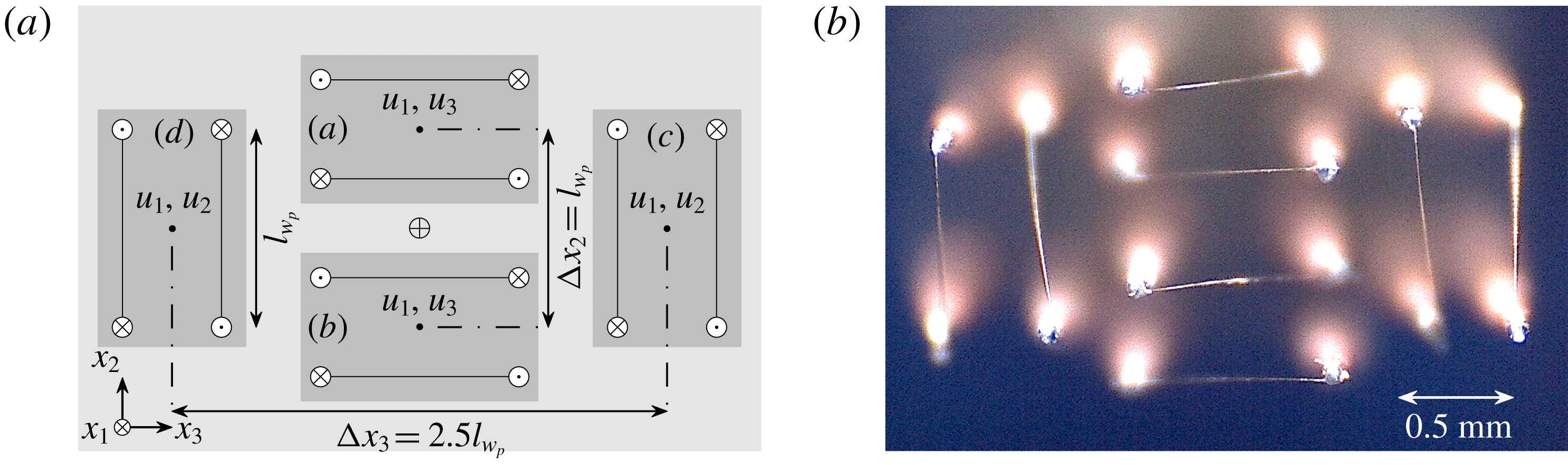
All of the data presented herein were acquired via a multi-element hot-wire anemometry probe consisting of 8 independent sensing elements. The design of this probe and its capacity to capture key aspects of the velocity and vorticity time series in turbulent boundary layers are discussed in detail in Zimmerman, Morrill-Winter & Klewicki (Reference Zimmerman, Morrill-Winter and Klewicki2017). The arrangement of the sensing elements, shown in figure 2, is similar to the arrangement deployed by Antonia, Zhou & Zhu (Reference Antonia, Zhou and Zhu1998) in a grid-generated turbulent flow. Several modifications were made to this design to reduce the overall measurement volume and better suit operation in wall-bounded flows. These include a reduction of the relative spacing between sub-arrays (a) and (b) to prioritize resolution of the
 $x_{2}$
gradients, and the use of gold-plated tungsten wire in place of platinum-core Wollaston wire.
(a) Probe schematic with relative dimensions. (b) Front-on picture of actual probe. Labels (a–d) in (a) refer to
 $\times$
-array ‘sub-arrays’ as referenced throughout text. Probe centroid is indicated by
 $\oplus$
. Reference length
 $l_{w_{p}}$
is the sensor length
 $l_{w}$
projected into the
 $x_{2}$
–
 $x_{3}$
plane, which for this study is fixed at 0.8 mm.

For illustrative purposes, it is useful to describe the present probe as being composed of four individual
 $\times$
-wire sub-arrays. The probe schematic shown in figure 2 is consistent with this description and demonstrates one way in which both the velocity and vorticity vectors may be obtained about the centroid of the measurement volume. In contrast to some other multi-element hot-wire probes deployed in wall-bounded flows (e.g. see the review of Wallace & Vukoslavčević (Reference Wallace and Vukoslavčević2010)), the individual sub-array centroids of the present probe are symmetric about the overall measurement volume centroid. The advantage of this symmetry is that all gradient estimates (and thus vorticity component estimates) can be obtained via central finite differences about a single common point. Another advantage of the present design is the focus on resolving the vorticity vector specifically rather than the entire velocity gradient tensor. Forgoing measurement of two normal gradients (
 $\unicode[STIX]{x2202}u_{2}/\unicode[STIX]{x2202}x_{2}$
and
 $\unicode[STIX]{x2202}u_{3}/\unicode[STIX]{x2202}x_{3}$
) eliminates the practical requirement for each sub-array to estimate all three components of velocity simultaneously, the merits of which are evidenced by the velocity component variances reported in Zimmerman et al. (Reference Zimmerman, Morrill-Winter and Klewicki2017).
2.3 Calibration
Data collected from a two-step in situ calibration procedure are combined to characterize the response of each sensor to a range of flow angles and speeds expected to be encountered in the profile scans. In the first procedure, the sensors are traversed to a position where they will encounter quasi-uniform flow (
 $x_{2}>\unicode[STIX]{x1D6FF}_{99}$
in the boundary layer and
 $x_{2}=0.93R$
in the pipe). Note that the mean streamwise velocity at
 $x_{2}=0.93R$
(the location corresponding to the maximum extent of the traversing apparatus) differs from the centreline velocity by less than 0.3 % according to the DNS dataset of Chin et al. (Reference Chin, Monty and Ooi2014). The sensors are then exposed to between 9 and 11 flow speeds ranging from approximately
 $1~\text{m}~\text{s}^{-1}$
at the low end to
 $1.25U_{o}$
at the high end, where
 $U_{o}$
is the velocity in either the free stream or at the pipe centreline. The flow speeds in both cases are measured by Pitot-static tubes. A third-order polynomial is then fitted to the median hot-wire voltage versus median flow speed data points. The median is used rather than the mean to remove the influence of non-uniformity in the calibrating flow, (e.g. non-zero turbulence intensity in the pipe centreline). This procedure is performed before and after every profile scan, providing two reference points for temperature-based interpolation of a single response curve for each profile measurement
 $x_{2}$
position. A key advantage of this procedure is that the flow incidence is known to be
 $0^{\circ }$
relative to the position of the probe during the actual profile scan.
The second step of the calibration procedure utilizes an in-house built articulating jet first described in Morrill-Winter & Klewicki (Reference Morrill-Winter and Klewicki2013) to generate uniform flow at both yaw and pitch angles across the same range of flow speeds as the quasi-uniform tunnel calibrations described above. Data are collected at thirteen pitch and thirteen yaw angles at each speed. Tangential cooling coefficients
 $k$
(Jorgensen Reference Jorgensen1971), and effective cooling angles
 $\unicode[STIX]{x1D6FC}$
(Bradshaw Reference Bradshaw1971), are determined for each sensor at each speed and used in the following expression to describe the sensor response:
 $$\begin{eqnarray}\displaystyle u_{e}^{2}=\underbrace{(u_{1}\sin \unicode[STIX]{x1D6FC}-u_{i}\cos \unicode[STIX]{x1D6FC})}_{u_{N}}^{2}+k^{2}\underbrace{(u_{1}\cos \unicode[STIX]{x1D6FC}+u_{i}\sin \unicode[STIX]{x1D6FC})}_{u_{T}}^{2}, & & \displaystyle\end{eqnarray}$$
where
 $u_{e}$
is the ‘effective’ cooling velocity and
 $u_{i}$
is either
 $u_{2}$
or
 $u_{3}$
(depending on the orientation of the sensor), and the subscripts
 $N$
and
 $T$
refer to the directions normal and tangential to the sensor, respectively. The original expression suggested by Jorgensen (Reference Jorgensen1971) includes another term that describes the effect of ‘bi-normal’ cooling velocity, but this term is neglected here (Zimmerman et al.
Reference Zimmerman, Morrill-Winter and Klewicki2017). The use of (2.1) with speed-dependent cooling coefficients collapses the jet calibration data onto a single curve with errors typically less than 1 % for speeds above
 $2~\text{m}~\text{s}^{-1}$
. While the jet calibration is theoretically sufficient to describe the entire probe response, there are two practical difficulties associated with the jet calibration that necessitate the tunnel calibration (i.e. the first step). First, it was shown in Zimmerman et al. (Reference Zimmerman, Morrill-Winter and Klewicki2017) that even very minor misalignment of the jet relative to the mean flow could result in substantial errors in reported Reynolds shear stress components. Second, the fan which generates the calibrating jet flow can heat the air by several degrees Celsius, resulting in a shifted speed response curve. Both of these issues are circumvented by forcing the jet calibration surface to fall upon (at
 $0^{\circ }$
nominal flow incidence) the tunnel calibration curve.
2.4 Data reduction
Raw sensor output is reduced to velocity and shear gradients about the centroid of the measurement volume by solving two closed four-equation four-unknown systems. These systems, obtained from (2.1), and given in (2.2) and (2.3), are first-order Taylor series expansions of two-dimensional velocity in the direction normal to the velocity plane for each set of four coplanar sensing elements.
 $$\begin{eqnarray}\displaystyle u_{e_{j}}^{2} & = & \displaystyle \left[\left(u_{1}+h_{j}\frac{\unicode[STIX]{x2202}u_{1}}{\unicode[STIX]{x2202}x_{2}}\right)\sin (\unicode[STIX]{x1D6FC}_{j})-\left(u_{3}+h_{j}\frac{\unicode[STIX]{x2202}u_{3}}{\unicode[STIX]{x2202}x_{2}}\right)\cos (\unicode[STIX]{x1D6FC}_{j})\right]^{2}+\cdots \nonumber\\ \displaystyle & & \displaystyle k_{j}^{2}\left[\left(u_{1}+h_{j}\frac{\unicode[STIX]{x2202}u_{1}}{\unicode[STIX]{x2202}x_{2}}\right)\cos (\unicode[STIX]{x1D6FC}_{j})+\left(u_{3}+h_{j}\frac{\unicode[STIX]{x2202}u_{3}}{\unicode[STIX]{x2202}x_{2}}\right)\sin (\unicode[STIX]{x1D6FC}_{j})\right]^{2},\end{eqnarray}$$
 $$\begin{eqnarray}\displaystyle u_{e_{j}}^{2}=\left[\left(u_{1}+h_{j}\frac{\unicode[STIX]{x2202}u_{1}}{\unicode[STIX]{x2202}x_{3}}\right)\sin (\unicode[STIX]{x1D6FC}_{j})-\left(u_{2}+h_{j}\frac{\unicode[STIX]{x2202}u_{2}}{\unicode[STIX]{x2202}x_{3}}\right)\cos (\unicode[STIX]{x1D6FC}_{j})\right]^{2}+\cdots & & \displaystyle \nonumber\\ \displaystyle k_{j}^{2}\left[\left(u_{1}+h_{j}\frac{\unicode[STIX]{x2202}u_{1}}{\unicode[STIX]{x2202}x_{3}}\right)\cos (\unicode[STIX]{x1D6FC}_{j})+\left(u_{2}+h_{j}\frac{\unicode[STIX]{x2202}u_{2}}{\unicode[STIX]{x2202}x_{3}}\right)\sin (\unicode[STIX]{x1D6FC}_{j})\right]^{2}. & & \displaystyle\end{eqnarray}$$
Equation (2.2) is thus appropriate for the four wires oriented in sub-arrays
 $a$
and
 $b$
, and (2.3) is appropriate for those in
 $c$
and
 $d$
. Initial guesses are produced from
 $\times$
-array outputs of sub-arrays
 $a$
,
 $b$
,
 $c$
and
 $d$
from figure 2. These initial
 $\times$
-array outputs are obtained via lookup tables that are populated based on (2.1) and the third-order polynomial fit relating voltage to
 $u_{e}$
mentioned above. Note that the index
 $j$
in (2.2) and (2.3) indicates an individual sensing element (1–8), and
 $h_{j}$
indicates the separation between sensor ‘
 $j$
’ and the centroid in the direction of the Taylor series expansion. For example, if elements 1 and 2 are in sub-array
 $a$
, then
 $h_{1}=(3/4)l_{w_{p}}$
and
 $h_{2}=(1/4)l_{w_{p}}$
(see figure 2).
At each measurement time instant, we obtain
 $u_{e_{j}}$
for each wire based on its voltage output and
 $k_{j}$
, and
 $\unicode[STIX]{x1D6FC}_{j}$
based on the initial
 $\times$
-array solution. These values are substituted into (2.2) and (2.3) along with the initial
 $\times$
-array solutions for the velocities and their gradients, and the systems are solved via an iterative nonlinear least-squares algorithm. The output of this solution method is the three velocity components and the four cross-stream shear gradients
 $\unicode[STIX]{x2202}u_{1}/\unicode[STIX]{x2202}x_{2}$
,
 $\unicode[STIX]{x2202}u_{3}/\unicode[STIX]{x2202}x_{2}$
,
 $\unicode[STIX]{x2202}u_{1}/\unicode[STIX]{x2202}x_{3}$
, and
 $\unicode[STIX]{x2202}u_{2}/\unicode[STIX]{x2202}x_{3}$
. The advantage of the systems given by (2.2) and (2.3) compared to a typical
 $\times$
-array method is that the assumption of uniform flow across
 $\times$
-wire pairs is relaxed to one that allows a linear velocity gradient across the measurement volume. This reduces the aliasing associated with non-uniform flow across the
 $\times$
-wire domain (Zimmerman et al.
Reference Zimmerman, Morrill-Winter and Klewicki2017). The remaining shear gradients not given by (2.2) or (2.3) (i.e. those taken in the streamwise direction) are estimated via Taylor’s frozen turbulence hypothesis, using the local mean velocity as the convection velocity. These six shear gradients are then used to compute all three instantaneous vorticity components.
All statistics presented herein are computed from velocity time series obtained via (2.2) and (2.3) with the exception of the statistical moment profiles of
 $u_{2}$
and
 $u_{1}u_{2}$
, which are obtained via the same lookup-table approach as is used to produce initial guesses for (2.2) and (2.3). Although solving (2.3) produces a higher-fidelity estimate of
 $u_{2}$
about the probe centroid than any linear combination of outputs from sub-arrays
 $c$
and
 $d$
, there is no particular benefit associated with computing
 $u_{2}$
statistics from a centralized measurement. The probe-centred signal is, however, preferable for the calculation of the
 $\unicode[STIX]{x2202}u_{2}/\unicode[STIX]{x2202}x_{1}$
component of
 $\unicode[STIX]{x1D714}_{3}$
(for example), since the collocation of the
 $\unicode[STIX]{x2202}u_{2}/\unicode[STIX]{x2202}x_{1}$
and
 $\unicode[STIX]{x2202}u_{1}/\unicode[STIX]{x2202}x_{2}$
gradient estimates significantly improves the fidelity of the overall
 $\unicode[STIX]{x1D714}_{3}$
estimate (Zimmerman et al.
Reference Zimmerman, Morrill-Winter and Klewicki2017).
2.5 Measurement parameters
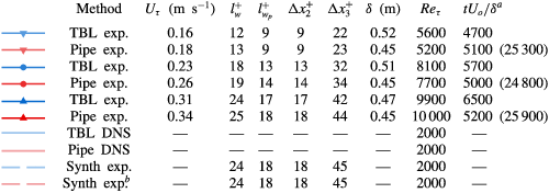
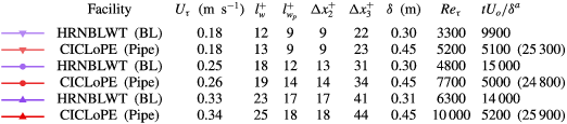
The relevant measurement parameters of this study are summarized in table 1. The friction velocity
 $U_{\unicode[STIX]{x1D70F}}$
in the boundary layer case is determined by the composite fit of Chauhan, Monkewitz & Nagib (Reference Chauhan, Monkewitz and Nagib2009) with the von Kármán and intercept constants chosen as
 $\unicode[STIX]{x1D705}=0.39$
and
 $B=4.3$
, respectively (Marusic et al.
Reference Marusic, Monty, Hultmark and Smits2013). An analogue of the standard
 $\unicode[STIX]{x1D6FF}_{99}$
is used due to the slight non-zero curvature of the mean velocity profile in the FPF boundary layer free stream (cf. figure 3 in the next section). Since the inner-normalized streamwise velocity variance profile as a function of
 $x_{2}/\unicode[STIX]{x1D6FF}$
follows a single
 $Re$
-independent curve in the vicinity of
 $\unicode[STIX]{x1D6FF}_{99}$
, at least over the
 $Re$
-range considered herein (e.g. see Marusic et al.
Reference Marusic, Chauhan, Kulandaivelu and Hutchins2015),
 $\unicode[STIX]{x1D6FF}_{99}$
is identified in the present ZPG cases as the position where the inner-normalized streamwise variance equals 0.257 – its value at the position corresponding to
 $U=0.99U_{o}$
based on the DNS results of Sillero, Jiménez & Moser (Reference Sillero, Jiménez and Moser2013). Throughout the rest of this text,
 $\unicode[STIX]{x1D6FF}_{99}$
will refer to this analogue definition. The friction velocity in the pipe is obtained from direct measurements of the pressure drop using 18 ports located along the entire working section. Wall position in both measurements is first determined with a microscope to within
 $\pm 0.1$
mm and subsequently tracked via an optical encoder on the traversing apparatus. Integration of the measured mean velocity profiles yields the average, or bulk velocity, from which (along with the measured mean pressure gradient) the friction factor
 $\unicode[STIX]{x1D706}$
and Reynolds number
 $Re_{D}$
based on pipe diameter and bulk velocity are obtained. The present measured values of
 $\unicode[STIX]{x1D706}$
(for each measured
 $Re_{D}$
) are all within 0.75 % of those based on the curve suggested by McKeon et al. (Reference McKeon, Swanson, Zagarola, Donnelly and Smits2004) at the corresponding values of
 $Re_{D}$
.
Also summarized in table 1 are the numerical data sets used for comparison. These include the boundary layer DNS of Sillero et al. (Reference Sillero, Jiménez and Moser2013), the pipe DNS of Chin et al. (Reference Chin, Monty and Ooi2014) and a computer simulation of our probe when exposed to the six DNS flow volumes made available by Sillero et al. (Reference Sillero, Jiménez and Moser2013). This simulation, or ‘synthetic experiment’, seeks to predict the effects of physical scale, probe geometry and data reduction method on each measured statistic. More detail on the synthetic experiment is available in Zimmerman et al. (Reference Zimmerman, Morrill-Winter and Klewicki2017). Statistics from the fields of Sillero et al. (Reference Sillero, Jiménez and Moser2013) that are not published online, such as velocity fluctuation kurtosis and vorticity skewness/kurtosis, are computed from the six available fields, and so may not be fully converged. Pipe DNS statistics are limited to only those which were published in Chin et al. (Reference Chin, Monty and Ooi2014). Pipe synthetic experimental ‘results’ are not computed directly, but rather we normalize the pipe DNS statistics with the ratio of boundary layer simulation statistics to boundary layer DNS statistics.
Summary of present experiments and DNS comparisons. Boundary layer and pipe DNS respectively from the datasets of Sillero et al. (Reference Sillero, Jiménez and Moser2013) and Chin et al. (Reference Chin, Monty and Ooi2014).

 $^{a}$
Measurement sample times correspond to all samples for each case, with the exception of four selected
 $x_{2}$
locations in the pipe cases for which longer samples were collected – these longer sample times (given in parentheses) correspond to the centremost location, and (near) the start, middle and end of the log layer (i.e.
 $x_{2}^{+}=0.93\unicode[STIX]{x1D6FF}^{+}$
,
 ${\approx}2.6\sqrt{\unicode[STIX]{x1D6FF}^{+}}$
,
 ${\approx}0.15\unicode[STIX]{x1D6FF}^{+}$
and
 ${\approx}(2.6\sqrt{\unicode[STIX]{x1D6FF}^{+}}\times 0.15\unicode[STIX]{x1D6FF}^{+})^{1/2}$
).
 $^{b}$
Pipe synthetic experiment based on boundary layer results, see text for details. Outer scale
 $\unicode[STIX]{x1D6FF}$
refers to pipe radius or the analogue to
 $\unicode[STIX]{x1D6FF}_{99}$
(defined in § 2.5), where applicable.
3 Velocity statistics
This section presents profiles of the statistical moments (up to kurtosis) of the three velocity components and the Reynolds shear stress.
3.1 Streamwise
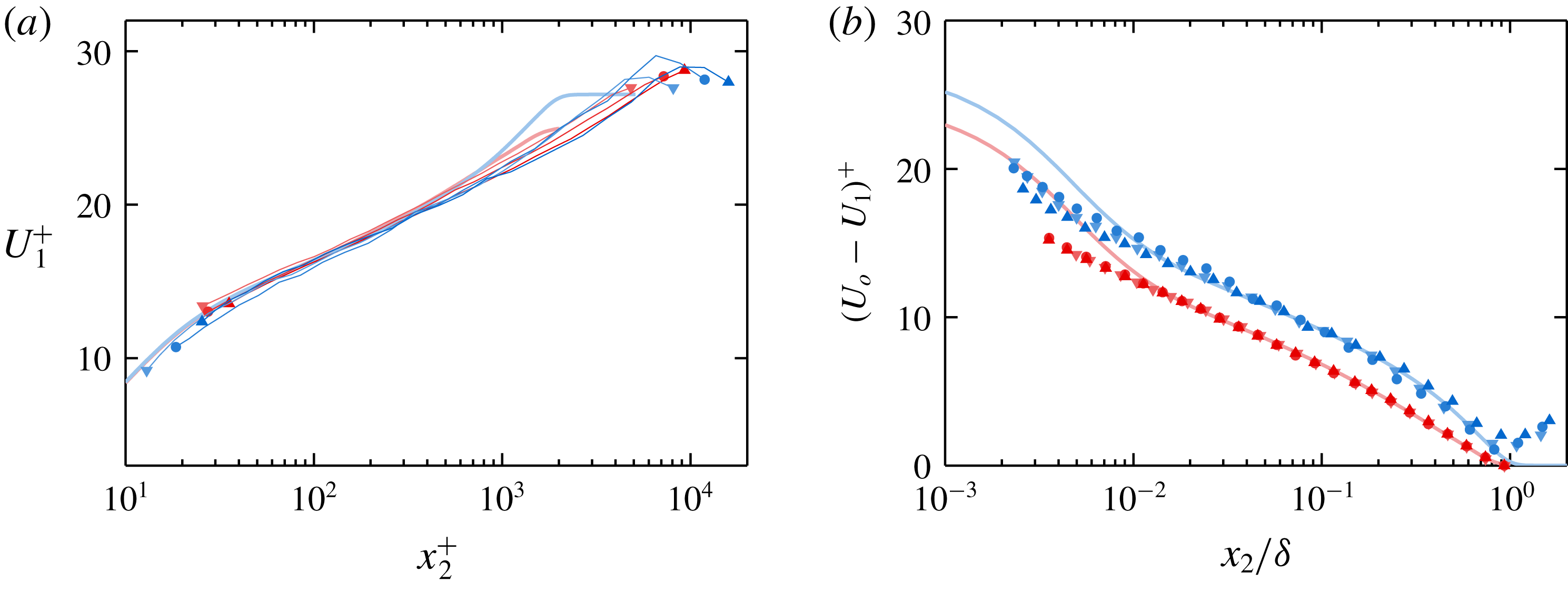
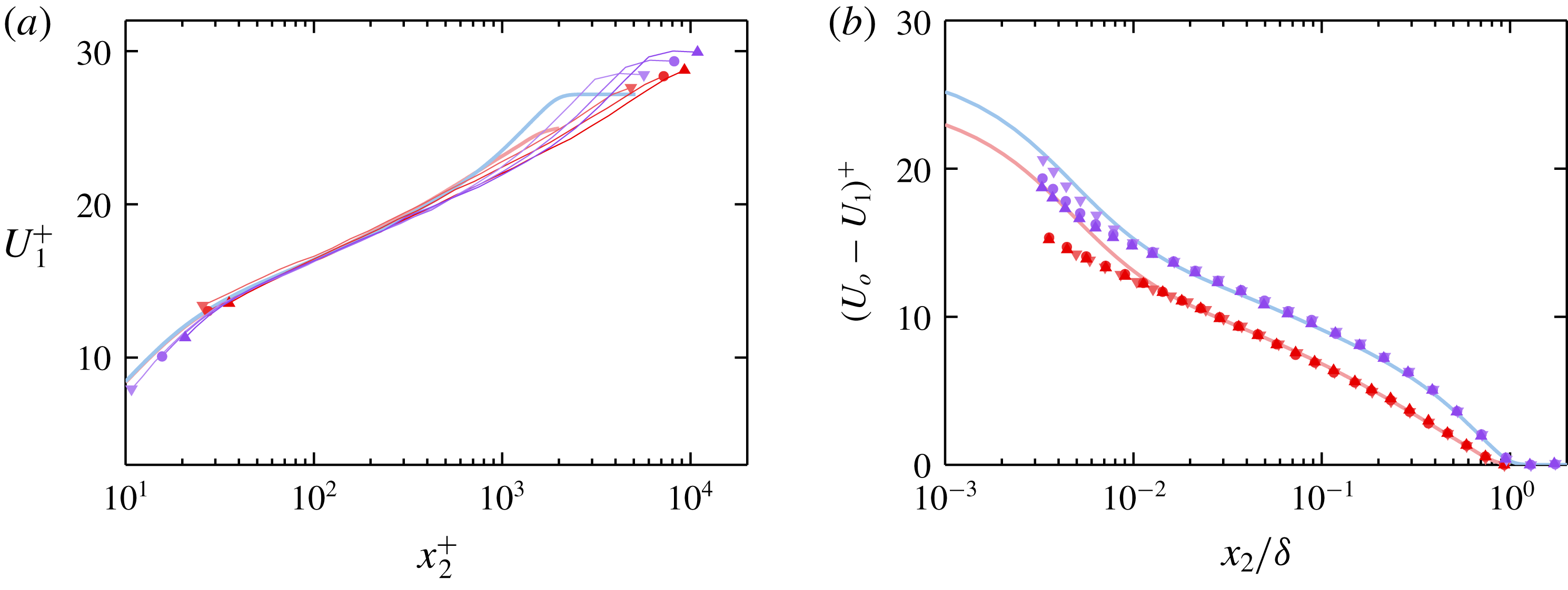
Figures 3(a) and 3(b) show the mean streamwise velocity
 $U_{1}$
in log-law and defect form, respectively. As noted in § 2.5,
 $U_{\unicode[STIX]{x1D70F}}$
is determined for the boundary layer by fitting the measured points to the composite profile of Chauhan et al. (Reference Chauhan, Monkewitz and Nagib2009) with a von Kármán constant
 $\unicode[STIX]{x1D705}=0.39$
and an intercept
 $B=4.3$
. Thus, agreement between the boundary layer cases and the boundary layer DNS of Sillero et al. (Reference Sillero, Jiménez and Moser2013) in the log layer is essentially prescribed. It is for this reason that the exact slopes of the profiles are not compared herein. Plotting the mean velocity in defect form, as in figure 3(b), reveals slight departures from canonical behaviour in the FPF boundary layer cases. For the purposes of this plot, the boundary layer free-stream velocity
 $U_{o}$
is chosen to force the log-law portions of each curve to lie on the expected ZPG boundary layer curve. This reveals that the two lower-
 $Re_{\unicode[STIX]{x1D70F}}$
boundary layer measurements show good agreement in the wake with the DNS of Sillero et al. (Reference Sillero, Jiménez and Moser2013) out to
 $x_{2}/\unicode[STIX]{x1D6FF}\approx 0.8$
, at which point
 $U_{1}$
reaches a maximum and begins to decrease. In addition to exhibiting the same local maxima in
 $U_{1}$
, the wake of the highest-
 $Re_{\unicode[STIX]{x1D70F}}$
boundary layer case is also slightly weaker than that of a canonical ZPG boundary layer wake. In spite of these departures from the expected
 $U_{1}$
profile shape, the turbulence statistics shown in the figures that follow (i.e. figures 4–11) show close agreement with the boundary layer DNS as well as with the (lower-
 $Re_{\unicode[STIX]{x1D70F}}$
) measurements collected at the HRNBLWT (shown in figures 15–19 in appendix A), even for
 $x_{2}/\unicode[STIX]{x1D6FF}_{99}>1$
. The present pipe measurements are virtually indistinguishable from the DNS curve of Chin et al. (Reference Chin, Monty and Ooi2014) through the log layer and wake. Likewise, the HRNBLWT
 $U_{1}$
profiles shown in figure 15 in appendix A show very close agreement with the DNS curve of Sillero et al. (Reference Sillero, Jiménez and Moser2013).
(a) Mean streamwise velocity in log-law form. Experimental profiles plotted as solid lines capped by symbols for clarity. Symbols at start/end of each line correspond to table 1. (b) Mean streamwise velocity in defect form, with
 $U_{o}$
chosen for the boundary layer cases to force agreement (for illustrative purposes) with log law (see text for details).

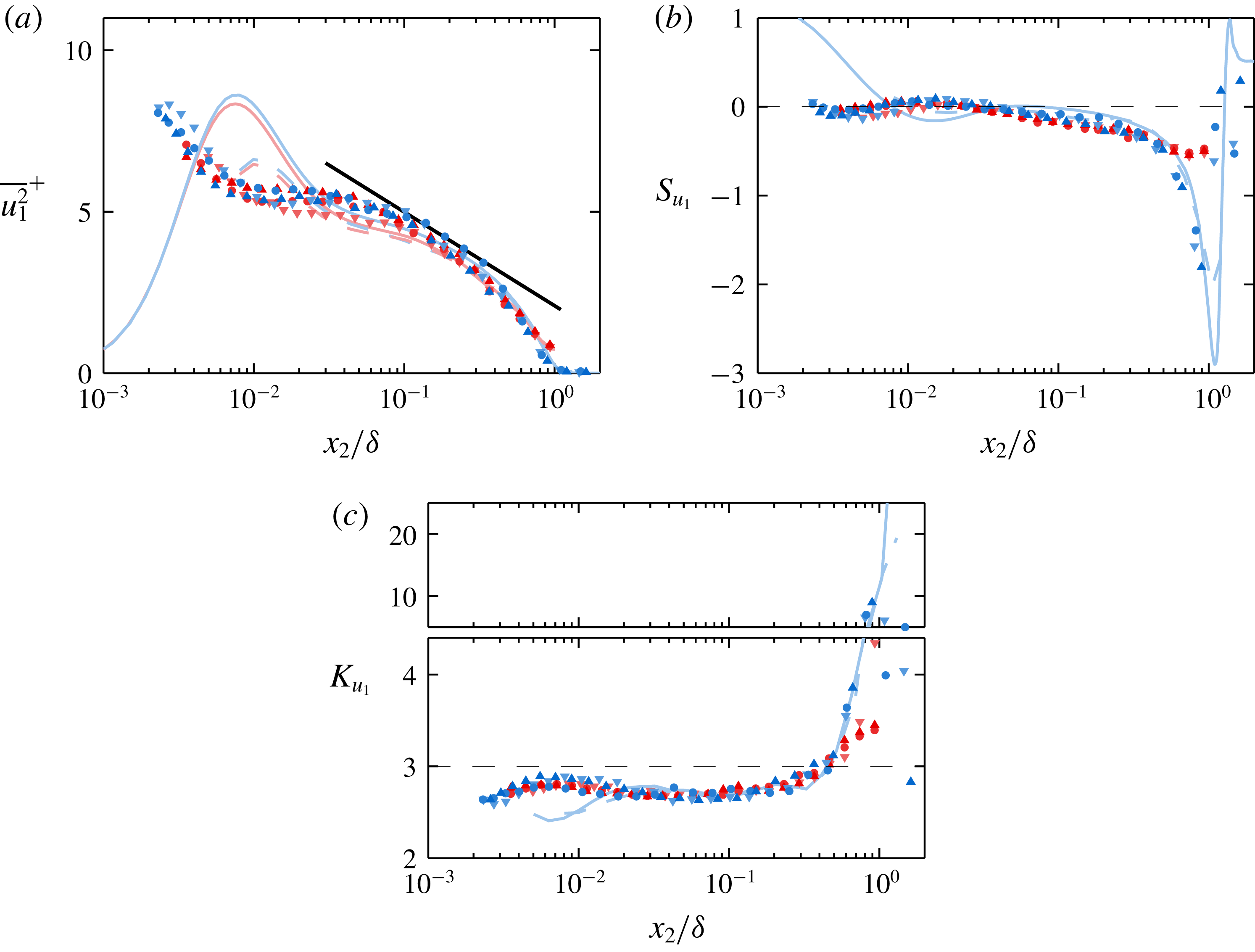
Figures 4(a), 4(b), and 4(c), respectively show the variance, skewness coefficient and kurtosis coefficient profiles of the fluctuating streamwise velocity
 $u_{1}$
for all present data and DNS. Apart from the expected difference in
 $\overline{u_{1}^{2}}^{+}$
near
 $x_{2}/\unicode[STIX]{x1D6FF}\approx 1$
, the
 $u_{1}$
variance profiles do not exhibit any systematic differences that are distinguishable with the present dataset. The similarity between the
 $\overline{u_{1}^{2}}^{+}$
profiles of the two flows is in agreement with Monty et al. (Reference Monty, Hutchins, Ng, Marusic and Chong2009), who presented streamwise velocity statistics up to the fourth order for pipe, channel and boundary layer flows. The HRNBLWT
 $u_{1}$
variance profiles, shown in figure 16(a) in appendix A, are also very similar in shape to the pipe profiles, although they do indicate that the boundary layer features slightly higher
 $u_{1}$
variance than the pipe over the range
 $0.3\gtrsim x_{2}/\unicode[STIX]{x1D6FF}\gtrsim 0.8$
. The difference being slight, however, means that this conclusion is particularly sensitive to the choice of outer length scale for the boundary layer. Still, it will be shown below that the enstrophy and the other components of the Reynolds stress tensor are all higher in the boundary layer than the pipe over approximately the same range.
(a–c) Fluctuating streamwise velocity variance, skewness and kurtosis, respectively. Logarithmic line of Marusic et al. (Reference Marusic, Monty, Hultmark and Smits2013) (i.e.
 $\overline{u_{1}^{2}}/U_{\unicode[STIX]{x1D70F}}^{2}=1.95-1.26\log (x_{2}/\unicode[STIX]{x1D6FF}_{99})+\log (1.15)$
) included in (a) for reference (note the additional
 $\log (1.15)$
constant accounts for differing definitions of
 $\unicode[STIX]{x1D6FF}$
). The dashed lines in (b) and (c) represent the Gaussian values of the plotted statistics.

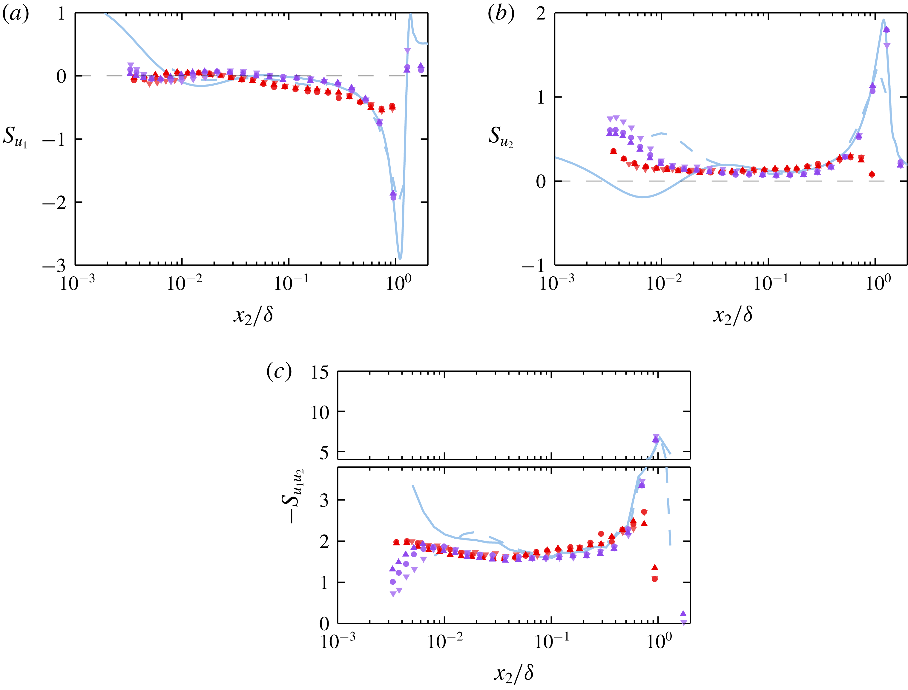
The streamwise velocity skewness coefficient profiles of the pipe and boundary layer are very similar from the wall until at least
 $x_{2}/\unicode[STIX]{x1D6FF}\approx 0.5$
. The profiles of both flows grow more negative at a rate that is approximately logarithmic across the sub-domain where the mean velocity is logarithmic. Monty et al. (Reference Monty, Hutchins, Ng, Marusic and Chong2009) also observed this similarity out to
 $x_{2}/\unicode[STIX]{x1D6FF}\approx 0.5$
, but remarked that ‘it could be argued that the boundary layer skewness exhibits a slightly different trajectory for
 $x_{2}^{+}\gtrsim 200$
’. Indeed, the boundary layer
 $u_{1}$
exhibits (on average) slightly less negative skewness than the pipe in the vicinity of
 $x_{2}/\unicode[STIX]{x1D6FF}\approx 0.1$
. The same is clearly true of the boundary layer data acquired in the HRNBLWT, as shown in figure 17 in appendix A. This difference is part of a general trend: the boundary layer exhibits higher variance and probability density functions that are less dominated by extreme events for most measured quantities near the outer edge of the log layer/wallward edge of the wake. It is surmised in § 5 that this results (at least in part) from the difference between intermittency associated with the turbulent/non-turbulent interface (TNTI) in the boundary layer and that associated with the turbulent/quiescent-core interface in the pipe.
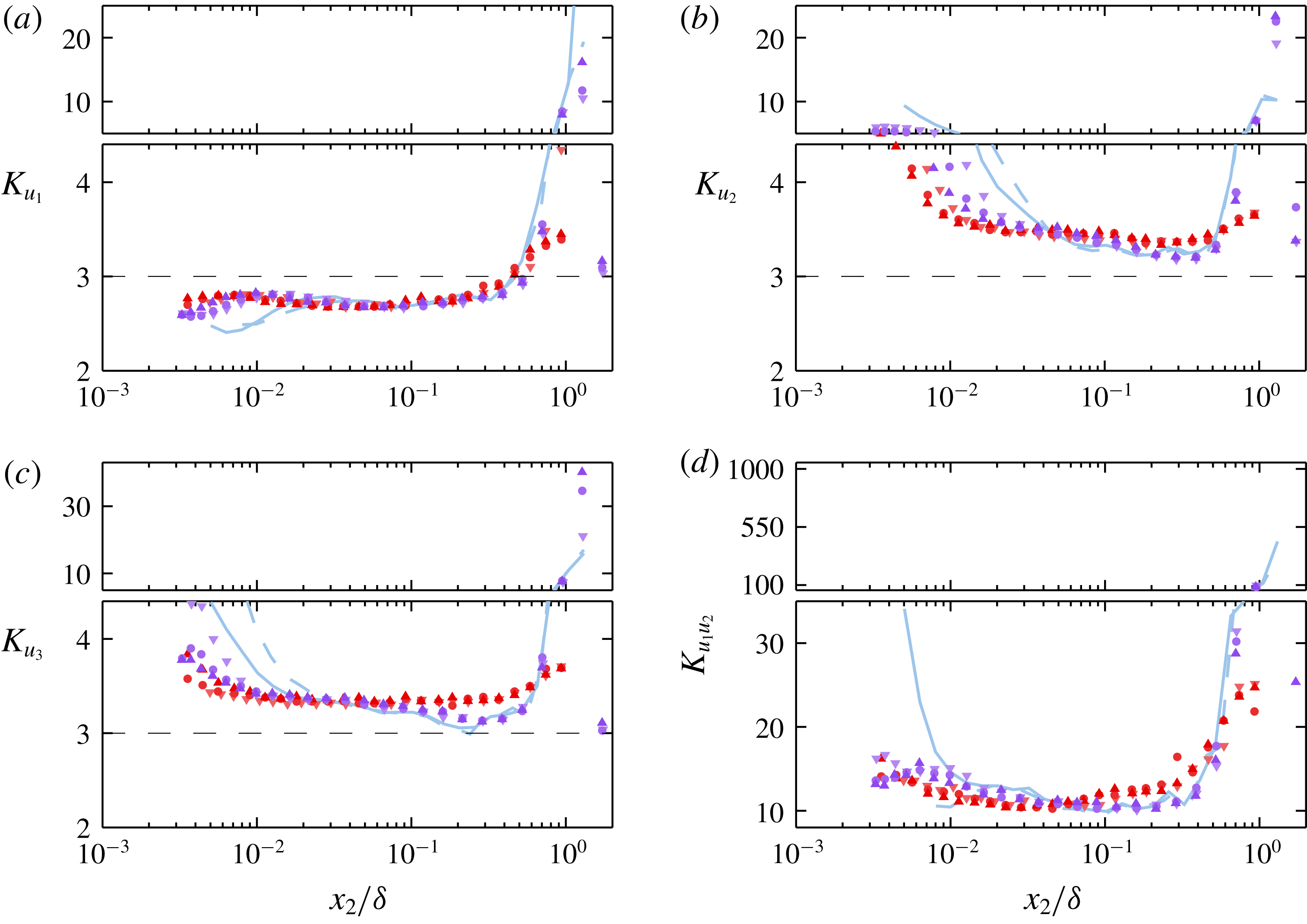
As with the skewness coefficient profiles, the pipe and boundary layer kurtosis profiles remain very similar moving outward from the wall until the emergence of a super-Gaussian peak in the wake of the boundary layer that far exceeds the more modest peak in the pipe (see figure 4
c). The HRNBLWT measurements, shown in figure 18 in appendix A, suggest that the boundary layer kurtosis is slightly lower than that of the pipe in the range
 $0.3\gtrsim x_{2}/\unicode[STIX]{x1D6FF}\gtrsim 0.5$
. Again, this is consistent with the differences between the intermittency in the pipe and boundary layer. Both profile sets remain sub-Gaussian from the nearest wall measured points until approximately
 $0.5\unicode[STIX]{x1D6FF}$
. The pipe centreline kurtosis is higher in the lowest-
 $Re_{\unicode[STIX]{x1D70F}}$
case than the two higher-
 $Re_{\unicode[STIX]{x1D70F}}$
cases. This higher value is observed individually by all sub-arrays, and at a position where the time-record length exceeded 25 000 radius turnover times. Thus, it is unlikely that this observation results from spurious probe behaviour or insufficient statistical convergence. As no two pipe measurements are collected at the same
 $Re_{\unicode[STIX]{x1D70F}}$
or sensor resolution, the cause of the difference in centreline kurtosis is left unclear.
3.2 Wall normal
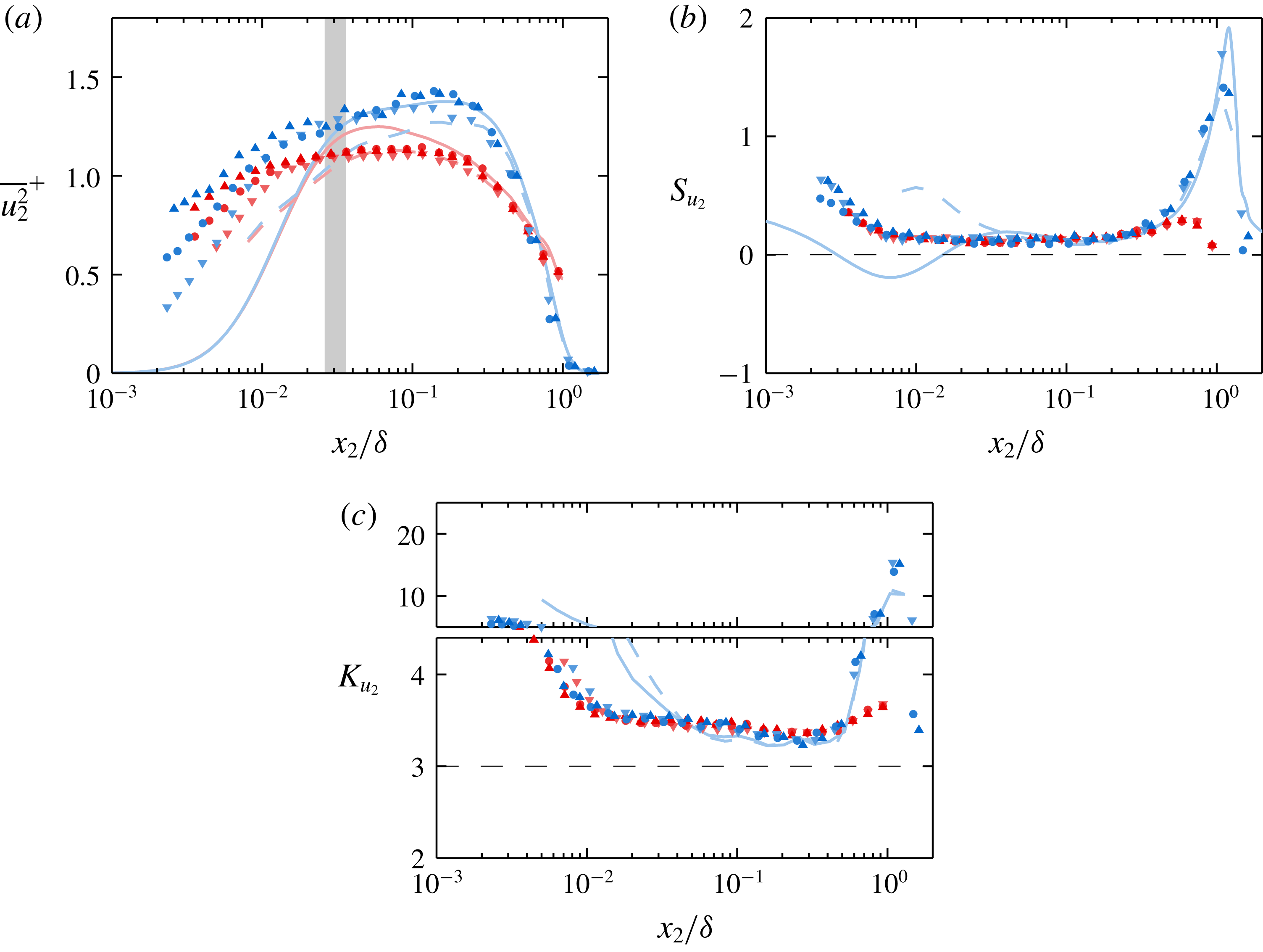
(a–c) Wall-normal velocity variance, skewness and kurtosis, respectively. Shaded region in (a) corresponds to the range of inner log-layer boundaries (i.e.
 $x_{2}^{+}\approx 2.6\sqrt{\unicode[STIX]{x1D6FF}^{+}}$
) for the present experiments. Dashed black lines indicate Gaussian values of the plotted statistics.

Figure 5 shows the variance, skewness and kurtosis profiles of the wall-normal velocity component. Based on the DNS-based synthetic probe predictions for the experimental data in figure 5(a), the wall-normal velocity variance is expected to suffer noticeable attenuation much farther from the wall than the streamwise velocity variance. Thus, while a slight positive slope is observed in the pipe
 $u_{2}$
variance across the domain where the mean velocity is logarithmic, it is unlikely that this trend would be observed in the absence of spatial filtering. Still, if either the absolute or proportional attenuation of the boundary layer and pipe
 $u_{2}$
signals are equal, the present data indicate that the
 $u_{2}$
variance differs between the two flows starting at least at the inner edge of the log layer. The same conclusion is reached via inspection of the HRNBLWT data, as shown in figure 16 in appendix A. According to both the experimental and DNS data, the difference in profiles is the most pronounced in the outer region
 $x_{2}/\unicode[STIX]{x1D6FF}\approx 0.2$
. At this location, the boundary layer case exhibits an outer peak that, according to Morrill-Winter et al. (Reference Morrill-Winter, Klewicki, Baidya and Marusic2015), continues to grow with increasing
 $Re_{\unicode[STIX]{x1D70F}}$
. The present pipe data does not exhibit an outer peak or any obvious trend with
 $Re_{\unicode[STIX]{x1D70F}}$
, and is of considerably lower magnitude than the boundary layer cases, in agreement with the findings of Jiménez & Hoyas (Reference Jiménez and Hoyas2008), which were observed at lower
 $Re_{\unicode[STIX]{x1D70F}}$
.
(a,b) Spanwise/azimuthal velocity variance and kurtosis profiles. Note the inclusion of the channel DNS variance profiles of Hoyas & Jiménez (Reference Hoyas and Jiménez2006) and Lee & Moser (Reference Lee and Moser2015), indicated by ‘


 $\overline{u_{3}^{2}}/U_{\unicode[STIX]{x1D70F}}^{2}=1.52-0.34\log (x_{2}/\unicode[STIX]{x1D6FF}_{99})$
for the boundary layer measurements and
 $\overline{u_{3}^{2}}/U_{\unicode[STIX]{x1D70F}}^{2}=1.11-0.42\log (x_{2}/\unicode[STIX]{x1D6FF})$
for the pipe measurements. Shaded region in (a) corresponds to the range of inner log-layer boundaries (i.e.
 $x_{2}^{+}\approx 2.6\sqrt{\unicode[STIX]{x1D6FF}^{+}}$
) for the present experiments. Dashed black line in (b) corresponds to Gaussian value the kurtosis.

As with the streamwise velocity, the pipe and boundary layer skewness and kurtosis profiles for
 $u_{2}$
(shown in figure 5
b,c) are very similar from the near wall to the onset of the wake region. The synthetic probe results predict that combined probe filtering/aliasing effects near the wall result in positive near-wall skewness, rather than the negative values reported by the fully resolved DNS. This effect is indeed observed in both the pipe and boundary layer experimental results. Once this effect becomes negligible, the DNS, pipe and boundary layer skewness profiles show very close agreement over the domain where the mean velocity is logarithmic. In all cases, the wall-normal fluctuations have an approximately constant skewness coefficient on this domain, varying only between 0.1 and 0.15. The pipe and boundary layer cases both exhibit a positive peak in the
 $u_{2}$
skewness in the wake region, although the magnitude of the boundary layer peak far exceeds that of the pipe. The existence of this skewness peak in the boundary layer is not altogether surprising given the non-zero skewness in the log layer and the presumed tendency of free-stream intermittency to increase the probability density of
 $u_{2}\approx 0$
. Although there is no source of truly non-turbulent ‘free stream’ in fully developed pipe flow, the intermittency associated with the varying boundary of the quiescent core (Kwon et al.
Reference Kwon, Philip, de Silva, Hutchins and Monty2014) would also presumably increase the probability density of
 $u_{2}\approx 0$
(as well as of
 $u_{3}\approx 0$
), and thus produce the observed outer peak in the pipe
 $u_{2}$
skewness profiles. Indeed, all of the velocity fluctuation skewness and kurtosis profiles presented herein exhibit a tendency to increase in magnitude as one moves outward from
 $x_{2}/\unicode[STIX]{x1D6FF}\approx 0.3$
, further supporting the existence of a quiescent core in the pipe. As with the
 $u_{1}$
component, the measurements of
 $S_{u_{2}}$
collected in the HRNBLWT (shown in figure 17 in appendix A) indicate that the boundary layer skewness is slightly more Gaussian (closer to zero) near the outer edge of the log layer/inner edge of the wake. Again, this is consistent with the differences shown in § 5 between the intermittency associated with the boundary layer TNTI and with the quiescent core in the pipe.
In contrast to the streamwise velocity fluctuations, the kurtosis of the
 $u_{2}$
fluctuations is super-Gaussian across the entire flow domain of both the pipe and the boundary layer. The kurtosis profiles of both flows exhibit an increase in magnitude as one moves from
 $x_{2}/\unicode[STIX]{x1D6FF}\approx 0.3$
towards the centreline, although the magnitude increase in the boundary layer far exceeds that of the pipe. While the difference between the
 $u_{2}$
skewness profiles of the two flows is detectable as close to the wall as
 $x_{2}/\unicode[STIX]{x1D6FF}\approx 0.35$
, the kurtosis profiles do not appear to rapidly diverge until
 $x_{2}/\unicode[STIX]{x1D6FF}\approx 0.55$
, which is close to the point at which the
 $u_{2}$
variance profiles intersect. Using the ‘intermittency factor’
 $\unicode[STIX]{x1D6FE}$
(defined as the time fraction of non-turbulent flow) to account for the effects of external intermittency, Schubauer (Reference Schubauer1954) found close agreement in the kinetic energy between the pipe and the turbulent portion of a boundary layer in the region above
 $x_{2}/\unicode[STIX]{x1D6FF}\approx 0.6$
. The author argued based on this agreement that the distribution of turbulent energy in a pipe and turbulent portion of a boundary layer are most likely the same in this region. The fact that the point at which the boundary layer and pipe
 $u_{2}$
variances are equal is approximately coincident with the point at which the kurtosis profiles begin to diverge is consistent with this hypothesis (at least for
 $x_{2}/\unicode[STIX]{x1D6FF}\gtrsim 0.6$
).
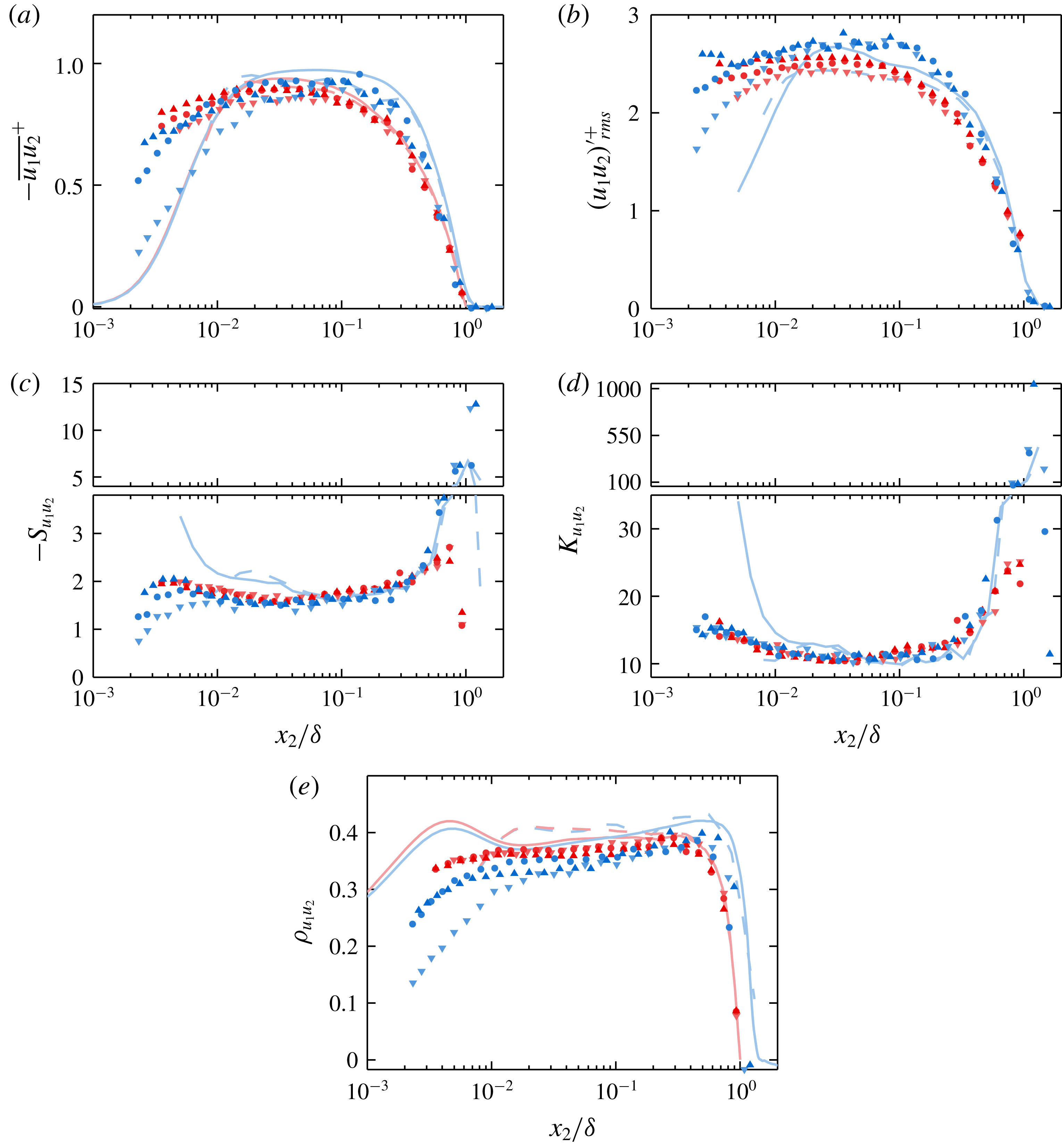
(a–e) Reynolds shear stress mean, r.m.s., skewness coefficient, kurtosis coefficient and correlation coefficient, respectively.

3.3 Spanwise/azimuthal
As the odd moments of the spanwise/azimuthal velocity are identically zero in both pipes and boundary layers in theory (and to within experimental error in actuality), figure 6 shows only the even-moment statistics of
 $u_{3}$
. Similar to
 $u_{2}$
, the
 $u_{3}$
boundary layer variance profiles show a sharp outer slope change, while the slope change in the pipe profiles is less pronounced. These slope changes occur at approximately
 $x_{2}/\unicode[STIX]{x1D6FF}\approx 0.3$
for both the DNS and experimental results, which is approximately coincident with the outer ‘bump’ feature in the
 $u_{2}$
variance profile, and is in agreement with the findings of Jiménez & Hoyas (Reference Jiménez and Hoyas2008) at lower
 $Re_{\unicode[STIX]{x1D70F}}$
. Further, this location is near the lower
 $x_{2}/\unicode[STIX]{x1D6FF}$
limit for turbulent/non-turbulent intermittency suggested by Chauhan, Philip & Marusic (Reference Chauhan, Philip and Marusic2014a
and Reference Chauhan, Philip, de Silva, Hutchins and Marusic2014b
). Thus, the ‘knee’ in the profile and subsequent rapid decay of
 $u_{3}$
variance is caused (at least in part) by an increasing time fraction of signal containing quasi-irrotational flow with near-zero spanwise velocity as one moves above
 $x_{2}/\unicode[STIX]{x1D6FF}\simeq 0.3$
.
That the
 $u_{3}$
variance is higher in magnitude (and features a different slope) in the boundary layer than in the pipe and channel below
 $0.3\unicode[STIX]{x1D6FF}$
is apparently a separate issue. Log lines of best fit computed from the present boundary layer and pipe
 $u_{3}$
variance data over the range
 $2.6\sqrt{\unicode[STIX]{x1D6FF}^{+}}<x_{2}^{+}<0.15\unicode[STIX]{x1D6FF}^{+}$
have slopes of
 $-0.34$
and
 $-0.42$
, respectively. The HRNBLWT
 $u_{3}$
variance measurements, shown in figure 16 in appendix A, feature a log-layer fit of
 $\overline{u_{3}^{2}}/U_{\unicode[STIX]{x1D70F}}^{2}=1.66-0.26\,\text{log}(x_{2}/\unicode[STIX]{x1D6FF})$
. If the difference between the pipe and boundary layer cases were predominantly related to flow geometry, one would expect the channel flow profile to closely resemble the boundary layer profile. Instead, the channel flow profile of Hoyas & Jiménez (Reference Hoyas and Jiménez2006) in figure 6 is virtually indistinguishable from the pipe flow profile of Chin et al. (Reference Chin, Monty and Ooi2014) at the same
 $Re_{\unicode[STIX]{x1D70F}}$
. The
 $Re_{\unicode[STIX]{x1D70F}}\approx 5200$
channel DNS of Lee & Moser (Reference Lee and Moser2015) is also shown in figure 6(a) for comparison. Although the higher
 $Re_{\unicode[STIX]{x1D70F}}$
DNS features slightly higher
 $u_{3}$
variance in the outer region than the
 $Re_{\unicode[STIX]{x1D70F}}\approx 2000$
pipe and channel DNS, it is still much closer to these cases than it is to the boundary layer DNS of Sillero et al. (Reference Sillero, Jiménez and Moser2013). Jiménez et al. (Reference Jiménez, Hoyas, Simens and Mizuno2010) suggested that the discrepancies between channel and boundary layer cases in both the
 $u_{2}$
and
 $u_{3}$
variance profiles are caused by higher pressure fluctuation root mean square (r.m.s.) in the boundary layer, resulting in an increased redistribution of the
 $u_{1}$
energy to the
 $u_{2}$
and
 $u_{3}$
components. This explanation is also appropriate for pipe flow as noted by Chin et al. (Reference Chin, Monty and Ooi2014), because the r.m.s. profiles of the pressure fluctuations in the pipe and channel also closely resemble one another, at least at
 $Re_{\unicode[STIX]{x1D70F}}\approx 1000$
. Jiménez et al. (Reference Jiménez, Hoyas, Simens and Mizuno2010) showed for a boundary layer and channel both at
 $Re_{\unicode[STIX]{x1D70F}}\approx 550$
that the difference in pressure r.m.s. in this region is due almost exclusively to the negative fluctuations, which are generally associated with the ‘cores’ of vortices. In support of this notion, it will be shown in §§ 4 and 5 that the boundary layer features higher mean enstrophy (at the resolved scales) and less quasi-irrotational flow in the same region.
Like the
 $u_{2}$
fluctuations, the
 $u_{3}$
fluctuations exhibit slightly super-Gaussian kurtosis throughout the entire flow domain of both pipes and boundary layers (see figure 6
b). The kurtosis for all three pipe profiles in the domain where the mean velocity is logarithmic remains constant at approximately 3.35 to within the scatter of the data. In contrast, all three boundary layer kurtosis profiles trend toward the Gaussian value of 3 with increasing distance from the wall within the log layer, moving from
 $\simeq 3.35$
to
 $\simeq 3.25$
. The local minimum of the boundary layer kurtosis profiles corresponds approximately to the location of the ‘knee’ in the variance profiles (see figure 6
a). The difference between the pipe and boundary layer
 $u_{3}$
kurtosis is also clear when using the HRNBLWT measurements as in figure 18(c) in appendix A. This feature, again, is consistent with the difference in the time fractions of ‘fully’ turbulent flow (as opposed to quiescent or non-turbulent) near the outer edge of the log layer that will be discussed further in § 5.
As is the case with
 $u_{2}$
fluctuations, the point at which the boundary layer and pipe
 $u_{3}$
variance profiles intersect is approximately coincident with the point at which the kurtosis profiles rapidly diverge, with both features occurring near
 $x_{2}/\unicode[STIX]{x1D6FF}\approx 0.6$
. Again, this is consistent with the hypothesis of Schubauer (Reference Schubauer1954) that the distribution of turbulent energy between the pipe and the turbulent patches of the boundary layer is the same over this region.
3.4 Reynolds shear stress
Owing in part to its strong dependence on probe alignment (Zimmerman et al.
Reference Zimmerman, Morrill-Winter and Klewicki2017), the mean Reynolds shear stress is one of the more difficult statistics to accurately measure. The magnitude of all present kurtosis profiles of the instantaneous
 $u_{1}u_{2}$
signal reveal its highly intermittent nature, and indicate that the mean value is composed of a delicate balance of instantaneous motions that often far exceed the magnitude of the mean in both directions. That said, the present mean Reynolds stress profiles in the boundary layer (see figure 7
a) do exhibit the expected outer region deviation from the pipe cases in the same region as the observed boundary layer ‘knees’ in both the
 $\overline{u_{2}^{2}}$
and
 $\overline{u_{3}^{2}}$
profiles. This difference is shown more clearly in the HRNBLWT measurements (cf. figure 16
d in appendix A).
The slightly higher mean Reynolds stress values in the outer region of the boundary layer in figure 7(a) are matched by slightly higher signal r.m.s. boundary layer profiles compared to the pipe profiles as shown in figure 7(b). In agreement with the findings of Morrill-Winter (Reference Morrill-Winter2016) and the computation from the available DNS fields, the Reynolds shear stress signal is negatively skewed across the entire flow domain with a coefficient of
 $S_{u_{1}u_{2}}\approx -1.6$
in the region where the mean velocity is logarithmic (see figure 7
c). The skewness and kurtosis profiles for the pipe experiments closely resemble those of the boundary layer out to
 $x_{2}/\unicode[STIX]{x1D6FF}\simeq 0.5$
. As with the constituent components
 $u_{1}$
and
 $u_{2}$
, the HRNBLWT measurements indicate that the
 $u_{1}u_{2}$
skewness and kurtosis magnitudes are slightly lower in the boundary layer than in the pipe near the outer edge of the log layer. This is also shown by the FPF measurements (at least in a mean sense), albeit less convincingly. This slight discrepancy is likely related to the departures from the canonical ZPG wake discussed in § 3.1.
The
 $(u_{1}u_{2})^{\prime }$
skewness reaches a negative peak in the wake regions of both the pipe and boundary layer. As with the skewness profiles of the constituent velocity components, the peak magnitude in the boundary layer far exceeds that of the pipe. As noted above, the instantaneous fluctuating
 $u_{1}u_{2}$
signal is characterized by extreme events, resulting in a kurtosis greater than 10 across the entire flow domain (see figure 7
d). The pipe and boundary layer kurtosis profiles appear to match one another everywhere except in the wake region. Here, a substantial increase in the pipe profiles is outpaced by an even more substantial peak in the boundary layer profiles.
The correlation coefficient
 $\unicode[STIX]{x1D70C}_{u_{1}u_{2}}$
is shown in figure 7(e). While the present experimental results are of lower magnitude than the synthetic experiment and DNS, a slight decrease in magnitude is expected with increasing
 $Re_{\unicode[STIX]{x1D70F}}$
. This decrease in magnitude is expected since (at least) the
 $u_{1}$
fluctuations are known to increase in strength with increasing
 $Re_{\unicode[STIX]{x1D70F}}$
(albeit slowly) in the region where the mean Reynolds shear stress remains close to
 $-U_{\unicode[STIX]{x1D70F}}^{2}$
. The correlation coefficient in the pipe remains fairly constant over the majority of the flow domain (in logarithmic space) before turning sharply toward zero, passing through
 $-0.3$
at
 $x_{2}/\unicode[STIX]{x1D6FF}\simeq 0.7$
. In contrast, the boundary layer correlation coefficient profiles slope gently away from zero for the majority of the flow domain before turning sharply toward zero, passing through
 $-0.3$
at
 $x_{2}/\unicode[STIX]{x1D6FF}_{99}\simeq 0.8{-}1$
.
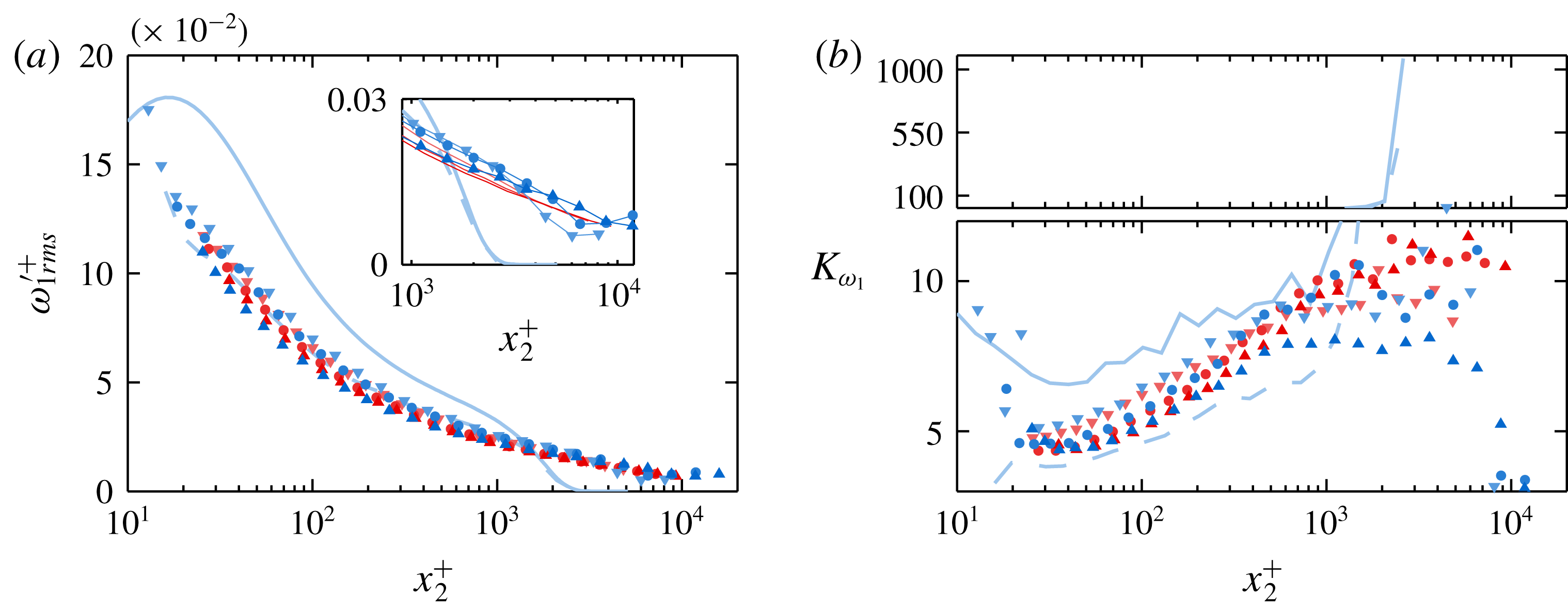
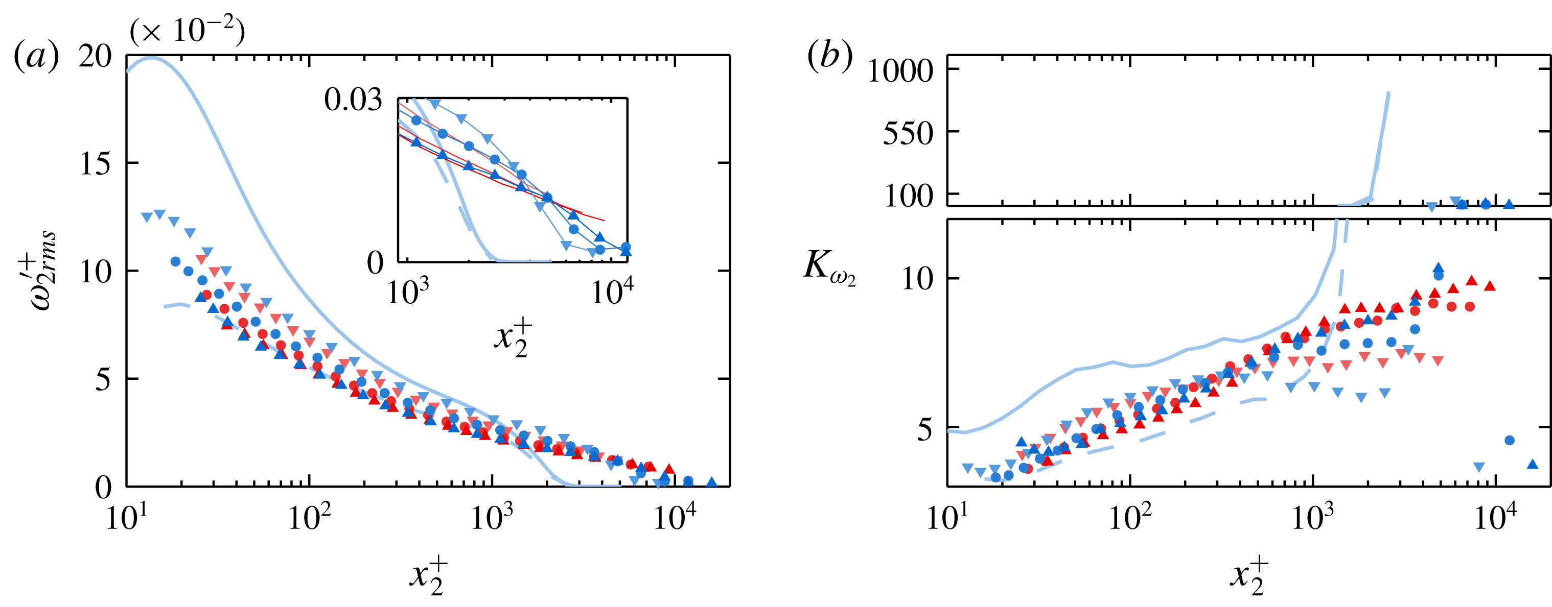
(a) Inner-normalized streamwise vorticity r.m.s. and (b) kurtosis coefficient profiles. Inset to (a) depicts pipe profiles as lines without symbols and boundary layer profiles as symbols with lines for clarity.

(a) Inner-normalized wall-normal vorticity r.m.s. and (b) kurtosis coefficient profiles. Inset to (a) depicts pipe profiles as lines without symbols and boundary layer profiles as symbols with lines for clarity.

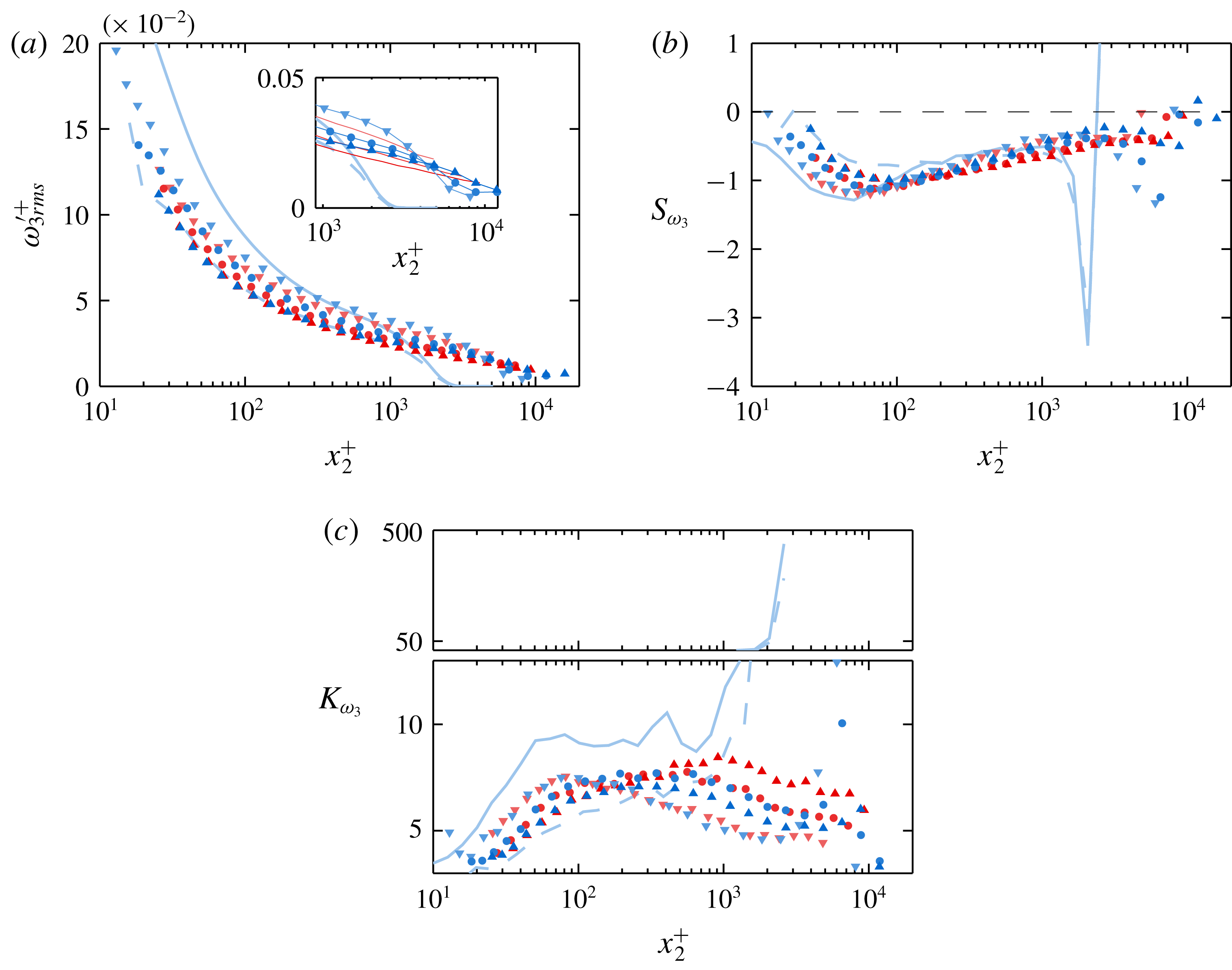
(a) Inner-normalized spanwise/azimuthal vorticity r.m.s., (b) skewness coefficient and (c) kurtosis coefficient profiles. Inset to (a) depicts pipe profiles as lines without symbols and boundary layer profiles as symbols with lines for clarity.

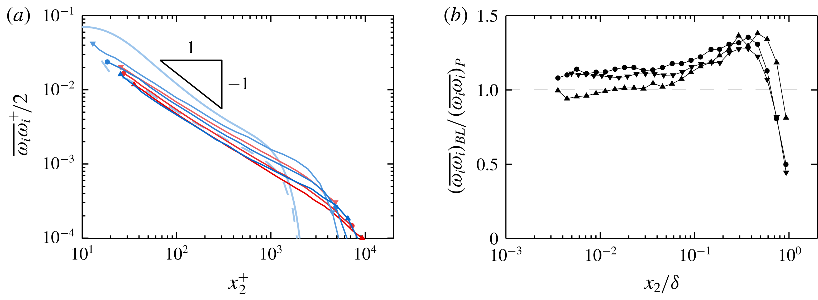
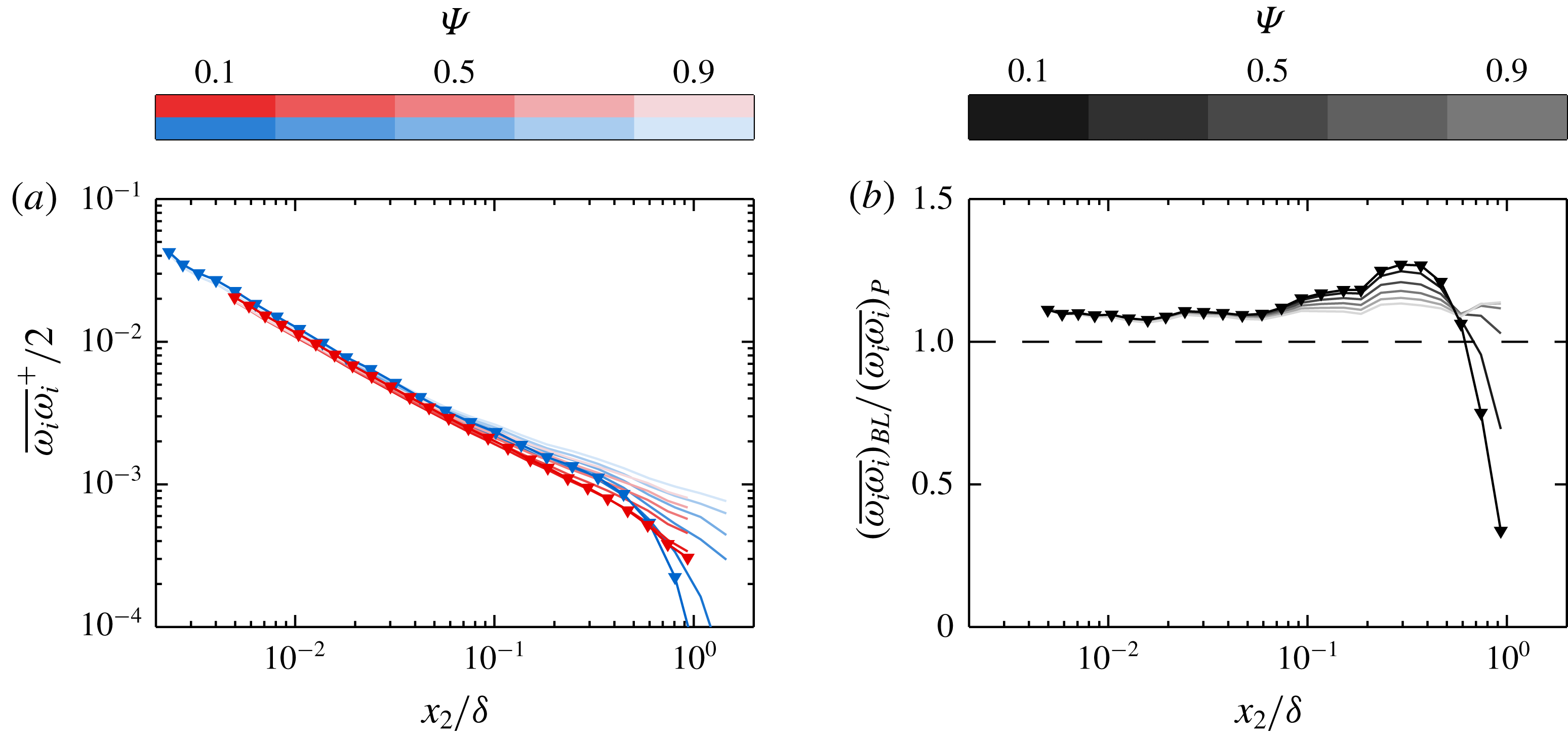
(a) Inner-normalized turbulence enstrophy profiles plotted as solid lines capped by symbols for clarity. Symbols at start/end of each line correspond to table 1. (b) Ratio of turbulence enstrophy between boundary layers and pipes of approximately matched
 $Re_{\unicode[STIX]{x1D70F}}$
and spatial resolution. Symbol shape corresponds to spatial resolution in accordance with the trend established in table 1.

4 Vorticity
This section presents statistics of all three components of vorticity, as well as the mean enstrophy
 $(1/2)\overline{\unicode[STIX]{x1D714}_{i}\unicode[STIX]{x1D714}_{i}}$
. Where the velocity statistics elucidate the distribution of motions contributing to the kinetic energy of the turbulence, the vorticity statistics describe (to a close approximation) the distribution of contributions to the dissipation of turbulence kinetic energy. Furthermore, the distribution of the spanwise/azimuthal vorticity describes the motions which underlie the slope of the mean velocity profile (i.e. since
 $\unicode[STIX]{x1D6FA}_{3}\approx -\unicode[STIX]{x2202}U_{1}/\unicode[STIX]{x2202}x_{2}$
).
Figures 8 through 10 show statistics of the streamwise, wall-normal and spanwise/azimuthal components of vorticity, respectively. Each component exhibits similar features, including an outer ‘bump’ in the boundary layer r.m.s. (at a location that is coincident with ‘bumps’ in the Reynolds stresses described above) and universal super-Gaussian kurtosis.
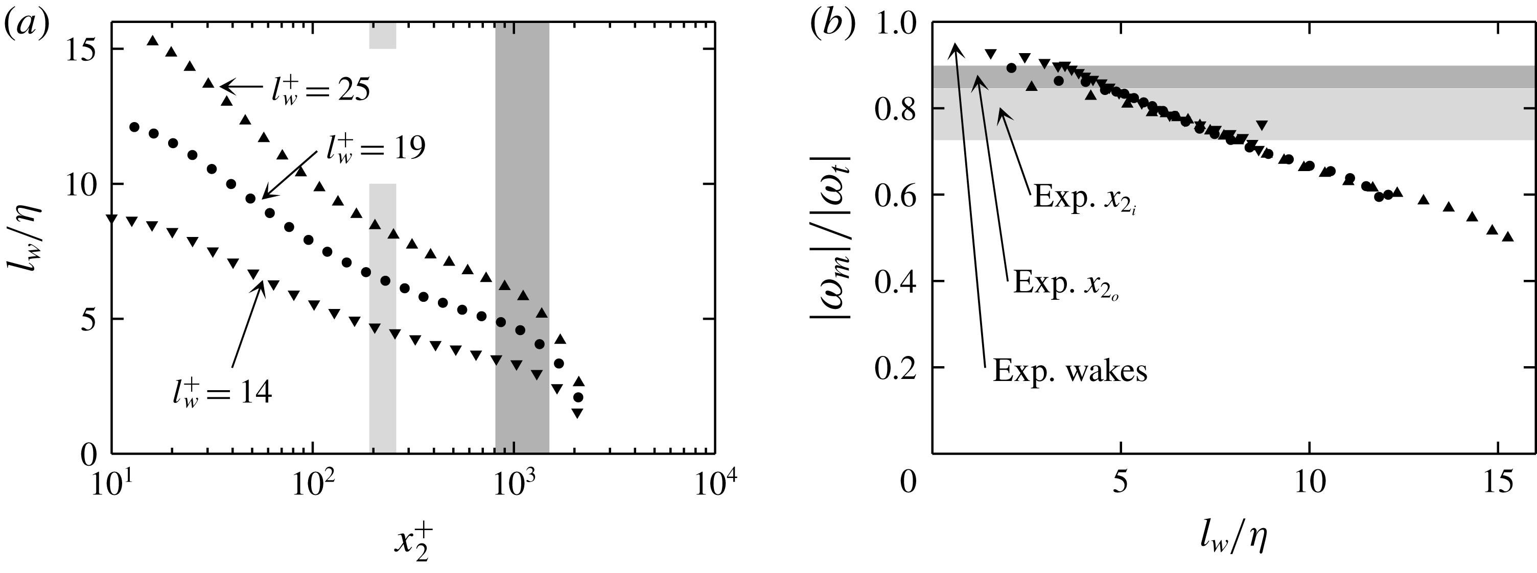
The fraction of boundary layer vorticity r.m.s. that is resolved by the present measurement technique may be predicted via the ‘synthetic’ experiment described briefly in § 2.5 and in detail in Zimmerman et al. (Reference Zimmerman, Morrill-Winter and Klewicki2017). The effects of physical scale, probe geometry and data reduction method are reproduced in a DNS volume by using the known velocity fields and model calibration functions to generate synthetic sensor ‘voltages’, which are then reduced to velocities and velocity gradients according to the process outlined in § 2.4. The ratio of ‘measured’ to ‘true’ vorticity predicted by the synthetic experiment is reported for the three resolution cases in figure 20 in appendix B. The effects of spatial resolution on the vorticity r.m.s. and kurtosis values, as predicted by the synthetic experiment, are given herein by the dashed light-blue lines in each plot. This synthetic case corresponds to the least-resolved physical experimental cases (see table 1), and so all the experimental data are expected to approximately lie between the DNS computations and the synthetic experimental curve in the absence of effects not captured by the synthetic experimental model.
When both spatial resolution and
 $Re_{\unicode[STIX]{x1D70F}}$
are matched, the streamwise vorticity r.m.s. profiles of the pipe and boundary layer closely resemble one another. Zimmerman et al. (Reference Zimmerman, Morrill-Winter and Klewicki2017) argued that the variability among vorticity r.m.s. profiles (of all three components) for unmatched cases is primarily a function of spatial resolution, and should not be confused for a Reynolds number trend. This argument was based on the observed agreement between two physical experimental ZPG cases with matched resolution but disparate Reynolds numbers, as well as agreement between physical and synthetic experimental results across a range of spatial resolutions.
The outer boundary condition for all three vorticity components differs between the pipe and boundary layer cases in that the pipe r.m.s. profiles do not go to zero. Thus, the change in concavity observed in the boundary layer DNS profiles (see figures 8 a, 9 a and 10 a) in the wake region is not expected to exist, at least to the same degree, in the pipe profiles. Although this result is somewhat obfuscated by non-zero free-stream r.m.s. in the boundary layer cases, it is still visible in the insets of figures 8(a), 9(a) and 10(a). The pipe profiles are shown in the insets as lines without symbols for clarity.
With the exception of the highest
 $Re_{\unicode[STIX]{x1D70F}}$
boundary layer case, both the pipe and boundary layer kurtosis profiles increase across the flow domain. As the streamwise component of vorticity is composed exclusively of cross-stream gradients of cross-stream velocity components, any imbalance in the measurement of these sensitive velocity components between two sub-arrays may result in signal contamination. Even a slight increase in the denominator of the kurtosis coefficient due to contamination may be the cause of not only the flattening of the highest
 $Re_{\unicode[STIX]{x1D70F}}$
boundary layer kurtosis profile, but also the lack of outer peaks in the two higher-
 $Re_{\unicode[STIX]{x1D70F}}$
boundary layer kurtosis profiles.
The boundary layer
 $\unicode[STIX]{x1D714}_{2}$
r.m.s. profiles shown in figure 9(a) clearly exhibit the expected change in concavity in the wake region while the pipe profiles do not. The
 $\unicode[STIX]{x1D714}_{2}$
kurtosis profiles are very similar to the
 $\unicode[STIX]{x1D714}_{1}$
kurtosis profiles for both the pipe and boundary layer cases, except that the predicted outer peak in the boundary layer profiles is present in the experimental results. The
 $\unicode[STIX]{x1D714}_{2}$
kurtosis of the boundary layer cases is also less than that of the pipe in the outer region, a feature which was also observed in at least the
 $u_{2}$
and
 $u_{3}$
component kurtosis profiles over approximately the same wall-normal domain. Again, this is related to the differing properties of intermittency associated with the TNTI in the boundary layer and the quiescent core in the pipe.
As with the two zero-mean vorticity components (i.e.
 $\unicode[STIX]{x1D714}_{1}$
and
 $\unicode[STIX]{x1D714}_{2}$
), the pipe and boundary layer
 $\unicode[STIX]{x1D714}_{3}$
vorticity r.m.s. profiles closely resemble each other with the exception of the change of concavity observed in the boundary layer wake. The spanwise/azimuthal vorticity fluctuations for both the pipe and boundary layer cases are skewed with the same sign as the mean across the entire flow domain (see figure 10
b). This is reflective of the existence of spatially concentrated regions of strong
 $\unicode[STIX]{x2202}U_{1}/\unicode[STIX]{x2202}x_{2}$
shear (e.g. as observed by Meinhart & Adrian (Reference Meinhart and Adrian1995)). The pipe skewness profiles in particular appear to follow a steady logarithmic curve toward zero, but with a slope that is too shallow to intersect zero at the centreline. An abrupt turn toward zero skewness is observed in all three pipe profiles between the two centremost points at
 $0.74\unicode[STIX]{x1D6FF}$
and
 $0.93\unicode[STIX]{x1D6FF}$
that hints at the path taken by the curve to satisfy the symmetry condition of
 $S_{\unicode[STIX]{x1D714}_{3}}=0$
at the centreline. Continuing the trend observed in a number of third- and fourth-order statistics of other quantities, the boundary layer
 $\unicode[STIX]{x1D714}_{3}$
skewness is of smaller magnitude than that of the pipe near the outer edge of the log layer.
The
 $\unicode[STIX]{x1D714}_{3}$
kurtosis profiles, shown in figure 10(c), exhibit qualitatively different behaviour than the two zero-mean vorticity component kurtosis profiles. Where the
 $\unicode[STIX]{x1D714}_{1}$
and
 $\unicode[STIX]{x1D714}_{2}$
signals become increasingly dominated by large fluctuations as one moves away from the wall (kurtosis increasing gradually from 5 to 10), the
 $\unicode[STIX]{x1D714}_{3}$
kurtosis profiles exhibit no such monotonic increase. The slight trends in kurtosis profiles observed for the different
 $Re_{\unicode[STIX]{x1D70F}}$
cases are likely related to changes in spatial resolution. With the exception of the highest-
 $Re_{\unicode[STIX]{x1D70F}}$
boundary layer case, the pipe and boundary layer kurtosis profiles track each other closely.
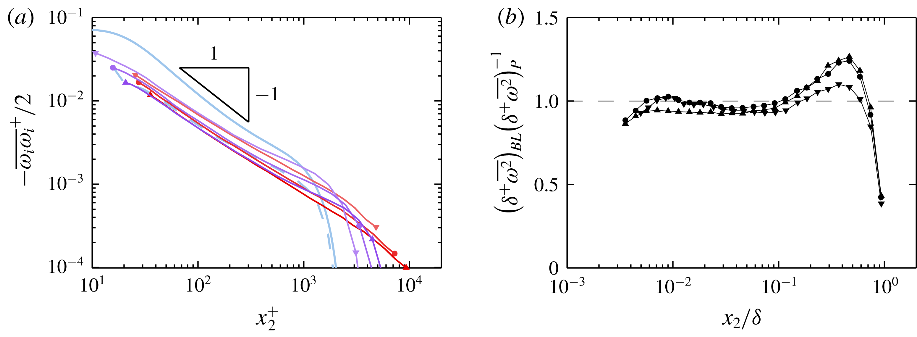
Figure 11(a) shows the mean turbulence enstrophy,
 $(1/2)\overline{\unicode[STIX]{x1D714}_{i}\unicode[STIX]{x1D714}_{i}}$
, on a logarithmic scale. Since the enstrophy is related to the turbulence dissipation rate
 $\overline{\unicode[STIX]{x1D716}}$
by
 $\overline{\unicode[STIX]{x1D716}}\approx \unicode[STIX]{x1D708}\overline{\unicode[STIX]{x1D714}_{i}\unicode[STIX]{x1D714}_{i}}$
, the classical
 $-1$
power-law slope (based on equality of production and dissipation, e.g. see Townsend (Reference Townsend1976)) is also included in figure 11(a) for reference. Figure 11(b) shows the ratio of the enstrophy profiles of the boundary layer and pipe cases with matched
 $Re_{\unicode[STIX]{x1D70F}}$
and spatial resolution. The outer peaks observed in the enstrophy ratio profiles coincide with the change-of-concavity discussed above in the context of figures 8 through 10 as well as the outer ‘bumps’ in the boundary layer
 $u_{2}$
and
 $u_{3}$
variance profiles relative to those of the pipe. Figure 11 is replotted as figure 19 in appendix A using the HRNBLWT measurements in place of the FPF measurements. The same peak in the enstrophy ratio is also clearly visible in figure 19(b), although the region where the ratio departs from unity is more clearly discernible as
 $0.1\lesssim x_{2}/\unicode[STIX]{x1D6FF}\lesssim 0.7$
.
As noted above in § 3.3, the cross-stream velocity variances and enstrophy are linked through the pressure root mean square. Increased levels of mean enstrophy are associated with stronger negative pressure fluctuations (which were indeed observed by Jiménez et al. (Reference Jiménez, Hoyas, Simens and Mizuno2010)), while increased pressure r.m.s. is linked to increased redistribution of
 $u_{1}$
energy to
 $u_{2}$
and
 $u_{3}$
through the pressure–strain redistribution term in the Reynolds stress transport equations (e.g. see Tennekes & Lumley (Reference Tennekes and Lumley1972)). The differences in mean enstrophy are also indicative of increased levels of viscous dissipation of turbulence in the boundary layer wake relative to the pipe wake, in agreement with El Khoury et al. (Reference El Khoury, Schlatter, Noorani, Fischer, Brethouwer and Johansson2013) wherein channel, pipe, and ZPG boundary layer DNS results are compared at
 $Re_{\unicode[STIX]{x1D70F}}\approx 1000$
. The following section shows that the difference in enstrophy levels observed in the pipe and boundary layer are related to the differing time-fractions of highly turbulent flow. These time fractions are themselves a product of the properties of the TNTI in the boundary layer and the quiescent-core boundary in the pipe.
5 Intermittency
Two overarching features of the r.m.s., skewness and kurtosis profiles are shown in § 3 and § 4 to consistently differentiate between pipe and boundary layer flow: outer magnitude peaks in the boundary layer skewness and kurtosis cases that emerge at
 $x_{2}/\unicode[STIX]{x1D6FF}\approx 0.5$
; and higher r.m.s./lower skewness and kurtosis magnitude of boundary layer quantities over a domain roughly spanning
 $0.1\lesssim x_{2}/\unicode[STIX]{x1D6FF}\lesssim 0.5$
. The emergence of an outer peak in the kurtosis profiles of boundary layer statistics has long been understood to be related to turbulent/non-turbulent intermittency in the boundary layer. Early studies of this phenomenon even used the departure of the
 $u_{1}$
kurtosis from the Gaussian value as a measure of intermittency (Klebanoff Reference Klebanoff1955). Some profile features that are typically understood to be a consequence of intermittency, however, are also observed (albeit to a lesser degree) in the present pipe cases. Indeed, all of the third and fourth order velocity statistics presented herein for the pipe trend away from Gaussian values in the outer flow region. Recently, Kwon et al. (Reference Kwon, Philip, de Silva, Hutchins and Monty2014) have shown that channel flows contain in their wake a region of nearly uniform momentum, or a ‘quiescent core’, which has characteristics similar to those of the boundary layer free stream. The role of these quasi-‘non-turbulent’ patches is thus of interest. The aim of this section is to identify differences in the structure and prevalence of flow having characteristics reminiscent of the boundary layer free stream – namely irrotationality and unidirectionality.
As the vorticity signal is not fully resolved by the present measurement technique (see appendix B for details), it is not possible to identify portions of the signal that are strictly irrotational. Instead, a range of thresholds for instantaneous enstrophy,
 $(1/2)\tilde{\unicode[STIX]{x1D714}}_{i}\tilde{\unicode[STIX]{x1D714}}_{i}$
, are used to identify ‘irrotational’ or ‘quasi-irrotational’ flow. The conclusions drawn from these data are then shown to be independent of the threshold level over the range employed. As shown in figure 11, the enstrophy roughly decreases as
 $x_{2}^{-1}$
from
 $x_{2}^{+}\gtrsim 30$
to
 $x_{2}/\unicode[STIX]{x1D6FF}\lesssim 0.5$
. In effect, the mean turbulence enstrophy at, say,
 $x_{2}/\unicode[STIX]{x1D6FF}=0.1$
for
 $Re_{\unicode[STIX]{x1D70F}}\approx 10\,000$
is therefore roughly half that at the same position for
 $Re_{\unicode[STIX]{x1D70F}}\approx 5000$
. Since the present intermittency analysis is primarily focused on the outer region of the flow, it is therefore logical to define a threshold relative to the enstrophy at some point in the outer region for each
 $Re_{\unicode[STIX]{x1D70F}}$
case rather than, for example, one fixed in viscous units. For the purposes of the present analysis, the threshold enstrophy is expressed relative to the mean enstrophy at
 $x_{2}^{\ast }$
, the location where the pipe and boundary layer enstrophy values are equal (
 $x_{2}^{\ast }/\unicode[STIX]{x1D6FF}\approx 0.7$
according to figure 11
b). The threshold level for each measurement may then be represented in terms of the coefficient
 $\unicode[STIX]{x1D6F9}$
, defined as follows:
 $$\begin{eqnarray}\displaystyle \unicode[STIX]{x1D6F9}=C_{\unicode[STIX]{x1D714}\unicode[STIX]{x1D714}}\left({\textstyle \frac{1}{2}}\overline{\unicode[STIX]{x1D714}_{i}(x_{2}^{\ast })\unicode[STIX]{x1D714}_{i}(x_{2}^{\ast })}\right)^{-1}, & & \displaystyle\end{eqnarray}$$
where
 $C_{\unicode[STIX]{x1D714}\unicode[STIX]{x1D714}}$
is the actual threshold value in
 $\text{s}^{-2}$
.
Although the velocity measurements are less susceptible to attenuation in the outer region than the vorticity measurements, a range of thresholds will also be used to determine ‘unidirectionality’ to ensure independence of the conclusions from the chosen threshold level. The criterion for ‘unidirectionality’ is defined herein as the total velocity flow angle relative to the
 $x_{1}$
direction, which is calculated according to (5.2) below:
 $$\begin{eqnarray}\displaystyle \unicode[STIX]{x1D703}=\tan ^{-1}\left(\frac{\tilde{u} _{1}}{(\tilde{u} _{1}^{2}+\tilde{u} _{2}^{2}+\tilde{u} _{3}^{2})^{1/2}}\right). & & \displaystyle\end{eqnarray}$$
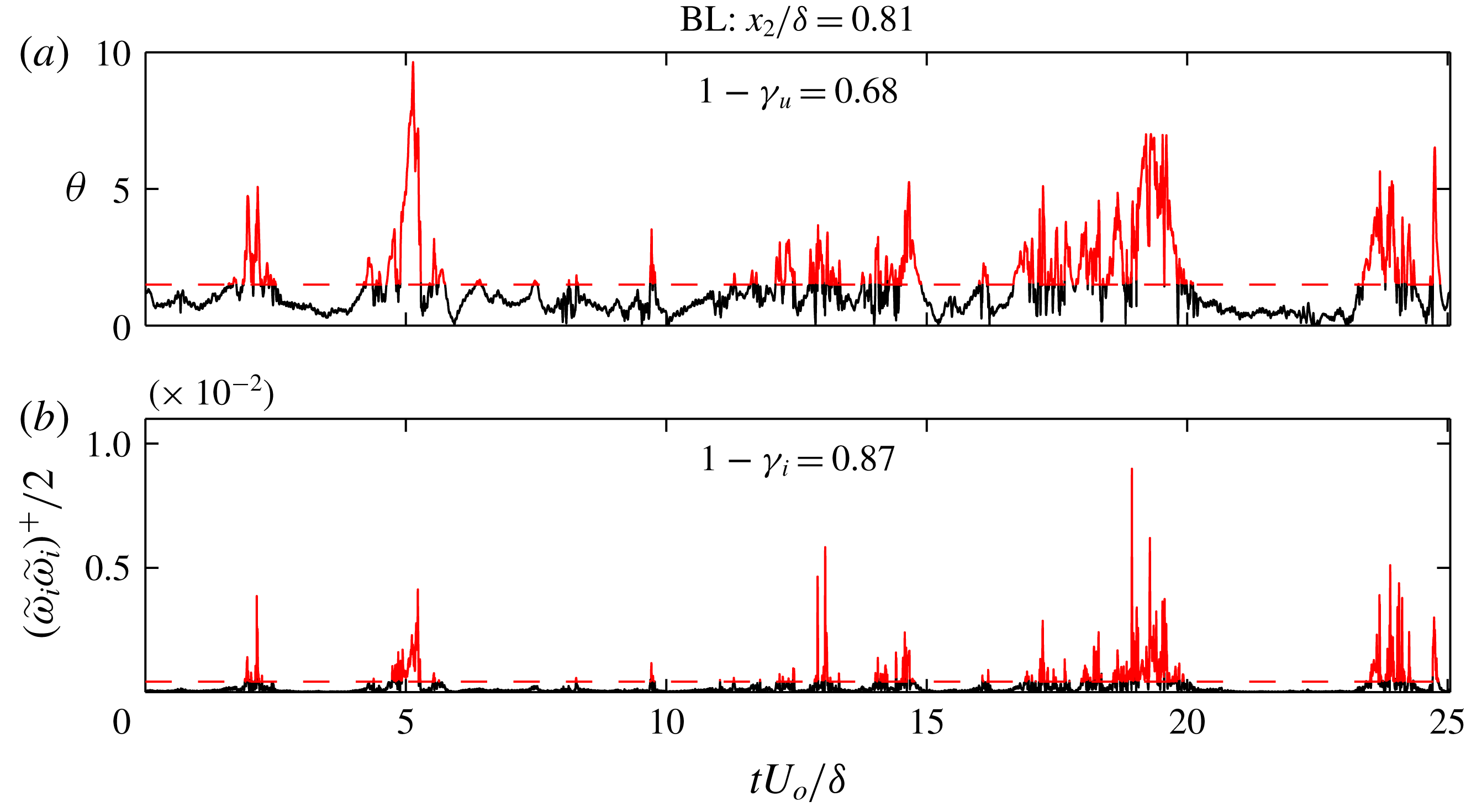
Figures 12(a) and 12(b) respectively show examples of the flow angle
 $\unicode[STIX]{x1D703}$
and the enstrophy time series that are used to evaluate irrotationality and unidirectionality. As both quantities are expected to be close to zero within a patch of ‘non-turbulent’ flow, it is expected that the two time series exhibit some degree of correspondence. Indeed, the correlation coefficient between the two is positive everywhere for both flows (
 ${\approx}0.1$
), and forms a peak in the ZPG wake (
 ${\approx}0.35$
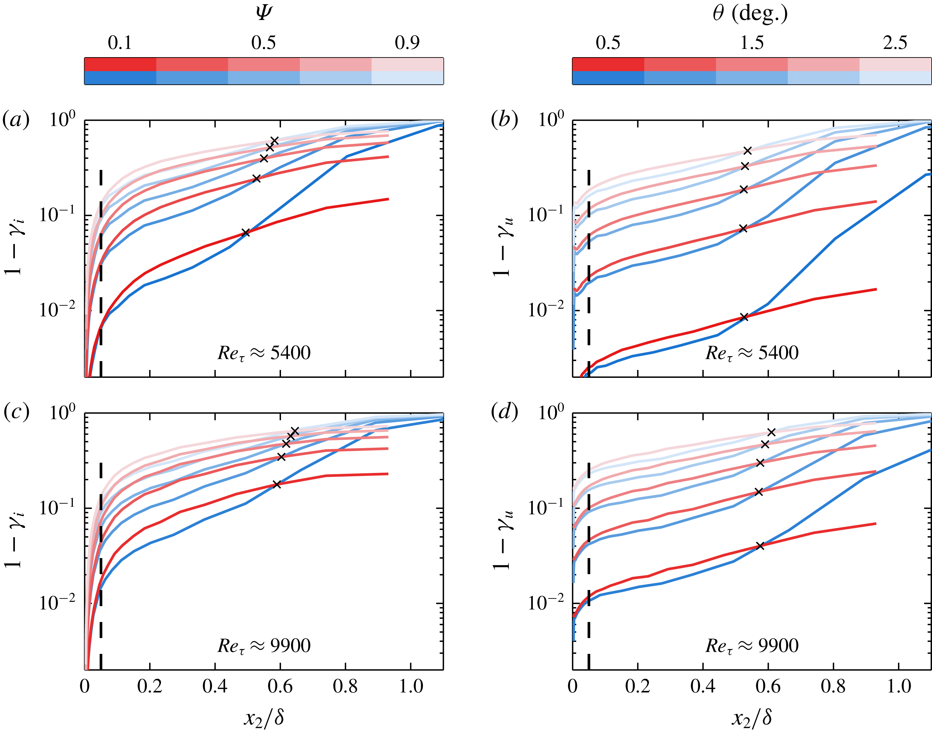
). The time fractions of signal that lie above the unidirectional and irrotational thresholds (shown in red) are denoted as
 $\unicode[STIX]{x1D6FE}_{u}$
and
 $\unicode[STIX]{x1D6FE}_{i}$
, respectively. These time fractions are computed for a range of thresholds at each wall-normal position, and are shown (as
 $1-\unicode[STIX]{x1D6FE}_{u}$
and
 $1-\unicode[STIX]{x1D6FE}_{i}$
) in figure 13. Note that darker shades in figure 13 correspond to lower thresholds.
Time series of flow angle
 $\unicode[STIX]{x1D703}$
and instantaneous enstrophy in the outer region of boundary layer flow at
 $Re_{\unicode[STIX]{x1D70F}}\approx 5600$
. Thresholds of
 $1.5^{\circ }$
and
 $5\times 10^{-4}$
for
 $\unicode[STIX]{x1D703}$
and enstrophy, respectively, are indicated by red dashed lines. Red-coloured time series segments exceed the plotted threshold.

(a,c) Fraction of time in which instantaneous enstrophy falls below a range of thresholds for pipe and boundary layer flow. (b,d) Fraction of time in which instantaneous flow angle relative to the
 $x_{1}$
direction (i.e.
 $\unicode[STIX]{x1D703}$
) falls below a range of thresholds for pipe and boundary layer flow. Here
 $\unicode[STIX]{x1D6FE}$
refers to the time fraction of the flow that is ‘turbulent’, and subscripts
 $i$
and
 $u$
here respectively refer to the irrotationality and unidirectionality criteria for determining turbulent/non-turbulent status. Red curves represent pipe flow, blue curves represent ZPG boundary layer flow. Black
 $\times$
symbols indicate cross-over points where time fractions for pipes and boundary layers are equal at each threshold. Black dashed lines at
 $x_{2}/\unicode[STIX]{x1D6FF}\approx 0.05$
are included for reference in each.

Figure 13 reveals several fundamental differences in the organization of pipe and boundary layer flows. From just interior to the outer boundary of the log layer to the middle of the wake (i.e.
 $x_{2}/\unicode[STIX]{x1D6FF}\approx 0.05$
–
 $0.5$
), the boundary layer can be characterized as more ‘well stirred’ than the pipe, as a smaller time fraction of boundary layer flow falls below each threshold for both the unidirectionality and irrotationality criteria. Magnitude differences between the two
 $Re_{\unicode[STIX]{x1D70F}}$
cases, particularly for the lowest thresholds, are most likely influenced by spatial resolution, and thus conclusions drawn from figure 13 should be limited to those based on the relative magnitudes of the pipe and boundary layer, and the dependence of these relative magnitudes on wall distance.
The location of the discrepancy between ‘non-turbulent’ time fractions in the two flows roughly corresponds to the outer ‘bump’ in the boundary layer enstrophy relative to pipe enstrophy, the largest differences in Reynolds stresses between the two flows and the lower magnitudes of boundary layer skewness and kurtosis profiles for a number of quantities as discussed throughout §§ 3 and 4. Beginning at
 $x_{2}/\unicode[STIX]{x1D6FF}\approx 0.5$
, the boundary layer sees a rapid rise in the portion of flow that can be characterized as ‘non-turbulent’. The location of this abrupt change is consistent with the onset of peaks in numerous third and fourth order boundary layer statistics, and thus supports the notion that these phenomena are related to the onset of ‘external’ intermittency. At
 $x_{2}/\unicode[STIX]{x1D6FF}\approx 0.55$
, the pipe and boundary layer have simultaneously equal fractions of both quasi-irrotational and quasi-unidirectional flow. Beyond this cross-over point, however, the boundary layer fully transitions to the free stream while the pipe maintains a finite level of enstrophy and turbulence intensity.
The statistics first shown in figure 11 are plotted again in figure 14 for the
 $Re_{\unicode[STIX]{x1D70F}}\approx 5400$
case, along with a family of curves showing the effect of removing ‘non-turbulent’ regions. Figure 14(b) reveals that the outer ‘bump’ in the ratio of boundary layer enstrophy to pipe enstrophy is diminished when quasi-irrotational flow is removed from consideration. When the threshold is taken as 90 % of the value at
 $x_{2}^{\ast }$
(i.e.
 $\unicode[STIX]{x1D6F9}=0.9$
), the ratio of boundary layer to pipe enstrophy is essentially flat. Furthermore, the enstrophy ratio is unchanged by the removal of quasi-irrotational signal at
 $x_{2}/\unicode[STIX]{x1D6FF}\approx 0.55$
, which corresponds to the intersections of
 $1-\unicode[STIX]{x1D6FE}_{i}$
for the two flows as shown in figure 13. Thus, the observed discrepancy in enstrophy profile shape in the wake region is due to the difference in the time fraction of each flow in which instantaneous enstrophy is very low. The highly super-Gaussian kurtosis of all three vorticity components suggests that the enstrophy signal is composed of ‘bursts’ having magnitudes that far exceed the signal root mean square. That the ratio shown in figure 14(b) becomes flat and close to unity by removing ‘non-turbulent’ regions suggests that the mean enstrophy of these ‘bursts’ is the same in pipe and boundary layer flows of the same
 $Re_{\unicode[STIX]{x1D70F}}$
at any wall distance.
Effect of removing ‘non-turbulent’ patches on quantities plotted in figure 11. (a) Mean enstrophy of ‘turbulent’ patches in pipe and boundary layer flow at
 $Re_{\unicode[STIX]{x1D70F}}\approx 5400$
. (b) Ratio of ‘turbulent’ patch mean enstrophy between boundary layer and pipe at
 $Re_{\unicode[STIX]{x1D70F}}\approx 5400$
.

6 Conclusions
A multi-sensor hot-wire probe capable of measuring both the velocity and vorticity vectors has been deployed in a set of three turbulent pipe flows and three zero pressure gradient boundary layers with nominally matched inner and outer scales. The present results represent the first physical measurements of kinetic energy and enstrophy in pipe and ZPG boundary layer flows with matched
 $Re_{\unicode[STIX]{x1D70F}}$
and spatial resolution conditions, as well as the highest
 $Re_{\unicode[STIX]{x1D70F}}$
simultaneous measurements of these quantities in pipe flow. Basic statistical results of these measurements are presented and highlight differences between the two flows and identify the subdomain over which they occur. A number of the observed differences in the present study match the observations of several lower-
 $Re_{\unicode[STIX]{x1D70F}}$
DNS and experimental studies, including those of Jiménez & Hoyas (Reference Jiménez and Hoyas2008), Monty et al. (Reference Monty, Hutchins, Ng, Marusic and Chong2009) and El Khoury et al. (Reference El Khoury, Schlatter, Noorani, Fischer, Brethouwer and Johansson2013).
Differences are observed in the
 $u_{2}$
and
 $u_{3}$
variance profiles from at least
 $x_{2}^{+}\approx 2.6\sqrt{\unicode[STIX]{x1D6FF}^{+}}$
, with the maximum difference occurring at
 $x_{2}/\unicode[STIX]{x1D6FF}\approx 0.3$
. The location of the maximum difference in
 $u_{2}$
and
 $u_{3}$
variance profiles is also characterized by smaller boundary layer skewness and kurtosis magnitudes (of both velocity and vorticity components), as well as higher boundary layer turbulence enstrophy (or to a close approximation, turbulence dissipation) relative to the pipe. It is then shown that the same region features a higher time fraction of pipe flow that can be characterized quasi-irrotational and quasi-unidirectional. Accounting for this difference largely eliminates the discrepancy in enstrophy between the two flows.
Aside from slight deviations near
 $x_{2}/\unicode[STIX]{x1D6FF}\approx 0.3$
as noted above, third- and fourth-order statistics of both velocity and vorticity components for the pipe cases closely match those of the ZPG boundary layer from the near wall until the emergence of intermittency-related outer magnitude peaks in the boundary layer profiles. With the exception of the outer peak in the boundary layer
 $u_{2}$
skewness, which emerges at
 $x_{2}/\unicode[STIX]{x1D6FF}\approx 0.35$
, these peaks generally emerge near
 $x_{2}/\unicode[STIX]{x1D6FF}\approx 0.5$
–0.6. The pipe and boundary layer velocity variances also intersect at approximately
 $x_{2}/\unicode[STIX]{x1D6FF}\approx 0.6$
, beyond which the boundary layer variances decay to zero while those in the pipe do not. The agreement in position between the point at which the velocity variances intersect and the point at which the higher-order statistics rapidly increase in magnitude supports the hypothesis of Schubauer (Reference Schubauer1954) – that the distribution of turbulent energy in a pipe is the same as in the ‘turbulent’ patches of a boundary layer in the region above
 $x_{2}/\unicode[STIX]{x1D6FF}\approx 0.6$
. Despite the absence of purely irrotational potential flow at the outer boundary, velocity fluctuations in the pipe also trend away from Gaussian behaviour in the wake. This is consistent with the existence of a ‘quiescent core’ in a pipe flow (Kwon et al. (Reference Kwon, Philip, de Silva, Hutchins and Monty2014) detected this feature in a channel flow) and the associated intermittency between high- and low-level turbulent regions.
Cross-stream velocity component fluctuations exhibit super-Gaussian kurtosis throughout the entire flow domain for both pipe and boundary layer flows, while streamwise velocity fluctuations remain sub-Gaussian until the wake. The kurtosis coefficients of the vorticity fluctuations of all three components are super-Gaussian across the flow domain, with the kurtosis of the zero-mean components (
 $\unicode[STIX]{x1D714}_{1}$
and
 $\unicode[STIX]{x1D714}_{2}$
) tending to increase with distance from the wall. The spanwise vorticity skewness is of the same sign as the mean vorticity across the flow domain, and trends toward zero at an approximately logarithmic rate in the region where the mean velocity is logarithmic.
Acknowledgements
This work was supported by the Australian Research Council and the National Science foundation under award number NSF-CBET 12447698. The authors would also like to extend their gratitude to the authors of Sillero et al. (Reference Sillero, Jiménez and Moser2013) for allowing access to their DNS volumes.
Appendix A. HRNBLWT measurements
Owing to the slight departures from the expected canonical ZPG wake behaviour of the Flow Physics Facility (FPF) measurements (cf. figure 3), additional measurements collected at the High Reynolds Number Boundary Layer Wind Tunnel (HRNBLWT) – and adhering more strictly to the canonical wake shape – are included in this appendix. These measurements are not included in the main text because they correspond to lower-
 $Re_{\unicode[STIX]{x1D70F}}$
cases (about
 $2/3$
the magnitude of those collected at the FPF and in the pipe flow, for matched spatial resolution), and to avoid overcrowding the figures. The parameters of these measurements are given in table 2. The parameters of the pipe measurements are also reproduced in table 2 (from table 1) for reference.
(a) Mean streamwise velocity in log-law form. Experimental profiles plotted as solid lines capped by symbols for clarity. Symbols at start/end of each line correspond to table 2. (b) Mean streamwise velocity in defect form. Symbols as in table 2, thick solid lines represent DNS (see table 1).

Summary of experiments presented in appendix A.

Figure 15 contains the same plots of mean velocity in log-law and deficit form as shown in figure 3, but with the HRNBLWT measurements in place of the FPF measurements. As can be seen from figure 15
 $(b)$
in particular, the HRNBLWT data closely match the DNS of Sillero et al. (Reference Sillero, Jiménez and Moser2013) through the log layer and wake. Thus, the wake region features seen in the HRNBLWT data in the following figures are not expected to feature any artefacts associated with departures from the canonical wake shape.
Figure 16 shows the profiles of Reynolds stress of the pipe and boundary layer cases as measured in the CICLoPE and the HRNBLWT, respectively, along with selected results from existing studies. The deviations in the
 $u_{2}$
and
 $u_{3}$
variance profiles are the same as those identified using the FPF data in § 3. The present
 $\overline{u_{2}}^{2}$
and
 $\overline{u_{3}}^{2}$
profiles exhibit very close agreement with those of Baidya (Reference Baidya2015), which were obtained via a
 $\times$
-wire hot-wire array. The present
 $\overline{u_{2}}^{2}$
profiles agree in trend with those of Morrill-Winter et al. (Reference Morrill-Winter, Klewicki, Baidya and Marusic2015), which were obtained with a specialized 4-wire hot-wire probe, though with a slight difference in magnitude. Such differences highlight the advantage of using the same measurement technique under matched conditions to compare pipe and boundary layer flow. Differences between the two flows in the wake portion of the Reynolds shear stress profiles are more clearly visible in figure 16(d) than in figure 7(a). Although no clear difference in the
 $u_{1}$
variance profile shapes could be identified from the comparison of the FPF and CICLoPE data, it could be argued that the HRNBLWT
 $u_{1}$
variance systematically exceeds that of the pipe over the region
 $0.3\lesssim x_{2}/\unicode[STIX]{x1D6FF}\lesssim 0.8$
when
 $\unicode[STIX]{x1D6FF}_{99}$
is used as the outer scale. This difference in
 $u_{1}$
variance in the outer region is highlighted in the inset to figure 16(a), which shows the two highest-
 $Re_{\unicode[STIX]{x1D70F}}$
cases along with highly resolved single-element hot-wire measurements for pipe flow at
 $Re_{\unicode[STIX]{x1D70F}}\approx 10\,500$
from Hultmark et al. (Reference Hultmark, Vallikivi, Bailey and Smits2013) and for boundary layer flow at
 $Re_{\unicode[STIX]{x1D70F}}\approx 8000$
from Samie et al. (Reference Samie, Marusic, Hutchins, Fu, Fan, Hultmark and Smits2018). When
 $\unicode[STIX]{x1D6FF}$
for the boundary layer is chosen as
 $\unicode[STIX]{x1D6FF}_{99}$
, this feature is reminiscent of the outer ‘bumps’ in the
 $u_{2}$
and
 $u_{3}$
variance profiles. While a slight change in the definition of
 $\unicode[STIX]{x1D6FF}$
for the boundary layer case could remove the difference between the two
 $u_{1}$
profiles in the outer region, it could not remove the observed differences in the
 $u_{2}$
or
 $u_{3}$
variance profiles.
(a–c) Streamwise, wall-normal, and spanwise Reynolds normal stress, and (d) Reynolds shear stress profiles as measured in the HRNBLWT and the CICLoPE. Shaded regions indicate range of inner log-layer boundaries for present experimental cases. ‘

 $Re_{\unicode[STIX]{x1D70F}}\approx 5200$
channel DNS from Lee & Moser (Reference Lee and Moser2015); ‘

 $Re_{\unicode[STIX]{x1D70F}}\approx 10\,500$
pipe data from Hultmark et al. (Reference Hultmark, Vallikivi, Bailey and Smits2013); ‘

 $Re_{\unicode[STIX]{x1D70F}}\approx 8000$
boundary layer data from Samie et al. (Reference Samie, Marusic, Hutchins, Fu, Fan, Hultmark and Smits2018); ‘

 $Re_{\unicode[STIX]{x1D70F}}\approx 8000$
boundary layer (HRNBLWT) data from Baidya (Reference Baidya2015);‘

 $Re_{\unicode[STIX]{x1D70F}}\approx 7900$
boundary layer (HRNBLWT) data from Morrill-Winter et al. (Reference Morrill-Winter, Klewicki, Baidya and Marusic2015). Log-line in (a) corresponds to
 $\overline{u_{1}^{2}}/U_{\unicode[STIX]{x1D70F}}^{2}=1.95-1.26\log (x_{2}/\unicode[STIX]{x1D6FF}_{99})+\log (1.15)$
from Marusic et al. (Reference Marusic, Monty, Hultmark and Smits2013), where the additional
 $\log (1.15)$
constant accounts for a difference in definition of
 $\unicode[STIX]{x1D6FF}$
. Log lines in (c) correspond to
 $\overline{u_{3}^{2}}/U_{\unicode[STIX]{x1D70F}}^{2}=1.66-0.26\log (x_{2}/\unicode[STIX]{x1D6FF}_{99})$
for the boundary layer and
 $\overline{u_{3}^{2}}/U_{\unicode[STIX]{x1D70F}}^{2}=1.11-0.42\log (x_{2}/\unicode[STIX]{x1D6FF})$
for the pipe. See tables 1 and 2 for remaining symbols/lines.

Figure 17 shows the skewness profiles of
 $u_{1}$
,
 $u_{2}$
and
 $u_{1}u_{2}$
as measured in the HRNBLWT and CICLoPE. These profiles clearly exhibit a trend of slightly lower boundary layer skewness magnitude from near the outer edge of the log layer out to
 $x_{2}/\unicode[STIX]{x1D6FF}\approx 0.5$
. These features are consistent with the differences in intermittency factor
 $\unicode[STIX]{x1D6FE}$
discussed in § 5. Quasi non-turbulent flow increases the probability density of fluctuating quantities close to 0, which in turn increases the magnitudes of skewness and kurtosis factors (if the fully turbulent portions of the flow remain relatively unchanged). Indeed, it was shown in § 5 that the time-fraction of quasi non-turbulent flow is higher in the pipe than the boundary layer from near the outer edge of the log-layer out to
 $x_{2}/\unicode[STIX]{x1D6FF}\approx 0.5$
.
(a,b) Skewness coefficient profiles for the fluctuating streamwise and wall-normal velocity signals, respectively, and (c) the fluctuating Reynolds shear stress signal. Symbols given in table 2.

(a–c) Kurtosis coefficient profiles respectively for the fluctuating streamwise, wall-normal, and spanwise velocity signals, and (d) the fluctuating Reynolds shear stress signal. Symbols given in table 2.

As with the skewness profiles shown in figure 17, the kurtosis profiles shown in figure 18 exhibit lower boundary layer profile magnitude near the outer edge of the log layer out to
 $x_{2}/\unicode[STIX]{x1D6FF}\approx 0.5$
. This feature is also clearly visible in the FPF
 $u_{3}$
kurtosis shown in figure 6(b), and to a lesser degree in the
 $u_{2}$
kurtosis shown in figure 5(c). Again, it is proposed that this feature is related to the difference in intermittency associated with the TNTI in the boundary layer and the quiescent core in the pipe.
Figure 19 contains the same plots of mean turbulence enstrophy and enstrophy ratio as figure 11, but with the HRNBLWT data plotted in place of the FPF data. The same outer ‘bump’ feature in the boundary layer enstrophy relative to the pipe enstrophy is visible in figure 19(b), but its onset (at
 $x_{2}/\unicode[STIX]{x1D6FF}\approx 0.1$
) is clearer and more consistent. Note that the ratio shown in figure 19(b) is multiplied by the ratio of Reynolds numbers
 $\unicode[STIX]{x1D6FF}_{BL}^{+}/\unicode[STIX]{x1D6FF}_{P}^{+}$
to account for the difference in enstrophy at a fixed
 $x_{2}/\unicode[STIX]{x1D6FF}$
location owing to the dependence of said enstrophy on (to an approximation)
 $x_{2}^{-1}$
.
(a) Inner-normalized turbulence enstrophy profiles plotted as sold lines capped by symbols for clarity. Symbols at start/end of each line correspond to table 2. (b) Ratio of turbulence enstrophy between boundary layers and pipes of approximately matched spatial resolution. Note the shorthand
 $\overline{\unicode[STIX]{x1D714}^{2}}=\overline{\unicode[STIX]{x1D714}_{i}\unicode[STIX]{x1D714}_{i}}$
is used in (b). Each ratio is multiplied by
 $\unicode[STIX]{x1D6FF}_{BL}^{+}/\unicode[STIX]{x1D6FF}_{P}^{+}$
to account for the apparent Reynolds number trend when ratios are computed based on
 $x_{2}/\unicode[STIX]{x1D6FF}$
coordinates (i.e. that associated with
 $\overline{\unicode[STIX]{x1D714}_{i}\unicode[STIX]{x1D714}_{i}}\sim x_{2}^{-1}$
dependence).

Appendix B. Vorticity resolution
The synthetic experimentally predicted effects of probe size on vorticity resolution are summarised in figure 20. Figure 20(a) shows the length of an individual wire relative to the local Kolmogorov length scale
 $\unicode[STIX]{x1D702}$
for the three spatial resolution cases corresponding to the present experimental data. Figure 20(b) shows the synthetic experimental predicted ratio of ‘measured’ (subscript
 $m$
) to ‘true’ (subscript
 $m$
) vorticity r.m.s. magnitude
 $|\unicode[STIX]{x1D714}|$
, defined as
 $$\begin{eqnarray}\displaystyle |\unicode[STIX]{x1D714}|=(\unicode[STIX]{x1D714}_{1}^{2}+\unicode[STIX]{x1D714}_{2}^{2}+\unicode[STIX]{x1D714}_{3}^{2})^{1/2}, & & \displaystyle\end{eqnarray}$$
a function of
 $l_{w}/\unicode[STIX]{x1D702}$
. The light and dark shaded regions in figure 20(a,b) correspond to the inner and outer boundaries of the log layer for the range of experimental data presented herein. Recall from figure 2 and table 1 that the sub-array separation distances are related to the wire length as
 $\unicode[STIX]{x0394}x_{2}=l_{w}/\sqrt{2}$
and
 $\unicode[STIX]{x0394}x_{2}=2.5l_{w}/\sqrt{2}$
. Figure 20(b) indicates that approximately 85 % of the vorticity is resolved at the inner edge of the log layer for the highest resolution cases, and about 73 % for the lowest resolution (highest-
 $Re_{\unicode[STIX]{x1D70F}}$
). These percentages increase to approximately 90 % and 85 % respectively for the highest and lowest resolution cases at the outer edge of the log layer. The focus of most of the conclusions surrounding vorticity in the present paper is on the region near the outer edge of the log layer out to the middle of the wake, where the vorticity resolution will improve even further. Furthermore, specific conclusions regarding the vorticity are limited herein only to comparisons of measurements at matched resolution.
(a) Synthetic experiment predicted magnitude of reference length
 $l_{w}$
relative to Kolmogorov length scale
 $\unicode[STIX]{x1D702}$
. Light and dark shaded regions respectively indicate the range of inner and outer boundaries of the log layer (
 $x_{2_{i}}$
and
 $x_{2_{o}}$
) for the physical experimental datasets presented herein. (b) Synthetic experiment ‘measured’ (subscript
 $m$
) versus ‘true’ (subscript
 $t$
) vorticity r.m.s. magnitude captured by the present probe geometry as a function of reference length
 $l_{w}$
relative to
 $\unicode[STIX]{x1D702}$
. Light and dark shaded regions respectively indicate range of probe resolutions at the start and end of the log layer for the physical experimental cases.

Given that the synthetic experiment corresponds to a lower Reynolds number (
 $Re_{\unicode[STIX]{x1D70F}}\approx 2000$
) than the present measurements, an additional comment on the effects of
 $Re_{\unicode[STIX]{x1D70F}}$
is warranted. As can be seen from figure 20(b), resolution of the vorticity signal is (to a close approximation) dependent on the local value of the Kolmogorov length scale
 $\unicode[STIX]{x1D702}$
relative to the size of the probe (e.g. see also Zhu & Antonia Reference Zhu and Antonia1995). To the degree that the dissipation rate scales with
 $U_{\unicode[STIX]{x1D70F}}$
and
 $l_{\unicode[STIX]{x1D708}}$
from the wall through the log-layer (which is quite well based on available DNS and
 $\unicode[STIX]{x2202}u_{1}/\unicode[STIX]{x2202}x_{1}$
-based experimental estimates),
 $\unicode[STIX]{x1D702}$
is (at least for the present purposes) independent of
 $Re_{\unicode[STIX]{x1D70F}}$
in the near-wall region and where the log layers of two disparate
 $Re_{\unicode[STIX]{x1D70F}}$
flows overlap. Thus, the synthetic experimental predictions of vorticity resolution should apply even to the higher-
 $Re_{\unicode[STIX]{x1D70F}}$
experiments out to a viscous wall distance that corresponds to
 $x_{2}/\unicode[STIX]{x1D6FF}_{DNS}\approx 0.15$
, i.e.
 $x_{2}^{+}\approx 300$
. Above this position, the
 $\unicode[STIX]{x1D702}\sim x_{2}^{1/4}$
trend can be used to predict the values of
 $l_{w}/\unicode[STIX]{x1D702}$
at higher Reynolds numbers. The resolved fraction of vorticity magnitude may then be estimated according to figure 20(b).