2. Problem formulation

Consider two horizontal plates with a gap between them filled with a fluid, as shown in figure 1. The upper plate is smooth, while the lower one has sinusoidal corrugations, resulting in the gap geometry of the form

(2.1a,b)\begin{equation}y_L^\ast ({x^\ast }) = \, - {h^\ast } + \, 0.5\, {A^\ast }\ \textrm{cos}({\alpha ^\ast }{x^\ast }),\quad y_U^\ast ({x^\ast }) = {h^\ast },\end{equation}

where the subscripts L and U refer to the lower and upper plates, respectively, ${A^\ast }$ is the (peak to bottom) amplitude of the groove, ${\alpha ^\ast }$ is its wavenumber and stars identify dimensional quantities. The gap extends to ${\pm} \infty $ in the x*-direction, its mean opening is $2{h^\ast }$ and it is periodic with wavelength ${\lambda ^\ast } = 2{\rm \pi} /{\alpha ^\ast }$. The gravitational acceleration ${g^\ast }$ is acting in the negative y*-direction. The fluid is assumed to have a thermal conductivity ${k^\ast }$, specific heat ${c^\ast }$, thermal diffusivity ${\kappa ^\ast } = {k^\ast }/{\rho ^\ast }{c^\ast }$, kinematic viscosity ${\nu ^\ast }$, dynamic viscosity ${\mu ^\ast }$, thermal expansion coefficient ${\varGamma ^\ast }$ and variations of its density ${\rho ^\ast }$ follow the Boussinesq approximation. Conditions required for the use of this approximation are discussed by Tritton (Reference Tritton1977). Results of experiments for thermal conditions similar to those used in this analysis (Inasawa et al. Reference Inasawa, Taneda and Floryan2019, Reference Inasawa, Hara and Floryan2021; Floryan & Inasawa Reference Floryan and Inasawa2021) demonstrate that the Boussinesq approximation captures well the fluid response. These experiments included qualitative (flow topology) and quantitative (velocity measurements) comparisons with the theoretical model.

Figure 1.

Schematic diagram of the flow system.

The upper plate is free to move within its plane, and the lower plate is stationary. The upper plate does not move in the case of an isothermal system, as no mechanism is available to generate a propulsive force. The introduction of patterned heating produces convection in the slot, and it is interesting to determine if this convection can force movement of the upper plate. We assume that the heating applied to the lower plate results in a simple sinusoidal temperature distribution while the upper plate is kept isothermal, i.e.

(2.2a,b)\begin{equation}T_L^\ast ({x^\ast }) = T_{mean,L}^\ast+ 0.5\, T_{per}^\ast \ \textrm{cos}({\alpha ^\ast }{x^\ast } + {\varOmega ^\ast }),\quad T_U^\ast ({x^\ast }) = T_U^\ast ,\end{equation}

where the subscripts ‘mean’ and ‘per’ refer to the mean and periodic parts, respectively, $T_{per}^\ast $ is the peak-to-peak amplitude of the periodic component and ${\varOmega ^\ast }$ denotes the phase shifts between the heating and groove patterns. We use $T_U^\ast $ for reference with all material properties and define the relative temperature ${\theta ^\ast }\, = \, {T^\ast }\, \unicode{x2013}\, T_U^\ast $ to get

(2.3a,b)\begin{equation}\theta _L^\ast (x) = \theta _{uni}^\ast+ 0.5\, \theta _{per}^\ast \ \textrm{cos}({\alpha ^\ast }{x^\ast } + {\varOmega ^\ast }),\quad \theta _U^\ast (x) = \, 0,\end{equation}

where $\theta _{uni}^\ast= T_{uni}^\ast= T_{mean,L}^\ast- T_U^\ast $, $\theta _{per}^\ast= T_{per}^\ast $. Finally, we use half of the mean gap height ${h^\ast }$ as the length scale and ${\kappa ^\ast }{\nu ^\ast }/({g^\ast }{\varGamma ^\ast }{h^{{\ast} 3}})$ as the temperature scale to find the dimensionless expressions for the geometry and temperatures of the form

(2.4a,b)\begin{gather}{y_L}(x) = \, - 1 + 0.5A\ \textrm{cos}(x),\quad {y_U}(x) = \, 1,\end{gather}

(2.5a,b)\begin{gather}{\theta _L}(x) = R{a_{uni}} + 0.5R{a_{per}}\ \textrm{cos}(\alpha x + \varOmega ),\quad {\theta _U}(x) = 0,\end{gather}

where $R{a_{uni}} = {g^\ast }{\varGamma ^\ast }{h^{{\ast} 3}}T_{uni}^\ast{/}({\kappa ^\ast }{\nu ^\ast })$ is the uniform Rayleigh number measuring the intensity of the uniform heating component and $R{a_{per}} = {g^\ast }{\varGamma ^\ast }{h^{{\ast} 3}}T_{per}^\ast{/}({\kappa ^\ast }{\nu ^\ast })$ is the periodic Rayleigh number measuring the intensity of the periodic heating component. Determination of whether the heating can create a movement of the upper plate requires a solution of the field equations of the form

(2.6a,b)\begin{gather}\frac{{\partial u}}{{\partial x}} + \frac{{\partial v}}{{\partial y}} = 0,\quad u\frac{{\partial u}}{{\partial x}} + v\frac{{\partial u}}{{\partial y}} =- \frac{{\partial p}}{{\partial x}} + {\nabla ^2}u,\end{gather}

(2.6c,d)\begin{gather}u\frac{{\partial v}}{{\partial x}} + v\frac{{\partial v}}{{\partial y}} =- \frac{{\partial p}}{{\partial y}} + {\nabla ^2}v + P{r^{ - 1}}\, \theta ,\quad u\frac{{\partial \theta }}{{\partial x}} + v\frac{{\partial \theta }}{{\partial y}} = P{r^{ - 1}}{\nabla ^2}\theta ,\end{gather}

where ($u$, $v$) are the velocity components in the (x, y) directions, respectively, scaled with $\, {U_v}^\ast= {\nu ^\ast }/{h^\ast }$ as the velocity scale, p stands for the pressure scaled with$\, {\rho ^\ast }U_\nu ^{{\ast} 2}$ as the pressure scale and $Pr = {\nu ^\ast }/{\kappa ^\ast }$ denotes the Prandtl number. These equations are subject to the following boundary conditions:

(2.7a–c)\begin{gather}y =- 1 + 0.5A\ \textrm{cos}(x){:}\ u = v = 0,\quad \theta = R{a_{uni}} + 0.5R{a_{per}}\ \textrm{cos}(\alpha x + \varOmega ),\end{gather}

(2.7d–g)\begin{gather}y = 1{:}\ {\left. {\frac{{\partial u}}{{\partial y}}} \right|_{mean}} = 0,\quad {u_{per}} = 0,\quad v = 0,\quad \theta = 0.\end{gather}

One must impose constraints in the form of

(2.8)\begin{equation}{\left. {\frac{{\partial p}}{{\partial x}}} \right|_{mean}} = 0\end{equation}

to prevent any external pressure gradient from affecting the fluid movement. If convection generates a mean shear stress at the upper plate, then this plate accelerates until it reaches velocity ${U_{top}}$, which eliminates this stress – all forces acting on the upper plate must balance out, so, since the only permitted force is due to shear, the mean shear must be zero. The periodic components of shear do not matter as they cancel out over one period. The velocity of the upper plate ${U_{top}}$ is not known a priori – it is determined from the known solution during the postprocessing.

Identification of the plate driving forces requires evaluation of the surface forces acting on the plates. The stress vector at the lower plate ${\boldsymbol{\sigma }_L}$ is expressed as

(2.9) \begin{equation}{\boldsymbol{\sigma }_L} = \, [\begin{array}{*{20}{@{}cc@{}}} {{\sigma _{x,L}}}&{{\sigma _{y,L\, }}} \end{array}] = [\begin{array}{*{20}{@{}cc@{}}} {{n_{x,L}}}&{{n_{y,L}}} \end{array}]\left[ {\begin{array}{*{20}{@{}cc@{}}} {2\dfrac{{\partial u}}{{\partial x}} - p}&{\dfrac{{\partial u}}{{\partial y}} + \dfrac{{\partial v}}{{\partial x}}}\\ {\dfrac{{\partial u}}{{\partial y}} + \dfrac{{\partial v}}{{\partial x}}}&{2\dfrac{{\partial v}}{{\partial y}} - p} \end{array}} \right]\! ,\end{equation}

where ${\boldsymbol{n}_L} = ({n_{x,L}},{n_{y,L}}) = {N_L}(\textrm{d}{y_L}/\textrm{d}x, - 1)$, ${N_L} = {[1 + {(\textrm{d}{y_L}/\textrm{d}x)^2}]^{ - 1/2}}$, is the normal unit vector pointing outwards. The x-component of this vector has the form

(2.10)\begin{equation}{\sigma _{x,L}} = {\sigma _{xv,L}} + {\sigma _{xp,L}} = {N_L}\left[ {2\frac{{\textrm{d}{y_L}}}{{\textrm{d}x}}\frac{{\partial u}}{{\partial x}} - \left( {\frac{{\partial u}}{{\partial y}} + \frac{{\partial v}}{{\partial x}}} \right)} \right] - {N_L}\frac{{\textrm{d}{y_L}}}{{\textrm{d}x}}p,\end{equation}

where $({\sigma _{xv,L}},{\sigma _{xp,L}})$ denote the viscous and pressure contributions, respectively. The x-component of the total force ${F_{x,L}}$ acting on the fluid at the lower plate per unit length has the form

(2.11)\begin{align}{F_{x,L}} = {F_{xv,L}} + {F_{xp,L}} = {\lambda ^{ - 1}}\int_0^\lambda {\left[ {2\frac{{\textrm{d}{y_L}}}{{\textrm{d}x}}\frac{{\partial u}}{{\partial x}} - \left( {\frac{{\partial u}}{{\partial y}} + \frac{{\partial v}}{{\partial x}}} \right)} \right]\textrm{d}x} - {\lambda ^{ - 1}}\int_0^\lambda {\frac{{\textrm{d}{y_L}}}{{\textrm{d}x}}p\ \textrm{d}x} = 0,\end{align}

where ${F_{xp,L}}$ and ${F_{xv,L}}$ stand for the pressure and viscous contributions, which must be equal and opposite. Similar expressions for the upper plate have the form

(2.12a,b)\begin{equation}{\sigma _{x,U}} = {\sigma _{xv,U}} = {\left. {\frac{{\textrm{d}u}}{{\textrm{d}y}}} \right|_{y = 1}},\quad {F_{x,U}} = {F_{xv,U}} = {\lambda ^{ - 1}}\int_0^\lambda {{{\left. {\frac{{\textrm{d}u}}{{\textrm{d}y}}} \right|}_{y = 1}}\textrm{d}x} = 0,\end{equation}

and the total force must be null.

System (2.6)–(2.8) must be solved numerically with sufficient accuracy to provide a data quality suitable for analysing the effects of geometric irregularities and heating and their interactions. Modelling the irregularities requires using techniques able to accurately handle many geometries with an acceptable cost. The spectrally accurate immersed boundary method accomplishes this, as it provides both the necessary geometric flexibility and accuracy and the ability to handle many geometries with a minimum labour cost.

We express the field equations in terms of the stream function defined in the usual manner, i.e. $u = \partial \psi /\partial y,\,v =- \partial \psi /\partial x$, and normalized with condition $\psi (\kern0.7pt {y_L}) = 0$. Further, we capture the x-dependences of this function, as well as temperature $\theta $, by expressing them as Fourier expansions based on the wavenumber α. Then we substitute these expansions into the field equations and separate the Fourier modes formulating nonlinear, ordinary differential equations for the modal functions. We express the modal functions using Chebyshev expansions and employ the Galerkin projection method to construct algebraic equations for the expansion coefficients. The irregular shape of the lower plate is accommodated using the spectrally accurate immersed boundary conditions concept (Szumbarski & Floryan Reference Szumbarski and Floryan1999; Husain & Floryan Reference Husain and Floryan2008, Reference Husain and Floryan2010; Husain et al. Reference Husain, Szumbarski and Floryan2009). The resulting constraints expressing the flow and boundary conditions along the lower corrugated plate and boundary conditions along the smooth upper plate are accommodated using the tau method. The nonlinear algebraic equations resulting from the discretization process are solved using a fixed-point iterative technique. The discretization process provided spectral accuracy with the absolute error controlled by the number of Chebyshev polynomials and Fourier modes used in the computations. We determined that using 15 Fourier modes and 50 Chebyshev polynomials provided a minimum of five digit accuracy for all quantities of interest. The reader can find algorithm details in Panday & Floryan (Reference Panday and Floryan2021).

The heating activates different physical mechanisms. We begin the discussion by presenting these mechanisms in detail and then discuss the propulsion generated by these effects.

3. Thermal drift effect

We begin the discussion with a description of the thermal drift effect. If the upper plate does not experience any external resistance, viscous shear associated with convective motion may accelerate this plate until it reaches a velocity ${U_{top}}$ – the mean shear becomes zero under this condition.

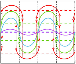
Typical velocity and temperature fields are illustrated in figure 2. When the hot spots are located at the groove crests $(\varOmega = 0)$, the flow topology is made of counter-rotating pairs of rolls with the fluid moving upwards above the hot spots (figure 2a). When the hot spots are located at the groove bottoms $(\varOmega = {\rm \pi})$, the flow field has a similar structure (figure 2c). All other positions of the hot spots result in the formation of a net horizontal flow directed either to the right $(0 < \varOmega < {\rm \pi})$ or to the left $({\rm \pi} < \varOmega < 2{\rm \pi} )$, as illustrated in figure 2(b,d), respectively. The flow direction is dictated by the relative position of the heating and groove patterns and represents a special form of thermal drift (Abtahi & Floryan Reference Abtahi and Floryan2017, Reference Abtahi and Floryan2018; Inasawa et al. Reference Inasawa, Hara and Floryan2021) driven by the pattern interaction effect (Floryan & Inasawa Reference Floryan and Inasawa2021).

Figure 2.

Flow and temperature fields for $\alpha = 2$, $A = 0.025$, $R{a_{uni}} = 0$, $R{a_{per}} = 500$ (a–d) corresponding to $\varOmega = 0,\,{\rm \pi} /2,\,{\rm \pi} ,\,3{\rm \pi} /2$, respectively. Dashed lines identify stream tubes carrying fluid in the horizontal direction.

The strength of the drift pulling the upper plate is quantified in terms of the velocity ${U_{top}}$. Typical variations of ${U_{top}}$ as a function of the phase shift $\varOmega $ illustrated in figure 3(a) demonstrate that positioning the hot spots either at $\varOmega = {\rm \pi}/2$ or at $\varOmega = 3{\rm \pi} /2$ produces the fastest plate movement. This speed increases proportionally to the groove amplitude, as illustrated in figure 3(b).

Figure 3.

Variation of the upper plate velocity ${U_{top}}$ (a) as a function of the phase shift $\varOmega$ and (b) as a function of the groove amplitude A for $\alpha = 2$, $Pr = 0.71$, $R{a_{per}} = 500$, $R{a_{uni}} = 0$. Thin dotted lines in (a) show $\varOmega $ giving rise to maximum ${U_{top}}$ and in (b) identify the character of the asymptotic variations for $A \to 0$.

Figure 4(a) illustrates the distribution of the x-component of the pressure force ${\sigma _{xp,L}}$ acting on the fluid at the lower plate that drives the fluid in the horizontal direction. The form of the pressure field is dictated by the convection pattern, whose structure, in turn, is dictated by the heating pattern. As this pattern moves relative to the grooves, the projection of the pressure field onto the surface topography changes, producing ${\sigma _{xp,L}}$ of different magnitudes and directions – this projection is responsible for horizontal fluid movement (Abtahi & Floryan Reference Abtahi and Floryan2017). The convective motion generates an x-component of the shear stress ${\sigma _{xv,L}}$ at the grooved plate with large periodic x-variations (see figure 4b). The mean value of the shear stress ${F_{xv,L}}/\lambda $ must be equal to the mean value of the pressure force ${F_{xp,L}}/\lambda $ as the upper plate does not support any forces.

Figure 4.

Distributions of (a) the x-component of the pressure force ${\sigma _{xp,L}}$ and (b) the x-component of the shear force ${\sigma _{xv,L}}$ acting on the fluid at the lower plate for $\alpha = 2$, $A = 0.025$, $R{a_{per}} = 500$, $R{a_{uni}} = 0$, $Pr = 0.71$ and $\varOmega = 0,\,{\rm \pi} /2,\,\, {\rm \pi},\,3{\rm \pi} /2$. The total forces are ${F_{xp,L}} = 0,\,1.49,\,0,\, - 1.49$, ${F_{xv,L}} = 0,\, - 1.49,\,0,\,1.49$ for $\varOmega = 0,\,{\rm \pi} /2,\,{\rm \pi} ,\,3{\rm \pi} /2$, respectively.

Uniform heating applied to the lower plate increases the plate velocity as the intensity of convection increases, while uniform cooling produces the opposite effect, as illustrated in figure 5(a). Reduction of the Prandtl number increases the strength of convection as mixing associated with convective motion is less effective in reducing horizontal temperature gradients (Hossain & Floryan Reference Hossain and Floryan2013, Reference Hossain and Floryan2022), leading to an increase of ${U_{top}}$, while its reduction has the opposite effect, as illustrated in figure 5(b).

Figure 5.

Variations of the upper plate velocity ${U_{top}}$ as a function of the phase shift $\varOmega $ for (a) $Pr = 0.71$, $R{a_{uni}} =- 100,\, - 50,\,0,\,50,\,100$, and for (b) $R{a_{uni}} = \, 0$, $Pr = 0.5,\,0.71$, 7. In both cases, $\alpha = 2$, $A = 0.05$ and $R{a_p} = 500$. Thick dashed lines in (a) show variations of the maximum of $|{{U_{top}}} |$ as a function of $\varOmega $. Term ‘multiplied by 5’ means that the quantity of interest was multiplied by a factor of 5 before plotting.

The stability of thermal drifts was assessed using the technique outlined in Appendix A. No unstable eigenvalues have been found, which suggests that thermal drifts are stable in the range of parameters of interest in this analysis.

4. Nonlinear thermal streaming effect

If the upper plate does not experience external resistance and the lower plate is smooth, sufficiently intense periodic heating may generate plate movement through nonlinear thermal streaming (Floryan Reference Floryan2023). The fluid motion has the form of counter-rotating rolls, as illustrated in figure 6. These rolls generate viscous stresses at the upper plate. If plumes of heated fluid flow straight upwards, the flow exhibits left/right symmetry, and the resulting stress has no mean component. A sufficiently strong plume may tilt either to the left or right, producing a non-zero mean stress, which results in movement of the upper plate – the plate accelerates until the mean shear is eliminated.

Figure 6.

Flow and temperature fields for $\alpha = 2.1$, $A = 0$, $R{a_{uni}} = 0$ and $R{a_{per}} = (a)\,884,\,(b)\,1000, (c)\,1000,\,(d)\,1000$. Dashed lines identify stream tubes carrying fluid in the horizontal direction.

The plate movement results from a system bifurcation, as illustrated in figure 7. The heating intensity, as measured by $R{a_{per,cr}}$, must reach a minimum level that strongly depends on the heating wavenumber – the minimum corresponds to $R{a_{per,cr}} \approx 900$, it occurs at $\alpha \approx 2.1,$ rapidly increasing when the heating wavelength is too short or too long (see figure 7). The value of $R{a_{per,cr}}$ rapidly increases when the Prandtl number increases as convection reduces the horizontal temperature gradients required to initiate this effect (see figure 7b). An addition of uniform heating minimizes the intensity of periodic heating required to produce bifurcation. In contrast, constant cooling has the opposite effect (see figure 7c).

Figure 7.

Variations of the upper plate velocity ${U_{top}}$ (a) as a function of $R{a_{per}}$ for $R{a_{uni}} = 0$, $Pr = 0.71$, $\alpha = 1.1,\,2.1,\,2.7$, (b) as a function of $R{a_{per}}$ for $R{a_{uni}} = 0$, $\alpha = 2.1$, $Pr = 0.15,\,0.71,\,1$, 1.5 and (c) as a function of $R{a_{per}}$ for $\alpha = 2.1$, $Pr = \, 0.71$, $R{a_{uni}} = 100,\,50,\,0,\, - 50,\, - 100$. Groove amplitude $A = 0$ in all cases. The critical conditions for $\alpha = 1.1,\,2.1,\,2.7$ in (a) are $R{a_{per,cr}} = 1206,\,891.25,\,1091.25$, respectively. The critical conditions for $Pr = 0.15,\,0.71,\,1,\,1.5$ in (b) are $R{a_{per,cr}} = 228.5,\,891.25,\,1203.33,\,1730$, respectively. The critical conditions for $R{a_{uni}} = 100,\,50,\,0,\, - 50,\, - 100$ in (c) are $R{a_{per,cr}} = 605.83,\,747.5,\,891.25,\,1038.33,\,1185$, respectively. All critical conditions were determined using stability analysis.

5. Combined effect

When the thermal drift and streaming effects are active, the combined effect occurs for a sufficiently high heating intensity. One can estimate the minimum heating required to activate the streaming for the grooved plate by placing hot spots either at the groove peaks or at the groove troughs, as this eliminates thermal drift. Results in figure 8 demonstrate relatively minor changes in critical conditions to those found in the case of a smooth plate. The same results also illustrate different responses when the hot spots are placed at the groove troughs and the groove peaks.

Figure 8.

Variations of the upper plate velocity ${U_{top}}$ as a function of the heating intensity $R{a_{per}}$ for $\varOmega = 0,\,{\rm \pi} /2,\,{\rm \pi} ,\,3{\rm \pi} /2$, $A = 0.025$, $Pr = 0.71$, $R{a_{uni}} = 0$, $\alpha = 2$. Dotted lines provide the plate velocity achieved with smooth plates. The critical conditions are $R{a_{per,cr}} = 914,\,857.5$ for $\varOmega = 0,\, {\rm \pi}$ for a grooved plate, respectively, and $R{a_{per,cr}} = 884.5$ for the smooth plate. These conditions were determined using stability theory.

The combined system response depends on the relative position of the heating and groove patterns, as illustrated in figure 9(a). The value of ${U_{top}}$ varies as a function of phase difference $\varOmega $ in a regular, nearly sinusoidal manner for $R{a_{per}} = 500$, which means that the flow response is driven by thermal drift and nonlinear streaming plays no role. Increase heating intensity to $R{a_{per}} = 800$, i.e. an increase of a factor of 1.6, results in a rise in the maximum possible ${U_{top}}$ by a factor of 4.7 while retaining its sinusoidal variations with $\varOmega $. When heating intensity is further increased to $R{a_{per}} = 900$, variations of ${U_{top}}$ remain regular, except when the phase difference is near $\varOmega = {\rm \pi}$, which corresponds to hot spots near the groove troughs. Nonlinear streaming becomes activated, leading to the appearance of limit points in variations of ${U_{top}}$ as a function of $\varOmega $ – for such conditions, a slight change of $\varOmega $ can change the direction of plate movement. System response shows hysteresis – when $\varOmega $ increases towards $\varOmega = {\rm \pi}$ and crosses the value of 3.23, ${U_{top}}$ jumps from ${U_{top}} = 1.53$ to ${U_{top}} =- 2.46$. When $\varOmega $ decreases back, ${U_{top}}$ does not jump back until the phase shift reaches a value of $\varOmega = 3.06$, when it jumps from ${U_{top}} =- 1.67$ to ${U_{top}} = 2.43$. The hysteresis loop is relatively narrow, i.e. it occurs between $\varOmega = 3.06$ and $\varOmega = 3.23$, with ${U_{top}}$ being positive at the upper side of the loop and negative at the lower side. Increasing the heating intensity to $R{a_{per}} = 1000$ results in the formation of additional limit points near $\varOmega = 0$, which correspond to hot spots near the groove peaks with another hysteresis loop forming there and a widening of the hysteresis loop near $\varOmega = {\rm \pi}$. Stability analysis (see Appendix A for details) demonstrates that the formation of limit points corresponds to the loss of stability of a particular branch of the bifurcation diagram (figure 9b). No stationary unstable states were found past the limit points, which suggests that only non-stationary states may exist under such conditions.

Figure 9.

(a) Variations of the upper plate velocity ${U_{top}}$ as a function of the phase shift $\varOmega $ for $\alpha = 2$, $A = 0.025$, $Pr = 0.71$, $R{a_{uni}} = 0$ and $R{a_{per}} = 500,\,800,\,900,\,1000$. Circles identify limit points. The dotted lines provide the plate velocity achieved with smooth plates. (b) Variations of the disturbance amplification rate ${\sigma _i}$ (see Appendix A for definition) as a function of the phase shift $\varOmega $ for flow conditions corresponding to red lines in (a). These disturbances are characterized by frequency ${\sigma _r} = 0$ (see Appendix A for definition).

Evolution of ${U_{top}}$ as a function of $R{a_{per}}$ near $\varOmega = 0$, which corresponds to hot spots near the groove peaks, is illustrated in figure 10(a). Using $\varOmega = 0$ results in a symmetric pitchfork bifurcation, i.e. the upper plate moves either to the right or to the left in the same manner. Placement of the hot spot very close to the groove peak and on its left side $(\varOmega = 0.08)$ produces plate movement to the right, with ${U_{top}}$ increasing monotonically with $R{a_{per}}$, i.e. no bifurcation takes place. A separate solution branch corresponding to the plate moving to the left appears when $R{a_{per}} > \, 850$. This branch does not connect to the branch describing plate movement to the right – it ends at a limit point at $R{a_{per}} = 956$ with ${U_{top}} =- 1.49$. Moving the hot spot further away to the left $(\varOmega = 0.52)$ produces a similar response but with ${U_{top}}$ varying with $R{a_{per}}$ in a more regular manner and with a new solution branch forming at a larger $R{a_{per}}$, i.e. the limit point of the new branch is at $R{a_{per}} = 1056$ with ${U_{top}} =- 2.71$. Placing a hot spot on the right side of the groove peak $(\varOmega =- 0.08)$ forces plate movement to the right with a new solution branch corresponding to negative ${U_{top}}$ appearing at a limit point $R{a_{per}} = 956$ and ${U_{top}} = 1.49$. Moving the hot spot further away $(\varOmega =- 0.52)$ moves the limit point to $R{a_{per}} = 956$ and ${U_{top}} =- 1.49$.

Figure 10.

Variations of the upper plate velocity ${U_{top}}$ as a function of the heating intensity $R{a_{per}}$ for (a) $\varOmega $ near 0, i.e. $\varOmega =- 0.52,\, - 0.08,\,0,\,0.08,\,0.52$, and (b) $\varOmega $ near ${\rm \pi} $, i.e. $\varOmega = {\rm \pi}- 0.52,\,{\rm \pi} - 0.08,\,{\rm \pi} + 0.08,\,{\rm \pi} + 0.52$. All results are for $A = 0.025$, $\alpha = 2$, $Pr = 0.71$, $R{a_{uni}} = 0$. Circles identify limit points. The dotted lines provide the plate velocity achieved with smooth plates. The critical conditions determined using stability theory are $R{a_{per,cr}} = 910,\,855$ for $\varOmega = 0,\, {\rm \pi}$ for a grooved plate, respectively, and $R{a_{per,cr}} = 880$ for the smooth plate. Dashed lines provide data for $\varOmega = {\rm \pi}$ (red) and $\varOmega = 3{\rm \pi} /2$ (blue).

Variations of ${U_{top}}$ as a function of $R{a_{per}}$ near $\varOmega = {\rm \pi}$, which correspond to hot spots located near the groove troughs, are qualitatively similar to those observed for $\varOmega $ near 0 (see figure 10b). Using $\varOmega = {\rm \pi}$ leads to a symmetric pitchfork bifurcation. Moving the hot spot to the left of the trough $(\varOmega = 0.08)$ produces negative ${U_{top}}$, which is a monotonic function of $R{a_{per}}$. A second branch, corresponding to positive ${U_{top}}$, appears at $R{a_{per}} = 896$ with ${U_{top}} = 1.39$. Moving the hot spots further away to the left $(\varOmega = 0.52)$ produces more regular variations of ${U_{top}}$ as a function of $R{a_{per}}$, with the second branch originating at $R{a_{per}} = 1000$ with ${U_{top}} = 2.7$. Moving the hot spot to the right produces a near mirror image of flow response with limit points being at $R{a_{per}} = 896$ and ${U_{top}} =- 1.39$ for $\varOmega =- 0.08$ and $R{a_{per}} = 1000$ and ${U_{top}} =- 2.7$ for $\varOmega =- 0.52$.

Comparisons of the data displayed in figures 8–10 show regular variations of ${U_{top}}$ as a function of $R{a_{per}}$ for $R{a_{per}} < \sim 800$, where thermal drift dominates, and regular variations for $R{a_{per}} > \sim 1100$ where, depending on $\varOmega $, either nonlinear streaming or thermal drift dominates, producing a nearly identical system response. The system response exhibits somewhat unpredictable but significant changes of ${U_{top}}$, including changes of direction for $R{a_{per}}$ varying between these limits.

The effectiveness of thermal drift increases proportionally to the groove amplitude, as illustrated in figure 3(b). When thermal streaming is active, variations of ${U_{top}}$ with A become complex and change with $\varOmega $ and $R{a_{per}}$ as illustrated in figure 11. Figure 11(a) shows the system response for $R{a_{per}} = \, 900$, which is just above the critical heating of $R{a_{per}} = \, 880$ for a smooth plate. No bifurcation occurs at $A = 0.0004$, but one occurs at $A = \, 0.0006$, producing wide hysteresis loops. Further increase of the amplitude to $A = 0.005$ dramatically narrows down the hysteresis loop. Further increase to $A = 0.02$ appears to change the magnitude of ${U_{top}}$ but does not affect the size of the hysteresis loop. Figure 11(b) illustrates what happens when heating corresponds to $R{a_{per}} = \, 1000$. No bifurcation occurs for $A = \, 0.005$ and $A = \, 0.0093$, but one is formed when the amplitude reaches $A = \, 0.0094$. The results show that the amplitude must increase by a factor of nearly 10 to produce bifurcation when heating increases from $R{a_{per}} = \, 900$ to $R{a_{per}} = \, 1000$. The hysteresis loop is very narrow at $A = \, 0.0094$ but significantly widens when the amplitude increases to $A = 0.025,$ which demonstrates a trend opposite to that observed for $R{a_{per}} = \, 900$.

Figure 11.

Variations of the upper plate velocity ${U_{top}}$ as a function of the phase shift $\varOmega $ for (a) $R{a_{per}} = \, 900$, $A = 0,\,0.001,\,0.005,\,0.02$, and (b) for $R{a_{per}} = \, 1000$, $A = 0,\,0.005,\,0.0093,\,0.0094,\,0.025$. All results are for $= 2$, $R{a_{uni}} = 0$ and $Pr = 0.71$. Circles identify limit points. Black dashed lines provide the plate velocity achieved with smooth plates. Positions of limit points were determined using stability theory.

Uniform heating strengthens thermal drift (see figure 5a) and reduces the critical Rayleigh number required for the onset of thermal streaming (see figure 7c). Effects of adding uniform heating when both effects are active are illustrated in figure 12. In general, uniform cooling reduces ${U_{top}}$ and eliminates bifurcations that would occur with uniform cooling. Heating has the opposite effect, as it lowers the critical Rayleigh number and increases the achievable ${U_{top}}$.

Figure 12.

Variations of the upper plate velocity ${U_{top}}$ as a function of the phase shift $\varOmega $ for $\alpha = 2$, $A = 0.025$, $R{a_{per}} = 1000$, $Pr = 0.71$ and $R{a_{uni}} =- 100,\, - 50,\,0,\,50,\,100$. Circles identify limit points. Dashed lines provide the plate velocity achieved with smooth plates. Positions of limit points were determined using stability theory.

The type of fluid strongly affects the magnitude of ${U_{top}}$. The propulsive effect relies on horizontal temperature gradients, which diminish with an increase of $Pr$ as this leads to more intense convection resulting in a reduction of these gradients. The thermal streaming and drift are affected similarly, as illustrated in figures 5(b) and 7(b). The cumulative effect is shown in figure 13. Reduction of $Pr$ reduces the critical Rayleigh number and increases the magnitude of ${U_{top}}$. A slight increase of Prandtl number from $Pr = 0.71$ to $Pr = 1$ eliminates bifurcations and leads to a significant reduction of ${U_{top}}$.

Figure 13.

Variations of the upper plate velocity ${U_{top}}$ as a function of the phase shift $\varOmega $ for $\alpha = 2$, $A = 0.025$, $R{a_{uni}} = 0$. Here, $R{a_{per}} = 1000$ for $Pr = 0.55,\,0.71,\,1,\,1.5$. Circles identify limit points. Dashed lines provide the plate velocity achieved with smooth plates. Positions of limit points were determined using stability theory.

Stability analysis was carried out using the formulation described in Appendix A. No unstable eigenvalues have been found, which suggests that the flows generated by the combined thermal streaming and thermal drift reported here are stable.

6. Summary

Analysis of the propulsive effect generated by heated grooves has been carried out. The model problem consists of parallel horizontal plates with the upper plate free to move and the lower plate equipped with grooves and subject to periodic heating. Perfectly tuned sinusoidal groove and heating patterns were considered, i.e. the same wavenumber described them. Heating forced movement of the upper plate whose velocity was used to measure propulsion effectiveness.

Two effects contribute to propulsion. The first effect is produced by an interaction of groove and heating patterns creating a thermal drift representing a forced system response. The strength of this effect depends on the relative position of both patterns. The upper plate movement reaches the maximum when hot spots are located approximately half-way between the groove peaks and troughs. It changes direction depending if the hot spot is on the right or left side of the groove peak. Thermal drift disappears when the hot spots are located at the groove peaks or the groove troughs.

The second effect relies on nonlinear thermal streaming and requires sufficiently intense heating for its activation. This effect represents system bifurcation. Both the thermal drift and the nonlinear streaming are active simultaneously and generate plate movement regardless of the relative position of both patterns. Similar to pure thermal drift, the fastest plate movement occurs for hot spots half-way between the groove peaks and troughs. A somewhat slower movement results when hot spots are located near the groove peaks and troughs. Under such conditions, the direction and velocity of plate movement may change drastically in response to a slight change in the relative position of both patterns. The formation of limit points and hysteresis loops was observed in response to changes in the relative position of both patterns.

The magnitude of propulsion increases with a decrease in the Prandtl number and expands with the addition of a uniform heating component. Despite extensive testing, investigating the stability of flows generated by the heating failed to identify any unstable eigenvalue.