



1. Introduction
Shear-thinning gels have emerged as an important class of complex fluids relevant across diverse applications such as aerospace propulsion, pharmaceutical engineering, fire suppression, paint coating, ink-jet printing, agriculture and environmental transport processes. Their ubiquity arises from their highly tuneable rheological characteristics, specifically shear-thinning nature, viscoelasticity and yield-stress behaviour, which allow gels to perform certain functions that are not always possible with conventional Newtonian liquids.
In pharmaceutical and biomedical sectors, their applications are a crucial role in innovative drug-delivery routes, including transdermal, intranasal, injectable and mucosal delivery (Hoffman Reference Hoffman2012; Seliktar Reference Seliktar2012). Such gels also mimic biological fluids and tissues, making them essential for therapeutics owing to their biocompatibility and biodegradability (Santhosh & Genova Reference Santhosh and Genova2022; Barroca-Ferreira et al. Reference Barroca-Ferreira, Gomes, Sousa, Passarinha and Costa2024; Kaur et al. Reference Kaur, Gogoi, Sharma, Das, Azad, Pramanik and Pramanik2024; Wu et al. Reference Wu, Chen, Zhao, Li, Song, Xiong, Yang, Zhu and Hu2024). Airborne disease transmission through coughing, sneezing or speech involve mucosalivary fluids. They exhibit pronounced shear thinning and viscoelasticity that strongly influence the aerosol formation (Xie et al. Reference Xie, Li, Sun and Liu2009; Pairetti et al. Reference Pairetti, Villiers and Zaleski2021; Kant et al. Reference Kant, Pairetti, Saade, Popinet, Zaleski and Lohse2023; Li et al. Reference Li, Saade, Zaleski, Sen, Kant and Lohse2025). Moreover, gel-based alternatives are being explored for targeted deposition, drift reduction, controlled dispersion and efficient spraying of pesticides (Tadros Reference Tadros1990; Zhang & Liu Reference Zhang and Liu2011). In natural events such as sea-aerosol formation, underwater volcanic eruptions in the ocean have the potential to alter the climatical conditions (Perfit et al. Reference Perfit, Cann, Fornari, Engels, Smith, Ian Ridley and Edwards2003). The transport mechanism of convection of biopolymer-laden marine gels, lava and dust particles to the atmosphere is directly associated through ocean winds (Veron Reference Veron2015; Deike et al. Reference Deike, Lenain and Melville2017; Deike Reference Deike2022; Legendre Reference Legendre2024). These examples highlight the importance of understanding the behaviour of shear-thinning materials across both engineering and natural systems.
In the field of aerospace propulsion, gel fuels have gained increasing attention in recent years as a promising candidate between solid and liquid propellants (Rahimi et al. Reference Rahimi, Peretz and Natan2010; Padwal et al. Reference Padwal, Natan and Mishra2021). These fuels can be engineered to accommodate energetic metal particles owing to increased yield stress and viscosity, and they offer enhanced safety such as reduced volatility, improved storability and throttleability of fuel as per the requirements (Natan & Rahimi Reference Natan and Rahimi2002; Baek et al. Reference Baek, Kim, Han and Kim2011; Madhumitha & Karmakar Reference Madhumitha and Karmakar2024). However, the efficiency of such a system based on gel fuels primarily depends upon the atomization characteristics of gels. The process of atomization terminates with secondary breakup, which primarily involves aerodynamic fragmentation of ligaments or drops into finer child droplets. The final droplet statistics in every atomization technique is critically governed by the fundamental process of secondary atomization. Hence, this process of drop fragmentation has been studied extensively in the past in the case of Newtonian liquids (Jackiw & Ashgriz Reference Jackiw and Ashgriz2021, Reference Jackiw and Ashgriz2022; Joshi & Anand Reference Joshi and Anand2022; Ade et al. Reference Ade, Chandrala and Sahu2023; Kulkarni et al. Reference Kulkarni, Shirdade, Rodrigues, Radhakrishna and Sojka2023; Ade et al. Reference Ade, Kirar, Chandrala and Sahu2024; Niranjan et al. Reference Niranjan, Bodi and Gadgil2024). Recent studies have increasingly examined the aerodynamic breakup of a range of complex fluids. Chandra et al. (Reference Chandra, Sharma, Basu and Kumar2024) have found that elastic polymeric droplets exhibit early deformation similar to Newtonian liquids, but increase in elasticity delays the fragmentation process significantly. In the case of drops of molten metal, for instance, drops of galinstan and tin also deform like Newtonian liquids in the initial stages, but the formation of an oxide layer is shown to inhibit the bag growth, alter the rupture dynamics and produce coarse, irregular fragments unlike that of conventional bag breakup (Hopfes et al. Reference Hopfes, Petersen, Wang, Giglmaier and Adams2021; Joshi & Anand Reference Joshi and Anand2022; Winter et al. Reference Winter, Hopfes, Giglmaier and Adams2025). There are also attempts to study the secondary atomization of liquids of a wide variety of rheological characters. These include specific polymer-based systems, such as xanthan gum, guar gum and carboxymethyl cellulose, water–coal slurries and particulate suspensions (Antonov et al. Reference Antonov, Kuznetsov and Strizhak2021; Qian et al. Reference Qian, Zhong, Zhu and Lin2021; Wang et al. Reference Wang, Yao, Zhao, Shi and Liu2023; Xu et al. Reference Xu, Wang and Che2023, Reference Xu, Liu, Zhang, Wang and Che2024). In the aerobreakup of suspensions, multicomponent droplets highlighted that a droplet breaks up early in bag breakup mode as compared with its base liquid. Such a observation has been attributed to the particulate inhomogeneity in the suspension (Xu et al. Reference Xu, Wang and Che2023, Reference Xu, Liu, Zhang, Wang and Che2024). These studies indicate that the droplet breakup phenomenon in complex liquids differs from the conventional Newtonian liquids and the observed distinct features are specific to the type of the liquid, its homogeneity at microlevel and its rheology.
Recently, Jackiw & Ashgriz (Reference Jackiw and Ashgriz2021, Reference Jackiw and Ashgriz2022) provided a comprehensive theoretical model augmented with experimental findings for droplet breakup of low-viscosity Newtonian liquids. A detailed investigation by Niranjan et al. (Reference Niranjan, Bodi and Gadgil2024) on the applicability of this model for viscous liquid droplets showed that key model parameters are inherently dependent on the liquid’s physical properties, particularly viscosity. Niranjan et al. (Reference Niranjan, Bodi and Gadgil2024) also redefined the time scales in the model by considering the motion of a droplet through the jet shear layer. It is hence envisaged that through the rheological parameters, the nature of the complexity of the liquid may affect the breakup dynamics as it has been observed in other atomization problems (Keshavarz et al. Reference Keshavarz, Houze, Moore, Koerner and McKinley2016, Reference Keshavarz, Houze, Moore, Koerner and McKinley2020; Chandra et al. Reference Chandra, Sharma, Basu and Kumar2024; Ratnu & Gadgil Reference Ratnu and Gadgil2025). The extent to which this modelling framework can be generalized to non-Newtonian liquids with complex rheology remains uncertain and needs a systematic evaluation.
In the present experimental study, we aim to address and explore the unanswered questions related to the droplet fragmentation of shear-thinning gels. Carbopol-based hydrogels of varying shear-thinning nature are employed in the present work. The droplet breakup phenomenon is captured using high-speed imaging and the distinctive qualitative and quantitative features are compared with the equivalent Newtonian liquids. The next section provides details of the experimental methods and rheological characterization of gels. Section 3 discusses the quantitative measurements of droplet morphology, the phenomenology of breakup and child droplet statistics followed by conclusions.
2. Methods and materials
2.1. Experimental set-up
(a) Schematic representation of the experimental facility; (b) detailed nozzle geometry used in the present study; (c) velocity profiles for a few operating conditions at the droplet falling location at
 $S_x = 10$
mm downstream of the nozzle exit plane.

Figure 1. Long description
Panel A: A schematic diagram of the experimental facility. High-pressure air is directed into an air nozzle with a diameter of 30 millimeters. The setup includes a syringe pump, a camera for side view arrangements at different angles (far view, near view, and 45-degree view), a light source, a diffuser screen, a hub, and a trigger box. The flow direction is indicated, and the spatial orientation is marked with x, y, and z axes. Panel B: A detailed diagram of the nozzle geometry used in the study. Pressurized air enters through a 23-millimeter diameter inlet and passes through a honeycomb and mesh section before exiting the nozzle. The dimensions of various parts of the nozzle are labeled, including lengths and diameters. Panel C: A graph showing velocity profiles for different operating conditions at the droplet falling location 153 millimeters downstream of the nozzle exit plane. The y-axis represents the vertical position in millimeters, and the x-axis represents the jet velocity in meters per second. Different symbols and colors represent various velocities, and the positions of the nozzle upper and lower edges are marked.
The schematic of the experimental test facility is presented in figure 1(a), where a continuous air jet method is used to investigate the secondary breakup of shear-thinning hydrogels. The set-up consists of several key components: (i) a pressurized air storage tank maintained at 10 bar; (ii) a convergent nozzle with a diameter (
 $D$
) of 30 mm; (iii) a syringe pump (Unigenetics Instruments Pvt. Ltd.) with a G22 needle (outer diameter = 0.716 mm); (iv) a high-speed camera (IDT NX4S2) equipped with a Nikon AF-S VR 105 mm f/2.8G IF-ED lens and back illumination provided by a 120 W strobe light (mini constellation
 $ 120$
 $28^{\circ }$
); (v) a computer to record the imaging data. A detailed geometrical configuration of the air nozzle is provided in figure 1(b) with the relevant dimensions. The structure and the shape of the air nozzle is similar to the one used in previous works (Flock et al. Reference Flock, Guildenbecher, Chen, Sojka and Bauer2012; Guildenbecher et al. Reference Guildenbecher, Gao, Chen and Sojka2017a
,
Reference Guildenbecher, Gao, Chen and Sojkab
). The jet centreline velocity is measured using a digital pitot tube (Cole-Parmer: Digi-Sense WD-20250-13) positioned (
 $S_x$
) at 10 mm from the nozzle exit plane, which aligns with the droplet’s falling trajectory. The uncertainty in velocity measurement is
 $\pm 3\,\%$
. As shown in figure 1(c), the velocity profiles are almost flat at this location and hence the centreline velocity of the jet is used as a characteristic velocity. The density of air (
 $\rho _a$
) corresponding to ambient conditions of 297 K and 1 atm is 1.18 kg m−3.
In this study, the breakup phenomenon is captured from two camera positions: a side view and a 45
 $^{\circ }$
view. As illustrated in figure 1(a), the camera focuses on a
 $x{-}y$
plane containing the path of a falling droplet. In contrast, the
 $45^{\circ }$
view position is angled
 $45^{\circ }$
with respect to the jet centreline. In the side view arrangement, the camera’s distance from the nozzle is further adjusted at two positions: a far view (camera position,
 $P_1$
) and a near view (camera position,
 $P_2$
) positions. The far-view arrangement is designed to measure the overall droplet deformation and to capture the time scales associated with the deformation and breakup phases. This view operates with a spatial resolution of 83
 $\unicode{x03BC}$
m per pixel and a frame rate of 4300–4700 frames per second (f.p.s.). On the other hand, the near view arrangement serves two main purposes: (i) to provide a detailed morphological characterization of intricate breakup features, and (ii) to improve spatial resolution and capture the smaller length scales of fragments resulting from the rupture of very thin structures with a resolution of 45
 $\unicode{x03BC}$
m per pixel at 2000–2500 f.p.s. Additionally, the primary motivation for the
 $45^{\circ }$
viewing angle is to offer an alternative perspective of the inflating bag and its rupture. The detailed description of the experimental set-up, the operating procedure and the image processing algorithms can be found in our previous work (Niranjan et al. Reference Niranjan, Bodi and Gadgil2024).
2.2. Gel preparation protocol
We used Carbopol (Carbopol-940 supplied by Sisco Research Laboratories Pvt. Ltd.) as a gellant material to prepare the water-based hydrogels. Carbopol-940 is a white, fluffy powder with particles ranging from 0.1 to 100
 $\unicode{x03BC}$
m in size with an average particle size of roughly 12
 $\unicode{x03BC}$
m. It is a water-soluble, high molecular weight and low-density acrylic acid polymer resin. Three concentrations of Carbopol, 0.05 %, 0.1 % and 0.15 % (by weight), are employed to prepare three gel samples S1, S2 and S3, respectively. We followed the well-stabilized gel-preparation protocol as discussed in the available literature (Luu & Forterre Reference Luu and Forterre2009; Peng et al. Reference Peng, Wang, Sun and Che2021). The gellant is slowly mixed with deionized water (DI) and continuously stirred using a three-blade mechanical stirrer at 500 r.p.m. for 60 min. Further, aqueous NaOH (0.75 wt. %) was added to the solution to neutralize the gel simulant, which induces the osmotic pressure imbalance owing to the ion exchange mechanism between electrolyte and solvent. This leads the flow of water from solvent to Carbopol network, and forms the swollen microgel particle network in which swell particles have an volume approximately 280–500 times the original particle volume (Piau Reference Piau2007; Migliozzi et al. Reference Migliozzi, Meridiano, Angeli and Mazzei2020; Graziano et al. Reference Graziano, Preziosi, Uva, Tomaiuolo, Mohebbi, Claussen and Guido2021). The solution is stirred for an additional hour to obtain the bubble- and lump-free transparent gel solution. Finally, the prepared gel solution is kept untouched for 48 hours before use. As the fraction of gellant addition is significantly lower than the weight of solvent, hence it is reasonable to assume that the bulk density of the mixture will remain the same as that of solvent at standard atmospheric conditions. The interfacial surface tension of the liquid is measured using the open-source software package OpenDrop (Berry et al. Reference Berry, Neeson, Dagastine, Chan and Tabor2015) with an uncertainty of
 $\pm 3\,\%$
. These transport properties of the gel simulant are listed in table 1.
Rheological parameters and liquid properties for samples tested in the present study. For gel samples S1, S2 and S3, the viscosity (
 $\mu$
) column represents zero-shear viscosity.

Table 1. Long description
A table comparing rheological parameters and properties of different liquid samples. The table has six columns and five rows, including a header row. The columns are labeled as follows: Liquid, τ0 (Pa), K (Pa s n), n, σ (mN m-1), ρl (kg m-3), μ (Pa s), and Composition. The row labels for the Liquid column are S1, S2, S3, G80, and DI. The values in the table are as follows: Row 1: S1, 0.03, 0.01, 0.91, 71, 1000, 3.172, Water and 0.05 wt.% Carbopol. Row 2: S2, 0.1, 0.42, 0.58, 67.8, 1000, 37.58, Water and 0.1 wt.% Carbopol. Row 3: S3, 5.5, 0.67, 0.55, 41, 1000, 233.71, Water and 0.15 wt.% Carbopol. Row 4: G80, n.a., n.a., n.a., 63.6, 1198.44, 400 x 10-4, Water and 80 wt.% glycerol. Row 5: DI, n.a., n.a., n.a., 71, 1000, 10 x 10-4, Water. The table provides detailed information on the rheological parameters and properties of different liquid samples, including their composition, viscosity, and surface tension.
(a) Variation of storage and loss moduli with applied shear stress in oscillatory stress sweep test for gel samples S2 and S3 and (b) variation of dynamic viscosity of gel samples with applied strain rate (hollow markers). The solid lines represent the viscosity modelled using the Herschel–Bulkley (HB) model along with model parameters for each gel sample.

Figure 2. Long description
Two graphs illustrate the behavior of gel samples under different conditions. Panel A shows a line graph of the variation of storage and loss moduli with applied shear stress in an oscillatory stress sweep test for gel samples S2 and S3. The x-axis represents shear stress in pascals (Pa) on a logarithmic scale, and the y-axis represents moduli in pascals (Pa) also on a logarithmic scale. The graph includes data points for storage moduli (G’) and loss moduli (G’’) for samples S2 and S3, with different markers and colors for each. Vertical dashed lines indicate specific shear stress values. Panel B shows a line graph of the variation of dynamic viscosity of gel samples with applied strain rate. The x-axis represents strain rate in reciprocal seconds (s^-1) on a logarithmic scale, and the y-axis represents dynamic viscosity in pascal-seconds (Pas) on a logarithmic scale. The graph includes data points for gel samples S3, S2, S1, DI water, and G80, with different markers and colors for each. Solid lines represent the viscosity modeled using the Herschel-Bulkley (HB) model, with model parameters provided in the legend. The graphs highlight the shear-thinning behavior and viscoelastic properties of the gel samples.
2.3. Rheological characterization of gels
Non-Newtonian rheology in Carbopol gels is a result of its cross-linked molecular structure. Under the action of relatively low shear stress, the molecular structure remains entangled resulting in liquid to exhibit higher viscosity. Once the stress level overcomes the threshold value, known as yield stress (
 $\tau _0$
), the gel starts to flow and interlocking at the molecular level breaks down. Hence, the effective viscosity of gels under high shear loading conditions decreases manifesting its shear-thinning nature. In the present work, a rotational rheometer (Anton Paar MCR 702e) having cone-plate geometry of 50 mm diameter plate with
 $2^{\circ }$
cone angle is used to characterize the dynamic rheology of Carbopol gels. The instrument’s limit on the applied shear strain (
 $\dot {\gamma }$
) ranges between
 $10^{-3}{-}10^{3}\,\rm s^{-1}$
.
The oscillatory stress sweep test is conducted to determine the yield stress of the gel samples at a constant frequency of 1 Hz while varying the shear stress. The elastic and viscous response of the gel samples is recorded in terms of storage (
 $G^{\prime }$
) and loss moduli (
 $G^{\prime \prime }$
) as shown in figure 2(a). At low shear stress, the gel samples show a constant plateau region also known as the linear viscoelstic region, in which they exhibit the elastic nature (
 $ G^{\prime } \gt G^{\prime \prime }$
). However, as the shear stress increases,
 $G^{\prime }$
starts to decrease and
 $G^{\prime \prime }$
increases. At a certain shear stress, they cross over each other and the gel starts to flow. This crossover point is highlighted as a diamond marker in figure 2(a). The corresponding shear stress (
 $\tau _0$
) at this point is the yield stress. It is worth noting that the yield stress of gel sample increases with the gellant concentration.
It can be seen in the present experimental data that Carbopol gel exhibits a yield stress at a low shear rate. Thus, the HB fluid model is best suited to describe the shear-thinning behaviour of gels, and the rheology is given as
 \begin{equation} \tau = \tau _0+K{\dot {\gamma }}^{n}. \end{equation}
Here,
 $\tau _0$
,
 $K$
and
 $\dot {\gamma }$
are yield stress, consistency and flow behaviour index, respectively, and the effective viscosity of the gel samples are given as
 \begin{equation} \mu = \frac {\tau }{\dot {\gamma }}. \end{equation}
The solid lines in figure 2(b) are fitted using the HB model, and rheological parameters for different gel samples are listed in table 1.
2.4. Test conditions and dimensionless numbers
Droplets deform under the influence of aerodynamic force while surface tension and viscous forces resists the deformation. The interplay between these forces defines the likelihood of the deformation and subsequent breakup during secondary atomization. The Weber number (
 $\textit{We}$
) expresses the ratio of aerodynamic to surface tension forces and is defined as
 \begin{equation} \textit{We} = \frac {\rho _a U_0^{2}d_0}{\sigma }, \end{equation}
where,
 $\rho _a$
and
 $U_0$
are air density and air jet centreline velocity, respectively,
 $d_0$
is droplet diameter and
 $\sigma$
is the surface tension coefficient. The relative influence of viscous effects on the breakup is compared in terms of Ohnesorge number (
 $\textit{Oh}$
) for different liquids defined as
 \begin{equation} \textit{Oh} = \frac {\mu _l}{\sqrt {\rho _l d_0 \sigma }}, \end{equation}
where
 $\mu _l$
and
 $\rho _l$
are viscosity and density of the liquid, respectively. The viscosity for shear-thinning gel is given by (2.2) and calculated based on the characteristic strain rate (
 $\dot {\gamma }$
) experienced by the liquid inside the deforming droplet. Air flow around the droplet induces the bulk motion of the fluid inside the droplet. Therefore, the inertia of the liquid is assumed to scale with the inertia of air. Hence, characteristic liquid velocity (
 $U_l$
) is
 \begin{equation} \rho _a U_0^2 \sim \rho _lU_l^2; \, \Longrightarrow \, U_l \sim U_0\sqrt {\frac {\rho _a}{\rho _l}}. \end{equation}
The characteristic strain rate associated with a particular flow initial condition is given as
 \begin{equation} \dot {\gamma } = \frac {U_l}{d_0}; \, \Longrightarrow \dot {\gamma } = \frac {U_0}{d_0}\sqrt {\frac {\rho _a}{\rho _l}}. \end{equation}
To compare and quantify transient deformation features across different liquids, non-dimensional time (
 $T$
) is defined as
 \begin{equation} T = \frac {t}{\tau }, \end{equation}
where
 $\tau$
is the characteristics time scale of deformation and given as
 $\tau = d_0/U_0 \sqrt {\rho _l/\rho _a}$
. Test conditions and non-dimensional parameters used in the present experiments are summarized in table 2. The uncertainties associated with the estimation of dimensionless numbers, such as Weber number (
 $\textit{We}$
), Ohnesorge number (
 $\textit{Oh}$
) and the non-dimensional time scale (
 $T$
) are approximately
 $\pm 7\,\%$
,
 $\pm 7\,\%$
and
 $\pm 4\,\%$
, respectively.
Process parameters and test condition used in the present experiments.

Table 2. Long description
A table summarizing process parameters and test conditions for different liquids. The table has four columns and five rows, including the header row. The columns are labeled Liquid, We, Oh, and d0 (mm). The row labels for the liquids are DI, G80, S1, S2, and S3. The values in the table are as follows: Row 1: DI, 10-16, 0.002, 2.66 ± 0.065. Row 2: G80, 14-16, 0.0882, 2.75 ± 0.05. Row 3: S1, 11-16, 0.01356-0.01324, 3.33 ± 0.02. Row 4: S2, 13-18, 0.1033-0.0164, 3.42 ± 0.15. Row 5: S3, 35-45, 0.32158-0.3074, 3.55 ± 0.04. The table provides specific values for the Weber number (We), Ohnesorge number (Oh), and the initial droplet diameter (d0) for each liquid.
3. Results and discussion
The aerodynamic interaction of air flow with a droplet results in a variety of breakup modes. Among these droplet breakup modes, bag breakup is the first mode where the droplet actually undergoes secondary breakup. It is observed at lower end of Weber numbers for various liquids. Consequently, bag breakup has been explored extensively for various types of liquids experimentally as well as numerically. This mode is fundamental to the understanding of secondary atomization and also mathematically tractable. Although our experiments encompassed a wide range of breakup modes, we focused primarily on the bag breakup regime in this paper.
Temporal image sequence of breakup events in Newtonian liquids in bag breakup regime in side view arrangement (at camera position
 $P_1$
) for (a) DI at
 $\textit{We}\approx 13.27$
; (
 $\textit{Oh} = 0.002$
) and (b) G80 at
 $\textit{We}\approx 14.88$
; (
 $\textit{Oh} = 0.0896$
). The text at the bottom of each panel shows the non-dimensional time (text in yellow), and dimensional deformation and breakup time for each morphological structure (text in black).

Figure 3. Long description
The image consists of two sets of sequential photos, labeled (a) and (b), showing the breakup events of Newtonian liquids in the bag breakup regime from a side view. Each set contains seven panels, capturing different stages of the breakup process. Panel A: The first panel shows a single droplet at the initial time (t = 0). The subsequent panels display the droplet elongating and eventually breaking up into smaller droplets over time. The non-dimensional time is indicated in yellow text, and the dimensional deformation and breakup time for each morphological structure is shown in black text. Panel B: Similarly, the first panel shows a single droplet at the initial time (t = 0). The following panels illustrate the droplet’s elongation and breakup into smaller droplets over time. The non-dimensional time is displayed in yellow text, and the dimensional deformation and breakup time for each morphological structure is presented in black text. Both sets of images provide a detailed visual representation of the temporal evolution of the breakup process in Newtonian liquids.
3.1. Morphological comparison at different gellant concentration
We present a comparative analysis of the morphological characteristics observed during the secondary breakup of Newtonian fluids (DI) and non-Newtonian shear-thinning fluids (Carbopol-based hydrogels). This comparison provides valuable insights into the influence of gellant concentration on droplet deformation and subsequent breakup. The addition of a gellant during the process of gelation modifies the base liquid in three ways: (i) it increases the viscosity by a few orders; (ii) it imparts the shear-thinning rheology to the gel where the viscosity saturates to that of base liquid at very high shear rates as shown in figure 2; (iii) it makes the liquid heterogeneous at the microlevel. The distinct breakup behaviour of a gel droplet compared with the base liquid is a result of all these factors and it will be difficult to understand the role of each factor in isolation. Hence, we introduce another Newtonian reference fluid, an aqueous glycerol–water mixture (G80,
 $80\,\%$
glycerol by weight), which exhibits a viscosity approximately equivalent to that of the Carbopol-based hydrogel for sample S2, to isolate the effect of high viscosity. This systematic comparison enables us to differentiate the effects of shear-thinning behaviour and heterogeneity from the effects of increased viscosity on the breakup dynamics.
3.1.1. Qualitative observations on viscous effect
Figure 3 shows the breakup sequence for DI and G80 droplets in the bag breakup regime. Before the droplet breaks up into small fragments, it undergoes deformation that can be divided into two distinct characteristic phases. During the first phase, a nearly spherical droplet deforms in the streamwise direction and expands radially. Jackiw & Ashgriz (Reference Jackiw and Ashgriz2021) found that during this phase, there exists a universal time scale, which was referred to as the flow balancing time (
 $T_{\textit{bal}}$
), after which the streamwise deformation of the droplet leads to the constant radial expansion. This phase of deformation continues until the time, defined as initiation time (
 $T_i$
), when the droplet attains the disc type structure (minimum streamwise thickness) (Flock et al. Reference Flock, Guildenbecher, Chen, Sojka and Bauer2012). The second phase governs the bag film development in which the central portion of the disc inflates like a balloon due to the dynamic pressure of the air flow and continues to expand in size. During this phase, the peripheral region of the disc emerges as a toroidal rim. As the bag is attached to the rim, its growth is also associated with the bag development. Jackiw & Ashgriz (Reference Jackiw and Ashgriz2021) provided detailed insights for a droplet breaking up in the bag breakup regime. Once the bag has stretched enough, its rupture starts at the thinnest point on the film, which recedes with a constant retraction speed, and collides with the main toroidal rim to trigger the rim breakup. There have been various mechanisms by which these structures break and produce discrete droplet sizes. The detailed analysis on the sizes produced from these mechanisms have been proposed recently by Jackiw & Ashgriz (Reference Jackiw and Ashgriz2022), and utilized by others (Ade et al. Reference Ade, Chandrala and Sahu2023, Reference Ade, Kirar, Chandrala and Sahu2024; Xu et al. Reference Xu, Wang and Che2023; Qian et al. Reference Qian, Cheng, Sun and Lv2025). For Newtonian liquids, G80 and DI droplets exhibit similar morphological features as described above and shown in figure 3. However, the viscosity brings three noticeable changes in the breakup dynamics: (i) the temporal events of deformation and breakup get delayed. For instance, the initiation time at state-iii for DI is 1.13 as seen in figure 3(a), whereas figure 3(b) shows that viscous G80 drop is taking a longer time (1.31) to reach the same state. (ii) Another noticeable effect of viscosity reflects in terms of the higher stretching extent of the thin film membrane in a bag inflation stage along the streamwise direction. In figure 3 at state-iv, the bag size for G80 is larger as compared with DI. (iii) Finally, when the bag membrane ruptures completely, the toroidal rim is left over in the flow field. This rim experiences higher radial expansion for a liquid with higher viscosity causing it to become thinner before breaking up into the child droplets. It may be clearly observed in figure 3(a) at state-vii that the corrugated rim produces only two characteristic size classes of child droplets for DI. In contrast, as shown in figure 3(b), the rim of a G80 droplet becomes smoother due to stretching and produces droplets by viscous pinching and satellite droplets via neck formation. Niranjan et al. (Reference Niranjan, Bodi and Gadgil2024) have studied the droplet breakup phenomenon in the bag breakup regime for liquids of varying viscosity to show the effect on time scales quantitatively. They also showed that the fragments from the main rim consist of two distinctive bands for inviscid liquids, while three different characteristic sizes result from the rim breakup for viscous droplets. Keshavarz et al. (Reference Keshavarz, Houze, Moore, Koerner and McKinley2020) provided the size estimation of such satellite droplets produced from the stretching of the viscous rim.
Montage of breakup events for gel samples in the typical bag breakup regime in side view (near view at camera position
 $P_2$
) arrangement for (a) S1 at
 $\textit{We}\approx 13.21$
; (
 $\textit{Oh} = 0.014$
), (b) S2 at
 $\textit{We}\approx 15.77$
; (
 $\textit{Oh} = 0.11$
) and (c) S3 at
 $\textit{We}\approx 41.08$
; (
 $\textit{Oh} = 0.31$
).

3.1.2. Deformation and breakup characteristics of gel droplets
Figures 4(a), 4(b) and 4(c) provide a comprehensive morphological picture of the breakup events in the non-Newtonian, shear-thinning gel droplets with varying gellant concentration in the bag breakup regime. Deformation and bag inflation phases in the gel droplets also show qualitatively similar features until breakup as observed for a Newtonian liquid. Since higher gellant content increases the viscosity (from S1 to S3 in the range of
 $0.05{-}0.15$
wt.
 $\%$
of Carbopol), the resistance to the breakup of the droplet increases. This results in the delayed onset of the bag breakup regime in terms of Weber number. It is evident from figure 4 that the Weber number corresponding to the bag breakup regime for S3 (
 $\approx$
41) is significantly larger than that for S1 and S2 (
 $\approx$
13–15). Further, the initiation time to achieve a disc structure also gets delayed as we go from S1 to S3 due to the higher gel viscosity, which is similar to the viscous Newtonian liquid G80.
Although certain features observed in the breakup of gel droplets are due to the increased viscosity from the base liquid, the distinctive nature of the gel droplets can be noted during the bag inflation stage. To highlight this distinction, we compare the phenomenon for liquids G80 and S2, since they have approximately the same viscosity values and breakup approximately at the same
 $\textit{We}$
. Observation of state-iv in figures 3(b) and 4(b) reveals that the streamwise expansion of the bag is significantly lower for gel S2 as compared with G80. Further, comparison of state-iv in gel samples in figures 4(a), 4(b) and 4(c) shows that the streamwise length of the bag decreases with increase in gel viscosity from S1 to S3. This is counterintuitive to the natural effect of viscosity highlighted in § 3.1.1. The enhanced viscosity must have stretched the bag size along the flow direction. However, it is observed that gel samples tend to rupture with reduced extent of bag inflation with increased gellant concentration, even though the viscosity of the samples has increased. In fact, the bag size is even less compared with the relatively low viscosity solvent (DI) as shown in figure 3(a) at state-iv. Another interesting qualitative observation is that the expansion of the toroidal rim is also affected by the reduced inflation of the bag as the bag is anchored at the toroidal rim. Consequently, the rim size at a time of bag bursting gets significantly reduced as the gellant concentration is increased. These parameters will be quantified later in this section.
Ensemble averaged deformation characteristics (lies within 95 % confidence interval (CI) and details are provided in Appendix A, figure 20) at the onset of deformation just before the bag ruptures in (a) the streamwise direction, (b) the cross-streamwise direction and (c) bag stretching in the streamwise direction from initiation time. Markers larger in sizes with error bar typically show the averaged values at initiation and rupture times for each fluids. Measurement directions for deformation are shown inside a square box while the variation of
 $T_{in}$
with gellant concentration (
 $c$
wt. %) is also shown as an inset in (a).

Figure 5. Long description
The image contains three line graphs labeled (a), (b), and (c), each depicting different aspects of the deformation characteristics of shear-thinning materials. Panel A: The line graph shows the deformation in the streamwise direction. The x-axis is labeled T and the y-axis is labeled L/d0. The graph includes various markers representing different fluids, with larger markers and error bars indicating averaged values at initiation and rupture times. An inset within this panel shows the variation with gellant concentration in weight percent. Panel B: The line graph illustrates the deformation in the cross-streamwise direction. The x-axis is labeled T and the y-axis is labeled 2R/d0. Similar to Panel A, it includes different markers for various fluids, with larger markers and error bars showing averaged values at initiation and rupture times. Panel C: The line graph depicts bag stretching in the streamwise direction from the initiation time. The x-axis is labeled T-Ti and the y-axis is labeled Bag stretching: L/d0. This graph also includes different markers for various fluids, with larger markers and error bars indicating averaged values at initiation and rupture times. The graphs collectively show the deformation characteristics of shear-thinning materials at the onset of deformation just before the bag ruptures.
The initiation phase gets delayed with an increase in viscosity irrespective of the nature of the liquid. Although the streamwise dimension after the initiation time (representing the length of inflated bag in streamwise direction) increases monotonically, two distinct effects of pure viscosity and non-Newtonian rheology are clearly seen in figure 5(a). If we compare DI and G80 liquids, we notice that the bag elongates more and the first rupture event is delayed in the case of G80 as compared with DI without significantly altering the growth rate. This is the characteristic effect of pure viscosity which is also qualitatively shown in figure 3 and explained in § 3.1.1. The gel samples, however, show interesting features depending upon the gellant concentration. Sample S1 follows a similar growth pattern as that of Newtonian liquids possibly due to the relatively lower degree of the shear-thinning nature (higher value of
 $n$
). However, its bag gets ruptured early and with lower expansion as compared with the base liquid DI, though S1 has a higher viscosity than DI. If we look at gels of higher viscosity than S1, i.e. S2 and S3, the elongation of the bag in the streamwise direction gets reduced significantly.
Moreover, samples S2 and S3 show a much lower bag growth rate compared with other liquids. Similar observations can be noted for the variation of cross-stream dimension in figure 5(b). Until the initiation time, all the liquids exhibit a nearly linear growth of the cross-stream dimension. Post initiation, although all the liquid show monotonic increase in the cross-stream dimension, viscosity brings a subtle modification. Increase in viscosity brings a plateau region (
 $T_{in}\le T\le 2$
for G80) in the growth of the cross-stream length before shooing up (after
 $T\ge 2$
), which can be noticed in the comparison of DI and G80 and reported by Niranjan et al. (Reference Niranjan, Bodi and Gadgil2024). This is visible in the case of all gel samples also. Sample S1 follows the trend of viscous, Newtonian liquids. However, the samples S2 and S3 depart from initiation time, follow a plateau region and saturate without showing any increase in the cross-stream length. It is likely that the lower expansion of the bag stops the growth of the rim in the cross-stream direction. To provide a better idea of the bag stretching during the inflation phase (from
 $T_{in}\le T \le T_{br}$
), figure 5(c) is plotted from the initiation time which clearly shows the differences described here.
The present study highlights that gels are not able to sustain the liquid stretching to smaller length scales. This might seem to be the result of the non-Newtonian nature of the gels at first. If that is so, samples S2 and S3 should behave like G80 as their viscosity is similar to G80 at high shear rates. However, the present observations indicate that the effective viscosity of the gels does not enhance the axial stretching of the bag. This behaviour contrasts with the established theory for Newtonian viscous liquids, where increasing viscosity generally promotes greater axial elongation. Hence, the inhomogeneity in the gel liquid, which also induces a non-Newtonian character to it, may be the reason that makes the liquid interface too weak to sustain further thinning. Some evidence of this inhomogeneity may be observed from the surface of the stretched bags in figures 3 and 4. We will come back to this aspect with more evidence in a later section.
(a) Drop radial extent at initiation time, (b) length of the stretched bag just before the bag punctures in the bag breakup regime. The colourbar shows viscosity scale in terms of
 $\textit{Oh}$
and each liquid droplet is colour coded as per the
 $\textit{Oh}$
value. Horizontal dashed–dotted line in (a) shows the averaged initiation diameter over all the
 $\textit{We}$
for sample S3 while it represents the average bag film extension in (b). The dashed line in (b) denotes the average bag size in sample S2. The insets in (a) and (b) show the schematic geometry at the initiation and breakup stations. The vertical bars represent the variability across realizations, quantified using the sample standard deviation. Details are provided in Appendix A, figure 21.

In figure 6(a), cross-stream diameter (
 $2R_i$
) at the initiation time is plotted against the Weber number. It shows that the diameter of the disc at the initiation time increases with
 $\textit{We}$
in the bag breakup regime for all the samples except S3. For sample S3, this value as insensitive to the Weber number. Although the cross-stream diameter increases for other samples, the increment is typically of the order of 10 % which lies within the limits of an error bar. So, for all practical purposes, the averaged value of
 $2R_i/d_0\approx 1.8$
is also found to be suitable for all liquids. This constant value of initiation diameter indicates that the evolution of droplet morphology is indeed independent of viscosity and the nature of the liquid during the deformation phase.
The variation of non-dimensional streamwise bag stretching (the length of the bag at the time of the first rupture instant) with Weber number is shown in figure 6(b). In the bag breakup regime, the bag size increases for DI and S1 indicating the similarity in their growth characteristics. Jackiw & Ashgriz (Reference Jackiw and Ashgriz2021) have also reported a similar trend for the bag dimension until the rupture instant in their experimental findings with DI in the bag breakup regime. But as the gellant concentration increases from S1 to S3, the streamwise length of the bag becomes shorter as well as insensitive to Weber number. The length of the bag decreases very sharply with the increase in the gellant concentration. As seen in figure 6(b), a blue dashed and red dash–dot line show the average value of bag size (
 $L_{br}$
) at the breakup for S2 and S3, respectively. This implies that beyond a threshold gellant concentration, approximately
 $0.05\,\mathrm{wt.}\%$
in the present case, saturation in bag stretching begins to emerge irrespective of the aerodynamic forcing. In other words, the current study indicates that with increasing gellant concentration, the gel progressively loses its ability to sustain bag stretching to smaller film thicknesses, despite an increase in viscosity. If the volume within the thin inflating membrane remains constant, in that case the bag film thickness at the time of rupture depends upon the extended bag size. Since the bag film cannot be thinned below a certain threshold critical thickness for a given gellant concentration, the bag thickness at the rupture time is also governed by the viscosity and the nature of liquids. As this bag bursts to produce a set of child droplets, it is critical to estimate its thickness. In the next subsection, we propose a methodology to estimate average bag thickness at the time of rupture in the bag breakup regime.
Temporal image sequence of breakup events in Newtonian and non-Newtonian liquids in bag breakup regime from
 $45^{\circ }$
view arrangement for (a) G80 at
 $\textit{We}\approx 15$
; and (b) S2 at
 $\textit{We}\approx 15.45$
. In each panel, the droplet deforms at the initial spherical shape (state-i) into the disc shape (state-iii) during the deformation period. At the initiation time (state-iii), the shape is equivalent to the disc and a region highlighted between the solid and the dotted curve evolves as a rim, which is modelled as a torus. A central thin region of the disc within the dotted region accounts for the bag film development later as the bag inflates, and approximated as thin hollow semispherical cap.

Figure 7. Long description
The image contains two sets of temporal image sequences labeled as (a) and (b), each showing the breakup events of liquids in the bag breakup regime. Panel A: This sequence consists of seven images labeled (i) to (vii). The images capture the deformation and breakup of a droplet over time. Initially, the droplet is spherical (state-i) and deforms into a disc shape (state-iii). At the initiation time (state-iii), the shape is equivalent to a disc, and a region highlighted between the solid and the dotted curve evolves as a rim, modeled as a torus. A central thin region of the disc within the dotted region accounts for the bag film development later as the bag inflates and is approximated as a thin hollow semispherical cap. The time intervals are marked as 0 ms, 1.50 ms, 5.50 ms, 11.25 ms, 12.50 ms, 14.75 ms, and 18.25 ms. Panel B: This sequence also consists of seven images labeled (i) to (vii). Similar to Panel A, the images capture the deformation and breakup of a droplet over time. The droplet starts as a sphere (state-i) and deforms into a disc shape (state-iii). At the initiation time (state-iii), the shape is equivalent to a disc, and a region highlighted between the solid and the dotted curve evolves as a rim, modeled as a torus. A central thin region of the disc within the dotted region accounts for the bag film development later as the bag inflates and is approximated as a thin hollow semispherical cap. The time intervals are marked as 0 ms, 2.75 ms, 7.75 ms, 12.25 ms, 13.75 ms, 16.75 ms, and 19.50 ms.
3.2. Estimation of average bag film thickness
Protocol used in the present study to estimate average bag film thickness right before the bag bursts. This particular high-speed shot corresponds to S1 at
 $\textit{We} =13.21$
, and highlights the measured parameters used in the geometric model for calculating film thickness. The inset shows the static geometric model to estimating the bag film thickness
 $h_{\!f}$
. Rim geometry inside the purple dash–dotted rectangle in the inset shows the simplified rim geometry similar to the torus. The detailed schematic topography is shown in the enlarged magenta rectangle viewed from (a) side and (b) front with relevant rim dimensions.

Average bag film thickness is a significant parameter particularly in the case of gel droplets. It not only controls the finest child droplets, but also provides the smallest length scale of bag film that can sustain the aerodynamic stretching. Variation in this length scale will help in understanding the distinct behaviour of rupture of gel droplets. Measurement of the film thickness during the transient bag expansion phase presents significant challenges. The primary difficulties arise from the rapidly evolving nature of the film’s edge and the non-stationary behaviour of the film in the air flow. To overcome these challenges, several studies (Opfer et al. Reference Opfer, Roisman, Venzmer, Klostermann and Tropea2014; Jackiw & Ashgriz Reference Jackiw and Ashgriz2022; Chandra et al. Reference Chandra, Sharma, Basu and Kumar2024) have proposed indirect methods. For instance, when the sheet gets punctured during expansion, the growth of the perforation along the bag film is measured. This recession velocity is assumed to be the Taylor–Culick velocity from which the film thickness is estimated. Although this method provides reasonable estimates, its applicability diminishes in scenarios where temporal and spatial resolutions are compromised. Due to these limitations, we propose an alternative approach. Consider a geometrically static representation using a frozen image of an inflated bag structure just before it is ruptured for estimating the average bag film thickness. Such an image is obtained from side-view visualizations acquired at the near-field observation location P2 (figure 1), immediately prior to bag puncture. Jackiw & Ashgriz (Reference Jackiw and Ashgriz2021, Reference Jackiw and Ashgriz2022) have approximated the droplet geometry at the time of initiation as a flat disc with a rounded periphery in the bag breakup regime. This flat disc structure is supposed to include two liquid volumes. The first liquid volume is in the form of a rim, a rounded edge with shape similar to the torus as seen in figure 7(a iii,b iii) (the region highlighted between solid and dotted curve which later evolves as a rim). This is modelled as a toroidal rim and its volume normalized by the volume of the original drop is given as
 \begin{equation} \frac {V_r}{V_0} = \frac {3\pi }{2} \left [ \left ( \frac {L_r}{d_0} \right ) \left ( \frac {h_r}{d_0} \right )^2 - \left ( \frac {h_r}{d_0} \right )^3 \right ]\!, \end{equation}
where
 $V_r$
and
 $V_0$
represent the rim volume and the initial droplet volume, respectively, while
 $L_r$
and
 $h_r$
denote the outer major diameter and the minor diameter (effective rim thickness) of the toroidal rim. The justification for the axisymmetric torus approximation of the rim and the associated volume estimation are presented in Appendix B. The second region is the central thin portion, from which a bag membrane inflates. Since the bag film is attached to the peripheral rim, the expansion of the bag induces circumferential stretching of the rim accompanied by a reduction in its cross-sectional thickness to satisfy mass conservation. In the present model, it is assumed that, immediately before bag puncture, the rim remains an approximately axisymmetric toroidal structure and that its liquid volume is conserved. This assumption enables the rim volume to be estimated from the measured rim diameter and thickness. Now, if the volume of the rim at this instant is known, from the volume conservation, we can approximate the volume occupied in the thin film (that develops as bag structure) membrane as
 \begin{equation} \frac {V_b}{V_0} = 1 - \frac {V_r}{V_0} . \end{equation}
As required in (3.1), the radial extent and the peripheral thickness of the rim must be known to estimate its volume. Figure 8 depicts the detailed methodology followed for measuring these parameters. To get the average rim thickness, we trace the in-plane boundary of the rim and assume it to be symmetric on the other side, which lies in the out-of-focus plane. Since the rim has a thickness varying locally along its length, we divided the rim region into two halves, i.e. the left-hand boundary (solid blue points on it), and the right-hand boundary (solid red points on it). Each closed contour boundary contains
 $N/2$
points. A chord (represented as yellow horizontal line) from the points on the left-hand boundary to the point on the right-hand boundary is drawn that represents the local rim thickness as shown in figure 8, and the colour map shows the magnitude of the local rim thickness. Thus, an averaged rim thickness,
 $\langle h_r/d_0 \rangle$
is calculated by measuring all local chord thicknesses along the length of the rim. The chords with the largest local rim thickness represent the possible sites for rim node formation and are highlighted as a yellow circle. These possible localized sites on the rim, upon bag disintegration, further accumulate the liquid from adjacent rim segments, eventually grow in size and later detach as nodes having sizes significantly larger than those produced from the main rim.
Features of a droplet undergoing bag breakup just before rupture. (a) Rim volume fraction, calculated using (3.1), for all liquids. (b) Bag volume fraction, (c) rim length (outer-rim diameter), determined using the method presented in § 3.2. The grey shaded regions in (a) and (b) represent the combined standard deviation, accounting for all average rim and bag volume values, with the grey dashed lines indicating the combined mean values. In (c), the blue and black dashed lines represent the average rim length across different Weber numbers (
 $\textit{We}$
) within the bag breakup regime.

To determine the outer rim diameter, we traced the midpoints of the local rim chords. The length of the locus of these midpoints defines the outer rim diameter shown as a magenta line in figure 8. Once the geometric inputs to (3.1) are obtained, the volume enclosed within the thin film is experimentally estimated using (3.2). The resulting rim volume estimates obtained using this method are presented in figure 9(a). In the present experiments, the volume contained within the main rim ranges between
 $60\,\%-80\,\%$
, with an average of approximately
 $72\,\%$
. Similar volume fractions have been reported by others in prior studies (Lane Reference Lane1951; Chou & Faeth Reference Chou and Faeth1998; Dai & Faeth Reference Dai and Faeth2001; Zhao et al. Reference Zhao, Liu, Xu and Li2011; Jackiw & Ashgriz Reference Jackiw and Ashgriz2021). The volume distributions were typically expressed as
 $V_b = \alpha V_r$
, where
 $\alpha$
ranges
 $0.5 \pm 0.25$
. Notably, the rim volume is consistent across different liquids, indicating that the rim volume content is independent of the fluid type, whether Newtonian or non-Newtonian, and remains approximately constant across a range of Weber numbers within the bag breakup regime. Kulkarni et al. (Reference Kulkarni, Shirdade, Rodrigues, Radhakrishna and Sojka2023) analysed the breakup of Newtonian liquids and demonstrated that, following the formation of the disc at the initiation time, the volume distribution between the rim and the film remains nearly constant. Using an analogy between droplet deformation in air flow and droplet impact on a solid surface, they showed mathematically that this volume partitioning is independent of the Weber number. It is important to note that a similar phenomenology holds true even for non-Newtonian gel droplets.
Since only two primary structures are involved during droplet breakup in the bag regime, and based on volume conservation, it is intuitive that approximately
 $28\,\%$
of the total droplet volume resides in the thin film membrane. This observation is supported by the experimental findings shown in figure 9(b), where the average volume fraction in the thin bag accounts for
 $28\,\%$
of the total original droplet volume.
An interesting trend emerges in figure 9(c), where the outer rim diameter increases with
 $\textit{We}$
for DI and S1. However, as the gellant concentration increases for S2 and S3, the bag size decreases, and the outer rim diameter saturates to an average normalized value of 2.18 for S2 and 1.88 for S3. This behaviour is similar to the trend observed in figure 6(b), where the bag size decreases and saturates as the gellant concentration increases. The bag is attached to the toroidal rim, and if the bag does not inflate appreciably, the rim cannot stretch independently. Consequently, the rim fails to expand radially if the bag does not stretch. For DI and S1, the bag stretches in both the streamwise and cross-streamwise directions without premature rupture. In contrast, for S2 and S3, the bag ruptures early during inflation, preventing the rim from expanding further. Now, as shown in the inset of figure 8, the bag just before rupture can be approximated as a thin, hollow hemispherical shell having a radius at the time of rupture as
 $L_b$
, and an average film thickness of
 $\bar {h}_{\!f}$
. We can model the film as volume contained between an outer hemisphere of radius
 $L_b$
, and inner hemisphere of radius
 $L_b -\bar {h}_{\!f}$
. Thus, the volume contained in the thin liquid shell is roughly the volume confined within the bag film, and given as
 \begin{equation} V_b = \frac {2}{3}\pi L_{b}^3 - \frac {2}{3}\pi \left ( L_b - \bar {h}_{\!f} \right )^3 \!. \end{equation}
Since
 $L_b \gg \bar {h}_{\!f}$
, and neglecting higher-order terms, (3.3) reduces to
 \begin{equation} V_b \approx 2\pi L_b^{2}\bar {h}_{\!f}, \end{equation}
and using (3.4), non-dimensional film thickness can be estimated as
 \begin{equation} \frac {\bar {h}_{\!f}}{d_0} \approx \frac {1}{12} \left (\frac {V_b}{V_0}\right )\left (\frac {d_0}{L_b}\right )^2 \!. \end{equation}
To calculate
 $ L_b$
, we traced the curved bag by placing several points (red hollow circular markers) on the bag boundary as illustrated in figure 8. Through these points, we connect the closed region (connected through the circular marker as a dotted curve), which represents the bag interface from the apex point to the rim–bag junction. This region is now enclosed in the minimum bounding box so that the side of the rectangle represents length of the bag, which is equivalent to the radius of the hemisphere.
It is important to note that (3.5) is a result of several oversimplifications, such as the assumption of uniform thickness, which provides an average thickness rather than accounting for local variations. In reality, the film near the apex of the bag is the thinnest and the thickness increases towards the junction where the bag meets the rim. This model is purely geometric and does not include dynamic effects. A key assumption is that the model neglects the variability of surface curvature. In practice, a real bag film or bubble may not form a perfect hemisphere. Instead, aerodynamic forces can deform it into an ellipsoidal or asymmetric shape. Furthermore, the model ignores how the film responds to airflow, turbulent disturbances, bag flapping and accelerations. Despite these simplifications, the model captures the dominant geometric characteristics and provides a quick estimation of the average film thickness, which is critical in determining the time to complete rupture, child droplets sizes, and overall droplet size distribution. A detailed uncertainty and sensitivity analysis of the predicted mean bag film thickness obtained from this model is presented in Appendix C.
Estimated average film thickness for the present experimental conditions is shown. Each marker represents the average film thickness at a specific
 $\textit{We}$
, calculated using (3.5). These measurements are averaged over six droplets, and the associated error bars indicate the standard deviation of the film thickness at each
 $\textit{We}$
. The solid line represents the averaged film thickness across all Weber numbers in the bag breakup regime, while the shaded region corresponds to the standard deviation of this averaged film thickness. Additionally, experimental data from Jackiw & Ashgriz (Reference Jackiw and Ashgriz2022) for DI, where the film thickness is calculated using a combination of edge recession method and the Taylor–Culick law, are presented for comparison, and validation of method adopted in the current experiments in the bag breakup regime for DI.

For simulations and rapid experimental analyses, the proposed model enables quick estimation of bag film properties from a very elementary measurable parameter, i.e. bag length, which is particularly useful in the study of secondary atomization of an unknown liquid. Figure 10 shows the predicted average bag film thickness using (3.5) for the present experiments. To validate the present approach for estimating the average film thickness, the results are compared with those reported by Jackiw & Ashgriz (Reference Jackiw and Ashgriz2022). Their study showed that, in droplet aerobreakup, the bag film thickness does not exhibit a clear dependence on the Weber number (
 $\textit{We}$
). This is also evident in figure 10. The bag rupture is said to occur once the film thickness decreases below a critical threshold. For DI, Jackiw & Ashgriz (Reference Jackiw and Ashgriz2022) reported an average minimum film thickness (
 $h_{\textit{min}})$
of
 $2.3\pm 1.3$
 $\unicode{x03BC}$
m estimated using Taylor–Culik method in which the film retraction velocity is calculated just after the rupture. This method provides local film thickness based on instantaneous hole retraction velocity instead of averaged bag film thickness. Hence, this estimate can serve as the lower bound of the film thickness. It is also an appropriate method where the bag film is punctured only at one place and retracts from there. The Taylor–Culik-based method is based on the assumption of inviscid, Newtonian, purely capillary-driven retraction phenomena, and neglects viscous and interfacial dissipation. Hence, it is suitable for low viscosity and Newtonian liquids. Further, the film thickness estimation is very sensitive to the measurement of film retraction velocity, which is limited by the spatiotemporal resolution. The measurement of this velocity may be erroneous as the film surface along which retraction occurs is curved with three-dimensional effects. In view of these facts, the gel liquid considered in the present work is a highly viscous, non-Newtonian liquid that shows bag ruptures at multiple locations at times. Hence, we propose that the volume distribution, which is shown to be universal, is a more precise way of estimating the bag film thickness. Using the very basic measurement of bag stretching, which is relatively less prone to errors, the present method is capable of providing the realistic, averaged bag film thickness comparable with other modelling approaches.
Present experimental findings suggest that solvent (DI) droplets can stretch to a larger extent compared with the gel samples leading to very thin average film thickness. Also, as the gellant concentration increases, the stretching decreases significantly and the bag film does not thin down enough before breakup. This leads to the thicker bag films for gel droplets. For the liquid tested in the current study, DI has the lowest average bag film thickness of 3.2
 $\unicode{x03BC}$
m while among the gel samples studied, S3 exhibit higher average thicknesses of around 104
 $\unicode{x03BC}$
m followed by S2 and S1 which have average film thickness of 62 and 15
 $\unicode{x03BC}$
m, respectively. In the next subsection, we describe this behaviour and provide a rationale behind the premature rupture of a bag membrane for non-Newtonian shear thinning gels using the theory of microgel suspension.
Appearance of heterogeneity at the bag interface in increasing gellant wt. % just before the bag rupture event: (a) DI (
 $c=0$
); (b) S1 (
 $c = 0.05$
wt.
 $\%$
); (c) S2 (
 $c = 0.1$
wt.
 $\%$
); (d) S3 (
 $c = 0.15$
wt.
 $\%$
). The background is subtracted from each image to visually identify the inhomogeneous nature and images are rescaled to a common scale of S1 to visualize bag size in the streamwise direction. These bag structure corresponds to the state-iv in figures 3(a), and 4(a), 4(b) and 4(c). Clean and homogeneous bag interface is showing as without patches for DI in (a), while heterogeneity starts to appear in (b), and highlighted in square boxes at the interface, and its abundance increases with Gellant concentration from
 $c=0 \,\%$
to
 $c=0.15$
wt.
 $\%$
, and maximum heterogeneity observed for S3.

3.3. Emergence of heterogeneity in gel samples
In § 3.1, we noticed that the morphology of droplet deformation in the bag breakup regime is qualitatively similar until the initiation time for both Newtonian and non-Newtonian liquids. This similarity is even seen quantitatively in figure 6(a), where the disc diameter at the initiation time (
 $2R_i/d_0$
) attains a similar average value (
 $\approx$
1.8) for all liquids. However, the quantitative differences resulting from the type of liquid become obvious during the bag inflation stage. Although sample S1 follows a similar bag inflation rate as that of DI and viscous G80, samples S2 and S3 show much lower rate of bag inflation. At the end of the inflation phase, the streamwise bag length decreases as the gellant concentration increases. For samples S2 and S3 the bag size becomes insensitive to Weber number and stagnates respective to unique values unlike other liquids as shown in figure 6(b). Even higher viscosity of these gels does not result in bag expansion like G80 liquid. This strange behaviour leads us to take a much closer look at the inflating bag film in these gels. The distinct nature of the stretched bag films is clearly evident just before the bag rupture in figures 4(a), 4(b) and 4(c) at
 $t = 12$
,
 $t = 13.69$
and
 $t = 13.5$
ms for gel samples S1, S2 and S3, respectively. The surface of the bag interface is showing the presence of distinct patches as dark spots and their consistency is increasing with increase in gellant concentration. To better visualize these effects, the raw images at these particular time instances were processed by subtracting the background, and the resulting images were compared with those of solvent liquid (DI) in figure 11. In these background-subtracted images, a clean or homogeneous interface appears black in DI, while film interfaces in gels are patched as white spots. The appearance of the bag film suggests that the gels behave like suspensions where there are suspended inhomogeneities in the base liquid and these inhomogeneities get highlighted as the bag film is stretched to smaller thicknesses.
To address how the homogeneous gels become heterogeneous fluids, we attempt to understand the structural behaviour of gels. Carbopol hydrogels are shear-sensitive, yield stress material consisting of cross-linked polyacrylic particles neutralized and swollen in water. Essentially they consist of a jammed network of microgel particles interconnected through cross-linked nodes. The network exhibits a yield stress (
 $\tau _0$
) behaviour depending on the concentration and neutralization. Beyond the yield stress, structure interconnected network units can be entangled and destroyed under progressive shear loading (Shao et al. Reference Shao, Negi and Osuji2013; Kowalczyk et al. Reference Kowalczyk, Oelschlaeger and Willenbacher2015; Jaworski et al. Reference Jaworski, Spychaj, Story and Story2022; Iceri et al. Reference Iceri, Biazussi, Van Der, Charlie, Leon, Palermo and Castro2023). This scenario is schematically depicted in figure 12(a), in which Carbopol gel having its intact microstructure at rest undergoes shear loading, which enables partial entanglement of the polymer network to entangle and reorganize. When the local stresses (
 $\tau$
) exceed the yield stress (
 $\tau _0$
), the polymer network entangles and as soon as the applied stress is removed, the gel structure again starts to recover the weak network. However, under extreme shear rate (when
 $\tau \gt \tau _c$
), due to the stress localization, its structure breaks down completely and the microgel particles are dispersed freely to form agglomerated or clustered microgel particles similar to the suspension of soft deformable particles as shown in figure 12(b xii) for the present experiment in gel sample S2. It is evident in figure 4 that during the initial deformation period (until initiation time), drops of all three gels deform as an equivalent homogeneous liquid (like base liquid DI), and no effects of heterogeneity appear. Moreover, Jackiw & Ashgriz (Reference Jackiw and Ashgriz2021) have reported that during the deformation phase, droplet cross-stream expansion follows a linear trend and it can also be seen for present experiments in figure 5(b) that the radial variation of the cross-stream dimension almost varies linearly between
 $T\approx 0.5$
to
 $T\approx 1.5$
.
(a) Schematic illustration of a microstructural evolution of carbopol gel under shear loading and (b) evolution of bag film from initiated geometry. The onset and emergence of microgel particles induced heterogeneity in the later bag film development stages in gel sample S2 at
 $\textit{We}\approx 16.45$
(
 $\textit{Oh} \approx 0.1$
). The heterogeneity highlighted in yellow in (b) is similar to the situation highlighted in the right-hand side of panel (a) and the scale bar shown in (b) represents 5 mm.

Figure 12. Long description
A diagram illustrating the microstructural evolution of carbopol gel under shear loading and the evolution of a bag film from its initial geometry. Panel A: A flowchart depicting the microstructural evolution of carbopol gel under shear loading. The process begins with a gel at rest, where the polymer network is intact. As shear stress increases beyond a critical value, the gel yields and the network entangles. Further increase in shear stress leads to network breakage and stress localization, causing the gel to stretch and collapse. Eventually, the gel transitions into a flowing microgel suspension, where dispersed microgel particles form a fluid-like suspension of soft particles. Panel B: A series of images showing the evolution of a bag film from its initial geometry. The images are labeled from (i) to (xii), illustrating the increased heterogeneity appearance over time. The final image highlights dispersed and localized microgel particles, marked in yellow, similar to the situation depicted in the right-hand side of panel (a). The scale bar represents 5 millimeters.
Jackiw & Ashgriz (Reference Jackiw and Ashgriz2021) have modelled the droplet’s radial expansion (
 $\dot {R}$
) by assuming axisymmetric, inviscid and radial flow inside the droplet by balancing liquid pressure inside the droplet with aerodynamic pressure through a Laplace pressure jump at the interface and the rate of expansion during this phase is given as
 \begin{equation} \frac {2\dot {R}}{d_0} = \frac {1}{\tau }\left (\frac {a}{2}\right )^2T_{\textit{bal}}\left (1-\frac {128}{a^2 \textit{We}}\right )\!, \end{equation}
where
 $a$
is a measure for the stretching of streamlines around the droplet, and
 $T_{\textit{bal}}$
is a time scale known as flow balancing time before the deformation begins. The typical values for
 $a$
, and
 $T_{\textit{bal}}$
for the case where droplets traverse across jet shear layer are
 ${\approx}5$
and
 ${\approx}0.25$
, respectively (Niranjan et al. Reference Niranjan, Bodi and Gadgil2024). Here
 $\tau$
represents the characteristic inertial time for deformation during secondary breakup in aerodynamic field. The strain rate (
 $\dot {\epsilon }$
) obtained from (3.6) during the deformation stage is of the order of
 $170{-}180$
 $\rm s^{-1}$
. Corresponding to this strain rate the HB model in (2.1) reveals that the local stress (
 $\tau$
) at the initiation time is much larger than the yield stress (
 $\tau _0$
) for each gel sample in table 1. This suggests that gel samples had undergone progressive yielding even before the disc structure is initiated. The gels are further strained as the bag film inflates. It is likely that the local strain inside the droplet may have reached the critical value by the time the bag inflation stage starts and the polymer network must have broken as illustrated in figure 12(a). Thus, the hydrogels under consideration become suspensions of microgel particles and their interfacial behaviour is likely to be similar to that of suspensions. It is appropriate at this point to draw analogies with qualitatively similar interface-breaking phenomena in the case of suspensions. Thiévenaz & Sauret (Reference Thiévenaz and Sauret2022) studied the pinch-off dynamics of suspension drops at various particle loading and sizes. Their findings reveal a critical characteristic length scale, referred as correlation length, above which suspension-pinching dynamics governs self-similarity to that of homogeneous liquid, and heterogeneous effects induced by the particles significantly alter the pinch-off when the local neck thickness approximately scales with particles size. The correlation length scale is a consequence of continuous acceleration and thinning of suspension droplets due to cooperative particle motion which instigates the dislocation mechanism. Also, this mesoscopic length demarcates the boundary between homogeneous and heterogeneous regimes, and the provided scaling law matches the experimental observation, which highlights that correlation length depends on the particle sizes and the loading fraction.
A similar regime-based distinction has also been reported by Xu et al. (Reference Xu, Wang and Che2023) during the aerobreakup of particle-laden droplets in silicon oil of known sizes at different particle volume fractions. They found that the breakup dynamics of suspension and homogeneous liquid only differ during the bag inflation stage and the bag expansion is reduced as the particulate inhomogeneity is increased. They attributed this effect to the particle motion and the heterogeneity of the suspension similar to Thiévenaz & Sauret (Reference Thiévenaz and Sauret2022). Moreover, accounting the initial flattening of the droplet until initiation time and later film stretching, Xu et al. (Reference Xu, Wang and Che2023) have modified the scaling law provided by Thiévenaz & Sauret (Reference Thiévenaz and Sauret2022), and gave the relation to estimate the correlation length (
 $\zeta$
) for suspension deforming and breaking up in aerodynamic field, which follows as
 \begin{equation} \frac {\zeta }{d_0} \sim \left ( \frac {4 \phi _c}{3 C_d {\textit{We}}^{2}_{\textit{Oh} \to 0}} \right )^{1/3} \left ( \phi _c - \phi \right )^{-5/6} \left ( \frac {d_p}{d_0} \right )^{1/3}. \end{equation}
Here
 $\phi _c$
is the critical volume fraction for jamming,
 $C_d$
is the drag coefficient,
 $\textit{We}_{\textit{Oh} \to 0}$
is the critical Weber number for bag breakup under an inviscid limit,
 $\phi$
is the particle volume fraction and
 $d_p$
is the particle size. It can be inferred from (3.7) that
 $\zeta$
depends upon the volume fraction occupied by the particles and their sizes. As the particle concentration and size in a suspension increase, the correlation length also increases. Physically, the higher correlation length suggests an inability of a thin bag membrane to stretch further after the local characteristic film thickness becomes comparable to correlation length. Then a dislocation mechanism takes control over the film stability, and breaks it prematurely.
In the context of above discussion, the transition from homogeneous to heterogeneous behaviour in the case of bag breakup of gels takes place at the initiation time. The droplet deformation characteristics in figure 5 demonstrate that during the preinitiation regime, droplet deformation closely follows the behaviour of a Newtonian liquid (equivalent homogeneous liquid). However, during the bag inflation stage, rupture occurs earlier as the gellant concentration increases from S1 to S3 leading to insufficient stretching of the bag (as shown in figure 11) in the streamwise direction. This results in less thinning of the bag film compared with the solvent liquid. Consequently, Carbopol gel exhibits a thicker bag film compared with its Newtonian counterpart, as predicted by (3.5). The estimated film thickness at the time of rupture is provided in § 3.2 and is shown in figure 10. It is worth noticing that among the gel samples, S1 thins and inflates in a manner similar to Newtonian liquid (see figure 5 c). The extent of the bag formation at the end of the inflation phase is comparable to that observed for Newtonian liquids. This suggests sample S1 behaves as a homogeneous liquid under these conditions. At lower gellant concentrations or in highly diluted suspensions (e.g. S1 at 0.05 wt. %), the dislocation mechanism is insufficient to rupture the bag film, likely due to the small correlation length. Heterogeneity effects only emerge above a certain gellant concentration, which in this case is 0.1 % (S2). This observation aligns with the findings of Thiévenaz & Sauret (Reference Thiévenaz and Sauret2022), who reported the onset of heterogeneity above a critical particle concentration at a specific particle size.
3.4. Fragment statistics
The initial rupture at the bag interface marks the onset of child droplet formation from the inflated film. As the receding bag film collides with the toroidal rim, it instigates the rupture of the main rim. However, before the main rim completely breaks, large liquid blobs, referred to as nodes, form at preferential sites along the periphery of the main rim and drain liquid from the main rim as it radially expands. Once these nodes detach, the rim itself ruptures owing to the Rayleigh–Plateau (RP)-type instability. The mechanisms governing the bag and rim disintegration are further influenced by additional comechanisms, as outlined by Jackiw & Ashgriz (Reference Jackiw and Ashgriz2022), and the sizes of these child droplets range over a wide spectrum. Bag fragments are extremely fine in size and therefore require very high spatial resolution for accurate characterization. In particular, the smallest droplets are expected at the first instant of bag rupture and are of the same order as the minimum film thickness of the stretched bag. To capture bag fragments, side-view imaging was performed at a near-view location with spatial resolution of
 $45\,\unicode{x03BC} \mathrm{m}$
per pixel. Despite this resolution, droplets generated from the bag apex remain below the present optical resolution limit and therefore cannot be fully resolved particularly for DI and S1. Nevertheless, the volume fraction associated with such unresolved fragments is negligible. As reported by Kulkarni et al. (Reference Kulkarni, Shirdade, Rodrigues, Radhakrishna and Sojka2023), unresolved droplets at the present resolution contribute less than
 $0.01\,\%$
of the total liquid volume in the parent droplet. Hence, the dominant length scales contributing to the majority of the fragment volume are adequately resolved in the present study. Further, visualization of the complete breakup of rim and node requires relatively higher frame size, the side-view images at the far view position (at
 $83$
 $\rm \unicode{x03BC} m$
per pixel) are considered for their characterization by compromising spatial resolution. We used in-house Python script to process the fragments. All the detected contours having circularity above 0.5 are considered as possible child droplets, and the projected contour area (
 $A$
) is used to compute the diameter (
 $d$
) of each fragment
 $(d = \sqrt {{4A}/{\pi }})$
.
Bag rupture dynamics in S2 from
 $45^{\circ }$
view at
 $\textit{We}\approx 15.45$
. (a) This denotes the time frame just before the rupture followed by continuous recession of bag interface. Panels (a) to (e) show the rupture at the bag tip and subsequent thin bag film rolling and ejecta of very fine droplets; (f) to (j) show the ligament formation and stretching at the middle of curve bag interface; (k) to (o) highlight the detached bag film droplets near the rim-bag junction point. In all the rows typically three varieties of droplets produced that undergo and form child droplets through a ligament-mediated breakup mechanism. Dimensional and normalized time are mentioned on the top right-hand corner of each panel, and dimensional time (
 $t$
) between two successive frames is
 $0.25$
ms.

3.4.1. Bag breakup mechanism and droplets formation
A montage of bag bursting events observed in the current experiments is shown in figure 13 for sample S2 at a
 $\textit{We}\approx 15.45$
. A thin film undergoes breakup due to the piercing of the bag membrane generating fine droplets at the bag tip, which corresponds to the thinnest region of the film. The punctured hole is bordered with a rim that recedes accumulating the bag liquid and breaks via ligaments as shown in figure 13(c). During this process, the child droplets form from different parts of the film interface. Figure 14 depicts typical transient variation of fragments generated from various parts of the receding bag, and droplet sizes increase over time as the bag recedes along the curved interface. This pattern is consistent with the fact that the film thickness varies along the bag interface, being thinnest at the tip and thickest at the root. All the gel samples show similar transient variation in child droplet sizes formed from the bag. At the moment of rupture (
 $T=0$
), the droplets produced from the thinnest region near the bag tip are minimal in size. During initial bag recession stage between
 $0\le T \le 0.2$
, bag recedes very rapidly due to the lowest film thickness. As shown in figure 13(a–e), this rapid retraction of the thin bag film transports liquid into the receding bag rim, causing the rim to thicken sufficiently and subsequently forms thick ligaments which eventually sheds bag child droplets. As a result, the characteristic droplet size in figure 14 increases most rapidly during this short period. As the receding bag film approaches its root near the main rim, the local film thickness progressively increases. According to the Taylor–Culick mechanism, this results in a reduction in the film retraction velocity. Consequently, liquid accumulation within the rim slows, reducing the growth rate of the ligament diameter and, hence, the rate of increase of the characteristic droplet size, as shown in the figure 14 during
 $0.2\le T \le 0.5$
.
Temporal evolution of normalized bag child droplets as the bag film continues to recede along the interface for gel samples S1 at
 $\textit{We} = 13.21$
, S2 at
 $\textit{We}=15.86$
and S3 at
 $\textit{We} = 41.08$
. Here
 $T = 0$
represents the first instance of bag film rupture. Lines are the averaged fragment sizes over the entire duration of bag rupturing.

All the samples exhibit monotonic increase in the bag droplet size with time. Moreover, it is worth noting from figure 14 that a increase in gellant concentration leads to larger child droplet sizes. Sample S3, which has the highest film thickness, results in the largest fragment sizes, followed by S2, while S1 produces the smallest fragments due to its lower film thickness. The lines (solid, dash–dot and dotted) in figure 14 represent the time-averaged bag droplets sizes over the entire duration of bag fragmentation. This average is indicative of the characteristic droplet size formed from the bag during an individual droplet breakup event. It is also worth noting in figure 14 that the average is skewed towards the earlier time instance and this non-dimensional time instant is same (nearly 0.2) for all the gel samples.
Figure 15 illustrates the ruptured gel film during the bag breakup event with figures 15(a), 15(b) and 15(c) corresponding to samples S1, S2 and S3, respectively. A thick rim is formed around the punctured hole having instantaneous thickness larger than the local bag film thickness. The receding bag rim motion follows the curvature of the bag film which imposes a centripetal acceleration,
 $a_c$
, modelled as (Lhuissier & Villermaux Reference Lhuissier and Villermaux2012; Wang et al. Reference Wang, Dandekar, Bustos, Poulain and Bourouiba2018; Jackiw & Ashgriz Reference Jackiw and Ashgriz2022; Chandra et al. Reference Chandra, Sharma, Basu and Kumar2024)
 \begin{equation} a_c = \frac {U^2_{\textit{TC}}}{L_b}. \end{equation}
In (3.8),
 $U_{\textit{TC}}$
is a receding film velocity that is assumed to follow the Taylor–Culick (
 $U_{\textit{TC}} =\sqrt {2\sigma /\rho _l \bar {h}_{\!f}}$
) retraction phenomenon. Here
 $L_b$
is the radius of the bag (defined in figure 8) at the time of the bag burst. The accelerating rim develops evenly spaced ligaments, which are susceptible to the RP-type instability enabling the corrugated ligaments to stretch and eventually shed as child droplets. The wavelength associated with disturbances on the receding rim (
 $\lambda _{rr}$
) is given as (Lhuissier & Villermaux Reference Lhuissier and Villermaux2012; Wang et al. Reference Wang, Dandekar, Bustos, Poulain and Bourouiba2018; Chandra et al. Reference Chandra, Sharma, Basu and Kumar2024)
 \begin{equation} \frac {\lambda _{rr}}{d_0}= 4.5 \frac {b}{d_0} .\end{equation}
Wang et al. (Reference Wang, Dandekar, Bustos, Poulain and Bourouiba2018) have described that rim destabilization during the bursting of a surface bubble leads to corrugation of ligaments and follows the universal criterion of instantaneous Bond number,
 $Bo (= \rho _l b^2 a_c/ \sigma ) = 1$
. Therefore, the thickness of receding rim (
 $b$
) is estimated as follows:
 \begin{equation} b = \sqrt {\frac {\sigma }{\rho _l a_c}}. \end{equation}
Putting (3.8) into (3.10), the receding rim thickness becomes
 \begin{equation} \frac {b}{d_0} = 0.71 \sqrt {\left (\frac {\bar {h}_{\!f}}{d_0}\right )\left (\frac {L_b}{d_0}\right )}. \end{equation}
Recessed bag structure in gel samples in (a) S1, (b) S2 and S3 at
 $\textit{We} = 12.71$
,
 $17.46$
and
 $43.15$
, respectively. Blue and red arrows show bag receded bag rim and corrugated ligament, respectively, while the wavelength of the receding rim,
 $\lambda _{rr}$
, is shown as a double headed black arrow. The bag film droplets generated via ligament mediated breakup are shown inside the magenta dotted square box. The child droplet’s number shedding frequency from corrugated ligaments diminishes with the increased bag thickness from sample S1 to S3. This shows as the darker and wider bag rim thickness,
 $b$
(inside the yellow box) identified as blue arrow in the schematics. All images are rescaled to the common scale of S3, and bar in (c) shows 5 mm of length.

(a) Variation of average bag fragment sizes with
 $\textit{We}$
in bag breakup regime for gel droplets. In (a), markers denote experimental measurements, while the lines (S1, -; S2, –; S3, .) show the average bag child droplet size and coloured band shows standard deviation combining all average sizes along the
 $\textit{We}$
. Predictions of the non-dimensional fragment size based on the average bag length at rupture are shown as dashed–cross lines (–
 $\times$
–), obtained from (3.12). Panel (b) presents the non-dimensional wavelength of the disturbance on the receding bag rim, (
 $\lambda _{rr}/d_0$
). Markers correspond to direct experimental measurements (see figure 15), while the dashed–cross (–
 $\times$
–) lines are the prediction from (3.9) denote predictions from (3.9). In both panels, marker colour indicates the relative magnitude of
 $\textit{Oh}$
, as shown by the colour bar in (b).

Figure 16. Long description
The image contains two line graphs labeled as Panel A and Panel B. Panel A shows the variation of average bag fragment sizes with We in the bag breakup regime for gel droplets. The y-axis represents the average bag fragments in units of d_b/d_0, and the x-axis represents We. Markers denote experimental measurements for three different fluids: S1, S2, and S3. The lines show the average bag child droplet size for each fluid, with S1 represented by a red dashed line, S2 by a blue dashed line, and S3 by a green dashed line. Colored bands around the lines indicate the standard deviation combining all average sizes along We. Predictions of the non-dimensional fragment size based on the average bag length at rupture are shown as dashed cross lines. Panel B presents the non-dimensional wavelength of the disturbance on the receding bag rim. The y-axis represents the receding wavelength in units of λ_rr/d_0, and the x-axis represents We. Markers correspond to direct experimental measurements, while the dashed cross lines are predictions from a specific equation. In both panels, marker color indicates the relative magnitude of Oh, as shown by the color bar in Panel B.
It should be noted that the receding rim experiences an inward inertial acceleration due to its curved motion (Lhuissier & Villermaux Reference Lhuissier and Villermaux2012). This acceleration destabilizes it through a Rayleigh–Taylor (RT)-type instability, causing evenly spaced ligaments to form around the rim. The instability wavelength is a geometrical mean of bag thickness and radius. A similar observation can be inferred from (3.11) which suggests that the rim thickness of the receding bag film depends upon the two most important length scales, i.e. average bag film thickness and bag size at the time of the bag burst. We have seen that the film thickness and the bag size are coupled, and for this coupling the relation is given by (3.5) which in turn reduces (3.11) into a single length scale as
 \begin{equation} \frac {b}{d_0} \approx \frac {1}{10}\left (\frac {1}{L_{b}/d_0}\right )^{1/2}. \end{equation}
Equation (3.12) reveals that the receding rim thickness has an inverse dependency on the bag size at the time of rupture. Chandra et al. (Reference Chandra, Sharma, Basu and Kumar2024) have assumed that at the time of rim destabilization, the diameter of the ligaments formed have an approximately similar magnitude as that of the rim. Hence, the child droplet mean diameter is the same as the ligament diameter when the droplet pinches-off. Since there is a continuous liquid flow from the thin bag film to the receding bag rim and eventually to the ligament, stretching does not thin down the ligament (Lhuissier & Villermaux Reference Lhuissier and Villermaux2012). Thus, the mean child droplet size has the same order of magnitude as that of the thickness of receding bag rim. The variation of average film droplet sizes for all gel samples with
 $\textit{We}$
in the bag breakup regime is shown as markers in figure 16(a). The mean droplet size from the bag is insensitive to the Weber number just like the behaviour of the bag film thickness. It is evident that S3, which exhibits the largest average film thickness among the gel samples, produces higher drop sizes compared with S2, and S1. The average normalized film droplet sizes are 0.054, 0.073 and 0.093 for samples S1, S2 and S3, respectively. On the other hand, the analytical predictions from (3.12) (based on the average bag size extracted from figure 6
b) for all gel samples show very good agreement with experimental measurements as shown in figure 16(a). Lhuissier & Villermaux (Reference Lhuissier and Villermaux2012) have also provided a relation to estimate mean bag droplet size for bursting surface bubble as
 \begin{equation} \frac {\bar {d}_b}{d_0} \sim {\left (\frac {\bar {L}_b}{d_0}\right )}^{3/8}{\left (\frac {\bar {h}_{\!f}}{d_0}\right )}^{5/8}. \end{equation}
The predictions from (3.13), obtained using the average bag radius and film thickness extracted from figures 6(b) and 10, yield non-dimensional fragment sizes
 $\bar {d}_b/d_0$
 $\approx$
0.039, 0.077 and 0.089 for the gel samples S1, S2 and S3, respectively, when a proportionality prefactor of 0.75 is used. These predictions are also in good agreement with the estimates provided by (3.12). It is worth noting, however, that (3.13) requires knowledge of both bag radius and film thickness, and obtaining reliable film-thickness estimates is considerably challenging than determining the bag radius. This restricts the applicability equation (3.13) for predicting average fragment sizes. In contrast, the expression proposed in this study (3.12) requires only the bag size at rupture to estimate the mean bag fragment size, thereby offering a clear practical advantage over the formulation of Lhuissier & Villermaux (Reference Lhuissier and Villermaux2012). Nevertheless, both expressions provide reasonable and consistent estimates of the fragment sizes with the present experiments. Hence, present findings confirm and conclude that the mean child droplet size follows the receding bag rim thickness. Moreover, in figure 16(b), we presented the variation of the experimentally measured receding rim wavelength (
 $\lambda _{rr}$
), as defined in figure 15 with
 $\textit{We}$
. In the present experiments, the average wavelength remains insensitive to the Weber number, but increases with gellant concentration due to the increase in the value of
 $b$
. Thus, the magnitude of the average disturbance wavelength also grows from S1 to S3. These findings also show excellent agreement between present experimental data and the predictions from (3.9). Although S1, S2 and S3 possess different absolute bag film thicknesses, they rupture through the same underlying mechanism: the formation and breakup of corrugated ligaments generated during bag receding process. While the bag film thickness primarily controls the droplet size scale and determines the mean diameter, the fluctuations around this mean arise from a universal stochastic fragmentation cascade. In fact, the breakup of child droplets mediated by ligament fragmentation consistently produces a final droplet size distribution that can be described by a single-parameter gamma distribution (Villermaux et al. Reference Villermaux, Marmottant and Duplat2004; Keshavarz et al. Reference Keshavarz, Houze, Moore, Koerner and McKinley2016; Kulkarni et al. Reference Kulkarni, Shirdade, Rodrigues, Radhakrishna and Sojka2023; Varkevisser et al. Reference Varkevisser, Kooij, Villermaux and Bonn2024),
 \begin{equation} P \left ( x = \frac {d}{\langle d \rangle } \right ) = \frac {n^n}{\varGamma (n)} x^{n-1} e^{-nx}, \end{equation}
Single parameter gamma distribution of bag fragments in (a) S1 at
 $\textit{We} = 13.21$
, (b) S2 at
 $\textit{We} = 13.65$
and (c) S3 at
 $\textit{We} = 36.87$
. The fragments are captured from side-view images at near view location, and only fragments from the bags are considered at the end of bag rupture. The solid line denotes that fragments are single parameter gamma distributed with the best fitted parameter (
 $n$
), and rescaled by the average droplet size for each liquid. The dashed line shows corresponding fitted gamma distribution with
 $n=4$
. The number mentioned in the box above and below the markers represents the bag droplet counts within each bin width. The red dash–dot, and dash line show the mean and Sauter mean diameter (SMD) of the distribution. The bands in light red and blue show the standard deviation of the mean and SMD.

where the shape parameter
 $n$
quantifies the degree of corrugation and governs the breadth of the distribution. Here
 $\langle d \rangle$
is the mean droplet diameter of bag fragments. Normalizing each droplet dataset by its respective mean removes the influence of absolute ligament thickness, renders droplet sizes in non-dimensional form, and isolates these intrinsic universal breakup statistics. This leads to the self-similarity or universality in the bag droplet distribution and droplet sizes distribution collapse onto the gamma form with
 $n \approx 4$
. This can be seen in figure17(a–c), which show that bag child droplet size distributions for all three gel samples are well described by a gamma distribution. The solid line represents the gamma prediction with best-fit value of parameter
 $n$
, while the dashed line in each panel corresponds to a distribution with fixed
 $n=4$
. The best-fit value (
 $n$
) across S1, S2 and S3 are 3.3, 4.2 and 3.2, respectively. The physical interpretation of
 $n$
is commonly associated with the corrugation level of the stretched ligament prior to its fragmentation. Whether this corrugation level is identical for Newtonian, viscoelastic and yield-stress fluids has not been established, and no universal value of
 $n$
has been reported in the literature. Instead, previous studies have consistently shown that gamma-distributed droplet sizes arise from ligament-mediated fragmentation over a range of
 $n$
values. Among these studies, Keshavarz et al. (Reference Keshavarz, Houze, Moore, Koerner and McKinley2016) reported
 $n\approx 4$
for viscoelastic polymer solutions, whereas Varkevisser & Bonn (Reference Varkevisser and Bonn2026) obtained values closer to
 $n\approx 5$
for air-assisted breakup of dilute polymer solutions. Similarly, Rao & Basu (Reference Rao and Basu2025) observed a range
 $3\lesssim n\lesssim 8$
, with
 $n=4$
being the most frequently occurring value for DI droplets undergoing fragmentation at extremely high Weber numbers (
 $\textit{We} = 900 -4000$
). Varkevisser et al. (Reference Varkevisser, Kooij, Villermaux and Bonn2024) also reported an optimal fit with
 $n\approx 4$
for bag breakup of DI, while Kulkarni et al. (Reference Kulkarni, Shirdade, Rodrigues, Radhakrishna and Sojka2023) obtained
 $n\approx 3.7$
for aqueous glycerol droplets (70 wt. % glycerol) breaking in the bag breakup regime. Collectively, these studies indicate that child droplet sizes is gamma-distributed as a robust feature of ligament-mediated fragmentation, with the corresponding shape parameter typically lying within the range (
 $3\lesssim n\lesssim 6$
), rather than possessing a single universal value.
Typical bag and rim fragment sizes found in the previous work for Newtonian liquids (DI, ethanol and aqueous glycerol mixtures). Dimensions marked as (*) are in microns.

Table 3. Long description
The table presents a comparison of typical bag and rim fragment sizes for Newtonian liquids, specifically DI water, ethanol, and aqueous glycerol mixtures, across various research works. The table includes six columns: Research work, d0, db/d0, dR/d0, We, Liquid, and Experimental set-up. The rows list different research works along with their respective values for the parameters d0, db/d0, dR/d0, We, the type of liquid used, and the experimental set-up. Row 1: Zhao et al. (2011), 4100, 0.028, 0.19-0.59, 9-23, Water, aqueous glycerol, Cross-flow. Row 2: Gao et al. (2013), 2580, 0.029, n/a, 11, Ethanol, Cross-flow. Row 3: Guildenbecher et al. (2017a), 2300, 0.028, 0.24-0.34, 13, Ethanol, Cross-flow. Row 4: Radhakrishna et al. (2021), 3000, 0.025, 0.1-0.2, 14, Aqueous glycerol, Cross-flow. Row 5: Jackiw & Ashgriz (2022), 1900, n.a., 0.16-0.26, 7-15, Water, Suspended drop. Row 6: Kulkarni et al. (2023), 2100, 0.031, 0.17-0.29, 12-20, Water, aqueous glycerol, Cross-flow. Row 7: Varkevisser et al. (2024), n.a., 90-100*, 200-800*, n/a, Water, Flat fan nozzle. Dimensions marked with an asterisk (*) are in microns.
Although the gels investigated in the present work exhibit different rheological properties, the fitted values of
 $n$
remain within the range reported in the literature. This indicates that the statistical characteristics of ligament fragmentation during the bag recession are relatively insensitive to the rheological differences considered here, despite their influence on ligament dimensions and breakup time scales. Consequently, the ligaments formed during bag recession appear to possess similar levels of corrugation. Nevertheless, whether this behaviour persists over a broader range of rheological conditions remains an open question and requires further investigation that is beyond the scope of the present study.
A comprehensive summary of bag fragment size statistics from previous studies on droplet breakup during secondary atomization of Newtonian liquids is provided in table 3. The normalized bag fragment sizes reported in those works typically range from
 $0.025{-}0.031$
. These values indicate that the droplets formed from the rupture of thin films in Newtonian liquids are generally smaller than those produced from the rupture of non-Newtonian gel films in the present study. This is consistent with the variation of bag film thickness across different liquids. The present observations conclusively show for non-Newtonian liquids that a characteristic or unique average droplet size emerges from bag rupture, irrespective of flow conditions. In the case of non-Newtonian gels, the gellant concentration primarily governs the resulting average size by influencing the bag stretching dynamics and leading to premature film rupture which, consequently, increases the mean film thickness.
3.4.2. Node and rim breakup
As the bag elongates in both the streamwise and cross-stream directions, the rim grows until it reaches its maximum radial extent, after which instability governs its breakup and discrete nodes begin to form (Zhao et al. Reference Zhao, Liu, Xu and Li2011; Jackiw & Ashgriz Reference Jackiw and Ashgriz2022). These nodes are commonly attributed to RT or RP instabilities acting on the rim following disc initiation. Jackiw & Ashgriz (Reference Jackiw and Ashgriz2022) demonstrated that both mechanisms are plausible and yield reasonable agreement with experimentally measured node sizes. The RP theory better predicts the number of nodes, whereas RT theory estimates their characteristic size more accurately. However, classical instability theory does not clearly specify the instant at which the instability takes control of the rim dynamics.
The node diameter may be estimated from volume conservation over an RT wavelength segment of the rim leading to (Jackiw & Ashgriz Reference Jackiw and Ashgriz2022)
 \begin{equation} \frac {d_n}{d_0} = \left [ \frac {3}{2} \underbrace {\left (\frac {h_i}{d_0}\right )^2}_{\text{(I)}} \underbrace {\left (\frac {\lambda _{\textit{RT}}}{d_0}\right )}_{\text{(II)}}n \right ]^{1/3} \!. \end{equation}
The node size, in (3.15), depends on two parameters: term-(I),
 $h_i/d_0$
is the normalized rim thickness at initiation time; term-(II),
 $\lambda _{\textit{RT}}/d_0$
is the non-dimensional most unstable wavelength for RT instability. Here, factor
 $n$
represents the fraction of wavelength segment that ultimately form a node (
 $n = 0.4$
for DI; Jackiw & Ashgriz Reference Jackiw and Ashgriz2022). For the present experiments, the rim geometry at the initiation times remains nearly invariant across
 $\textit{We}$
and gel samples, with
 $2R_i/d_0 \approx 1.8$
and
 $h_i/d_0 \approx 0.32$
, indicating that node size primarily depends on
 $\lambda _{\textit{RT}}$
, which is given as (Aliseda et al. Reference Aliseda, Hopfinger, Lasheras, Kremer, Berchielli and Connolly2008)
 \begin{equation} \frac {\lambda _{\textit{RT}}}{d_0} = 4\pi \left [ \underbrace { \frac {1}{\sqrt {C_D \textit{We}}} \left (\frac {d_0}{2R_i}\right ) }_{\text{Inviscid term}} + \underbrace { \frac {{\textit{Oh}}^{2/3}}{(6 C_D \textit{We})^{1/3}} \left (\frac {h_i}{d_0}\right )^{1/3} \left (\frac {d_0}{2R_i}\right )^{2/3} }_{\text{Viscous term}} \right ]\!. \end{equation}
Here,
 $C_D$
is drag coefficient on the deforming droplet,
 $2R_i/d_0$
is cross-stream dimension of the rim at initiation time RT instability hold the control over rim and
 $\textit{Oh}$
is Ohnesorge number based on the rim minor diameter,
 $h_i$
. Unlike earlier studies on low-viscosity Newtonian liquids (Zhao et al. Reference Zhao, Liu, Li and Xu2010; Zhang & Liu Reference Zhang and Liu2011; Jackiw & Ashgriz Reference Jackiw and Ashgriz2022), contribution of viscous effects (term-(II)) on
 $\lambda _{\textit{RT}}$
cannot be neglected here because gels S2 and S3 possess significantly higher viscosity. Moreover, Newtonian rims undergo appreciable radial growth prior to RT dominance, whereas shear-thinning gels exhibit suppressed radial expansion. Consequently, gels retain thicker rims and yield larger RT wavelengths. The mean node sizes for the gel samples are shown as markers in figure 19(a), and they exhibit a decreasing trend with increasing
 $\textit{We}$
. The theoretical predictions from (3.15), incorporating both inviscid and viscous contributions to
 $\lambda _{\textit{RT}}$
, are plotted as solid lines and generally underpredict the measure values. Nonetheless, a reasonable agreement is obtained for samples S1 and S2, whereas the prediction deviates significantly for S3. This discrepancy is attributed to the strong
 $\textit{We}$
-dependency of (3.15). As the viscosity increases, the critical Weber number for bag breakup (
 $\textit{We}_{cr}$
) also increases, which causes S3 gel droplets to break at comparatively higher
 $\textit{We}$
, where the model performance deteriorates. Samples S1 and S2 exhibit similar critical Weber number values and rupture takes place within a comparable
 $\textit{We}$
range leading a better agreement with model.
Predictions based solely on the inviscid contribution (dashed lines) underpredict node sizes for all the gel samples, demonstrating that viscous effects are non-negligible and play a dominant role in determining the node droplet scale. Overall, although the framework of Jackiw & Ashgriz (Reference Jackiw and Ashgriz2022) was originally formulated for inviscid Newtonian liquids, it can be effectively extended to viscous, shear-thinning gels when viscous contributions are incorporated – up to a finite concentration range, which in the present study holds satisfactorily up to S2 (0.1 wt. %). However, the present work does not attempt to modify the existing formulation to improve prediction capability for highly viscous gel S3 and further detailed investigations are required to overcome this limitation.
A majority of the secondary fragments originates from the breakup of the residual rim after the complete recession of the bag film. Traditionally, rim breakup has been attributed to RP instability acting on a liquid torus with a final rim thickness
 $h_{r,f}$
. However, this mechanism overpredicts fragment sizes (Jackiw & Ashgriz Reference Jackiw and Ashgriz2021; Ade et al. Reference Ade, Chandrala and Sahu2023; Niranjan et al. Reference Niranjan, Bodi and Gadgil2024). Jackiw & Ashgriz (Reference Jackiw and Ashgriz2022) demonstrated that collision of the receding bag rim, characterized by a disturbance wavelength
 $\lambda _{rr}$
, induces premature breakup of the rim as compared with the classical RP instability.
The volume conservation of the wavelength segment of the main rim that ultimately forms rim droplets of diameter
 $d_r$
, yields (Jackiw & Ashgriz Reference Jackiw and Ashgriz2022)
 \begin{equation} \frac {d_r}{d_0} = \left [\frac {3}{2}\underbrace {\left (\frac {h_{r,f}}{d_0}\right )^2}_{\text{(I)}} \underbrace {\left (\frac {\lambda _{rr}}{d_0}\right )}_{\text{(II)}}\right ]^{1/3}. \end{equation}
Equation (3.17) shows that average rim size depends on two terms whose combined magnitude decide final size. Term (I) represents the final rim thickness and can be estimated through volume conservation between rim initiation and breakup as
 $h_{r,f}/d_0 = (h_i/d_0)\sqrt {(2R_i/d_0)/(L_r/d_0)}$
. Since, in the present experiments, the geometric scales at initiation time have found
 $2R_i/d_0\approx 1.8$
and
 $h_i/d_0\approx 0.32$
, the final rim thickness primarily depends on its terminal radial extent
 $L_r$
(refer figure 18) before it disintegrates. Figure 18 shows that increase in gellant concentration decreases the length of the rim thereby producing a thicker final rim than in Newtonian inviscid or viscous counterparts. Here
 $L_r$
is largest for S1, followed by S2 and S3 among the gels. Interestingly, despite higher viscosity and prolonged rim lifetime
 $T_{rim}$
(shown in the inset of figure 19
a), the rims of the gels do not elongate as much as the viscous Newtonian liquid expands. This situation is very similar to the deformation stage behaviour, where higher viscosity delays the process but does not enhance the bag expansion. The variation of transient rim expansion is presented as an inset in the figure 19(a), the approximate values of
 $L_r/d_0$
are 4.3, 3.3 and 3.0 for S1, S2 and S3, respectively. Consequently, term (I) increases with gellant concentration.
The rim structure after its partial breakup for gel droplets in (a) S1 at
 $\textit{We} =15.31$
and
 $\textit{Oh} = 0.013$
, (b) S2 at
 $\textit{We} =15.31$
and
 $\textit{Oh} = 0.1$
and (c) S3 at
 $\textit{We} =36.87$
and
 $\textit{Oh} = 0.32$
. The dotted circles marked in yellow and blue denote droplets from the nodes (
 $d_n$
) and remaining rim (
 $d_r$
), respectively. The rim length (
 $L_r$
) is highlighted as double headed arrow for each liquids. The scalebar in (c) denotes the 5 mm length.

Variation of average fragment sizes with
 $\textit{We}$
in bag breakup regime (a) node, (b) rim. Each marker is coloured with a relative magnitude of
 $\textit{Oh}$
shown in (b) as colour bar. The inset in (a) shows the temporal radial elongation of the rim from the time bag completely receded to the onset of rim disintegration. The solid lines are the theoretical prediction of the node sizes from (3.15) with the viscous contribution in
 $\lambda _{\textit{RT}}$
, while the inviscid predictions are shown as dashed lines. The dotted lines in (b) with open markers are rim size predictions from (3.17) for gel samples at
 $\textit{We}$
highlighted in inset of (a). On the other hand, solid lines show the average of the rim fragments across the
 $\textit{We}$
for present experiments and are in close agreement with the predicted mean of the rim child droplets using (3.17). The uncertainty shown by the error bars corresponds to the standard deviation of the eventwise means, calculated as described in Appendix C.

Figure 19. Long description
The image contains two panels, each showing a line graph with data points. Panel A shows the average node fragment size as a function of the Weber number (We). The y-axis is labeled ‘Avg. node fragment: <d_n/d_0>’ and ranges from 0 to 0.8. The x-axis is labeled ‘We’ and ranges from 10 to 50. The graph includes three data series labeled S1, S2, and S3, represented by different colored lines and markers. The inset in Panel A shows the temporal radial elongation of the rim from the time the bag completely receded to the onset of rim disintegration. The y-axis is labeled ‘L_rim/d_0’ and ranges from 0 to 6, while the x-axis is labeled ‘t_rim’ and ranges from 0 to 0.6. Panel B shows the average rim fragment size as a function of the Weber number (We). The y-axis is labeled ‘Avg. rim fragment: <d_r/d_0>’ and ranges from 0.10 to 0.50. The x-axis is labeled ‘We’ and ranges from 10 to 50. The graph includes three data series labeled S1, S2, and S3, represented by different colored lines and markers. The color bar on the right side of Panel B indicates the relative magnitude of Oh times 10^3, ranging from 0 to 300. The solid lines in both panels represent theoretical predictions, while the dashed lines represent inviscid predictions. The dotted lines in Panel B with open markers are rim size predictions for gel samples. The error bars correspond to the standard deviation of the eventwise means.
Term-(II), which is similar to (3.9), indicates that the dominant disturbance wavelength (
 $\lambda _{rr}$
) imposed by the receding bag film increases with gellant concentration. Thus, the wavelength (
 $\lambda _{rr}$
) increases from sample S1 to S3. Together, increased rim thickness and enhanced imposed wavelength yield larger rim fragments, as captured by (3.17). Figure 19(b) shows the variation of mean droplet size from the rim with
 $\textit{We}$
. The markers are the experimental results and highlight that the present observations are inline with the arguments we made above. Analytical predictions from (3.17) (shown as dotted line with open marker at the representative
 $\textit{We}$
values indicated in inset of figure 19
a) agree well with the measurements. Although predictions are shown at discrete
 $\textit{We}$
, figure 16(b) demonstrates that
 $\lambda _{rr}$
is nearly insensitive to
 $\textit{We}$
for gel samples but increases from sample S1 to S3. However, as
 $\textit{We}$
increases, rim stretching is expected to increase producing a thinner rim at breakup and correspondingly smaller rim fragments. Hence, the predictions from (3.17) should also follow the trend as expected with
 $\textit{We}$
as shown in figure 19(b).
It is worth mentioning that the range of
 $\textit{We}$
covered in the bag breakup regime always has a very narrow span, and the present experiments show negligible practical dependency on
 $\textit{We}$
and the observed variations lie within experimental uncertainty. This is to say that results are best interpreted as regime-characteristic averages rather than strongly
 $\textit{We}$
-dependent values. Although the rim-breakup framework proposed by Jackiw & Ashgriz (Reference Jackiw and Ashgriz2022) was developed for Newtonian DI, the present findings demonstrate that the underlying physical arguments remain applicable to shear-thinning hydrogels and provides a good agreement with measurements. In summary, it may be concluded that the heterogeneity associated with the gels alters the time and length scales (particularly the smallest length scales that decide the child droplets) without changing the underlying mechanism of producing variety in the child droplet sizes.
While the present study extends the understanding of secondary droplet breakup of Carbopol-based shear-thinning hydrogels, several important questions remain open and require further investigation. Previous studies have related such heterogeneity to a characteristic correlation length scale for suspensions of known particle sizes (Thiévenaz & Sauret Reference Thiévenaz and Sauret2022; Xu et al. Reference Xu, Wang and Che2023). This length scale acts as a limiting thickness for the bag film and consequently determines the minimum attainable droplet size during fragmentation. However, as (3.7) suggests that a direct application of these approaches and estimation of this length scale in gels remain challenging for two primary reasons. First, the characteristic microgel particle size (
 $d_p$
) and its dependency on gellant concentration (
 $c\, \%$
) and volumetric swelling are not yet sufficiently characterized. Second, hydrous Carbopol microgel particles are inherently soft and deformable, whereas existing geometric models for estimating the critical packing fraction (
 $\phi _c$
) are largely developed for rigid or weakly deformable particles and therefore may not accurately represent the current system. Nevertheless, the heterogeneity-based framework proposed by Xu et al. (Reference Xu, Wang and Che2023) provides a useful basis for interpreting the present observations. Due to current experimental limitations, the characteristic microgel particle size and local film thickness could not be measured directly. Therefore, the proposed interpretation remains phenomenological and requires further validation through direct characterization of the evolving gel microstructure, its breakdown dynamics and the resulting microgel particle distribution on the bag film interface. Such measurements would enable more accurate estimation of the correlation length scale and provide a stronger physical basis for predictive modelling of fragmentation in heterogeneous complex fluids.
Despite these limitations, the present analysis suggests that the fundamental mechanisms governing child-droplet formation remain largely invariant across different liquids, even in the presence of rheological complexity. This observation motivates future investigations on a broader class of complex fluids, including viscoelastic liquids, nanofluids and metalize gels, to examine the universality of the underlying breakup mechanisms. The present work therefore establishes a framework for understanding the secondary breakup dynamics of heterogeneous and structurally evolving complex liquids.
4. Conclusions
We investigated the aerodynamic droplet breakup of shear-thinning Carbopol hydrogels in the bag-breakup regime using high-speed shadowgraphic visualizations. The hydrogel droplets exhibit similar deformation stages as those of Newtonian liquids. The deformation of droplets shows self-similarity across all liquids until disc formation, indicating little influence of the nature of the liquid. We apply a volume-conservation-based framework to show a universal volume partitioning in rim and bag, and estimate the average bag-film thickness at rupture.
As the bag inflation starts, however, the breakup dynamics in gel droplets departs significantly from Newtonian liquids. Despite having very high viscosity, we observed that the bags of gel droplets rupture prematurely. Our visualizations reveal the presence of dispersed inhomogeneities at the bag interface particularly when the bag film becomes thin enough. These interfacial patches result from localized structural breakdown of the Carbopol network, when local stresses exceed the gel yield strength, releasing soft microgel particles dispersed in the base liquid. Thus, the gel behaves as a homogeneous liquid during the deformation phase, but transitions to a heterogeneous suspension of soft, deformable microgel particles during bag inflation. This premature rupture of the bag is phenomenologically similar to the aerobreakup of suspensions of solid particles (Xu et al. Reference Xu, Wang and Che2023). Correlating both the phenomena, we postulate that the spontaneous premature rupture occurs when the minimum bag film thickness becomes comparable to the correlation length of microgel structures. Experimental evidence such as as increase in correlation length with gellant concentration and corresponding decrease in the bag length are consistent with the theory of correlation length quantifying the heterogeneity.
We observed three clear size classes of child droplets as bag droplets, nodes and rim droplets. The statistics of bag child droplets is shown to follow a gamma distribution with shape parameter approximately
 $n\approx 4$
. We demonstrated that rim droplets and nodes are generated though the mechanism of RP and RT instabilities and the inviscid mechanistic breakup model of Jackiw & Ashgriz (Reference Jackiw and Ashgriz2022) remain applicable to shear-thinning hydrogels when the effects of viscosity are incorporated. Further, these statistics are shown to be governed primarily by a single length scale, i.e. the thickness of the bag film, which is shown to be a function of bag length only. Overall, the results demonstrate that while heterogeneity governs the premature rupture in hydrogels, modified Newtonian-based mechanistic models remain applicable for predicting all the features quantitatively.
Supplementary movies
Supplementary movies are available at https://doi.org/10.1017/jfm.2026.11911.
Funding
The authors acknowledge Science and Engineering Research Board (SERB, DST, GoI) for financial support under grant no. CRG/2020/001825.
Declaration of interests
The authors report no conflict of interest.
Appendix A. Ensemble averaging and statistical uncertainty in temporal deformation
For each sample,
 $N\approx 10-16$
independent droplet breakup events are analysed. At a given non-dimensional time
 $T$
, the deformation parameters (
 $L/d_0$
or
 $2R/d_0$
) is denoted as
 $y_i(T)$
for the
 $i$
th realization.
-
(i) Ensemble mean:
the ensemble-averaged deformation is computed as
(A1) \begin{equation} \bar {y}(T) = \frac {1}{N} \sum _{i=1}^{N} y_i(T). \end{equation}
-
(ii) Sample variance and standard deviation:
the variability across realizations is quantified using the sample standard deviation as
(A2)
\begin{equation} s(T) = \sqrt { \frac {1}{N-1} \sum _{i=1}^{N} \left [y_i(T) - \bar {y}(T)\right ]^2 }. \end{equation}
-
(iii) The CI for the true mean:
since the number of realizations are finite (
$N \approx 10-16$
), the ensemble mean represents an estimate of the true mean deformation. The uncertainty in this estimate is quantified using a
$95\,\%$
CI such that the true mean is found in the range of(A3)where the variable
\begin{equation} \bar {y}(T) \pm k \; \frac {s(T)}{\sqrt {N}}, \end{equation}
$k$
is dependent on the number of realizations/distinct droplets and decreases towards the value of 1.96 as the number of droplets breakup events becomes sufficiently large.


Evolution of
 $L/d_0$
(a) and
 $2R/d_0$
(b) for S1 at
 $\textit{We}_{\textit{mean}} = 13.33$
. The hollow symbols denote individual realizations (10), filled circles indicate the ensemble mean and error bar represents standard deviation associated at given
 $T$
across the realizations. The shaded region shows the
 $95\,\%$
CI around the mean.

Individual deformation characteristics of
 $N$
independent deforming droplets is presented in figures 20(a) and 20(b). The shaded region shown in figure 20 represents the
 $95\,\%$
CI, which quantifies the uncertainty in estimating the true mean deformation from a finite number of realizations. The ensemble mean corresponds to the expected deformation behaviour, while the spread of individual distinct droplets reflects event-to-event variability arising from inherent flow stochasticity.
During the deformation phase, the CI has a very narrow range and is almost overlapping with the ensemble mean data. However, during the bag inflation phase, it is noted that the CI increases until bag rupture, indicating amplified variability associated with nonlinear bag inflation and breakup dynamics. This behaviour is consistent with the sensitivity of secondary atomization to initial perturbations and local flow fluctuations as also reported in prior studies (Flock et al. Reference Flock, Guildenbecher, Chen, Sojka and Bauer2012; Opfer et al. Reference Opfer, Roisman, Venzmer, Klostermann and Tropea2014; Jackiw & Ashgriz Reference Jackiw and Ashgriz2021). The relatively large standard deviation indicates substantial event-to-event variability in droplet deformation, while the comparatively narrower CI suggests that the ensemble mean is statistically well-converged despite the stochastic nature of the breakup process. Although in the original manuscript, this behaviour was not explicitly shown in figure 5, presenting the corresponding CIs for all five liquids within the same panels would considerably increase visual clutter and reduce clarity due to the overlap of multiple datasets and shaded regions. Nevertheless, as demonstrated above, the ensemble-averaged behaviour remains well bounded within the corresponding CIs, indicating consistency and reproducibility across the independent breakup realizations. Since the initial droplet diameter exhibits slight variations across realizations, the corresponding instantaneous Weber number also varies around its nominal mean value, as shown in figure 21(a,b). The hollow markers represent individual realizations evaluated using instantaneous values of droplet diameter, while the markers highlighted with black edges denote the ensemble-averaged Weber number for each fluid condition. The observed scatter in both the initiation diameter and the streamwise bag size at the onset of breakup reflects the inherent stochasticity of the deformation and rupture process. This variability arises from sensitivity to initial perturbations, small differences in droplet geometry and local flow fluctuations, which become amplified during the nonlinear stages of bag formation and breakup. Jackiw & Ashgriz (Reference Jackiw and Ashgriz2021) have also observed the similar scatter pattern in initiation and breakup dimensions in their data, although instead of plotting the mean Weber number data they plotted the instantaneous variation of the properties.
Variation of breakup characteristics with Weber number: (a) normalized initiation diameter (
 $2R_i/d_0$
) and (b) normalized streamwise bag size (
 $L_{br}/d_0$
). The hollow markers represent individual realizations plotted against their instantaneous Weber numbers, accounting for slight variations in initial droplet diameter. Markers with black edges denote ensemble-averaged Weber numbers for each fluid. The spread in the data highlights the stochastic nature of droplet deformation and bag breakup, with variability increasing due to sensitivity to initial conditions and flow fluctuations.

Figure 21. Long description
Two scatter plots depict the variation of breakup characteristics with Weber number for different fluids. Panel A: A scatter plot shows the normalized initiation diameter as a function of the Weber number. The x-axis represents the Weber number on a logarithmic scale, while the y-axis represents the normalized initiation diameter. Different markers represent different fluids: red triangles for DI, blue squares for S1, green circles for S2, and black stars for S3. Hollow markers indicate individual realizations, and markers with black edges denote ensemble-averaged Weber numbers for each fluid. The data points are spread out, highlighting the stochastic nature of droplet deformation and bag breakup. Panel B: Another scatter plot shows the normalized streamwise bag size as a function of the Weber number. The x-axis represents the Weber number on a logarithmic scale, while the y-axis represents the normalized streamwise bag size. Similar to Panel A, different markers represent different fluids, with hollow markers for individual realizations and markers with black edges for ensemble-averaged Weber numbers. The spread in the data points indicates variability due to sensitivity to initial conditions and flow fluctuations.
Appendix B. Rim geometry approximation, uncertainty propagation and sensitivity analysis of the mean film thickness model
The estimation of the mean bag-film thickness (3.5) requires knowledge of the liquid volume partition between the peripheral rim and the central bag. Since only two-dimensional shadowgraph images are available in the present experiments, the rim geometry must be approximated using a simplified geometrical model. This appendix provides the physical justification for the adopted axisymmetric approximation and quantifies the uncertainty associated with the resulting bag film thickness prediction given by (3.5).
B.1. Axisymmetric approximation of the rim geometry and volume estimation
As the bag continues to inflate during later stages of deformation and remains connected to the rim until rupture, the peripheral accumulation of liquid preserves an identifiable annular structure. Consequently, the rim can still be approximated as a toroidal liquid mass, provided that the rim retains approximate geometric coherence and negligible mass loss occurs prior to rupture. The validity of representing the rim as a torus is also supported by three-dimensional digital inline holography measurements reported by Gao et al. (Reference Gao, Guildenbecher, Reu, Kulkarni, Sojka and Chen2013) and Guildenbecher et al. (Reference Guildenbecher, Gao, Chen and Sojka2017a ). These studies have demonstrated that the rim remains approximately circular despite local azimuthal irregularities. Similar toroidal approximations have also been employed in previous investigations of droplet breakup (Jackiw & Ashgriz Reference Jackiw and Ashgriz2021, Reference Jackiw and Ashgriz2022; Ade et al. Reference Ade, Chandrala and Sahu2023, Reference Ade, Kirar, Chandrala and Sahu2024; Xu et al. Reference Xu, Wang and Che2023) and droplet impact phenomena (Liu et al. Reference Liu, Hosseini, Liu, Feinberg, Dorschner, Wang and Karlin2025), where the liquid mass fraction contained within the rim was estimated from two-dimensional imaging data. The expression provided by Jackiw & Ashgriz (Reference Jackiw and Ashgriz2021, Reference Jackiw and Ashgriz2022) for estimation of rim volume at the initiation time, therefore, under these assumptions, remains valid throughout the bag inflation period until the onset of bag rupture. The detailed rim-bag structure and schematic geometry is illustrated in figure 8. The derivation of the expression of rim volume (3.1) with the instantaneous rim dimensions at the time of bag burst is presented for clarity.
The rim volume is estimated using the toroidal volume expression as
 \begin{equation} V_r = 2\pi ^2R_c r^2, \end{equation}
where
 $R_c$
is the toroidal centreline radius and r is the cross-sectional radius.
Expressing the geometry in terms of the measured rim major diameter
 $L_r$
and rim minor diameter
 $h_r$
as projected onto the image plane just before the bag rupture,
 \begin{equation} R_c= \frac {L_r-h_r}{2}, \end{equation}
and
 \begin{equation} r =\frac {h_r}{2}. \end{equation}
Substituting into the toroidal volume expression gives
 \begin{equation} V_r =\frac {\pi ^2}{4} \left ( L_r h_r^2 - h_r^3 \right )\!. \end{equation}
Normalizing by the initial droplet volume,
 \begin{equation} V_0 =\frac {\pi d_0^3}{6}, \end{equation}
yields
 \begin{equation} \frac {V_r}{V_0} =\frac {3\pi }{2} \left [ \left ( \frac {L_r}{d_0} \right ) \left ( \frac {h_r}{d_0} \right )^2 -\left ( \frac {h_r}{d_0} \right )^3 \right ]\!. \end{equation}
The present model therefore adopts the toroidal approximation as a first-order representation of the ensemble-averaged rim geometry. While individual breakup events exhibit stochastic deviations from axisymmetry, such fluctuations are treated as sources of uncertainty and are quantified through the uncertainty propagation analysis presented below.
B.2. Uncertainty propagation
To quantify the sensitivity of the proposed model to uncertainties in the measured geometric quantities, a first-order uncertainty propagation analysis was performed. Introducing the dimensionless variables
 \begin{equation} x=\frac {L_r}{d_0}, \quad y=\frac {h_r}{d_0}, \end{equation}
(B6) can be written as
 \begin{equation} R = \frac {V_r}{V_0} = \frac {3\pi }{2} \big ( xy^2-y^3 \big ). \end{equation}
Assuming independent uncertainties in the measured quantities, the uncertainty in the rim volume fraction is obtained from the first-order Taylor expansion
 \begin{equation} u_R^2 = \left ( \frac {\partial R}{\partial x}u_x \right )^2 + \left ( \frac {\partial R}{\partial y}u_y \right )^2 \!, \end{equation}
where
 \begin{equation} \frac {\partial R}{\partial x} = \frac {3\pi }{2}y^2, \end{equation}
and
 \begin{equation} \frac {\partial R}{\partial y} = \frac {3\pi }{2} \big ( 2xy-3y^2 \big ). \end{equation}
Since the bag volume fraction is obtained from mass conservation,
 \begin{equation} B = \frac {V_b}{V_0} = 1-R, \end{equation}
the absolute uncertainty satisfies
 \begin{equation} u_B=u_R, \end{equation}
and therefore the relative uncertainty becomes
 \begin{equation} \frac {u_B}{B} = \frac {R}{1-R} \frac {u_R}{R}. \end{equation}
The mean film thickness is estimated from (3.5) and assuming that the uncertainty associated with the initial droplet diameter is negligible compared with the uncertainties in the rim geometry, the uncertainty in the predicted film thickness is
 \begin{equation} \left ( \frac {u(h_{\!f})}{h_{\!f}} \right )^2 = \left ( \frac {u_B}{B} \right )^2 + \left ( 2\frac {u(L_b)}{L_b} \right )^2 \!. \end{equation}
B.3. Representative sensitivity analysis
To illustrate the sensitivity of the proposed model, (B9)–(B15) were evaluated assuming representative uncertainties of 10 % in the measured quantities
 $L_r$
,
 $h_r$
and
 $L_b$
. This value should be regarded as a conservative upper-bound estimate intended to account not only for measurement uncertainty but also for geometric variability arising from stochastic rim morphology, azimuthal asymmetry and the use of two-dimensional image projections. The actual measurement uncertainty associated with the image-processing procedure is considerably smaller, being primarily limited by the imaging resolution and edge detection accuracy. Therefore, the present analysis should be interpreted as a sensitivity analysis rather than a strict experimental uncertainty estimate.
Propagated uncertainty in the predicted film thickness assuming independent uncertainties of 10 % in
 $L_r$
,
 $h_r$
and
 $L_b$
. (a) Relative uncertainty in film thickness as a function of rim volume fraction for several values of the rim aspect ratio
 $h_r/L_r$
. (b) Contour map of the propagated uncertainty over the (
 $V_r/V_0$
;
 $h_r/L_r$
) parameter space. The star symbol indicates the typical representative case for (
 $V_r/V_0=0.75$
;
 $h_r/L_r=0.10$
), for which the propagated uncertainty is approximately 70 %. The uncertainty increases rapidly as the residual bag volume decreases, illustrating the strong sensitivity of the model to uncertainties in the rim geometry.

Figure 22 summarizes the resulting uncertainty estimates in which figure 22(a) shows the propagated uncertainty in film thickness as a function of rim volume fraction for several representative values of
 $h_r/L_r$
. Furthermore, figure 22(b) presents the corresponding contour map over the complete parameter space. The star shown in figure 22 corresponds to the representative case having,
 $h_r/L_r=0.1$
;
 $V_r/V_0=0.75$
for which
 $u(V_r)/V_r\approx 22\,\%$
leading to
 $u(V_b)/V_b \approx 67\,\%$
and
 $u(h_{\!f})/h_{\!f}\approx 70\,\%$
.
An important observation from figure 22 is that the propagated uncertainty is governed primarily by the rim volume fraction, whereas the influence of the rim aspect ratio is comparatively weak over the physically relevant range considered. This behaviour is reflected by the nearly vertical contour lines in figure 22(b), indicating that variations in
 $h_r/L_r$
produce relatively small changes in the propagated uncertainty compared with variations in
 $V_r/V_0$
. This behaviour follows directly from the uncertainty propagation equations. The uncertainty associated with the rim geometry contributes to the uncertainty in the rim volume estimate through (B9), whereas the uncertainty in the film thickness is subsequently amplified by the factor of
 $R/(1-R)$
, which arises from the mass-conservation relation between the rim and bag volumes. As the rim volume fraction increases, the remaining bag volume becomes progressively smaller, and consequently even modest uncertainties in the rim volume produce higher relative uncertainties in the estimated bag volume and the predicted film thickness. Therefore, the sensitivity analysis indicates that the uncertainty associated with the proposed model is controlled predominantly by the estimation of the liquid partition between the rim and the bag rather than by the precise value of the rim aspect ratio. The analysis further demonstrates that the proposed model should be interpreted as a first-order predictive framework that provides the correct order of magnitude of the mean film thickness while explicitly acknowledging the uncertainty associated with geometric idealization and stochastic variations in the rim morphology.
Appendix C. Error in estimation of mean droplet sizes
The mean fragment size and its associated uncertainty are evaluated using an eventwise statistical framework, in which each breakup realization is treated as an independent event. For the
 $i$
th realization, the mean normalized fragment size is first computed using its corresponding parent droplet diameter
 $d_{0,i}$
,
 \begin{equation} \left \langle \frac {d_c}{d_0} \right \rangle _i = \frac {1}{N_i} \sum _{j=1}^{N_i} \frac {d_{c,ij}}{d_{0,i}}, \end{equation}
where
 $N_i$
is the number of child droplets detected for the
 $i$
th breakup event. The ensemble-averaged mean is then obtained by assigning equal statistical weight to each independent realization,
 \begin{equation} \left \langle \frac {d_c}{d_0} \right \rangle _{{event}} = \frac {1}{N} \sum _{i=1}^{N} \left \langle \frac {d_c}{d_0} \right \rangle _i, \end{equation}
where
 $N$
denotes the total number of independent breakup realizations.
Accordingly, the uncertainty shown as a error bar in this study corresponds to the standard deviation of the eventwise means that
 \begin{equation} \sigma _{{event}} = \sqrt { \frac {1}{N-1} \sum _{i=1}^{N} \left ( \left \langle \frac {d_c}{d_0} \right \rangle _i - \overline { \left \langle \frac {d_c}{d_0} \right \rangle } \right )^2 }. \end{equation}
This definition quantifies the realization-to-realization variability of the mean fragment size and therefore provides a more physically meaningful estimate of reproducibility across independent breakup events.
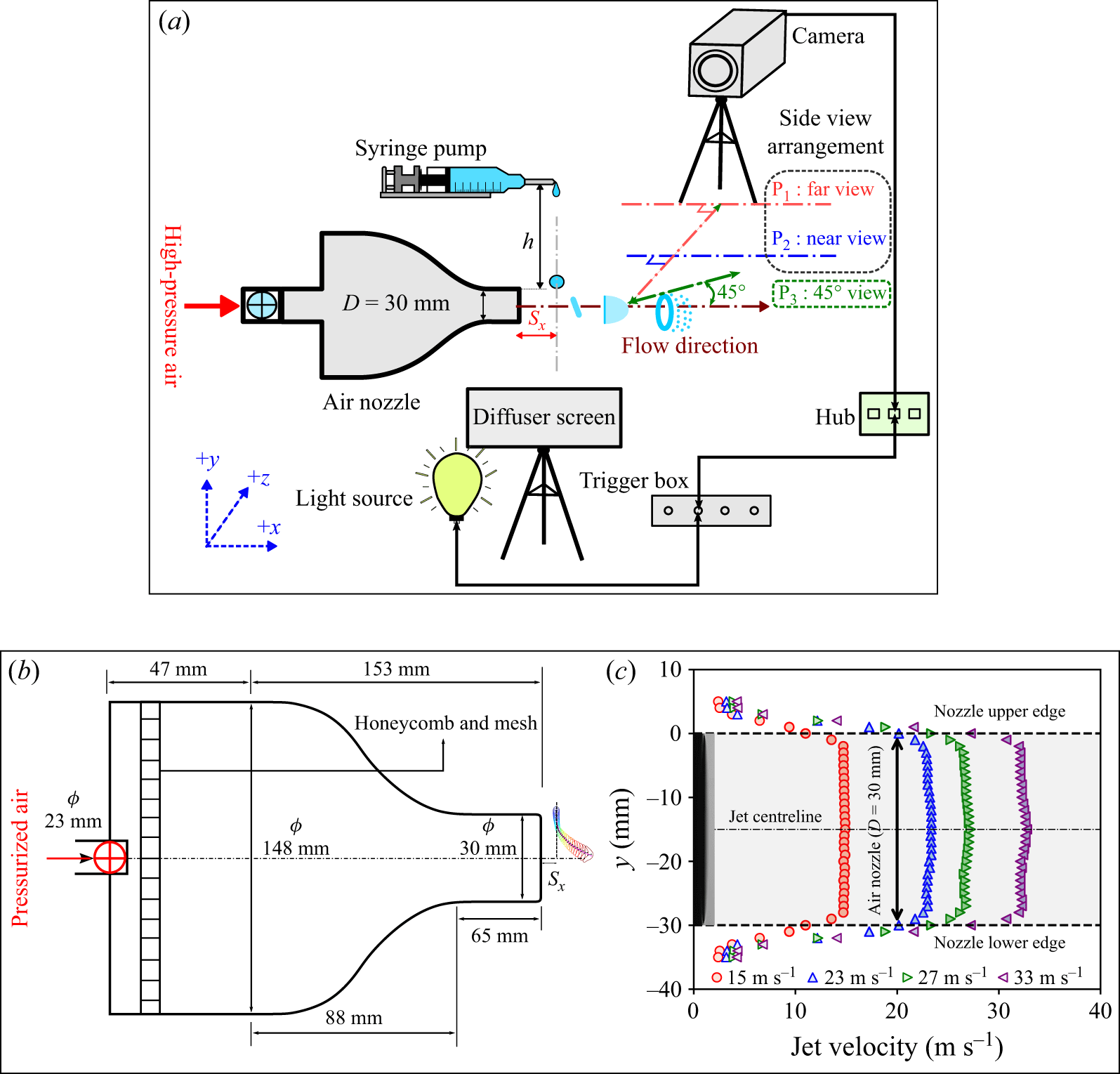
 Sx=10
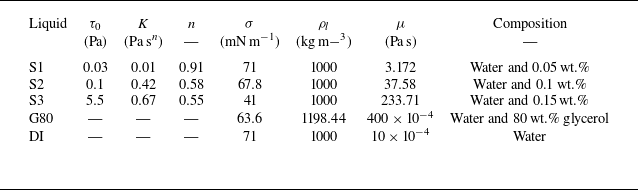
 μ
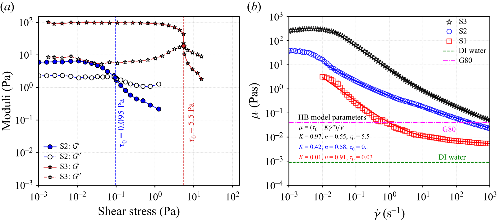
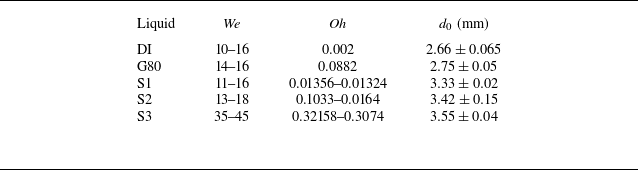

 P1
 We≈13.27
 Oh=0.002
 We≈14.88
 Oh=0.0896

 P2
 We≈13.21
 Oh=0.014
 We≈15.77
 Oh=0.11
 We≈41.08
 Oh=0.31
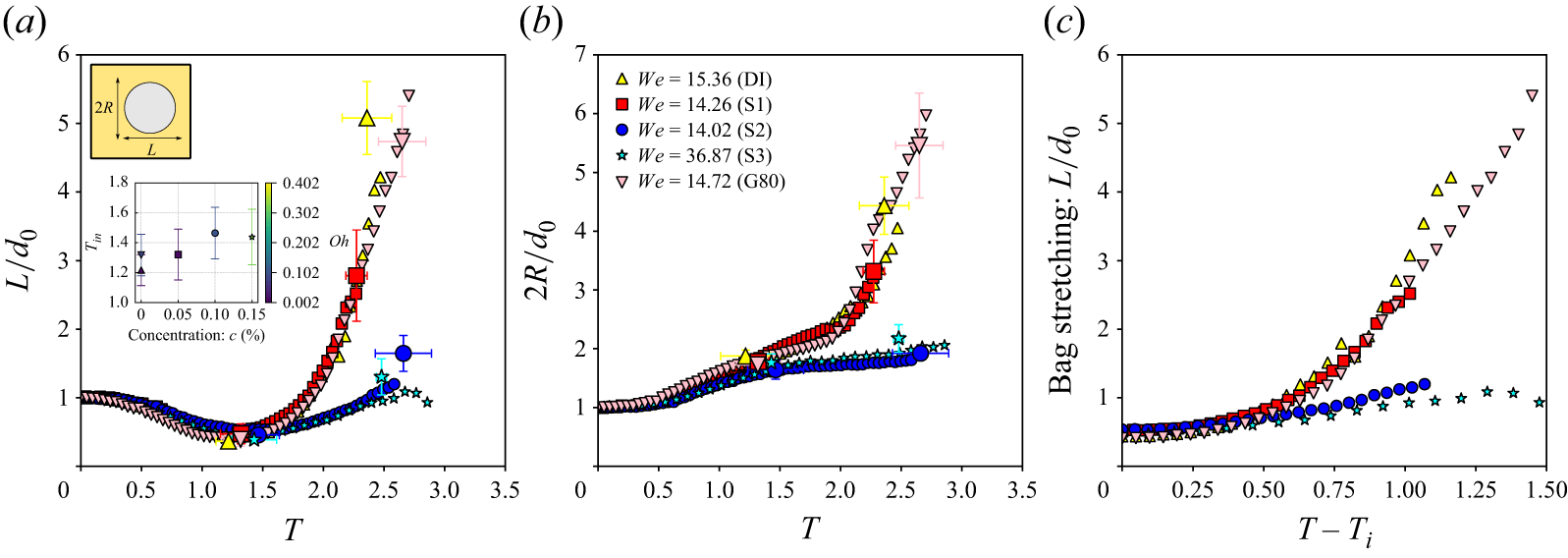
 Tin
 c
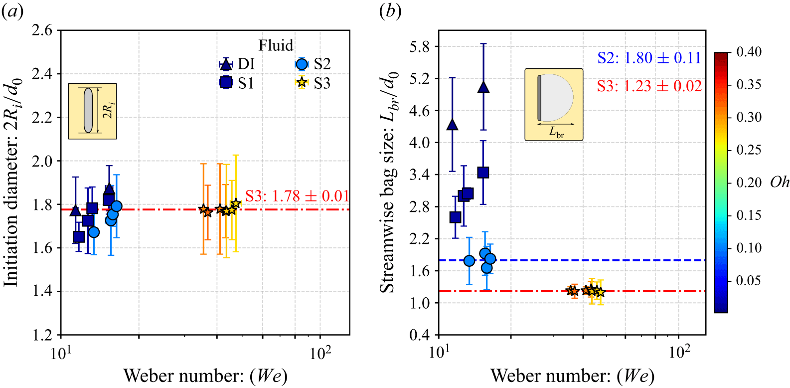
 Oh
 Oh
 We

 45∘
 We≈15
 We≈15.45
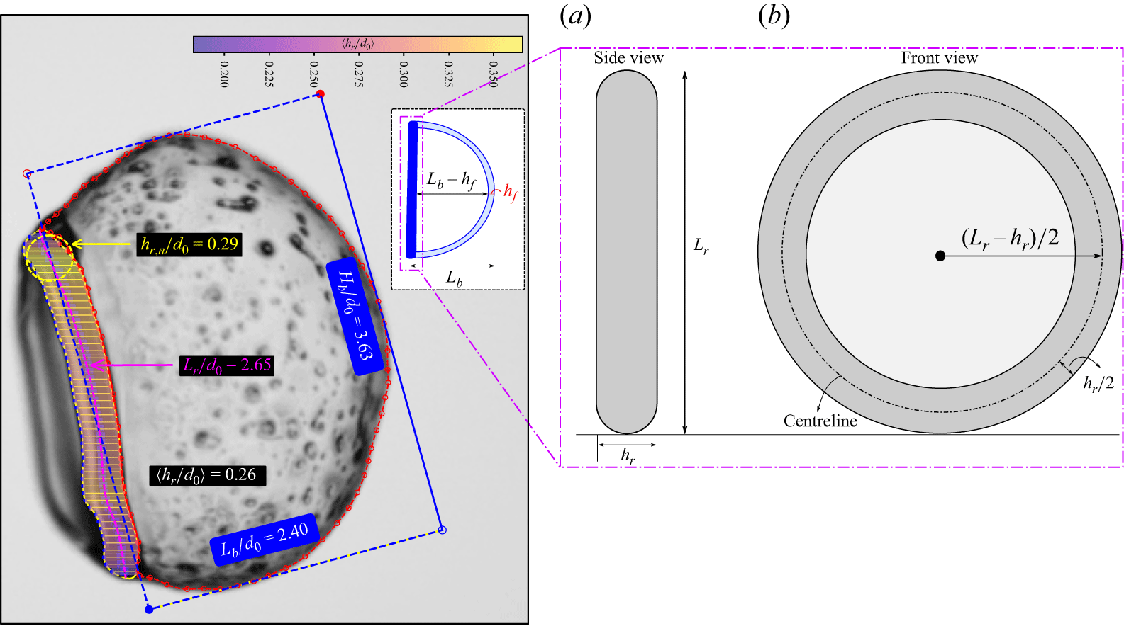
 We=13.21
 hf
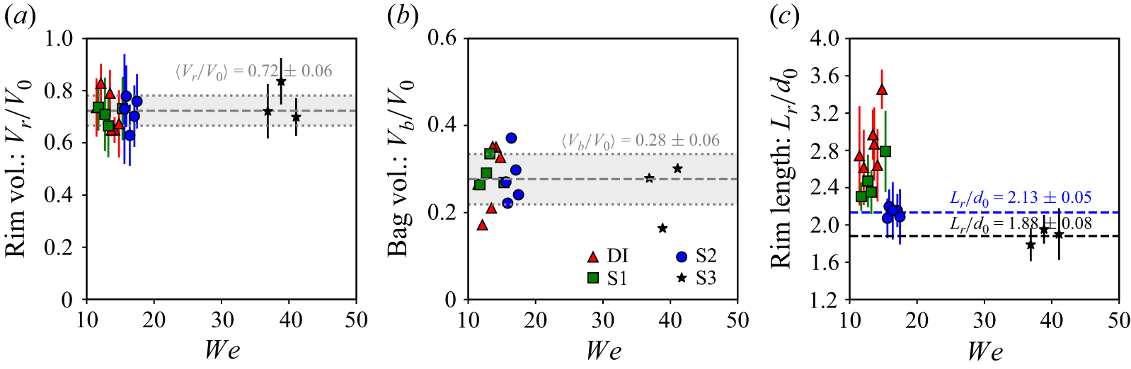
 We

 We
 We

 c=0
 c=0.05
 %
 c=0.1
 %
 c=0.15
 %
 c=0%
 c=0.15
 %

 We≈16.45
 Oh≈0.1

 45∘
 We≈15.45
 t
 0.25

 We=13.21
 We=15.86
 We=41.08
 T=0

 We=12.71
 17.46
 43.15
 λrr
 b

 We
 We
 ×
 λrr/d0
 ×
 Oh

 We=13.21
 We=13.65
 We=36.87
 n
 n=4
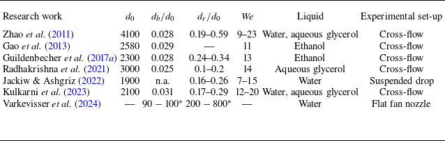

 We=15.31
 Oh=0.013
 We=15.31
 Oh=0.1
 We=36.87
 Oh=0.32
 dn
 dr
 Lr

 We
 Oh
 λRT
 We
 We

 L/d0
 2R/d0
 Wemean=13.33
 T
 95%

 2Ri/d0
 Lbr/d0
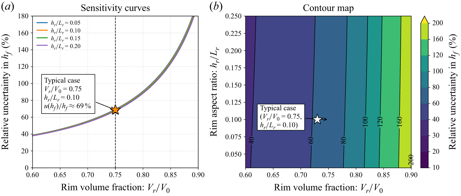
 Lr
 hr
 Lb
 hr/Lr
 Vr/V0
 hr/Lr
 Vr/V0=0.75
 hr/Lr=0.10



