




No CrossRef data available.
Rising Inequality and the Politics of Redistribution in Affluent Countries
Published online by Cambridge University Press: 26 August 2005
Abstract
We use data from the Luxembourg Income Study to examine household market inequality, redistribution, and the relationship between market inequality and redistribution in affluent OECD countries in the 1980s and 1990s. We observe sizeable increases in market household inequality in most countries. This development appears to have been driven largely, though not exclusively, by changes in employment: in countries with better employment performance, low-earning households benefited relative to high-earning ones; in nations with poor employment performance, low-earning households fared worse. In contrast to widespread rhetoric about the decline of the welfare state, redistribution increased in most countries during this period, as existing social-welfare programs compensated for the rise in market inequality. They did so in proportion to the degree of increase in inequality, producing a very strong positive association between changes in market inequality and changes in redistribution. We discuss the relevance of median-voter theory and power resources theory for understanding differences across countries and changes over time in the extent of compensatory redistribution.Lane Kenworthy is an associate professor in the Department of Sociology at the University of Arizona (lane.kenworthy@arizona.edu). Jonas Pontusson is a professor in the Department of Politics at Princeton University (jpontuss@princeton.edu). Earlier versions of this paper were presented at the Conference of Europeanists (March 2002), a workshop on the Comparative Political Economy of Inequality at Cornell University (April 2002), the annual meeting of the Society for the Advancement of Socio-Economics (June 2002), and a seminar at the Center for European Studies, Harvard University (December 2003). For criticisms and suggestions the authors thank Richard Freeman, Janet Gornick, Alex Hicks, Torben Iversen, Larry Kahn, Tomas Larsson, Jim Mosher, Nirmala Ravishankar, David Rueda, Tim Smeeding, John Stephens, Michael Wallerstein, Christopher Way, Erik Wright, and the Perspectives on Politics reviewers.
Information
- Type
- Research Article
- Information
- Copyright
- © 2005 American Political Science Association
Inequality has emerged as a major theme in the comparative study of advanced capitalist political economies over the last decade. The comparative political economy literature of the 1970s and 1980s focused on explaining cross-national variation in macroeconomic management, incomes policy, industrial policy, and macroeconomic outcomes such as growth, unemployment, and inflation. The parallel comparative welfare state literature focused on understanding differences across countries in public social expenditures, institutional arrangements, and principles of eligibility. Neither literature paid much attention to distributive outcomes. As David Bradley and colleagues suggest, this was due largely to lack of good, comparable data on the distribution of earnings and incomes.1
Bradley et al. 2003, 195–96.
Curiously, the view that rising inequality is the big story, and that this trend derives from the changing dynamics of labor markets, persists despite the fact that the available data show that earnings differentials have remained stable or even declined in many countries. In this paper, we review existing literature and present new data on inequality trends in the affluent OECD countries. Our data derive from the Luxembourg Income Study (LIS) and refer to income inequality among working-age households. Largely descriptive and conceptual, the paper makes three contributions to the comparative study of inequality.
First, we map trends in the distribution of gross market income, that is, the distribution of income before taxes and government transfers. In contrast to data on the distribution of earnings among employed individuals, this measure of inequality takes into account the distribution of employment across households. Using income data for working-age households rather than earnings data for individuals, we indeed observe a significant increase in inequality in most OECD countries. Moreover, the pattern of cross-national variation is not what one might have expected: the United States is not alone in having experienced rapid growth of market inequality. We also observe comparatively large increases in household inequality in the Nordic countries—traditional paragons of egalitarianism. These observations point to the crucial importance of (differential) access to employment as a source of income inequality.
Second, we examine changes in the redistributive effects of taxation and income transfers to households. The extensive literature on “welfare state retrenchment” that has emerged over the last decade seems to imply that welfare states have become less redistributive. Our data, to the contrary, show that most welfare states became more redistributive in the 1980s and 1990s. Welfare states have not compensated completely for the rise in inequality of market income among working-age households, but most have done so to some degree. By and large, welfare states have worked the way they were designed to work. It is markets, not politics, that have become more inegalitarian.
Third, we contribute to the ongoing debate about the relationship between market inequality and redistribution, specifically the debate about the utility of the median-voter theorem proposed by Allan Meltzer and Scott Richard.2
Meltzer and Richard (1981).
We present our main findings in three sections, corresponding to the contributions outlined above: we look first at trends in market inequality, then at trends in redistribution, and finally at the relationship between market inequality and redistribution. In addition, we append an explanation (and justification) of how we measure inequality and redistribution, along with data based on alternative measures.
One measurement issue merits discussion at the outset: whether change in inequality should be measured in absolute terms or in percentage terms, relative to initial levels. This question arises when we compare changes in market inequality over time and also when we compare redistribution at any given point in time. We adopt an absolutist approach to measuring change in inequality. Our main findings are similar with change measured in percentage terms, but in one instance (noted below) the association between different variables is more pronounced with change measured in absolute terms.
As we state in the appendix, absolute measures of change are easier to interpret than relative measures and also more substantively sensible. Suppose that market inequality, measured by decile ratios or Gini coefficients, increases in two countries by the same amount from one point in time to another.3
Ranging from zero to one, the Gini coefficient represents the proportion of total income that would have to be redistributed to achieve perfect equality (higher numbers thus signify greater inequality).
The question of the relative salience of household income versus individual income for the politics of inequality lies beyond the purview of this paper.4
A recent paper by Iversen and Rosenbluth (2004) argues that households have become less relevant to political preference formation as marital instability has increased in the affluent countries.
Trends in Market Inequality
Almost all of the recent literature by political scientists on market inequality, either as a dependent or an independent variable, relies on an unpublished, continuously updated OECD dataset on gross (pretax) earnings from employment for individuals who are employed full-time.5
Figure 1 summarizes trends in earnings inequality over the 1980s and 1990s in all countries for which the OECD reports comparable earnings data. The OECD dataset only enables us to measure inequality by decile ratios. As in most of the existing literature, the measure of inequality presented in figure 1 is the 90/10 ratio, that is, the ratio of the earnings of someone in the 90th percentile to the earnings of someone in the 10th percentile of the earnings distribution. The countries are ordered according to the absolute amount of change in inequality, measured as the most recent observation minus the earliest observation.
P90/P10 ratios for earnings among full-time employed individuals, 1979–2000
The OECD data on individual earnings cover different time periods for different countries. Note that the Danish time series ends in 1990, the Belgian time series in 1993, and the Canadian time series in 1994, and the Belgian, Danish, Italian, and Swiss data cover periods of ten years or less. Comparing countries in terms of total change in earnings inequality over time periods of different duration is obviously questionable. However, the country rankings based on average annual change in 90/10 earnings ratios are very similar to those in figure 1, and the correlation between total change and average annual change is 0.94 (see appendix). Keeping in mind the limits of some of the country data, figure 1 indicates that earnings inequality increased in nine out of fifteen countries in the 1980s and 1990s, but held steady or declined somewhat in the other six countries.
Consistent with conventional expectations, figure 1 suggests that rising earnings inequality is first and foremost a characteristic of liberal market economies as conceptualized by the “varieties of capitalism” school:6
the United States, New Zealand, the United Kingdom, Australia, and Canada. Though the extent of inegalitarian trends varies considerably among them, all liberal market economies have experienced significant increases in earnings inequality. The United States stands out as the country in which earnings inequality has grown most dramatically in absolute terms. (Relative to initial levels, the increase in earnings inequality in New Zealand from 1984 to 1997 was nearly as large as the increase in the United States from 1979 to 2000.) We also observe rising earnings inequality in the Netherlands, Sweden, Italy, and Germany; however, inegalitarian trends generally appear to have been more muted in Europe's “social market economies” than in the liberal (Anglo-American) market economies. This also holds for Japan.7Estevez-Abe, Iversen, and Soskice 2001 treat stable wage distributions as a coordinate of the distinctive skill profiles of “coordinated market economies.”
Many scholars have attempted to explain cross-national variation in earnings inequality trends since the 1970s. Labor economists typically attribute the rise in earnings inequality to changes in relative supply and demand for more- or less-skilled labor, but concede that such factors do not adequately explain the observed cross-national variation.8
Students of comparative political economy have recently explored the role of labor market institutions in a more systematic fashion. Some authors emphasize that more centralized or coordinated forms of wage bargaining generate wage compression;9 others point to the bargaining power of unions, measured by union density, as the key variable.10 David Rueda and Jonas Pontusson also show that countries with large public sectors tend to have more egalitarian earnings distributions.11Rueda and Pontusson 2000. The main issue of contention in this literature concerns the effects of government partisanship under different institutional arrangements. While Pontusson, Rueda, and Way (2002) argue that centralized bargaining renders government partisanship less to salient to the relative fortunes of low-wage workers, Beramendi and Cusack (2004) suggest that centralization accentuates the impact of government partisanship.
All this might suggest that market forces have impelled earnings inequality to rise across the affluent OECD countries, but that centralized wage bargaining, strong unions, and large public sectors have muted the effects of these forces in some countries. Alternatively, changes in institutions might be seen as a source of rising earnings inequality. In particular, union decline and public-sector retrenchment (or restructuring) are rather consistently associated with changes in earnings inequality on a cross-national basis.12
Pontusson 2005, chap. 3. By contrast, existing measures of centralization (or coordination) of wage bargaining do not show any secular trends that might be invoked to explain rising earnings inequality (see, for example, Golden, Wallerstein and Lange 1999).
Our goal is not to discuss the determinants of earnings inequality, but rather to point out that the individual earnings data presented in figure 1 capture only one dimension of labor market trends and do not provide the basis for a comprehensive assessment of the extent to which inequality has increased in different OECD countries. In particular, these data fail to capture the distributive effects of unemployment, underemployment, and labor force exit. The analytical problem that unemployment (or nonemployment) poses in this context is not simply that earnings-based measures of inequality exclude the unemployed segment of the labor force. The problem goes deeper because job losses during economic downturns are not distributed equally across the wage distribution. Evidence indicates that employers are more likely to fire unskilled (low-paid) than skilled (high-paid) workers during cyclical downturns. Employers are reluctant to fire skilled workers because it is difficult and costly for them to reacquire the skills that such workers embody when demand picks up again. Since low-wage workers disproportionately drop out of the employed labor force, increased unemployment tends to reduce earnings inequality among employed workers during economic downturns. Surely we ought not interpret this to mean that unemployment promotes equality.13
With 90/10 earnings ratios as the dependent variable, Rueda and Pontusson (2000) report a negative (but not statistically significant) coefficient for the current-year rate of unemployment. By contrast, Pontusson, Rueda, and Way (2002) report a positive (and significant) coefficient for the average rate of unemployment over the preceding five years. The latter result suggests that persistently high levels of unemployment undermine the relative bargaining power of low-wage (unskilled) workers.
In addition, the underlying data used to calculate the 90/10 earnings ratios presented in figure 1 are, except in the case of Norway, restricted to full-time workers. Part-time workers earn considerably less per hour than full-time workers in all OECD countries, but they tend to do better relative to full-time workers in countries where wages among full-time workers are more compressed.14
OECD 1999, 24; Pontusson 2005, chap. 3.
OECD 2004, 310–11.
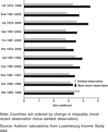
For eleven OECD countries, data from the Luxembourg Income Study enable us to trace the evolution of Gini coefficients for gross market income among working-age households over the 1980s and 1990s, with “working-age households” defined as households headed by individuals aged 25–59. Figure 2 shows the earliest and most recent available Gini coefficients, with countries ordered by the magnitude of absolute change from the earliest to the most recent observation. Here too, the calculations refer to country-specific time periods.16
In particular, note that the figures for Finland, Australia, Denmark, and Switzerland refer to shorter time periods—and, in the cases of Australia and Switzerland, to earlier time periods—than the figures for the other seven countries. Measuring change on average annual basis would render the numbers more directly comparable, but we should be wary of extrapolating beyond the specific time periods covered by the data presented in figure 2. For instance, the increase of household inequality that we observe in Finland from 1987 to 2000 reflects the deep economic crisis that Finland underwent in the 1990s, and there is every reason to believe that Finland did not experience a similar increase of household inequality in the 1980s. As a practical matter, the correlation between total change and annual average change is again quite close (0.93); annualizing change does not significantly affect the country rankings shown in figure 2 (see appendix).

Gini coefficients for market income among working-age households, 1979–2000
Figure 2 conveys a strikingly different picture from that of figure 1. The data on household income show an OECD-wide rise in market inequality. The Netherlands is the only exception to this general trend. Equally notable, figure 2 casts new light on the American experience of the 1980s and 1990s. Whereas the dramatic growth of earnings inequality in the United States over the last two decades (see fig. 1) appears to be exceptional, the United States does not stand out when it comes to trends in market inequality among working-age households. More generally, figure 2 provides no support for the proposition that the growth of inequality has been more pronounced in liberal market economies than in social market economies. Quite the contrary, Sweden, Finland, and Norway hold three of the top six positions when the affluent OECD countries are ranked by change in household inequality over this period.
Finland and the Netherlands illustrate the divergence between trends in individual earnings inequality and household income inequality most starkly. In Finland, earnings inequality among full-time employees declined marginally from 1980 to 2001, but household inequality increased sharply from 1987 to 2000. In the Netherlands, by contrast, earnings inequality increased from 1979 to 1999, but household inequality declined over roughly the same period (1983–99).
As we demonstrate in the appendix, the divergence between trends in individual earnings inequality and household income inequality represents a substantive puzzle rather than an artifact of the different properties of Gini coefficients and 90/10 ratios as measures of inequality. Analyzing patterns of labor force entry and exit provides one possible avenue to resolve this puzzle. In particular, the rise in market income inequality in countries that did not experience much increase in earnings inequality might be due to an increase in the share of households with little or no market income. We might reasonably look first to the youngest and oldest labor force participants. Among those aged 50 to 59, increases in early retirement may have contributed, though this form of labor force exit is most prevalent in continental European countries, which were not the countries experiencing the sharpest rise in income inequality.17
Expansion of higher education may have had a similar effect among households headed by individuals aged 25 to 29. It turns out, however, that if we restrict our analysis to households headed by individuals aged 30 to 49, the picture that emerges is essentially the same as that shown in figure 2. In each country the magnitude of increase in inequality is similar for this narrower age group, and the cross-country correlation between changes in market inequality for households with heads aged 25 to 59 and for households with heads aged 30 to 49 is 0.99.Patterns of entry and exit into the labor force are closely related to employment conditions, and employment performance is surely the key to the contrast between Finland and the Netherlands, which, in the 1990s, represent opposite ends of the OECD spectrum in this respect. In Finland the employment rate declined by 14 percentage points from 1990 to 1994, and the rate of unemployment rose from 3 to 17 percent, remaining above 10 percent through the rest of the decade. By contrast, the Netherlands outperformed all OECD countries but Ireland in terms of employment growth in the 1990s, with its employment rate increasing by 10 percentage points between 1990 and 2000 and its unemployment rate dropping from 6 to 3 percent.18
Pontusson 2005, chap. 4.
Other factors must also be considered as we grapple with the differences between the inequality trends shown in figures 1 and 2. Rising household inequality across the affluent OECD countries is partly a result of changes in demographics and household structure, in particular, the growing incidence of single-adult households20
Bradley et al. 2003; Esping-Andersen 2005; Kenworthy 2004; Kenworthy (forthcoming).
Burtless 1998; Esping-Andersen 2005; Kenworthy 2004; Kenworthy (forthcoming).
To decompose changes in household inequality along these lines is a complicated task, well beyond the scope of this paper. Suffice it to say that, aside from employment opportunities for low-income households, marital instability and its concomitant, single-headed households, constitute the most obvious factor for explaining the cross-national variation in inequality trajectories shown in figure 2. The Nordic countries are distinguished by high divorce rates.22
With respect to timing, however, the employment crisis experienced by the Nordic countries, especially Sweden and Finland, in the early 1990s provides a more powerful explanation of the rise of household inequality in these countries.23In a similar vein, Mishel, Bernstein, and Boushey (2003, 78–82) show convincingly that household-compositional accounts of the rise of household inequality falter on the issue of timing: the negative effects of changes in household type were most pronounced in the 1970s, yet income growth across quintiles was more even distributed during this decade than during the subsequent two decades.
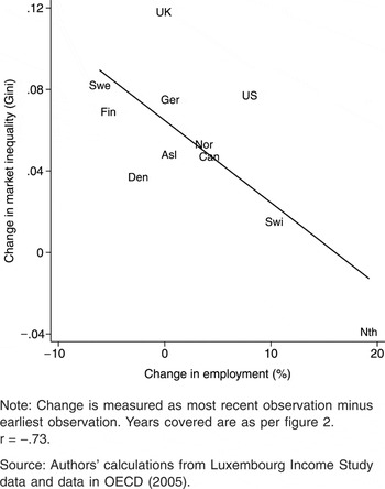
Figure 3 illustrates the significance of employment for trends in household inequality by plotting changes in Gini coefficients for household market income against changes in the employment rate (the employed as a percentage of the population aged 15 to 64) for each country.24
Note that change in the employment rate is here measured over the same (country-specific) time periods as change in Gini coefficients. The fact that the data refer to different time periods for different countries does not affect the association between the two variables shown in figure 3.

Change in market income inequality by change in employment rates, working-age households, 1979–2000
Regressing change in Gini coefficients for household market income inequality on change in employment rates and change in individual earnings inequality, from the earliest to the most recent observations reported in figures 1 and 2, yields the following results (t-statistics in parentheses):

We should not put too much stock in a regression analysis based on only eleven observations and poorly matched data for household and earnings inequality, but these results are certainly suggestive: trends in employment and earnings inequality together provide leverage on the question of why income inequality among working-age households has grown more in some countries than in others. The standardized coefficients are −0.82 for change in employment rates and 0.42 for change in earnings inequality, suggesting that employment is the more important variable. In a similar vein, Kenworthy has shown that from the mid-1980s to the mid-1990s the effects of changes in employment and, to a lesser extent, earnings inequality were larger and more consistent than the effects of changes in the incidence of single-adult households.25
Kenworthy 2004, 30.
Employment and family structure need not be construed as competing explanations for rising household inequality. Single-headed households are significant in this context precisely because their ability to compensate for rising earnings inequality by increasing employment is constrained. As Jelle Visser and Anton Hemerijck have shown, much of the Dutch “jobs miracle” in the 1980s and 1990s involved an increase in part-time employment among married women.26
Visser and Hemerijck 1997, 29–35.
The implication of the evidence presented above is that employment contractions disproportionately hurt the employment opportunities and hence the fiscal well-being of low-income households; conversely, job growth disproportionately benefited low-income households. Again, low-income households in the Netherlands and, to a lesser extent, the United States and other liberal market economies appear to have compensated for falling relative earnings by increasing their employment—more household members work, or those that do, work more. Low-income households appear to have been less able—or less willing—to engage in this type of compensatory behavior in those countries for which we observe little or no increase in individual earnings inequality but a significant increase in household inequality (Finland, Norway, Denmark, and Switzerland) or, as in the Swedish case, a larger increase in household inequality than in earnings inequality.
The existing literature points to two explanations for “compensatory employment” in some countries but not others. On the demand side, a combination of wage compression through centralized wage bargaining and high payroll taxes may weaken relative demand for low-wage workers in the more egalitarian social market economies of northern Europe.27
Note that this is an argument about relative demand for different kinds of labor rather than overall demand. Kenworthy (2003, 2004) reports some employment effects of earnings compression, but finds that other labor market institutions and policies matter as much or more to cross-country variation in employment performance. See also Blau and Kahn 2002; Iversen and Wren 1998; Nickell and Layard 1999; Pontusson 2005; and Scharpf 2000.
Trends in Redistribution
The LIS database also allows us to examine the redistributive effects of taxation and transfer payments by governments. At the end of the day, what matters to people is not market income, but rather disposable income, that is, income after taxes and transfers. Some analysts measure redistribution as the difference between Gini coefficients computed for disposable household income and Gini coefficients computed for gross market household income expressed in percent of Gini coefficients for gross market household income.29
We believe that the absolute difference between disposable-income and market-income Gini coefficients represents a better and more easily interpretable measure of redistribution.30We also report percentage measures of redistribution in the appendix.
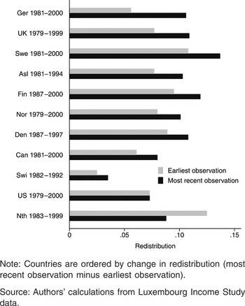
Figure 4 provides data on the reduction in Gini coefficients brought about by taxes and transfers in our 11 countries in the early 1980s (later for Denmark and Finland) and the late 1990s (earlier for Switzerland and Australia). As with figure 2, the data are restricted to working-age households. The largest government transfer program, pensions, is thus excluded from consideration. This analysis also does not take into account the redistributive effects of the public provision of services, such as education and health care, despite the fact that, services are a critical component of the welfare states of many affluent countries.31
Services do not alter the distribution of income per se, but to the extent they are provided at low or no cost and are universally available, services are equivalent to a flat-rate benefit given to each household, which reduces the degree of consumption inequality. Unfortunately, the LIS data do not include information on the value of such services.32 Thus, in terms of cross-national comparison, the data in figure 4 understate the degree of redistribution in relatively service-intensive welfare states, most notably the Nordic ones.
Redistribution: Gini coefficients for market income minus Gini coefficients for disposable income, working-age households, 1979–2000
Our main interest concerns trends in redistribution. The countries in figure 4 are ordered by change over time (from larger to smaller increases in redistribution). Strikingly, almost all welfare states became more redistributive in the course of the 1980s and 1990s. As with the data on market inequality, the Netherlands stands out as the major exception to the general trend. The Netherlands is the only country in which we observe any reduction in the redistributive effect of taxes and transfers—and the reduction in this case is remarkably large.
Pooling LIS observations for working-age households for 14 countries (for a total of 59 observations) and controlling for the size of the welfare state, Bradley and colleagues show that the share of cabinet portfolios held by Left parties had a significant positive effect on levels of redistribution, measured as the percentage reduction in Gini coefficients brought about by taxes and transfers.33
They find that union density, an alternative measure of working-class mobilization, also had a strong positive effect on levels of redistribution. Their cabinet share measure is cumulative, based on all years from 1946 to the year for which redistribution is observed. Thus their results for government partisanship should be taken to mean that countries in which Left parties have participated in government over extended periods of time tend to have more redistributive tax and transfer systems. Though Bradley and colleagues' analysis is persuasive, government partisanship does not seem to explain the general tendency for redistributive effects to increase.34The fact that redistribution is measured relative to market inequality poses a potential problem for Bradley and colleagues' analysis or, at least, for the aforementioned interpretation of their results. Lower levels of market inequality are, by definition, associated with higher levels of redistribution when redistribution is measured in this manner. Thus the observed (positive) effect of leftist cabinet shares on redistribution could be due to a (negative) association between leftist cabinet shares and market inequality. This issue is even more relevant to the effects of unionization on market inequality. It should also be noted Bradley and colleagues' analysis includes Belgium, France, and Italy. The LIS dataset only allows us to compute household inequality for “net market income” (that is, income after taxes), not “gross market income,” for these countries; therefore they are not included in our analysis.
Garrett 1998, 60.
More generally, the evidence presented in figure 4 provides support for Paul Pierson's emphasis on the resilience of welfare states in the face of globalization or fiscal and demographic pressures and calls into question the common notion that recent tax and social policy reforms in the affluent countries have been uniformly and extensively regressive.36
It should be noted, though, that the increases in redistribution that we observe in the LIS data are almost entirely attributable to the effects of transfer payments. In most countries, the contribution of taxation to redistribution declined over this period.37Calculations are available from the authors upon request.
Allan and Scruggs 2004. See also Korpi and Palme 2003.
How can we reconcile such evidence of welfare state cutbacks with the data on trends in redistribution? The obvious explanation for this puzzle is that labor market developments—rising joblessness among unskilled workers and rising earnings inequality—have rendered more households eligible for unemployment compensation and other transfer programs, and that increasing claims on these programs by low-income households have rendered government spending more redistributive, even as eligibility criteria have been tightened and benefit levels reduced.40
Indeed, it seems quite clear, especially with respect to unemployment insurance, that benefit cuts have been driven partly by increases in eligible recipients. See Huber and Stephens 2001.
Ploug 1999, 83, 95. See also Marklund and Nordlund 1999, 29.
Our calculations from LIS data.
The bottom line is that there are two different paths to increased redistribution. One path involves new policy initiatives or policy changes aimed at redistributing income, such as easing eligibility restrictions or increasing replacement rates. The second path involves a more or less automatic compensatory response by existing welfare states to rising market inequality. In the 1980s and 1990s, most affluent OECD countries seem to have been on the second path.
The Effect of Market Inequality on Redistribution
The median-voter model elaborated by Meltzer and Richard43
informs much recent discussion of the relationship between market inequality and redistribution.44See, for example, Alesina and Glaeser 2004, 57–60.
See also Romer 1975.
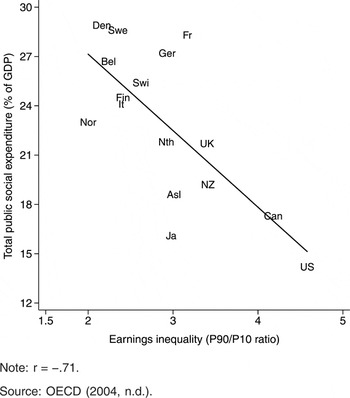
The Meltzer-Richard model implies that countries with more unequal distributions of market income should exhibit higher levels of redistributive spending than countries with less unequal distributions. As commonly noted, this prediction is not borne out by the data for the OECD countries. Plotting levels of total government spending on social transfers and services against levels of earnings inequality among full-time employees (fig. 5), we observe an associational pattern quite the opposite of what the Meltzer-Richard model leads us to expect: countries with more egalitarian earnings distributions tend to have larger welfare states than countries with more inegalitarian wage structures. Torben Iversen and David Soskice refer to this pattern as the “paradox of redistribution.”46

Total public social expenditures in percent of GDP in 2000 by most recent observation of earnings inequality among full-time employed individuals
Does figure 5 invalidate the Meltzer-Richard model? As we have seen, it is problematic to use individual earnings inequality as a proxy for market inequality. Also, Meltzer and Richard present their model as an explanation of the size of government, but their model is really meant to explain redistribution. Meltzer and Richard in effect assume that all government spending takes the form of transfers to individuals or households and that all spending is (equally) redistributive. To test their model empirically, it would be more appropriate to examine redistribution rather than spending. The LIS data on market income inequality and redistribution among working-age households are in fact more consistent with the predictions of the Meltzer-Richard model than are the data presented in figure 5. Before turning to the LIS data, let us consider some objections to and extensions of the Meltzer-Richard model.
Clearly, the Meltzer-Richard model rests on a simple, perhaps simple-minded, view of politics. First, it assumes that elections determine redistributive policy and that electoral politics are only about redistributive policy. Voters are assumed to have well-defined, single-peaked preferences over redistribution that derive from their income relative to the mean income. Voters are also assumed to be fully informed about the policy choices before them. The “real world” of politics rarely, if ever, conforms to these assumptions. Second, the Meltzer-Richard model views political parties as motivated simply by the desire to win elections. The extensive literature demonstrating that the partisan composition of governments affects the extent and character of the public provision of social welfare calls this view into question.47
Recent work demonstrating the persistence of partisan effects in the 1980s and 1990s includes Allan and Scruggs 2004, Korpi and Palme 2003, and Kwon and Pontusson 2004.
The core propositions of the Meltzer-Richard model alone do not provide an adequate basis for understanding the politics of redistribution. The more interesting question is whether, in the context of other relevant considerations, they shed some light on the politics of redistribution. In addition, the model can easily accommodate inequality of political influence insofar as such inequality derives from the fact that low-income earners are less likely to vote than high-income earners. As Phillip Nelson points out, the income of the median voter should not be confused with the median income.49
For the United States, the ratio of the median household income to the mean household income averaged 0.82 in the 1970s and 1980s. With household income weighted by the number of adults in each household, however, the ratio of the household income of the median voter to the mean household income averaged 1.02.50Ibid., 189.
Quite appropriately, quantitative comparative political economy literature commonly invokes the Meltzer-Richard model to justify the hypothesis that voter turnout has a positive effect on redistributive government spending (for example, Iversen and Cusack 2000; Franzese 2002).
With regard to the motivations of political parties, the observation that parties cater to the distributive interests of their core constituencies and possibly also have ideological commitments to certain policies surely does not mean that they do not care about winning elections. Median-voter logic and partisanship need not be construed as mutually exclusive. In Geoffrey Garrett's formulation, we should expect governing parties of different political persuasions to pursue distinctive distributive policies so long as their pursuit of such policies does not threaten their prospects of reelection.52
Garrett 1998. See also Strom 1990.
Proceeding from the same basic assumptions as Meltzer and Richard, Moene and Wallerstein attempt to resolve the “paradox of redistribution” by pointing out that government spending not only redistributes income, but also provides insurance.54
The core proposition of their extension of the Meltzer-Richard model is that demand for insurance increases with income, holding risk (for example, the threat of unemployment or disability) constant.55Iversen and Soskice 2001 develop a similar insurance model of demand for public welfare provision, emphasizing that risk exposure varies depending on skill specificity.
The power resources approach advanced by John Stephens and Bradley and colleagues represents an obvious alternative solution to the “paradox of redistribution.”57
In the power resources view, the negative association between earnings inequality and welfare spending across countries derives from the influence of working-class mobilization on both. Strong unions and Left parties compress the wage distribution and also boost redistributive social spending. In other words, there is no direct causal relationship between market inequality and welfare spending.As indicated above, our main goal here is to recast the empirical basis of this debate by measuring inequality on a household basis—thus incorporating the effects of differential access to employment—and by focusing directly on the redistributive effects of public policy (tax policy as well as spending policy). To be consistent with our previous discussion and to side-step the “distortion” of redistributive effects created by generous public pensions (see appendix), our analysis remains restricted to households headed by people of working age. Excluding the retired population is obviously problematic from the point of view of testing median-voter theory, since retired people do vote, often more than working-age people. This is also a problem, however, for those who use individual earnings inequality as a proxy for market inequality.58
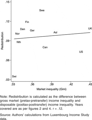
Based on the most recent LIS observations available for eleven countries, figure 6 plots redistribution, measured as the (absolute) difference between Gini coefficients for gross market income and for disposable income, against levels of market inequality, measured by Gini coefficients for gross market income. We see a positive association between market inequality and redistribution among the Nordic and continental European countries, but, overall, figure 6 clearly does not support the Meltzer-Richard model. On the other hand, we no longer observe a pattern of association that runs counter to the Meltzer-Richard model. The “paradox of redistribution” effectively disappears when we measure market inequality and redistribution in the fashion proposed here.

Redistribution by market income inequality, working-age households, most recent LIS observations
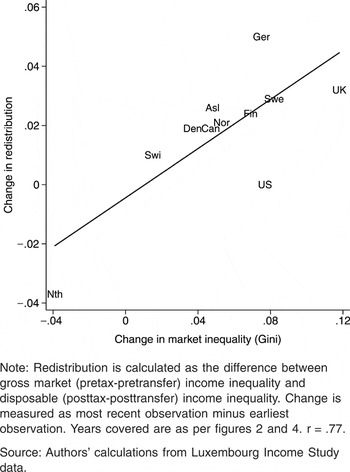
Figure 7 plots changes in redistribution against changes in household market inequality over the 1980s and 1990s. Based on figures 2 and 4, figure 7 again uses the earliest available circa 1980 observation and the most recent available observation for each country. Here, we do observe the pattern of association that the Meltzer-Richard model predicts: in general, redistribution increased more in countries that experienced larger increases in market inequality in the 1980s and 1990s.59
This association is weaker, though still consistently positive, if change in inequality and change in redistribution are measured in percentage, rather than absolute, terms. The percentage-change data are shown in the appendix.

Change in redistribution by change in market income inequality, working-age households, 1979–2000
It would be a mistake to interpret figure 7 as evidence for the political process posited by the Meltzer-Richard model. It would surely be a stretch to say that rising market inequality led median voters in the affluent countries to opt for more redistributive parties and policies in the 1980s and 1990s. As suggested above, the observable increases in redistribution should be seen mainly as a more-or-less automatic response to inegalitarian labor market developments by existing welfare states. Nevertheless, we also caution against an overly path-dependent view of compensatory redistribution. In many countries, income taxation became less progressive, and various social transfer programs were in fact scaled back over this period. But neoliberal politicians often advocated more extensive tax reforms and cutbacks than were in fact undertaken. It seems quite reasonable to suggest, in the spirit of Meltzer-Richard, that in the context of rising market inequality the policy preferences of median voters constrained this neoliberal offensive.
Taken together, figures 6 and 7 suggest that the logic of the Meltzer-Richard model captures a dynamic that liberal democracies have in common, but also that there are important cross-national differences in “tastes for equality” or beliefs about the proper role of government60
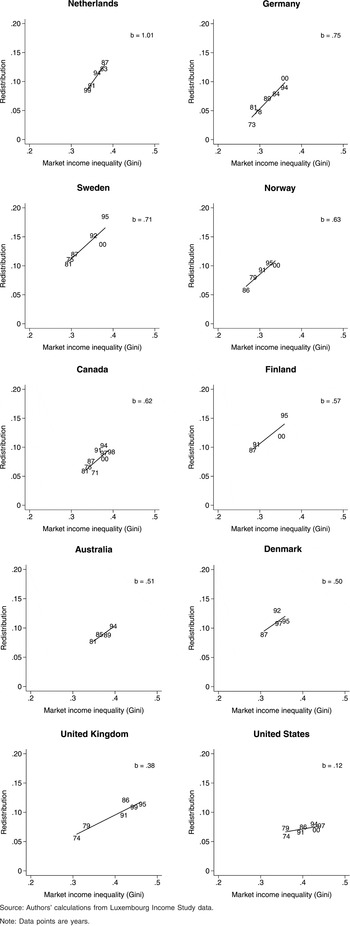
that cannot be explained in terms of the effects of income distribution on the policy preferences of the median voter. Figure 8 further illustrates both of these points. The LIS database provides at least four different observations for ten countries and includes observations from the 1970s for some of these countries. For each of these ten countries, figure 8 presents a scatterplot of the over-time relationship between household market income inequality and redistribution. It also shows the coefficient (b) obtained by regressing redistribution on market inequality.61As above, the data are restricted to working-age households and redistribution is measured as the difference between Gini coefficients for gross market income and disposable income.

Redistribution by market income inequality, working-age households, 1970–2000
With the exception of the United States, we observe a relatively strong positive association between market inequality and redistribution in every country. But the slope of the regression line differs markedly across countries. For the United States, the sign of the coefficient is positive, but the line is nearly flat. Followed by Germany, the Netherlands stands out as the welfare state that has been most responsive to—in other words, compensated most fully for—increases (and reductions) in market inequality. Contrary to what the comparative welfare-state literature might lead us to expect,62
For example, Esping-Andersen 1990; Hicks 1999; Huber and Stephens 2001.
What accounts for the “redistribution elasticities” shown in figure 8? Why are some welfare states more responsive to market inequality than others? From the perspective of the Meltzer-Richard approach, voter turnout would seem to be the most obvious determinant of cross-national variation in compensatory redistribution. As Walter Korpi argues, voter turnout can be seen at least partly as a measure of the capacity of unions and labor-affiliated parties to mobilize workers politically.63
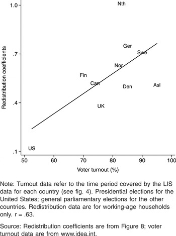
Voter turnout thus emerges as an issue on which median-voter theories and power-resource theories converge. Against this backdrop, figure 9 plots the regression coefficients presented in figure 8 against average turnout in general elections over the country-specific periods covered by our LIS data. Though the fit between the variables is not terribly good, this figure provides some tentative support for the proposition that high turnout produces institutionalized policy commitments, which in turn produce greater responsiveness to increases in market inequality. Perhaps the most important point to take away from figure 9 is that low turnout offers a potentially compelling explanation for why the American welfare state has been so much less responsive to rising market inequality than other welfare states.
Redistribution coefficients by average voter turnout
Figure 9 suggests that voter turnout, treated here as a proxy for the electoral mobilization of low-income workers, conditions the responsiveness of government policy to market income inequality trends. Alternatively, voter turnout and market inequality might be seen as variables that affect redistribution independently. Pooling all available LIS observations, we regressed redistribution on market inequality and voter turnout (in the election immediately preceding each LIS observation).64
The regression model addresses the problem of heteroskedasticity by means of a technique called “robust cluster” (see Bradley et al. 2003). Since there is no single year in common to all countries, the standard (Beck-Katz) procedure for estimating panel-corrected standards could not be used. In addition to the observations shown in figure 8, the regression includes two LIS observations for Switzerland and one observation for Belgium.

Market inequality and voter turnout both appear to be associated with higher levels of redistribution. Clearly, more systematic analysis (controlling for other variables that might affect redistribution) is needed to confirm these results, but our preliminary analysis suggests that the Meltzer-Richard model accurately identifies the distribution of market income and voter turnout as key variables in the politics of redistribution, as distinct from the politics of social insurance. At the same time, our discussion points to a potential synthesis of median-voter and power-resource theories: the median-voter theorem helps us to understand changes in redistribution to the extent that unions, Left parties, or other actors mobilize low-income workers to participate in the political process.
Conclusion
We have used LIS data to examine trends in market income inequality, redistribution, and the effect of market inequality on redistribution in affluent OECD countries in the 1980s and 1990s. Unlike for earnings inequality among full-time employed individuals, for pretax-pretransfer income among households we observe sizeable increases over time in most countries. This development appears to have been driven to a large extent by changes in employment. In countries with better employment performance, low-earning households benefited relative to high-earning ones; in nations with poor employment performance, low-earning households fared worse. In contrast to widespread rhetoric about the decline of the welfare state, redistribution tended to increase in response to the rise in household market inequality. And it did so in proportion to the degree of increase in inequality, producing a strong positive association between changes in market inequality and changes in redistribution.
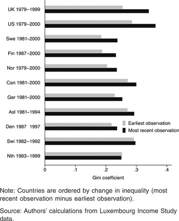
We noted earlier that ultimately people care most about their disposable income, rather than their market income. Figure 10 shows Gini coefficients for disposable income for the eleven countries that appear in figure 2, again with an observation around 1980 and an observation for the most recent available LIS year. Even though redistribution increased in the Nordic countries during the 1980s and 1990s, they nevertheless experienced rising inequality of disposable income. Had it not been for the increase in redistribution in the Nordic countries, inequality of disposable income presumably would have risen even more.

Gini coefficients for disposable income among working-age households, 1979–2000
The charts in figure 8 indicate that the Nordic and continental European welfare states tend to be comparatively responsive to increased market inequality—certainly much more so than their American and British counterparts. But what would happen if European countries were to continue to experience employment difficulties? A long-term decline in employment could potentially pose a threat to the generosity of welfare states even in countries with relatively egalitarian preferences and institutions. The redistributive burden—the tax burden necessary to sustain generous transfer programs—in a country with continuously declining employment might eventually become unsustainable, at least in the public mind, leading to significant cutbacks in such programs. This in turn could cause such a country to shift to a higher “equilibrium” level of disposable income inequality.
While this scenario is not impossible, it has not played out thus far. Although almost all European countries introduced some reductions in the generosity of various transfer programs in the 1980s and 1990s, in most instances those reductions were limited. Moreover, employment rates in the more egalitarian countries have increased in recent years, in some cases substantially. Cross-national diversity in welfare state generosity and inequality of disposable household income is likely to persist and to remain an important subject for research and debate among students of comparative political economy.
Appendix: Data and Measurements
Inequality
Our data for individual earnings inequality are from an unpublished OECD data set,65
which is, to our knowledge, the only source of comparative time-series data for individual earnings. Our data for household income inequality come from the Luxembourg Income Study (LIS) database (http://www.lisproject.org). These data are the best available for cross-country comparison of incomes and income inequality.66Consistent with our focus on labor-market developments as a source of inequality, and following the lead of other researchers,67
Gornick 1999; Bradley et al. 2003; Kenworthy 2004; Kenworthy (forthcoming); Schwabish, Smeeding, and Osberg 2003.
Huber and Stephens 2001, 375.
For example, Mitchell 1991.
For households, we focus on inequality of gross market income (figs. 2, 3, 4 and 6, 7, 8). Gross market income (“market income”) refers to all household income prior to taxes and transfers. It includes earnings from dependent employment and income from self-employment, investments, and gifts. Earnings account for 86–99 percent of total market income across all LIS observations for the eleven countries in figure 2, and inequality of earnings is very closely correlated with inequality of market income among working-age households in the LIS data. Across all LIS observations for those eleven countries (N = 61), the correlation between Gini coefficients for gross earnings and Gini coefficients for market income is 0.98. Based on other data sources, Pablo Beramendi and Thomas Cusack report national averages for earnings from dependent employment as a percent of total market income over the period 1965–95; their figures range from 55 to 79 percent.70
Following conventional practice in studies of the income distribution, we adjust for household size by using an equivalence scale of 0.5.71
Atkinson, Rainwater, and Smeeding 1995; Bradley et al. 2003; Kenworthy 2004; Kenworthy (forthcoming).
Respondents to surveys may overestimate or underestimate their earnings and/or income. To minimize the effect of this, it is standard practice in analyses using the LIS data to top-code and bottom-code the country data sets in calculating household income levels and income inequality. That is, an upper and lower limit for incomes is set based on some multiple and fraction of the median or mean. Any reported incomes above or below these figures are recoded as the limit figures. We follow the official LIS practice of top-coding at 10 times the unequivalized median household income and bottom-coding at 1 percent of the equivalized mean.72
Households reporting a disposable income of zero are dropped.We use P90/P10 ratios to measure inequality of individual earnings (figs. 1 and 5) and Gini coefficients as our measure of income inequality across households (figs. 2, 3, 4, 6, 7, 8, and 10). Our aim is not to provide a direct comparison of the degree of change in individual earnings inequality versus household income inequality. Nevertheless, it would be helpful to have a common metric. While it is not possible to calculate Gini coefficients from the data in the OECD database on individual earnings, it is possible to calculate P90/P10 ratios for household income from the LIS data. However, P90/P10 ratios are dramatically higher when the 10th percentile of the income distribution includes households without any employed adult: for market income, P90/P10 ratios normally range between 0 and 15 (the U.S. figure for 1997 was 12), but the ratio was 61 for Australia in 1994 and 184 for the Netherlands in 1983. The most useful common metric available to us with these data sources is P75/P25 ratios. This measure is strongly correlated both with P90/P10s ratios for individual earnings (r = 0.98) and with Gini coefficients for households (r = 0.92). The data are shown in tables A1 and A2 below. Switching to P75/P25 ratios does not significantly alter the country ranking for over-time trends in either individual earnings inequality or household market income inequality. The common-metric data presented tables A1 and A2 below confirm that household market inequality tends to be greater than and has increased more rapidly than individual earnings inequality.
Individual earnings inequality data using alternative measures

Household market income inequality data using alternative measures

Redistribution
As indicated in the text, we measure redistribution (figs. 4 and 6, 7, 8) by subtracting the Gini coefficient for household gross market income (income before taxes and transfers) from the Gini coefficient for household disposable income (income after taxes and transfers). Many studies of redistribution divide this figure by the Gini coefficient for gross market income, which yields a “percentage” measure of redistribution.73
Our use of an “absolute” measure serves to remove “level effects”—the impact of the level of market inequality on the measure of redistribution—from the analysis. Disregarding level effects is particularly appropriate given that we are primarily interested in exploring changes in redistribution over time.To illustrate this point, consider the Swedish case. From 1981 to 2000, the Gini coefficient for market income among working-age households increased from 0.293 in 1981 to 0.375 in 2000, while the difference between market-income and disposable-income Gini coefficients increased from 0.108 to 0.137. Expressed as a percentage of market-income Gini coefficients, redistribution fell from 36.9 percent to 36.5 percent, but it seems misleading to infer that the Swedish welfare state was less redistributive in 2000 than in 1981. Rather, it is more accurate to say that the Swedish welfare state became more redistributive, but that the increase in redistribution was not sufficient to offset the increase in market inequality. The same logic applies to cross-national comparison. Consider the data for Denmark and the United Kingdom shown in figure 4. In the late 1990s, the absolute effect of taxes and transfers was nearly identical for these two countries: a 0.108 reduction of the Gini coefficient for Denmark and a 0.109 reduction for the United Kingdom. Because the distribution of market income was less unequal in Denmark than in the UK, a percentage measure of redistribution suggests that there was more redistribution achieved in the Danish case (31 percent) than in the British case (24 percent). Leaving aside the question of second-order effects of taxes and transfers,74
See Beramendi 2001.
Measuring change over time
We believe that it is more informative to measure change in inequality in absolute terms (the ending value minus the beginning value) rather than in percentage terms (absolute change divided by the beginning value). Consider, for example, an election in which one party increases its share of the vote from 30 percent to 40 percent while another party increases its share of the vote from 3 percent to 4 percent. We might say that both parties gained 33 percent, but it would be more meaningful to say that one party gained 10 percentage points while the other gained one percentage point. By the same logic, we prefer to say that an increase in the Gini coefficient from 0.300 to 0.400 is equivalent to an increase from 0.200 to 0.300, rather than that it is equivalent to an increase from 0.200 to 0.267. Measuring change in absolute terms is particularly appropriate when we try to gauge the effect of changes in employment on changes in household market income inequality (fig. 3) or the impact of changes in household market income inequality on changes in redistribution (fig. 7). In the language of regression analysis, we have no reason to believe that the effect of a one-unit increase in employment on household inequality (or of household inequality on redistribution) is contingent on the initial level of employment. As noted in the text, the association shown in figure 7 is weaker with percentage measures of change, but switching to percentage measures would not significantly alter any of the other scatterplots presented in this article. To enable readers to explore this issue further, we present percentage measures of change in inequality and redistribution in tables A1, A2, and A3.
Redistribution data using alternative measures

A secondary problem pertaining to measuring change over time has to do with the fact that the OECD data on individual earnings inequality and the LIS data on household income inequality and redistribution cover different time periods for different countries. As noted in the text, cross-national comparability might be enhanced by calculating annualized figures for change in inequality and in redistribution (either by dividing the absolute change by the number of years or by calculating an average annual rate of change measure), but we ought to be wary of extrapolating beyond the years for which we have data. Tables A1, A2, and A3 include annualized figures for absolute change in earnings inequality, household income inequality, and redistribution. As noted earlier, these figures are closely correlated with the figures for total change that appear in the text. Also, it should again be noted that both variables in our bivariate plots refer to the same (country-specific) time periods.
References
Alesina, Alberto, and
Edwards Glaeser.
2004.
Fighting poverty in the US and Europe: A world of difference.
Oxford:
Oxford University Press.
Allan, James, and
Lyle Scruggs.
2004.
Political partisanship and welfare state reform in advanced
industrial societies.
American Journal of Political Science
48 (3):
496–512.Google Scholar
Atkinson, Anthony B., and
Andrea Brandolini.
2001.
Promise and pitfalls in the use of “secondary”
data-sets: Income inequality in OECD countries as a case study.
Journal of Economic Literature
39 (3):
771–99.Google Scholar
Atkinson, Anthony,
Lee Rainwater, and
Timothy M. Smeeding.
1995.
Income distribution in OECD countries.
Paris:
OECD.
Beramendi, Pablo.
2001.
The politics of income inequality in the OECD: The role of secondary
effects.
Working paper 284. Luxembourg Income Study.
http://www.lisproject.org/publications/liswps/284.pdf.
Beramendi, Pablo, and
Thomas R. Cusack.
2004.
Diverse disparities: The politics of wage, market, and disposable
inequalities.
Discussion paper of the Research Area Markets and Political
Economy, Wissenschaftszentrum Berlin für Sozialforschung.
Blau, Francine D., and
Lawrence M. Kahn.
2002.
At home and abroad: U.S. labor market performance in international
perspective.
New York:
Russell Sage Foundation.
Blau, Francine D., and
Lawrence M. Kahn.
1996.
International differences in male wage inequality: Institutions
versus market forces.
Journal of Political Economy
104 (4):
791–834.Google Scholar
Bradley, David,
Evelyne Huber,
Stephanie Moller,
François Nielsen, and
John D. Stephens.
2003.
Distribution and redistribution in postindustrial
democracies.
World Politics
55 (2):
193–228.Google Scholar
Burtless, Gary.
1998.
Technological change and international trade. In
The inequality paradox: Growth of income disparity, ed.
James A. Auerbach and
Richard S. Belous,
60–91.
Washington, DC:
National Policy Association.
Ebbinghaus, Bernhard.
2000.
Any way out of “exit from work”? Reversing the
entrenched pathways of early retirement. In
Welfare and work in the open economy, vol. 2, Diverse responses to
common challenges, ed.
Fritz W. Scharpf and
Vivien A. Schmidt,
511–53.
Oxford:
Oxford University Press.
Esping-Andersen, Gøsta.
1990.
The three worlds of welfare capitalism.
Princeton:
Princeton University Press.
Esping-Andersen, Gøsta.
2005.
Income distributions and life chance opportunities. In
The new egalitarianism, ed.
Anthony Giddens and
Patrick Diamond.
Cambridge, UK:
Polity Press.
Esping-Andersen, Gøsta, and
Marino Regini, eds.
2000.
Why deregulate labour markets?
Oxford:
Oxford University Press.
Estevez-Abe, Margarita,
Torben Iversen, and
David Soskice.
2001.
Social protection and the formation of skills: A reinterpretation
of the welfare state. In
Varieties of capitalism: The institutional foundations of
comparative advantage, ed.
Peter A. Hall and
David Soskice,
145–83.
Oxford:
Oxford University Press.
Franzese, Robert J. Jr.
2002.
Macroeconomic policies in developed democracies.
Cambridge:
Cambridge University Press.
Freeman, Richard B., and
Lawrence F. Katz.
1994.
Rising wage inequality: The United States versus other advanced
countries. In
Working under different rules, ed.
Richard B. Freeman,
29–62.
New York:
Russell Sage Foundation.
Freeman, Richard B., and
Lawrence F. Katz, eds.
1995.
Differences and changes in wage structures.
Chicago:
University of Chicago Press.
Garfinkel, Irwin,
Lee Rainwater, and
Timothy M. Smeeding.
2004.
Welfare state expenditures and the distribution of child
opportunities.
Working paper 379. Luxembourg Income Study.
http://www.lisproject.org/publications/liswps/379.pdf.
Garrett, Geoffrey.
1998.
Partisan politics in the global economy.
Cambridge:
Cambridge University Press.
Golden, Miriam A.,
Michael Wallerstein, and
Peter Lange.
1999.
Postwar trade-union organization and industrial relations in twelve
countries. In
Change and continuity in contemporary capitalism, ed.
Herbert Kitschelt,
Peter Lange,
Gary Marks, and
John D. Stephens,
194–230.
Cambridge:
Cambridge University Press.
Gornick, Janet C.
1999.
Gender equality in the labour market. In
Gender and welfare state regimes, ed.
Diane Sainsbury,
210–42.
Oxford:
Oxford University Press.
Hall, Peter A., and
David Soskice.
2001.
Introduction. In
Varieties of capitalism: The institutional foundations of
comparative advantage, ed.
Peter Hall and
David Soskice,
1–68.
Oxford:
Oxford University Press.
Hicks, Alexander.
1999.
Social democracy and welfare capitalism: A century of income
security politics.
Ithaca, NY:
Cornell University Press.
Huber, Evelyne, and
John D. Stephens.
2001.
Development and crisis of the welfare state: Parties and policies in
global markets.
Chicago:
University of Chicago Press.
Iversen, Torben, and
Thomas Cusack.
2000.
The causes of welfare state expansion.
World Politics
52 (3):
313–49.Google Scholar
Iversen, Torben, and
Frances Rosenbluth.
2004.
The political economy of gender: Explaining cross-national variation
in the gender division of labor and the gender voting gap.
Revised version of paper presented at the 2003 annual meeting of
the American Political Science Association, Philadelphia, PA.
Iversen, Torben, and
David Soskice.
2001.
An asset theory of social policy preferences.
American Political Science Review
95 (4):
875–93.Google Scholar
Iversen, Torben, and
David Soskice.
2004.
Electoral systems and the politics of coalitions: Why some
democracies redistribute more than others.
Paper presented to the Conference of Europeanists, Chicago,
March 11–13.
Iversen, Torben, and
Anne Wren.
1998.
Equality, employment, and budgetary restraint: The trilemma of the
service economy.
World Politics
50 (4):
507–46.Google Scholar
Kautto, Mikko,
Matti Heikkilä,
Bjørn Hvinden,
Staffan Marklund, and
Niels Ploug, eds.
1999.
Nordic social policy: Changing welfare states.
London:
Routledge.
Kenworthy, Lane.
2003.
Do affluent countries face an incomes-jobs tradeoff?
Comparative Political Studies
36 (10):
1180–1210.Google Scholar
Kenworthy, Lane.
2004.
Egalitarian capitalism: Jobs, incomes, and growth in affluent
countries.
New York:
Russell Sage Foundation.
Kenworthy, Lane.
Forthcoming.
Jobs with equality.
New York:
Russell Sage Foundation.
Korpi, Walter.
1983.
The democratic class struggle.
London:
Routledge and Kegan Paul.
Korpi, Walter, and
Joakim Palme.
2003.
New politics and class politics in the context of austerity and
globalization.
American Political Science Review
97 (3):
425–46.Google Scholar
Kwon, Hyeok Yong, and
Jonas Pontusson.
2004.
The dynamics of government partisanship, labor movements, and
welfare spending in OECD countries, 1962–98.
Unpublished paper,
Department of Government, Cornell University.
Mahler, Vincent, and
David Jesuit.
2004.
State redistribution in comparative perspective: A cross-national
analysis of the developed countries.
Working paper 392. Luxembourg Income Study.
http://www.lisproject.org/publications/liswps/392.pdf.
Marklund, Staffan, and
Anders Nordlund.
1999.
Economic problems, welfare convergence, and political
instability. In
Kautto et al. 1999,
19–53.
Meltzer, Allan H., and
Scott F. Richard.
1981.
A rational theory of the size of government.
Journal of Political Economy
89 (5):
914–27.Google Scholar
Mishel, Lawrence,
Jared Bernstein, and
Heather Boushey.
2003.
The state of working America 2002/2003.
An Economic Policy Institute book. Ithaca, NY:
Cornell University Press.
Mitchell, Deborah.
1991.
Income transfers in ten welfare states.
Brookfield, VT:
Avebury.
Moene, Karl Ove, and
Michael Wallerstein.
2001.
Inequality, social insurance, and redistribution.
American Political Science Review
95 (4):
859–74.Google Scholar
Moene, Karl Ove, and
Michael Wallerstein.
2003.
Earnings inequality and welfare spending.
World Politics
55:
485–516.Google Scholar
Nelson, Phillip.
1999.
Redistribution and the income of the median voter.
Public Choice
98 (1–2):
187–94.Google Scholar
Nickell, Stephen, and
Richard Layard.
1999.
Labor market institutions and economic performance. In
Handbook of labor economics, vol. 3C, ed.
Orley Ashenfelter and
David Card,
3029–84.
Amsterdam:
Elsevier Science.
Organization for Economic Co-operation Development
[OECD].
1999.
OECD employment outlook.
Paris:
OECD.
Organization for Economic Co-operation Development
[OECD].
2004.
OECD social expenditure database: 1980–2001.
Paris:
OECD.
Organization for Economic Co-operation Development
[OECD].
N.d.
Trends in earnings dispersion.
Unpublished dataset.
OECD Directorate for Education, Employment, Labour, and Social
Affairs.
Pierson, Paul.
1996.
The new politics of the welfare state.
World Politics
48 (2):
143–79.Google Scholar
Pierson, Paul.
2001.
Coping with permanent austerity. In
The new politics of the welfare state, ed.
Paul Pierson,
410–56.
Oxford:
Oxford University Press.
Ploug, Niels.
1999.
Cuts in and reform of the Nordic cash benefit systems. In
Kautto et al. 1999,
79–103.
Pontusson, Jonas.
2005.
Inequality and prosperity: Social Europe versus liberal
America.
Ithaca, NY:
Cornell University Press.
Pontusson, Jonas,
David Rueda, and
Christopher Way.
2002.
Comparative political economy of wage distribution.
British Journal of Political Science
32 (2):
281–308.Google Scholar
Romer, Thomas.
1975.
Individual welfare, majority voting, and the properties of a linear
income tax.
Journal of Public Economics
4 (2):
163–85.Google Scholar
Rueda, David, and
Jonas Pontusson.
2000.
Wage inequality and varieties of capitalism.
World Politics
52 (3):
350–83.Google Scholar
Scharpf, Fritz W.
2000.
Economic changes, vulnerabilities, and institutional
capabilities. In
Welfare and work in the open economy. Vol. 1, From vulnerability to
competitiveness, ed.
Fritz W. Scharpf and
Vivien A. Schmidt,
21–124.
Oxford:
Oxford University Press.
Schwabish, Jonathan A.,
Timothy M. Smeeding, and
Lars Osberg.
2003.
Income distribution and social expenditures: A cross-national
perspective.
Working paper 350. Luxembourg Income Study.
http://www.lisproject.org.
Soskice, David.
1999.
Divergent production regimes. In
Change and continuity in contemporary capitalism, ed.
Herbert Kitschelt,
Peter Lange,
Gary Marks, and
John D. Stephens.,
101–34.
Cambridge:
Cambridge University Press.
Stephens, John D.
1979.
The transition from capitalism to socialism.
London:
Macmillan.
Strom, Kaare.
1990.
A behavioral theory of competitive political parties.
American Journal of Political Science
34 (2):
565–98.Google Scholar
Swank, Duane.
2002.
Global capital, political institutions, and policy change in
developed welfare states.
Cambridge:
Cambridge University Press.
Visser, Jelle, and
Anton Hemerijck.
1997.
“A Dutch miracle”: Job growth, welfare reform, and
corporatism in the Netherlands.
Amsterdam:
Amsterdam University Press.
Wallerstein, Michael.
1999.
Wage-setting institutions and pay inequality in advanced industrial
societies.
American Journal of Political Science
43 (3):
649–80.Google Scholar

P90/P10 ratios for earnings among full-time employed individuals, 1979–2000
Gini coefficients for market income among working-age households, 1979–2000
Change in market income inequality by change in employment rates, working-age households, 1979–2000
Redistribution: Gini coefficients for market income minus Gini coefficients for disposable income, working-age households, 1979–2000
Total public social expenditures in percent of GDP in 2000 by most recent observation of earnings inequality among full-time employed individuals
Redistribution by market income inequality, working-age households, most recent LIS observations
Change in redistribution by change in market income inequality, working-age households, 1979–2000
Redistribution by market income inequality, working-age households, 1970–2000
Redistribution coefficients by average voter turnout
Gini coefficients for disposable income among working-age households, 1979–2000

Individual earnings inequality data using alternative measures

Household market income inequality data using alternative measures

Redistribution data using alternative measures
 You have
Access
- 355
- Cited by