1. Introduction
Brownian fluctuation is a stochastic process that is important to many scientific and engineering applications, and is often the dominant part of the motion of nano-particles and single molecules. In simple Brownian motion, suspended particles exhibit a random fluctuation due to many uncorrelated collisions from the smaller neighbouring molecules of the fluid. From the mathematical viewpoint, this stochastic process on a coarse time scale (much larger than particle relaxation time) is modelled with a Gaussian probability density function (PDF) with a standard deviation proportional to
 $\sqrt{\mathit{D }{\rm\Delta}t}$
, where
 $\mathit{D}$
is the particle diffusion coefficient and
 ${\rm\Delta}t$
is the time period over which the fluctuating motion is interrogated. Thus, an ensemble data of particle displacement measurements over a known time interval
 ${\rm\Delta}t$
would allow the determination of the value of the diffusion coefficient,
 $\mathit{D}$
. The diffusion coefficient can also be separately estimated from the Stokes–Einstein equation, based on the effective size of the particle.
The experimental measurement of the diffusion coefficient of particles typically relies on methods such as Taylor–Aris dispersion (Belongia & Baygents Reference Belongia and Baygents1997), spin-echo NMR (Dunlop, Harris & Young Reference Dunlop, Harris and Young1992), dynamic light scattering (Dunlop et al.
Reference Dunlop, Harris and Young1992) and total internal reflection microscopy (Bevan & Prieve Reference Bevan and Prieve2000; Banerjee & Kihm Reference Banerjee and Kihm2005; Oetama & Walz Reference Oetama and Walz2005; Huang & Breuer Reference Huang and Breuer2007). Direct optical methods based on tracking the motion of individual particles have been receiving increased attention, in particular where the problem of study involves measuring a spatially varying diffusion, such as hindered diffusion of particles near surfaces (Bevan & Prieve Reference Bevan and Prieve2000; Banerjee & Kihm Reference Banerjee and Kihm2005; Oetama & Walz Reference Oetama and Walz2005; Huang & Breuer Reference Huang and Breuer2007; Kazoe & Yoda Reference Kazoe and Yoda2011) and particle motion in living cells (Gelles, Schnapp & Sheetz Reference Gelles, Schnapp and Sheetz1988; Qian, Sheetz & Elson Reference Qian, Sheetz and Elson1991). Single-particle tracking promises a higher spatial resolution and, when combined with the benefit of a thin (usually 100–300 nm) evanescent wave illumination region near a surface, allows imaging of small particles with high signal-to-noise ratio (Zettner & Yoda Reference Zettner and Yoda2003; Jin et al.
Reference Jin, Huang, Park, Yoo and Breuer2004; Sadr et al.
Reference Sadr, Yoda, Zheng and Conlisk2004; Pouya et al.
Reference Pouya, Koochesfahani, Snee, Bawendi and Nocera2005). Typical experimental implementations of particle-tracking methods do not, however, record the instantaneous location of a particle and are constrained by the temporal resolution characteristics of the measurement. Instead, the average position over the finite sampling period,
 $E$
, of the detector is the quantity that is measured. In optical measurements with a CCD camera, for example, the sampling period would be the integration or exposure period of the camera when using a continuous light source. As a result,
 ${\rm\Delta}t$
is no longer the only relevant time scale; the averaging time period
 $E$
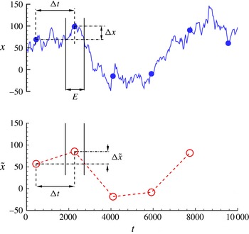
introduces a second time scale that also influences the measured displacement fluctuation and the corresponding interpretation of diffusion coefficient (see illustration in figure 1). In actual particle-tracking experiments, other localization errors connected with the noise and limited spatial resolution of the detector can additionally compromise the accuracy of particle displacement measurement (Thompson, Larson & Webb Reference Thompson, Larson and Webb2002; Montiel, Cang & Yang Reference Montiel, Cang and Yang2006; Berglund Reference Berglund2010; Michalet Reference Michalet2010).
One-dimensional trajectory of a single Brownian particle in time. Solid line: instantaneous trajectory, solid symbol: instantaneous position at time interval
 ${\rm\Delta}t$
, open symbol: averaged position within exposure period
 $E$
. A detector with averaging period
 $E$
would report particle displacement
 ${\rm\Delta}\tilde{x}$
instead of
 ${\rm\Delta}x$
from an instantaneous trajectory.

The issue of finite integration/exposure time becomes especially important as the use of nano-particles of decreasing size becomes more commonplace, e.g. in near-surface measurements with evanescent wave illumination using fluorescent coated particles (Zettner & Yoda Reference Zettner and Yoda2003; Jin et al. Reference Jin, Huang, Park, Yoo and Breuer2004; Sadr et al. Reference Sadr, Yoda, Zheng and Conlisk2004) and quantum-dot (QD) nano-particles (Pouya et al. Reference Pouya, Koochesfahani, Snee, Bawendi and Nocera2005, Reference Pouya, Koochesfahani, Greytak, Bawendi and Nocera2008). Such measurements often require longer detection exposure/integration periods to compensate for the much reduced optical signal of nano-particles. The longer integration period, coupled with the much larger diffusivity of nano-particles, can result in measured displacements that are significantly different from those based on instantaneous positions. The finite exposure/integration time has also been a factor in studies of single-molecule tracking within plasma cells (Ritchie et al. Reference Ritchie, Shan, Kondo, Iwasawa, Fujiwara and Kusumi2005; Destainville & Salomé Reference Destainville and Salomé2006). However, these studies are focused on the particular case of confined diffusion within a cell (rectangular or circular box), which inherently introduces other time scales that complicate isolating the influence of the exposure time by itself. While analysing the source of errors in particle-tracking microrheology, Savin & Doyle (Reference Savin and Doyle2005) studied the contribution of a finite exposure time using theory and experiments and showed a ‘dynamic error’ in mean-squared displacement estimation was introduced from the particle motion during the exposure time and that the error scaled linearly with the exposure time.
The goal of this article is to build on Savin and Doyle’s work on free diffusion and address the influence of the second time scale, imposed by the observation averaging time
 $E$
(or in non-dimensional form
 $E/{\rm\Delta}t$
), on estimation of displacement fluctuation due to Brownian motion when the particle motion is hindered by the presence of a solid wall. In particular, our study addresses the basic solution to Brownian fluctuation and the nature of its mathematical form over the entire range of the control parameter
 $E/{\rm\Delta}t$
(i.e. both smaller and larger than unity). While the motivation behind this study originates from the experimental constraints of finite
 $E$
, and problem definition is informed by typical experimental arrangements, the study here is purely fundamental in nature.
The approach taken here is numerical simulation of Brownian motion based on the Langevin equation. This approach avoids the uncertainties in experiments related to noise and localization errors, thus allowing us to focus on the integration time issue alone. We first consider the simpler case of free diffusion, for which an exact analytical solution already exists over the range
 $E/{\rm\Delta}t\leqslant 1$
(Savin & Doyle Reference Savin and Doyle2005), and confirm complete agreement between simulation results and exact solution. In addition, we present a new derivation for the exact solution that covers both regions of the non-dimensional parameter range (
 $E/{\rm\Delta}t\leqslant 1$
and
 $E/{\rm\Delta}t\geqslant 1$
), which, as we will demonstrate, exhibit two different scaling laws. We then consider the more challenging case of Brownian motion of nano-particles and estimation of the parallel diffusion coefficient near a solid wall where the motion is hindered, with spatially varying diffusion. In this case an exact analytical solution would be difficult to obtain, and to our knowledge does not exist.
2. Brownian simulation
The problem statement can be described with the help of figure 1, illustrating a representative one-dimensional path of an arbitrary particle in space under Brownian motion. The instantaneous trajectory shown on the upper plot is sampled at certain time ticks (solid symbols) separated by time step
 ${\rm\Delta}t$
. The displacement (
 ${\rm\Delta}x$
) measured between these instantaneous locations is distributed normally with a standard deviation of
 $\sqrt{2D{\rm\Delta}t}$
according to the theory of Brownian motion. The averaged positions over time interval
 $E$
recorded by a detector form the trajectory shown in the lower plot of figure 1, with open symbols representing the recorded positions over each exposure/integration time period
 $E$
. It is evident that, in general, the averaged and instantaneous locations do not correspond to one another and therefore the measured displacements (
 ${\rm\Delta}\tilde{x}$
) are different from those representing the actual Brownian motion. We chose to use numerical simulations to study how the parameter
 $E$
(or
 $E/{\rm\Delta}t$
in non-dimensional form) affects the displacement distribution and the corresponding estimated diffusion coefficient.
The Brownian motion of suspended particles has been successfully simulated in a variety of flowing and non-flowing situations with different boundary conditions. Usually, two general approaches, based on Langevin or Fokker–Planck formulations, are used to numerically simulate the motion of a group of particles in the solution (Ermak & Mccammon Reference Ermak and Mccammon1978). With Langevin’s approach the time–space trajectories of individual particles are calculated by integrating the appropriate equation of motion over time, while in the Fokker–Plank description the time evolution of the particle phase-space distribution function is directly obtained by solving the Fokker–Planck differential equation. Here we employ the former method to simulate the motion of individual nano-particles.
The simulation of Brownian motion using Langevin equations has been successfully demonstrated (Adamczyk, Siwek & Szyk Reference Adamczyk, Siwek and Szyk1995; Sholl et al. Reference Sholl, Fenwick, Atman and Prieve2000; Sadr, Li & Yoda Reference Sadr, Li and Yoda2005; Unni & Yang Reference Unni and Yang2005; Huang, Guasto & Breuer Reference Huang, Guasto and Breuer2009). The Langevin equation for a Brownian particle immersed in a fluid medium can be written as (Unni & Yang Reference Unni and Yang2005):
 $$\begin{eqnarray}\text{d}\boldsymbol{r}=\frac{\unicode[STIX]{x1D63F}(t)\boldsymbol{F}(t)}{k_{B}T}{\it\delta}t+\boldsymbol{{\rm\nabla}}\unicode[STIX]{x1D63F}(t){\it\delta}t+\left({\rm\Delta}\boldsymbol{r}\right)^{B},\end{eqnarray}$$
where
 $\text{d}\boldsymbol{r}$
is change in the position vector of the particle,
 $\unicode[STIX]{x1D63F}$
is the diffusivity tensor (accounting for the dependence of the diffusion coefficient on the direction of the motion),
 $\boldsymbol{F}$
is the total external force acting on the particle,
 $({\rm\Delta}\boldsymbol{r})^{B}$
is the random Brownian displacement of the particle,
 ${\it\delta}t$
is the time interval,
 $T$
is the temperature of the fluid and
 $k_{B}$
is the Boltzmann constant. The simulation starts with a group of particles randomly distributed in a predefined spatial domain and then the spatial coordinates of each particle are updated by integrating the equation of motion (2.1) over a small finite time step, while all terms are evaluated at the starting time. Since often a dilute solution of particles is used in particle-tracking measurements, we shall ignore any inter-particle interactions in the simulations presented here. With this assumption and accounting for anisotropic diffusion near surfaces, the diffusivity tensor is reduced to a vector of the form
 $\boldsymbol{D}=D_{\infty }[{\it\beta},{\it\beta},{\it\xi}]$
, where
 $D_{\infty }$
is the diffusion coefficient in free medium based on the Stokes–Einstein equation and
 ${\it\beta}$
and
 ${\it\xi}$
are the hindered diffusion correction factors parallel and normal to the wall, respectively, which can be approximated by (Goldman, Cox & Brenner Reference Goldman, Cox and Brenner1967; Bevan & Prieve Reference Bevan and Prieve2000):
 $$\begin{eqnarray}\displaystyle & \displaystyle {\it\xi}=\frac{6h^{2}+2ah}{3h^{2}+9ah+2a^{2}} & \displaystyle\end{eqnarray}$$
 $$\begin{eqnarray}\displaystyle & \displaystyle {\it\beta}=\left\{\begin{array}{@{}ll@{}}\displaystyle 1-\frac{9}{16}\left(\frac{a}{a+h}\right)+\frac{1}{8}\left(\frac{a}{a+h}\right)^{3}-\frac{45}{256}\left(\frac{a}{a+h}\right)^{4}-\frac{1}{16}\left(\frac{a}{a+h}\right)^{5}\quad & h/a>1\\ \displaystyle \frac{2\left(\ln \displaystyle \left(\frac{h}{a}\right)-0.9543\right)}{\left(\ln \displaystyle \left(\frac{h}{a}\right)\right)^{2}-4.325\ln \displaystyle \left(\frac{h}{a}\right)+1.591}\quad & h/a<1.\end{array}\right. & \displaystyle \nonumber\\ \displaystyle & & \displaystyle\end{eqnarray}$$
 $a$
is the particle radius and
 $h$
is the particle separation distance from the wall (see figure 2). In this study we have ignored the electrostatic and van der Waals forces. The contribution of gravity, though included in the simulation, was negligible due to the small size of the nano-particles. We should mention that, based on preliminary simulations, the results reported here appear to still hold when electrostatic forces, and the resulting non-uniform particle distribution near a surface, are included; see the Conclusions. The last term in (2.1), representing the random Brownian motion, is modelled as a normal distribution
 $N(0,\sqrt{2D{\it\delta}t})$
. For the simple case of pure diffusion in free medium and in the absence of gravity, the right-hand side of (2.1) reduces to this last term only.
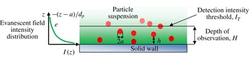
Near-surface imaging with evanescent wave illumination.

The simulation is carried out using the non-dimensional form of (2.1). The particle radius,
 $a$
, and the time to diffuse across this radius,
 ${a^{2}/D}_{\infty }$
, are used as length and time scales of normalization, respectively. A total of
 $10^{5}$
particles are uniformly distributed within a predefined region in space (typically 100
 $a$
–150
 $a$
in all directions). The trajectory of each individual particle is tracked over an infinite domain (
 $-\infty <x,y,z<\infty$
) using (2.1), where all the terms are updated in each time step. Following previous studies (Ermak & Mccammon Reference Ermak and Mccammon1978; Huang et al.
Reference Huang, Guasto and Breuer2009), the (non-dimensional) integration time step
 ${\it\delta}t$
is chosen as
 $10^{-3}$
, which is small enough to ensure numerical accuracy and large enough compared to the particle relaxation time (
 ${\approx}10^{-5}$
), as necessary for validity of the diffusion model. For the near-wall simulations, due to the discrete and finite nature of the computational process, a particle may attempt to enter the solid wall during the integration time step even with a short time step (despite the fact that with the assumption of a no-slip boundary condition, the diffusion coefficient vanishes and particles come to rest at the surface of the solid). To avoid such events, we use a simple specular reflection on the solid wall (i.e. the momentum component normal to the wall changes sign). Since the number of such occurrences is very small (
 $10^{-5}\,\%{-}10^{-3}\,\%$
of total events calculated), the specular reflection assumption does not affect the final statistical parameters computed from the simulation. In near-wall simulations particle trajectories are tracked over an infinite domain in
 $x,y$
and a semi-infinite domain in
 $z$
, i.e.
 $a\leqslant z<\infty$
.
The outcome of the simulation is the trajectory
 $x(t)$
of each particle calculated with the fine resolution
 ${\it\delta}t$
. The effect of detector finite exposure/integration period is modelled by simply integrating the path of individual particles during the predefined exposure time
 $E$
, i.e.:
 $$\begin{eqnarray}\tilde{x}\left(t_{k}\right)=\frac{1}{E}\int _{t_{k}}^{t_{k}+E}x(t)\text{d}t,\end{eqnarray}$$
where
 $\tilde{x}$
is the average position of the particle within the exposure time
 $E$
at time tick
 $t_{k}$
, while
 $x$
is the instantaneous position. We note that in particle-tracking experiments,
 $\tilde{x}$
is usually inferred from the average intensity distribution of the particle image on the detector, typically through a best-fit over its intensity distribution. The influence of such approaches has been considered under particle localization errors (e.g. see references cited in the Introduction) and is outside the scope of the current study. The simulation is typically carried out for
 $10^{7}$
time steps and the particle displacements
 ${\rm\Delta}\tilde{x}$
over the prescribed time period
 ${\rm\Delta}t$
are used to estimate the diffusion coefficient
 $\tilde{D}$
according to
 $\tilde{D}=\langle ({\rm\Delta}\tilde{x})^{2}\rangle /2{\rm\Delta}t$
, where
 $\langle ({\rm\Delta}\tilde{x})^{2}\rangle$
represents the expected value of mean square displacement. For the case of free diffusion, the diffusion vector in (2.1) is a constant; therefore displacements from all the particles within the simulation can be used to evaluate this diffusion coefficient.
For near-wall simulations, however, diffusion is a function of particle distance from the wall. The estimated diffusion coefficient depends, therefore, on the extent of the domain normal to the wall used to evaluate this coefficient. In order to specify this domain size
 $H$
, we use an approach that is borrowed from experiments. In experimental near-wall measurements based on evanescent wave illumination, the extent of the observed domain
 $H$
is determined by the thickness of the illumination region (i.e. the evanescent layer thickness), camera detection capability and the intensity threshold used in the image processing to identify the particles (figure 2). To include a similar processing in the simulation data, an equivalent brightness (intensity value) is assigned to each particle in the Langevin simulation, depending on the particle distance from the wall at each instant of time. In near-wall measurements using total internal reflection microscopy, the distance-dependent intensity is given by the exponential intensity distribution of the evanescent field, i.e.:
 $$\begin{eqnarray}I(z)=\text{e}^{-(z-a/d_{p})},\end{eqnarray}$$
where
 $I(z)$
is the normalized intensity of the particle located at distance
 $z$
from the wall relative to a reference value (chosen to be the intensity of a particle in contact with the wall) and
 $d_{p}$
is the penetration depth of the evanescent field. In the simulations
 $d_{p}/a$
is set to 13, consistent with previous near-wall QD imaging experiments (
 $d_{p}\approx 100~\text{nm},a\approx 8~\text{nm}$
) (Pouya et al.
Reference Pouya, Koochesfahani, Greytak, Bawendi and Nocera2008). Other values of
 $d_{p}/a$
can be considered easily, if needed, by interrogating the results for different values of intensity threshold, as described next.
In near-wall simulations, the intensity value is calculated for all the particles in each time step of the simulation. A detector with integration/exposure time
 $E$
would report the average intensity of the particle over the portion of its trajectory in each exposure, i.e. for a given particle the average intensity at time
 $t_{k}$
is:
 $$\begin{eqnarray}\tilde{I} \left(t_{k}\right)=\frac{1}{E}\int _{t_{k}}^{t_{k}+E}I(z(t))\text{d}t.\end{eqnarray}$$
Particles are considered ‘detectable’ if their average intensity
 $\tilde{I}$
(over integration period
 $E$
) is above a prescribed intensity threshold
 $I_{T}$
. Therefore, in near-wall simulations only particles that are detectable at the beginning and end of the interrogation time interval
 ${\rm\Delta}t$
are kept in the data ensemble for further processing, and their corresponding particle displacements
 ${\rm\Delta}\tilde{x}$
are used to estimate the diffusion coefficient
 $\tilde{D}$
. We note that the prescribed intensity threshold
 $I_{T}$
essentially sets the size of the near-wall domain
 $H$
that gets used in the estimation of diffusion coefficient. The relation between
 $I_{T}$
and
 $H$
is direct and unambiguous only in the limit of
 $E\rightarrow 0$
, given by
 $H/a=1-(d_{p}/a)\ln (I_{T})$
, according to (2.4). When
 $E\neq 0$
, the direct relation between the measured particle intensity and its location within the evanescent layer is lost, e.g. the position corresponding to a particle with average intensity
 $\tilde{I} \geqslant I_{T}$
(i.e. a detectable particle) may be beyond the distance
 $H$
, depending on the extent of the Brownian fluctuation.
3. Results and discussion
3.1. Free diffusion
We first focus on the case of free diffusion (with prescribed diffusion coefficient
 $D_{\infty }$
) to single out the effect of the exposure/integration time period
 $E$
. The diffusion coefficients
 $\tilde{D}$
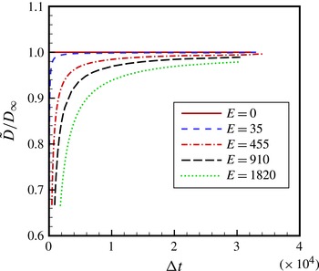
estimated from the computed mean square displacement of particle displacements are illustrated in figure 3 over a broad range of interrogation time intervals
 ${\rm\Delta}t$
and selected values of integration periods
 $E\leqslant {\rm\Delta}t$
. We note that in the case of
 $E=0$
the estimated diffusion coefficient from simulations recovers the prescribed
 $D_{\infty }$
and is independent of the interrogation time interval
 ${\rm\Delta}t$
, as expected. However, for any non-zero value of sampling/interrogation period the estimated diffusion coefficient
 $\tilde{D}$
becomes dependent on
 ${\rm\Delta}t$
, starting with low estimated values at small
 ${\rm\Delta}t$
and asymptotically approaching the correct particle diffusion coefficient
 $D_{\infty }$
at large values of
 ${\rm\Delta}t$
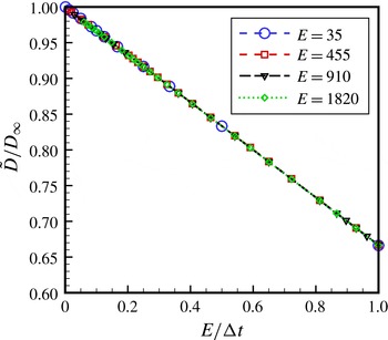
. The scaling behaviour of the data becomes apparent once the curves in figure 3 are rescaled in terms of
 $E/{\rm\Delta}t$
, as depicted in figure 4. We can see that all the simulation data for
 $0\leqslant E/{\rm\Delta}t\leqslant 1$
collapse onto a single curve showing a linearly decreasing
 $\tilde{D}/D_{\infty }$
versus
 $E/{\rm\Delta}t$
with a
 $-1/3$
slope. The lowest value of the estimated diffusion coefficient would be
 $\tilde{D}/D_{\infty }=2/3$
, which occurs at
 $E/{\rm\Delta}t=1$
(this would be the case when the camera image frame rate sets the interrogation time interval
 ${\rm\Delta}t$
and the camera shutter is fully open).
Estimated diffusion coefficient versus time delay at various exposure times for free diffusion over the range
 $E/{\rm\Delta}t\leqslant 1$
.

Estimated diffusion coefficient versus
 $E/{\rm\Delta}t$
for free diffusion over the range
 $E/{\rm\Delta}t\leqslant 1$
. Only selected points from figure 3 are shown to reduce clutter. The data collapse onto a line with slope
 $-1/3$
.

We now present a theoretical approach to obtain a closed-form solution for the scaling behaviour revealed by the simulations. The approach relies on methods of stochastic differential equations (Øksendal Reference Øksendal1998) and details of the steps are given in appendix A. We consider Brownian motion
 $B_{t}({\it\omega})$
for particle
 ${\it\omega}$
in time
 $t$
, such that it is a continuous function and follows a Gaussian process with an arbitrarily selected mean of zero and a standard deviation of
 $t$
. The process also has independent increments, i.e. for
 $0\leqslant t_{1}\leqslant \cdots \leqslant t_{k}$
,
 $B_{t_{1}},B_{t_{2}}-B_{t_{1}},\dots ,B_{t_{k}}-B_{t_{k-1}}$
are independent. In this description,
 $B_{t}$
is connected to the position of the Brownian particle with a diffusion coefficient of
 $D_{\infty }$
according to:
 $$\begin{eqnarray}x_{t}=\sqrt{2D_{\infty }}B_{t}.\end{eqnarray}$$
We sample the Brownian motion (in experiment or simulation) at time ticks
 $t_{k}=k{\rm\Delta}t$
and at each time tick the mean position is calculated over the interval
 $(t_{k},t_{k}+E)$
with the integration/exposure period
 $E$
in the range
 $0\leqslant E\leqslant {\rm\Delta}t$
, i.e.:
 $$\begin{eqnarray}\tilde{x}_{t_{k}}=\frac{1}{E}\int _{t_{k}}^{t_{k}+E}x_{t}\text{d}t.\end{eqnarray}$$
Then we estimate the diffusion coefficient with:
 $$\begin{eqnarray}\tilde{D}=\frac{\langle \left(\tilde{x}_{t_{k+1}}-\tilde{x}_{t_{k}}\right)^{2}\rangle }{2{\rm\Delta}t}=\frac{1}{2{\rm\Delta}t}\langle \tilde{x}_{k+1}^{2}-2\tilde{x}_{t_{k+1}}\tilde{x}_{t_{k}}+\tilde{x}_{t_{k}}^{2}\rangle ,\end{eqnarray}$$
where the symbol
 $\langle \,\rangle$
stands for the expected value. By iterated integration and independent increments we know that (see appendix A):
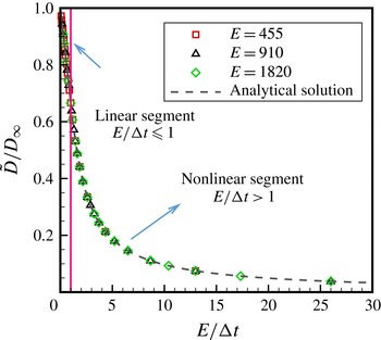
Estimated diffusion coefficient for free diffusion over the range
 $E/{\rm\Delta}t>1$
. The lower range is also shown for completion. The analytical solution is given by (3.5).

 $\langle \tilde{x}_{t_{k}}\tilde{x}_{t_{k+1}}\rangle =2D_{\infty }(t_{k}+E/2)$
and
 $\langle \tilde{x}_{t_{k}}^{2}\rangle =2D_{\infty }(t_{k}+E/3)$
. Therefore, the estimated diffusion coefficient from (3.3) reduces to
 $$\begin{eqnarray}\frac{\tilde{D}}{D_{\infty }}=1-\frac{1}{3}\left(\frac{E}{{\rm\Delta}t}\right)\quad \text{for }0\leqslant E/{\rm\Delta}t\leqslant 1.\end{eqnarray}$$
This closed-form exact solution provides the fundamental foundation for the scaling result described earlier on the basis of the simulation data. We note that Savin & Doyle (Reference Savin and Doyle2005) obtained the same solution while analysing the source of errors in particle-tracking microrheology. Their solution method considered the averaging process in the spatial frequency domain and took advantage of Fourier transform techniques. The new derivation method we have presented will allow us to also extend the analysis to the parameter range
 $E/{\rm\Delta}t>1$
, as described next.
We have so far focused the discussion on the parameter range
 $E/{\rm\Delta}t\leqslant 1$
, as motivated by a typical imaging system where the maximum exposure (fully open shutter) is limited by the inter-frame time, hence
 $E/{\rm\Delta}t=1$
. We now consider the case when the integration/exposure time
 $E$
is greater than the interrogation time interval
 ${\rm\Delta}t,~E/{\rm\Delta}t>1$
. Experimentally, this would be achieved by using two independent detectors that record images with a time delay
 ${\rm\Delta}t$
relative to each other. Although this may not represent a typical imaging configuration, the mathematical nature of the solution over this parameter range is nevertheless an interesting question.
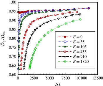
Apparent diffusion coefficient of particles near a solid wall over the range
 $E/{\rm\Delta}t\leqslant 1$
. Intensity threshold
 $I_{T}=0.05$
(equivalent to
 $H=40a,~H\cong 3d_{p}$
for
 $E=0$
).

The estimated diffusion coefficients from the simulations for multiple
 $E$
and
 ${\rm\Delta}t$
values, with
 $E>{\rm\Delta}t$
, are illustrated in figure 5 versus
 $E/{\rm\Delta}t$
. Interestingly, the normalized data over the range
 $E/{\rm\Delta}t>1$
also collapse onto a single curve, which is now nonlinear, in contrast to the linear scaling law over the range
 $E/{\rm\Delta}t\leqslant 1$
. This collapse of the simulation data prompted us to seek the exact solution for the functional form of the solution using the theoretical approach presented earlier. In re-evaluating (3.3), we note that the term
 $\langle \tilde{x}_{t_{k}}^{2}\rangle$
remains unchanged and, according to details given in appendix A,
 $\langle \tilde{x}_{t_{k}}\tilde{x}_{t_{k+1}}\rangle =D_{\infty }(t_{k}+{\rm\Delta}t/2-({\rm\Delta}t^{2}/E)/2+({\rm\Delta}t^{3}/E^{2})/6+E/3)$
, arriving at the final result:
 $$\begin{eqnarray}\frac{\tilde{D}}{D_{\infty }}=\left(\frac{E}{{\rm\Delta}t}\right)^{-1}-\frac{1}{3}\left(\frac{E}{{\rm\Delta}t}\right)^{-2}=\left(\frac{E}{{\rm\Delta}t}\right)^{-1}\left[1-\frac{1}{3}\left(\frac{E}{{\rm\Delta}t}\right)^{-1}\right]\quad \text{for }E/{\rm\Delta}t>1.\end{eqnarray}$$
This exact solution is added to figure 5 and perfectly complements the simulation data.
3.2. Near-wall hindered diffusion
We now return to the simulation of (2.1) for the case of diffusion of particles near a solid wall. The particles are initially distributed uniformly in the near-wall region over the extent of
 $1<z/a<150$
. This region, being more than ten times larger than the evanescent layer thickness, is large enough to ensure the particle distribution remains uniform over the simulation time frame within the near-wall sub-region used in calculating particle displacement statistics (a uniform distribution is expected due to absence of electrostatic interactions in the simulations). We first illustrate the general nature of the results for the intensity threshold value of
 $I_{T}=0.05$
(corresponding to near-wall domain size
 $H=40a$
, or
 $H\cong 3d_{p}$
, in the limit of zero exposure), i.e. only particles whose average intensity is less than this value are used in the data analysis. This value of intensity threshold is chosen based on the typical values used in previous experiments (Pouya et al.
Reference Pouya, Koochesfahani, Snee, Bawendi and Nocera2005, Reference Pouya, Koochesfahani, Greytak, Bawendi and Nocera2008). Results for other values of intensity threshold will follow. For the purpose of this article, we focus on diffusion of particles parallel to the wall and particle displacements are calculated using only the in-plane components of the particle 3D trajectories.
Figure 6 shows the apparent in-plane diffusion coefficient
 $\tilde{D}_{\Vert }$
estimated from simulations for multiple integration/exposure values versus the time delay
 ${\rm\Delta}t$
, with
 $E\leqslant {\rm\Delta}t$
. A trend similar to that observed in figure 3 for free diffusion is also evident here, i.e. for any non-zero exposure
 $E$
the estimated diffusion coefficient
 $\tilde{D}_{\Vert }$
strongly depends on
 ${\rm\Delta}t$
, starting with a low value at small
 ${\rm\Delta}t$
and asymptotically approaching the corresponding value
 $D_{\Vert 0}$
for
 $E=0$
at large
 ${\rm\Delta}t$
. There is, however, a fundamental difference in these near-wall results in two respects. First, we note that the value
 $D_{\Vert 0}$
in the limit of zero exposure is less than the free-diffusion coefficient
 $D_{\infty }$
far away from the wall. Since
 $D_{\Vert 0}$
represents the spatially averaged diffusion coefficient of particles within the observed region near the wall (in this case, over domain size
 $H=40a$
, or
 $H\cong 3d_{p}$
), this result is expected due to near-wall hindered diffusion. Second and more importantly, however, the estimated diffusion
 $D_{\Vert 0}$
at zero integration/exposure (
 $E=0$
) shown in figure 6 is no longer a constant and independent of the interrogation time interval
 ${\rm\Delta}t$
, as in free diffusion; the apparent diffusion coefficient gradually increases as
 ${\rm\Delta}t$
increases. This dependence on
 ${\rm\Delta}t$
becomes even more significant for higher intensity thresholds (smaller
 $H$
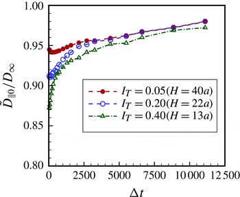
values), as shown in figure 7.
Apparent diffusion coefficient of particles near a solid wall for exposure
 $E=0$
and multiple intensity thresholds. Near-wall domain size
 $H$
is indicated for each intensity threshold.

This behaviour can be qualitatively explained in terms of the asymmetric diffusion of particles near the wall. During the interrogation time interval
 ${\rm\Delta}t$
, even though particles are free to diffuse in and out of the predefined observation domain
 $H$
, near a solid wall particles are more likely to diffuse away from the wall than towards the wall due to near-wall hindered diffusion. As a result, a particle is more likely to ‘sample’ regions farther away from the wall (with a higher diffusion coefficient approaching free diffusion
 $D_{\infty }$
) than closer to the wall (with a smaller diffusion coefficient approaching zero), leading to an ‘apparent’ diffusion that is biased towards
 $D_{\infty }$
. With increasing time interval
 ${\rm\Delta}t$
, this asymmetric behaviour becomes increasingly more pronounced, which drives the bias in the observed ‘average’ diffusion coefficient increasingly towards
 $D_{\infty }$
. The effect also becomes more pronounced as the domain size (
 $H$
) shrinks. The diffusion-induced bias just described for the near-wall diffusion coefficient has also been observed in near-wall velocimetry studies, where the asymmetric diffusion leads to a larger apparent mean velocity that increases with delay time (Sadr et al.
Reference Sadr, Hohenegger, Li, Mucha and Yoda2007; Pouya et al.
Reference Pouya, Koochesfahani, Greytak, Bawendi and Nocera2008; Huang et al.
Reference Huang, Guasto and Breuer2009).
When considering the scaling behaviour of the near-wall diffusion estimates
 $\tilde{D}_{\Vert }$
in figure 6 for non-zero integration/exposure
 $E$
, we observe that the physical process that leads to the bias described above in the limiting value of the estimated diffusion
 $D_{\Vert 0}$
at
 $E=0$
, and therefore its dependence on
 ${\rm\Delta}t$
, would also occur regardless of the finite exposure time
 $E\neq 0$
. The correct normalization of apparent diffusion coefficient
 $\tilde{D}_{\Vert }$
should account for this bias and, therefore, using
 $D_{\Vert 0}$
for scaling is expected to be more appropriate than
 $D_{\infty }$
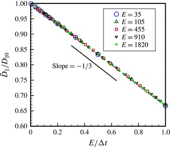
. Once the data in figure 6 for intensity threshold
 $I_{T}=0.05$
are rescaled in terms of
 $\tilde{D}_{\Vert }/D_{\Vert 0}$
and plotted versus
 $E/{\rm\Delta}t$
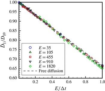
, see figure 8, the data do in fact collapse onto a single curve, apparently following the same linear scaling law as in free diffusion, with a
 $-1/3$
slope. Upon closer examination, however, we find that the simulation data in figure 8 deviate ever so slightly from the
 $-1/3$
slope. The deviation becomes more apparent at higher intensity thresholds (i.e. smaller near-wall domain size
 $H$
). This is illustrated in figure 9 for the case of
 $I_{T}=0.4$
, where the departure from the
 $-1/3$
slope becomes more and more evident with increasing values of
 $E$
.
Apparent diffusion coefficient normalized with the diffusion coefficient at zero exposure for near-wall hindered diffusion over the range
 $E/{\rm\Delta}t\leqslant 1$
. Intensity threshold
 $I_{T}=0.05$
.

Apparent diffusion coefficient normalized with the diffusion coefficient at zero exposure for near-wall hindered diffusion over the range
 $E/{\rm\Delta}t\leqslant 1$
. Intensity threshold
 $I_{T}=0.4$
. The dashed line corresponding to free diffusion has a slope of
 $-1/3$
.

The theoretical underpinning behind the results just described does not exist; in the case of diffusion near a solid wall where the motion is hindered, with spatially varying diffusion, it would be difficult to obtain an exact analytical solution, and to our knowledge it does not exist. However, our results show that the form of the scaling law obtained for free diffusion applies with a high degree of accuracy to the parallel diffusion coefficient for near-wall hindered diffusion. In particular, the normalized parallel diffusion coefficient can be written as a slightly modified form of the free-diffusion scaling law (equation (3.4)) by adjusting the
 $-1/3$
linear slope by a small fraction
 ${\it\epsilon}$
, as indicated below:
 $$\begin{eqnarray}\frac{\tilde{D}_{\Vert }}{D_{\Vert 0}}=1-\frac{1}{3}(1+{\it\epsilon})\left(\frac{E}{{\rm\Delta}t}\right)\quad \text{for }0\leqslant E/{\rm\Delta}t\leqslant 1.\end{eqnarray}$$
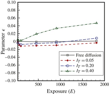
Figure 10 summarizes the values of
 ${\it\epsilon}$
for multiple intensity thresholds versus integration/exposure time
 $E$
over the range
 $E/{\rm\Delta}t\leqslant 1$
. In each case,
 ${\it\epsilon}$
was arrived at from the least-squares fit of
 $\tilde{D}_{\Vert }/D_{\Vert 0}$
versus
 $E/{\rm\Delta}t$
simulation data (e.g. figures 8, 9) to (3.6). The resulting fit to data was excellent, with the average deviation between simulation data and (3.6) varying between zero and approximately 0.005 over the entire range of
 $E$
values shown in figure 10. It is noted from this figure that the values of
 ${\it\epsilon}$
are indeed small. For studies in the literature to date, values of
 $E$
are limited to
 $E<600$
, corresponding to
 ${\it\epsilon}<0.03$
in figure 10.
The deviation of hindered diffusion scaling law from free diffusion (parameter
 ${\it\epsilon}$
in (3.6)) for several values of intensity threshold over the range
 $E/{\rm\Delta}t\leqslant 1$
. For studies in the literature to date,
 $E<600$
.

The near-wall diffusion results discussed above over the parameter range
 $E/{\rm\Delta}t\leqslant 1$
are extended next to
 $E/{\rm\Delta}t>1$
by considering the apparent in-plane diffusion coefficient
 $\tilde{D}_{\Vert }$
estimated from near-wall simulations for multiple
 $E$
and
 ${\rm\Delta}t$
values, with
 $E>{\rm\Delta}t$
, and different values of intensity threshold
 $I_{T}$
. Results for
 $I_{T}=0.05$
are given in figure 11 in terms of
 $\tilde{D}_{\Vert }/D_{\Vert 0}$
versus
 $E/{\rm\Delta}t$
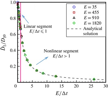
. Interestingly, the normalized data over the range
 $E/{\rm\Delta}t>1$
also collapse onto a single curve, a nonlinear curve whose functional form appears to be the same as that for the case of free diffusion (see figure 5 and (3.5)). Similar to the case of
 $E/{\rm\Delta}t\leqslant 1$
, we find upon close inspection that there is a small deviation between the simulation results in figure 11 and the free-diffusion theory given by (3.5), and that the deviation becomes more noticeable at higher intensity thresholds, though still small.
Normalized diffusion coefficient for near-wall hindered diffusion over the range
 $E/{\rm\Delta}t>1$
for intensity threshold
 $I_{T}=0.05$
. The lower range is also shown for completion. The analytical solution is given by (3.7).

In the absence of an exact theoretical solution, we consider the same approach as that demonstrated earlier in the case of
 $E/{\rm\Delta}t\leqslant 1$
and find that the form of the scaling law obtained for free diffusion over
 $E/{\rm\Delta}t>1$
applies with a high degree of accuracy to the parallel diffusion coefficient for near-wall hindered diffusion as well. In particular, the normalized parallel diffusion coefficient can be written as a slightly modified form of the free-diffusion scaling law for
 $E/{\rm\Delta}t>1$
(i.e. (3.5)) by adjusting the
 $-1/3$
constant by a small fraction
 ${\it\epsilon}$
, as indicated below:
 $$\begin{eqnarray}\frac{\tilde{D}_{\Vert }}{D_{\Vert 0}}=\left(\frac{E}{{\rm\Delta}t}\right)^{-1}\left[1-\frac{1}{3}(1+{\it\epsilon})\left(\frac{E}{{\rm\Delta}t}\right)^{-1}\right]\quad \text{for }E/{\rm\Delta}t>1.\end{eqnarray}$$
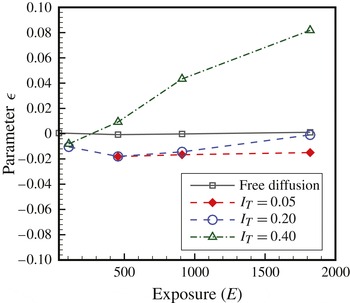
Corresponding values of
 ${\it\epsilon}$
are plotted in figure 12 versus integration/exposure time
 $E$
over the range
 $E/{\rm\Delta}t>1$
for different intensity thresholds, where the
 ${\it\epsilon}$
values were obtained from the least-squares fit of
 $\tilde{D}_{\Vert }/D_{\Vert 0}$
versus
 $E/{\rm\Delta}t$
simulation data to (3.7). As in the case of
 $E/{\rm\Delta}t\leqslant 1$
, the resulting fit to data was again excellent, with the average deviation between simulation data and (3.7) varying between zero and approximately 0.005 over the entire range of
 $E$
values shown in figure 12. One can note that, although the trends for
 ${\it\epsilon}$
in
 $E/{\rm\Delta}t>1$
are similar to those of
 $E/{\rm\Delta}t\leqslant 1$
, the actual values are different and tend to be slightly larger for
 $E/{\rm\Delta}t>1$
. Nevertheless, values of
 ${\it\epsilon}$
are still small for a wide range of parameters and for the studies reported in the literature to date (i.e.
 $E<600$
) we expect
 ${\it\epsilon}<0.03$
, based on figure 11.
The deviation of hindered diffusion scaling law from free diffusion (parameter
 ${\it\epsilon}$
in (3.7)) for several values of intensity threshold over the range
 $E/{\rm\Delta}t>1$
. For studies in the literature to date,
 $E<600$
.

4. Concluding remarks
Numerical simulation of Brownian diffusion of small particles was carried out to determine the influence of finite sampling time
 $E$
, relative to interrogation time interval
 ${\rm\Delta}t$
, on the estimation of diffusion coefficient for both free diffusion and near-wall hindered diffusion. Results of free-diffusion simulations recovered the known linear scaling law, found by Savin & Doyle (Reference Savin and Doyle2005), for dependency of the estimated diffusion coefficient
 $\tilde{D}$
on
 $E/{\rm\Delta}t$
over the range
 $0\leqslant E/{\rm\Delta}t\leqslant 1$
, given by
 $\tilde{D}/D_{\infty }=1-(1/3)(E/{\rm\Delta}t)$
. Results were extended to the parameter range
 $E/{\rm\Delta}t>1$
, where we found data collapse onto a new nonlinear scaling law, whose functional form was shown to have the exact analytical solution given by
 $$\begin{eqnarray}\frac{\tilde{D}}{D_{\infty }}=\left(\frac{E}{{\rm\Delta}t}\right)^{-1}\left[1-\frac{1}{3}\left(\frac{E}{{\rm\Delta}t}\right)^{-1}\right].\end{eqnarray}$$
Simulations of near-wall hindered diffusion revealed the interesting result that the estimated in-plane diffusion coefficient
 $\tilde{D}_{\Vert }$
, when normalized by the corresponding value
 $D_{\Vert 0}$
in the limit of
 $E=0$
, could be accurately represented by the same form of scaling laws described above for free diffusion, but with a small modification. The modification involved replacing the
 $-1/3$
constant in the free-diffusion scaling laws, for regions
 $0\leqslant E/{\rm\Delta}t\leqslant 1$
and
 $E/{\rm\Delta}t>1$
, by
 $-(1+{\it\epsilon})/3$
, where the small parameter
 ${\it\epsilon}$
depends on the size of the near-wall domain used in the estimation of the diffusion coefficient and the value of
 $E$
. For the range of parameters reported in the literature, we estimate
 ${\it\epsilon}<0.03$
.
Our near-wall simulations also showed that even in the limit of
 $E=0$
there was a bias in the estimated near-wall diffusion coefficient parallel to the wall,
 $D_{\Vert 0}$
, due to asymmetric diffusion next to an impermeable wall. The estimated diffusion coefficient in this case was found to be a function of interrogation time interval
 ${\rm\Delta}t$
, where the diffusion coefficient was increasingly overestimated as
 ${\rm\Delta}t$
increased. This diffusion-induced effect is similar to the mean velocity overestimation of particles in near-wall measurements, reported analytically by Sadr et al. (Reference Sadr, Hohenegger, Li, Mucha and Yoda2007) and experimentally by Pouya et al. (Reference Pouya, Koochesfahani, Greytak, Bawendi and Nocera2008) and Huang et al. (Reference Huang, Guasto and Breuer2009).
The simulation of hindered diffusion presented here could be expanded by considering other forces that were neglected in this work, such as electrostatic and van der Waals forces that lead to a non-uniform distribution of particles near a charged surface. We have performed preliminary studies while including electrostatic forces and found that the resulting non-uniform particle distribution near the wall (i.e. the Boltzmann distribution) did not appear to change the scaling laws presented in this work. In particular, simulations with a 40 nm Debye layer thickness led to plots very similar to figures 8 and 11, with values
 ${\it\epsilon}$
less than approximately 0.05. More extensive studies are needed to corroborate these preliminary observations. It is noted that addition of non-stochastic external forces (i.e. electrostatic and van der Waals) would not be expected to alter the general form of the scaling laws obtained here for the solution of the Langevin equation, a representation of the Ornstein–Uhlenbeck process (Da Prato & Zabczyk Reference Da Prato and Zabczyk1996).
The closed-form solutions presented here provide the tools needed to assess the influence of experimental parameters (i.e.
 $E$
and
 ${\rm\Delta}t$
) in optical particle tracking on the estimation of the diffusion coefficient. Furthermore, these findings can be used to remove the artefacts caused by finite detector exposure and extrapolate the experimental data to the limit of zero exposure. In doing so, one must also be cognizant of other experimental factors that can additionally compromise the accuracy of particle displacement measurement. These factors, which include particle localization errors due to low image signal-to-noise ratio and finite spatial resolution of the image detector, have been studied previously (Thompson et al.
Reference Thompson, Larson and Webb2002; Montiel et al.
Reference Montiel, Cang and Yang2006; Berglund Reference Berglund2010; Michalet Reference Michalet2010). In most near-wall experimental studies to date, larger nano-particles have been used and the range of exposure and time delays chosen are such that the expected reduction of diffusion coefficient due to finite exposure is buried within the experimental uncertainties that arise from other sources. For example,
 $E/{\rm\Delta}t$
is typically less than 0.2 for most reported results and the expected reduction in diffusion coefficient is approximately 7 %, while measurement uncertainties are often approximately 10 % or higher. Experimental capabilities need to improve in order to resolve the effects reported here. The experiments with smaller nano-particles, where higher exposures are used, have mostly focused on velocimetry so far and do not report the estimated particle diffusion data.
Acknowledgements
This work was supported by the CRC Program of the National Science Foundation, grant numbers CHE-0209898 and CHE-0714028, and partial support by NSF grant numbers NSF-0845061 and NSF-0968360. We wish to also acknowledge the support of the Michigan State University High Performance Computing Center and the Institute for Cyber-Enabled Research. We thank one of the reviewers for pointing out the connection of the Langevin equation to the Ornstein–Uhlenbeck process.
Appendix A
The approach described here relies on methods of stochastic differential equations (see Øksendal Reference Øksendal1998, §2.2 for details) and we use the nomenclature therein. We consider Brownian motion
 $B_{t}({\it\omega})$
for particle
 ${\it\omega}$
at time
 $t$
, where
 $B_{t}$
is connected to the one-dimensional position of the Brownian particle by
 $x_{t}=\sqrt{2D_{\infty }}B_{t}$
. (A scale factor of
 $\sqrt{2D_{\infty }}$
is needed to recover the prescribed diffusion coefficient
 $D_{\infty }$
.) The initial position of the particle
 $x_{0}=\sqrt{2D_{\infty }}B_{0}$
at
 $t=0$
is arbitrarily set at the origin, i.e.
 $x_{0}=B_{0}=0$
, without any loss of generality. In Brownian motion the statistics of particle instantaneous position in time
 $x_{t}$
follows a normal distribution (Øksendal Reference Øksendal1998), in much the same way as the more familiar statistics of particle displacement
 ${\rm\Delta}x$
over time step
 ${\rm\Delta}t$
. The Brownian motion then has the following properties:
-
(i)
 $B_{t}({\it\omega})\sim N(0,t)$
(
$\langle B_{t}\rangle =0,\langle B_{t}^{2}\rangle =t$
, where
$\langle ~\rangle$
stands for the expectation of the parameter inside. Note in general
$\langle B_{t}\rangle =B_{0}$
, but is set to zero without loss of generality)
-
(ii)
$B_{t}$
has independent increments, i.e. for
$0\leqslant t_{1}\leqslant \cdots \leqslant t_{k};~B_{t_{1}},B_{t_{2}}-B_{t_{1}},\dots ,B_{t_{k}}-B_{t_{k-1}}$
are independent.





Then for one-dimensional motion:
 $$\begin{eqnarray}\displaystyle \langle B_{s}B_{t}\rangle & = & \displaystyle \langle B_{s}(B_{s}+B_{t}-B_{s})\rangle \quad \text{assuming }s<t\end{eqnarray}$$
 $$\begin{eqnarray}\displaystyle & = & \displaystyle \langle B_{s}^{2}\rangle +\langle B_{s}(B_{t}-B_{s})\rangle\end{eqnarray}$$
 $$\begin{eqnarray}\displaystyle & = & \displaystyle \langle B_{s}^{2}\rangle +\langle B_{s}\rangle \,\langle B_{t}-B_{s}\rangle\end{eqnarray}$$
 $$\begin{eqnarray}\displaystyle & = & \displaystyle s+0=s.\end{eqnarray}$$
 $\langle B_{s}^{2}\rangle =s$
) and property 2 (independence of
 $B_{s}$
and
 $B_{t}-B_{s}$
). Therefore,
 $$\begin{eqnarray}\langle B_{s}B_{t}\rangle =\min \left(s,t\right)\equiv s\wedge t.\end{eqnarray}$$
The Brownian motion is sampled (in experiment or simulation) at time ticks
 $t_{k}=k{\rm\Delta}t$
, and at each time interval
 $(t_{k},t_{k+1})$
the mean positions are calculated over the intervals of
 $(t_{k},t_{k}+E)$
and
 $(t_{k+1},t_{k+1}+E)$
with integration/exposure
 $0\leqslant E\leqslant {\rm\Delta}t$
:
 $$\begin{eqnarray}\tilde{x}_{t_{k}}=\frac{1}{E}\int _{t_{k}}^{t_{k}+E}x_{t}(t)\text{d}t.\end{eqnarray}$$
Then we estimate the diffusion coefficient with:
 $$\begin{eqnarray}\tilde{D}=\frac{\langle \left(\tilde{x}_{t_{k+1}}-\tilde{x}_{t_{k}}\right)^{2}\rangle }{2{\rm\Delta}t}=\frac{1}{2{\rm\Delta}t}\langle \tilde{x}_{k+1}^{2}-2\tilde{x}_{t_{k+1}}\tilde{x}_{t_{k}}+\tilde{x}_{t_{k}}^{2}\rangle .\end{eqnarray}$$
By iterated integration and independent increments we know that:
 $$\begin{eqnarray}\displaystyle \langle \tilde{x}_{t_{k}}\tilde{x}_{t_{k+1}}\rangle & = & \displaystyle \frac{1}{E^{2}}\int _{t_{k}}^{t_{k}+E}\text{d}s\int _{t_{k+1}}^{t_{k+1}+E}\text{d}t\langle x_{s}x_{t}\rangle\end{eqnarray}$$
 $$\begin{eqnarray}\displaystyle & = & \displaystyle \frac{2D_{\infty }}{E^{2}}\int _{t_{k}}^{t_{k}+E}\text{d}s\int _{t_{k+1}}^{t_{k+1}+E}\text{d}t\langle B_{s}B_{t}\rangle \quad \text{note: use (A2)}\end{eqnarray}$$
 $$\begin{eqnarray}\displaystyle & = & \displaystyle \frac{2D_{\infty }}{E^{2}}\int _{t_{k}}^{t_{k}+E}\text{d}s\int _{t_{k+1}}^{t_{k+1}+E}s\text{d}t\end{eqnarray}$$
 $$\begin{eqnarray}\displaystyle & & \displaystyle (\text{note: }s\in (t_{k},t_{k}+E)<t\in (t_{k+1},t_{k+1}+E))\nonumber\\ \displaystyle & = & \displaystyle \frac{2D_{\infty }}{E^{2}}\int _{t_{k}}^{t_{k}+E}sE\text{d}s=\frac{D_{\infty }}{E}\left(2t_{k}E+E^{2}\right)\nonumber\\ \displaystyle & = & \displaystyle 2D_{\infty }t_{k}+D_{\infty }E=2D_{\infty }\left(t_{k}-\frac{E}{2}\right).\end{eqnarray}$$
 $$\begin{eqnarray}\displaystyle \langle \tilde{x}_{t_{k}}^{2}\rangle & = & \displaystyle \frac{1}{E^{2}}\int _{t_{k}}^{t_{k}+E}\text{d}s\int _{t_{k}}^{t_{k}+E}\text{d}t\langle x_{s}x_{t}\rangle\end{eqnarray}$$
 $$\begin{eqnarray}\displaystyle & = & \displaystyle \frac{2D_{\infty }}{E^{2}}\int _{t_{k}}^{t_{k}+E}\text{d}s\int _{t_{k}}^{t_{k}+E}\text{d}t\langle B_{s}B_{t}\rangle\end{eqnarray}$$
 $$\begin{eqnarray}\displaystyle & = & \displaystyle \frac{2D_{\infty }}{E^{2}}\int _{0}^{E}\text{d}s\int _{0}^{E}\text{d}t\langle B_{s+t_{k}}B_{t+t_{k}}\rangle\end{eqnarray}$$
 $$\begin{eqnarray}\displaystyle & = & \displaystyle \frac{2D_{\infty }}{E^{2}}\int _{0}^{E}\text{d}s\int _{0}^{E}\text{d}t\left(s+t_{k}\right)\wedge \left(t+t_{k}\right)\end{eqnarray}$$
 $$\begin{eqnarray}\displaystyle & = & \displaystyle \frac{2D_{\infty }}{E^{2}}\int _{0}^{E}\text{d}s\int _{0}^{E}\text{d}t\left(t_{k}+s\wedge t\right)\end{eqnarray}$$
(note: both
 $s$
and
 $t$
vary over
 $(0,E)$
range. The integral over
 $s$
can be divided into two integrals with the first over the range
 $(0,t)$
where
 $s<t$
and the second over the range
 $(t,E)$
where
 $s>t$
.)
 $$\begin{eqnarray}\displaystyle & = & \displaystyle \frac{2D_{\infty }}{E^{2}}\int _{0}^{E}\text{d}t\left[\int _{0}^{t}\text{d}s\left(t_{k}+s\wedge t\right)+\int _{t}^{E}\text{d}s\left(t_{k}+s\wedge t\right)\right]\end{eqnarray}$$
 $$\begin{eqnarray}\displaystyle & = & \displaystyle \frac{2D_{\infty }}{E^{2}}\int _{0}^{E}\text{d}t\left[\int _{0}^{t}\text{d}s\left(t_{k}+s\right)+\int _{t}^{E}\text{d}s\left(t_{k}+t\right)\right]\end{eqnarray}$$
 $$\begin{eqnarray}\displaystyle & = & \displaystyle \frac{2D_{\infty }}{E^{2}}\left\{\int _{0}^{E}\text{d}t\left[t_{k}t+\frac{1}{2}t^{2}+\left(t_{k}+t\right)\left(E-t\right)\right]\right\}\end{eqnarray}$$
 $$\begin{eqnarray}\displaystyle & = & \displaystyle 2D_{\infty }\left(t_{k}+\frac{E}{3}\right).\end{eqnarray}$$
Therefore we conclude that:
 $$\begin{eqnarray}\displaystyle \tilde{D} & = & \displaystyle \frac{2D_{\infty }}{2{\rm\Delta}t}\left(t_{k+1}+\frac{E}{3}-2t_{k}-E+t_{k}+\frac{E}{3}\right)=D_{\infty }\left(1-\frac{E}{3{\rm\Delta}t}\right)\end{eqnarray}$$
 $$\begin{eqnarray}\displaystyle & \Longrightarrow & \displaystyle \frac{\tilde{D}}{D_{\infty }}=1-\frac{1}{3}\frac{E}{{\rm\Delta}t}.\end{eqnarray}$$
 $E>{\rm\Delta}t$
as well. The evaluation of
 $\langle \tilde{x}^{2}\rangle$
terms remains unchanged and expressions identical to (A 6i) are obtained. For the cross-term, however:
 $$\begin{eqnarray}\displaystyle \langle \tilde{x}_{t_{k}}\tilde{x}_{t_{k+1}}\rangle & = & \displaystyle \frac{1}{E^{2}}\int _{t_{k}}^{t_{k}+E}\text{d}s\int _{t_{k+1}}^{t_{k+1}+E}\text{d}t\langle x_{s}x_{t}\rangle\end{eqnarray}$$
 $$\begin{eqnarray}\displaystyle & = & \displaystyle \frac{2D_{\infty }}{E^{2}}\int _{t_{k}}^{t_{k}+E}\text{d}s\int _{t_{k+1}}^{t_{k+1}+E}\text{d}t\langle B_{s}B_{t}\rangle\end{eqnarray}$$
(note: with
 $E>{\rm\Delta}t$
, the integral over
 $s$
is divided into segments
 $(t_{k},t_{k}+{\rm\Delta}t)$
and
 $(t_{k}+{\rm\Delta}t,t_{k}+E)$
)
 $$\begin{eqnarray}\displaystyle & = & \displaystyle \frac{2D_{\infty }}{E^{2}}\left[\int _{t_{k}}^{t_{k}+{\rm\Delta}t}\text{d}s\int _{t_{k+1}}^{t_{k+1}+E}\text{d}t\langle B_{s}B_{t}\rangle +\int _{t_{k}+{\rm\Delta}t}^{t_{k}+E}\text{d}s\int _{t_{k+1}}^{t_{k+1}+E}\text{d}t\langle B_{s}B_{t}\rangle \right]\end{eqnarray}$$
(note: in the first integral
 $s\in (t_{k},t_{k}+{\rm\Delta}t)<t\in (t_{k+1},t_{k+1}+E)$
while in the second ranges for
 $s$
and
 $t$
overlap. So, the inner integral is divided into two integrals going over segments where
 $s>t$
and
 $s<t$
respectively.)
 $$\begin{eqnarray}\displaystyle & = & \displaystyle \frac{2D_{\infty }}{E^{2}}\left[\int _{t_{k}}^{t_{k}+{\rm\Delta}t}\text{d}s\int _{t_{k}+{\rm\Delta}t}^{t_{k}+{\rm\Delta}t+E}\text{d}ts+\int _{t_{k}+{\rm\Delta}t}^{t_{k}+E}\text{d}s\left(\int _{t_{k}+{\rm\Delta}t}^{s}\text{d}tt+\int _{s}^{t_{k}+{\rm\Delta}t+E}\text{d}ts\right)\right]\end{eqnarray}$$
 $$\begin{eqnarray}\displaystyle & = & \displaystyle \frac{2D_{\infty }}{E^{2}}\left[\int _{t_{k}}^{t_{k}+{\rm\Delta}t}\text{d}s(Es)+\int _{t_{k}+{\rm\Delta}t}^{t_{k}+E}\text{d}s\left(\frac{1}{2}s^{2}-\frac{\left(t_{k}+{\rm\Delta}t\right)^{2}}{2}+s\left(t_{k}+{\rm\Delta}t+E\right)-s^{2}\right)\right]\nonumber\\ \displaystyle & & \displaystyle\end{eqnarray}$$
 $$\begin{eqnarray}\displaystyle & = & \displaystyle D_{\infty }\left(t_{k}+\frac{1}{2}{\rm\Delta}t-\frac{1}{2}\frac{{\rm\Delta}t^{2}}{E}+\frac{1}{6}\frac{{\rm\Delta}t^{3}}{E^{2}}+\frac{E}{3}\right).\end{eqnarray}$$
Therefore:
 $$\begin{eqnarray}\frac{\tilde{D}}{D_{\infty }}=\frac{{\rm\Delta}t}{E}-\frac{1}{3}\left(\frac{{\rm\Delta}t}{E}\right)^{2}.\end{eqnarray}$$
Or
 $$\begin{eqnarray}\frac{\tilde{D}}{D_{\infty }}=\left(\frac{E}{{\rm\Delta}t}\right)^{-1}\left[1-\frac{1}{3}\left(\frac{E}{{\rm\Delta}t}\right)^{-1}\right].\end{eqnarray}$$