











1 Introduction
We study narrow escape problems for Brownian motion on asymptotically hyperbolic surfaces M, equipped with a conformally compact metric
$g = \bar {g}/\rho ^2$
 , where
$\rho $
 is a boundary defining function and
$\bar {g}$
 is a smooth, non-degenerate Riemannian metric. In this setting, the narrow escape problem concerns the first time
$\tau _\varepsilon ^x$
 a Brownian particle
$X_t^x$
 , starting at a point
$x \in M$
 , escapes the region

We then denote the mean first escape time (MFET) from
$M_\varepsilon $
 of the Brownian motion starting at
$x\in M_\varepsilon $
 by
$u_\varepsilon (x) = \mathbb {E}[\tau _\varepsilon ^x ]$
 .
Narrow escape problems have been extensively studied in Euclidean and Riemannian settings, motivated in part by applications in cellular biology, such as in the modelling of the timescales of ion diffusion or protein transport (readers may refer to [Reference Cheviakov, Ward and Straube10, Reference Holcman and Schuss19, Reference Holcman and Schuss20, Reference Schuss, Singer and Holcman34] and references therein, with more detailed theory and applications found in textbooks such as [Reference Bressloff6, Reference Bressloff7, Reference Holcman and Schuss21]). For example, in a two-dimensional bounded Euclidean domain
$\Omega $
 , the expected escape time through a small absorbing trap of radius
$\varepsilon $
 behaves as
${u_\varepsilon \sim -|\Omega | \log \varepsilon + \mathcal {O}(1)}$
 , as
$\varepsilon \to 0$
 [Reference Holcman and Schuss19]. This result and its generalisations have led to a rich literature on related problems, including narrow capture and escape on Riemannian manifolds [Reference Bénichou and Voituriez4, Reference Cheviakov, Ward and Straube10, Reference Nursultanov, Trad, Tzou and Tzou30, Reference Singer, Schuss and Holcman37].
More refined expansions also account for geometric features. For instance, in the case of a single circular trap in a Euclidean domain of
$\mathbb {R}^3$
 , the expected escape time satisfies

where H is the mean curvature at the centre of the trap [Reference Singer, Schuss and Holcman38]. These expansions have also been extended to Riemannian 3-manifolds using microlocal techniques [Reference Nursultanov, Tzou and Tzou31]. These models often assume uniform diffusion and the timescales are computed as the target or trap decreases in size. However, in certain cellular environments, the diffusion process may be influenced by geometric factors or varying diffusion rates, leading to non-uniform diffusion patterns.
In this work, we extend the analysis of narrow escape to two-dimensional asymptotically hyperbolic and gas giant metric manifolds, which can model scenarios where the diffusion rate slows down near the boundary or cellular membrane. Specifically, in the case of an asymptotically hyperbolic manifold, the model assumes a slowdown of order
$1/\rho ^2$
 , where
$\rho $
 is the distance from the boundary. The central question we address is the following. What is the mean first escape time
$u_\varepsilon (x)$
 of a Brownian motion starting at x from
$M_\varepsilon $
 , as
$\varepsilon \to 0$
 ?
Prior work on Brownian motion on hyperbolic spaces has largely been probabilistic and restricted to upper half-space models
$\mathbb {H}^d$
 with [Reference Gertsenshtein and Vasiliev15] being (one of) the first articles on hyperbolic Brownian motion, where the authors show ‘… how, with the help of Lobachevsky geometry, one can obtain a precise solution of the radio-engineering problem of a statistically inhomogeneous waveguide—of a waveguide (transmission line) with random inhomogeneities’. Similarly, in [Reference Comtet and Monthus11], the authors show ‘how the one-dimensional, classical diffusion of a particle in a quenched random potential … is directly related to Brownian motion on the hyperbolic plane’. In [Reference Gruet17], the author calculates directly from the Laplace–Beltrami operator the transition probability density, which is then used in papers such as [Reference D’Ovidio and Orsingher12, Reference Matsumoto26] to obtain large time probability density distributions of the Brownian motion.
Using similar strategies, the hitting probabilities and exponential decay laws of the hyperbolic Brownian motion on the upper half-plane
$\mathbb {H}^d $
 have been found [Reference Cammarota, De Gregorio and Macci8, Reference Cammarota and Orsingher9], and in [Reference Shiozawa36], the author gives the escape rate of the hyperbolic Brownian motion.
Our approach, however, builds on methods developed in [Reference Ammari, Kalimeris, Kang and Lee2] and expanded in articles such as [Reference Nursultanov, Trad, Tzou and Tzou30, Reference Nursultanov, Tzou and Tzou31]. This allows for robust computation of the mean escape time and higher moments of the associated distribution. Moreover, our techniques can be adapted to more general geometries. For any compact Riemannian surface
$(M,\bar {g})$
 with boundary
$\partial M$
 , we can make
$(M,g=\bar {g}/\rho ^2)$
 into an asymptotically hyperbolic surface. With this surface, we can then compute the expansion of the mean first escape time of the Brownian motion starting at x from the manifold
$M_\varepsilon $
 .
Furthermore, after proving the mean first escape time from an asymptotically hyperbolic manifold, we also consider the mean first escape time from a gas giant metric manifold. These manifolds, recently introduced in the context of inverse problems by [Reference de Hoop, Ilmavirta, Kykkänen and Mazzeo22], have metrics of the form
$g = \bar {g}/\rho ^\alpha $
 for
$\alpha \in (0,2)$
 , with the limit as
$\alpha \to 2 $
 being the asymptotically hyperbolic case. This corresponds to a slowdown of order
$1/\rho ^\alpha $
 of the diffusion rate near the boundary, which compared with the asymptotically hyperbolic case, is less extreme. Such manifolds exhibit interesting geometric behaviour: geodesics reach the boundary in finite time, while the volume may be finite or infinite depending on the dimension and
$\alpha $
 . Due to the recent introduction of gas giant geometries, this paper is, to the authors’ knowledge, the first treatment of Brownian motion and narrow escape problems in such geometries.
1.1 Notational conventions
We work on Riemannian manifolds
$(M,g) $
 with boundary
$\partial M $
 and induced metric
$h= \iota _{\partial M}^* g \in \mathcal {S}^2(\partial M)$
 . The Laplace–Beltrami operator is given in local coordinates
$x^i$
 by

which has non-positive eigenvalues. The normal derivative
$\partial _\nu $
 is outward pointing, so that Green’s formula is given by

1.2 The statement of the problem and theorem
Let
$(M,\partial M , \bar {g}) $
 be a compact connected orientable smooth non-degenerate Riemannian manifold of dimension two. Let
$\rho (x) : M \to [0,\infty )$
 be any boundary defining function. Then, the manifold
${(M^\circ , g = \bar {g }/\rho ^2 )}$
 is complete and the sectional curvatures approach
$-|d\rho (x)|_{\bar g}$
 as
${\rho (x) \to 0} $
 . We say that
$(M^\circ ,g)$
 is an asymptotically hyperbolic manifold if the sectional curvatures approach
$-1 $
 as
${\rho (x) \to 0 }$
 . For
$\varepsilon>0 $
 , let
$M_\varepsilon $
 be the Riemannian manifold with boundary defined by

Set
$(X_t^x,\mathbb {P}^x) $
 to be the Brownian motion on
$(M,g)$
 starting at x and let
$\tau _{\varepsilon }^{x}$
 denote the first time that the Brownian motion
$X_t^x $
 is outside
$M_\varepsilon $
 , that is,

We wish to study the behaviour of the mean first escape time
$\mathbb {E}(\tau _\varepsilon ^x)$
 as
$\varepsilon \to 0 $
 . In [Reference Nursultanov, Tzou and Tzou31, Appendix A], it is shown that
$u_\varepsilon (x):= \mathbb {E}(\tau _\varepsilon ^x )$
 satisfies the boundary value problem

Based on this boundary value problem, we state the main theorem.
Theorem 1.1. Assume that
$(M^\circ ,g) $
 is an asymptotically hyperbolic surface and
$u_\varepsilon (x) $
 satisfies the conditions of (1-1). Then, there are functions
$\tilde U _\varepsilon (x) $
 and
$r_\varepsilon (x) $
 such that

where for each fixed
$x\in M_\varepsilon $
 , the function
$\tilde {U}_\varepsilon (x) = \mathcal {O}(1)$
 as
$\varepsilon \to 0 $
 and for each fixed
${x\in M_\varepsilon }$
 , there is a positive constant
$D_x $
 such that
$|r_\varepsilon (x)|\leq -D_x \varepsilon \log \varepsilon $
 for sufficiently small
$\varepsilon $
 . Furthermore, if
$K \Subset M ^\circ $
 is compact, then the function
$\tilde {U}_\varepsilon (x) $
 converges uniformly to some smooth bounded function
$\tilde {U}(x) $
 on
$K $
 and there is a positive constant
$D_K $
 such that
$\sup _{x\in K }|r_\varepsilon (x)| \leq -D_K \varepsilon \log \varepsilon $
 .
1.3 Outline of the paper
In Section 2, we provide some geometric background for our situation of a two-dimensional compact connected manifold with boundary, give some information on the Green’s function
$G(x;y) \in \mathcal {D}'(M\times M )$
 and provide useful lemmas with references for the rest of the paper. We complete the proof of Theorem 1.1 in Section 3 using the information given in Section 2. This proof is extended in Section 4, where we first provide some additional information on gas giant geometries, and then prove Theorem 4.1 alluded to in Section 1 using techniques from Sections 2 and 3. In Section 5, we show how the limiting case of Theorem 4.1 gives the same results as Theorem 1.1. Finally, we supplement the theorems in this paper with Monte Carlo simulations in Section 6.
2 Boundary coordinates systems and Green’s functions
2.1 Boundary coordinate systems
We begin this discussion on the compact Riemannian manifold with boundary
$(M,\partial M , \bar g )$
 . For
$\delta>0 $
 small, we define the manifold
$M_\delta $
 by

On
$M\setminus M_\delta $
 , we have the coordinate system given by
$x\mapsto (\rho (x),\theta (x))$
 , where
$\theta (x) \in \partial M $
 is the closest point on the boundary to
$x\in M\setminus M_\delta $
 . Observe that if
$v\in T_{(0,\theta (x))}M$
 with
$|v|_g = 1 $
 and
$v\perp _{\bar g }T_{(0,\theta (x))}\partial M $
 , then
$x = \exp _{(0,\theta (x))}(\rho (x) v)$
 . The metric in this coordinate systems is thus given by

for some smooth function
$\tilde \beta $
 . Since
$\dim M = 2 $
 , all Riemannian metrics are conformally related [Reference Lee24, Ch. 7]. In particular,
$\bar g $
 is conformally related to a metric
$\bar g_0 $
 such that
$(M\setminus M_\delta ,\bar g_0 )$
 is isometric to the annulus
$ (\mathbb {D}\setminus \mathbb {D}_{1-\bar \delta },g_{\mathrm {Euc}})$
 with inner radius
$1-\bar \delta $
 and outer radius 1 for some
$0<\bar \delta <1$
 under some isometry
$\Phi : M\setminus M_\delta \to \mathbb D \setminus \mathbb {D}_{1- \bar \delta }$
 , with
$\Phi (\partial M) = \partial \mathbb {D} $
 .
In particular, since
$\bar g $
 and
$\bar g_0 $
 are conformally related, there is a smooth function
$b(x) \in C^\infty (M)$
 and a positive smooth function
$\beta (x) = e^{b(x)}\in C^\infty (M)$
 such that

Definition 2.1. We define the boundary defining function
$\rho _0 = \Phi ^*(\varrho ) \in C^\infty (M\setminus M_\delta )$
 to be the pullback under the isometric diffeomorphism
$\Phi $
 of the boundary defining function
$\varrho \in C^\infty (\mathbb {D}\setminus \mathbb {D}_{1-\bar \delta })$
 given by

where
$(r,\vartheta )$
 are polar coordinates on
$\mathbb {D} $
 .
Lemma 2.2. The boundary defining function
$\varrho $
 vanishes on the unit circle
${\partial \mathbb {D} = \{(r,\vartheta ):r = 1 \}}$
 . Furthermore, the Riemannian manifold
$(\mathbb {D}\setminus \mathbb {D}_{1-\bar \delta }, g_{\mathrm {Euc}}/\varrho ^2 )$
 has constant scalar curvature of
$-2 $
 .
Proof. The first statement of the lemma follows directly from the definition of
$\varrho $
 .
For the second statement, we compute the scalar curvature of conformally related surfaces using [Reference Lee24, Theorem 7.30]. We have

since the scalar curvature
$R_{g_{\mathrm {Euc}}} = 0 $
 .
Lemma 2.3. The metric
$g_{\mathrm {Euc} }$
 on
$\mathbb {D}\setminus \mathbb {D}_{1-\bar \delta }$
 can be expressed as

Proof. The first equality gives the Euclidean metric in polar coordinates. The second equality then follows by the chain rule for differentiation. The final equation follows by the geometric series, since the image of
$\varrho $
 is contained in the interval
$[0,\bar \delta -\frac {1}{2}\bar \delta ^2]\subset [0,1-\delta ')$
 for some
$\delta '>0 $
 for sufficiently small
$\bar \delta $
 .
Remark 2.4. The manifold
$(\mathbb {D}\setminus \mathbb {D}_{1-\bar \delta }, g_{\mathrm {Euc}}/\varrho ^2)$
 is our model manifold throughout this paper. We can explicitly compute on this manifold and, using the isometric diffeomorphism
$\Phi $
 , we can therefore compute on
$M\setminus M_\delta $
 .
Lemma 2.5. Near the boundary,
$\bar g_0 $
 has the form

where
$\rho _0 $
 is the boundary defining function from Definition 2.1.
Proof. Since
$\Phi (\partial M) = \partial \mathbb {D}$
 , the pullback
$\Phi ^*({d} \vartheta ^2 )$
 of part of the metric
$g_{\mathrm {Euc} }$
 tangent to the boundary
$\partial \mathbb {D} $
 remains tangent to the pullback
$\Phi ^*\partial \mathbb {D} = \partial M $
 of the boundary under the isometric diffeomorphism
$\Phi $
 . Hence,

Lemma 2.6. There is a positive function
$c(\theta ) \in C^\infty (\partial M) $
 such that near the boundary
$\partial M $
 , the boundary defining functions are related by

Furthermore, the factor
$c^2(\theta )\beta (0,\theta ) = 1 $
 for each point
$\theta \in \partial M $
 .
Proof. From the local description of the metrics
$\bar g $
 in (2-1) and
$\bar g_0 $
 in Lemma 2.5 near the boundary
$\partial M $
 , it follows that the vector fields

are both perpendicular to the boundary
$\partial M $
 . Hence, since at every point the smooth vector fields are colinear, it follows that there is a nonzero smooth function
${c(\theta ) \in C^\infty (\partial M)} $
 such that

for every point on the boundary
$\partial M $
 . Positivity follows from the fact that both smooth vector fields are inward pointing. Restricted to the boundary
$\partial M $
 , from the local descriptions,

Thus, we now compute restricted to the boundary
$\partial M $
 ,

from which
$c^2(\theta )\beta (0,\theta ) = 1 $
 follows.
Hence, the boundary value problem (1-1) simplifies to

2.2 Green’s functions
In this subsection, we provide, for the metric
$\bar {g}_0 $
 , the Green’s functions, and give a decomposition into principal and remainder parts near the boundary
$\partial M $
 .
There is a unique Green’s Dirichlet function
$G_0(x;y) \in \mathcal {D}'(M\times M ) $
 with the properties [Reference Aubin3, Theorem 4.17]

Since away from the diagonal
$\mathrm {diag}(M\times M )$
 the Green’s function
$G_0(x;y)$
 is smooth, we have the following lemma.
Lemma 2.7. Assume that
$\delta>0 $
 is chosen sufficiently small. For each fixed
$x_0\in M^\circ $
 , there is a positive constant
$C_{x_0} $
 such that

for
$y\in M^\circ $
 such that
$\rho _0(y) < \min \{\delta ,\frac {1}{2}\rho _0(x_0)\}$
 . Moreover, for any
$K\Subset M^\circ $
 compact, there is a positive constant
$C_K $
 such that

for
$ x\in K , y \in M ^\circ $
 with
$\rho _0(y) < \min \{\delta ,\frac {1}{2}\min _{x\in K }\rho _0(x)\}$
 .
Proof. For each fixed
$x_0\in M^\circ $
 and
$y\in \partial M $
 ,

Now, because
$G_0(x_0;y) $
 is smooth for each fixed
$x_0\in M ^\circ $
 and
$y\in \partial M $
 , by applying Taylor’s theorem in its integral form to the function
$G_0(x_0;\cdot )$
 , it follows that at
${y = (\rho _0(y),\theta (y) )}$
 ,

Hence, there is a positive constant
$C_{x_0}$
 such that

for
$y\in M^\circ $
 such that
$\rho _0(y) < \min \{\delta ,\frac {1}{2}\rho _0(x_0)\}$
 . Since the Green’s function is smooth away from the diagonal, it follows that the function

is continuous for
$x \in K \Subset M ^\circ $
 . Hence, if
$K \Subset M^\circ $
 is compact, we can take the maximum
$C_K = \max _{x\in K } C_x $
 , then

for
$ x\in K , y \in M ^\circ $
 with
$\rho _0(y) < \min \{ \delta ,\frac {1}{2}\min _{x\in K }\rho _0(x)\}$
 .
We now give a decomposition of the Green’s function
$G_0(x;y) $
 into a sum of a principal Green’s function
$G_{0,\mathrm {prin}}(x;y)$
 and a remainder Green’s function
$G_{0,\mathrm {rem}}(x;y)$
 .
Definition 2.8. Assume without loss of generality that
$(M\setminus M_\delta ,\bar g_0) $
 can be extended to some manifold
$(\widetilde M\setminus M_\delta ,\bar g_0 )$
 isometric to
$(\mathbb {R}^2\setminus \mathbb {D}_{1-\bar \delta },g_{\mathrm {Euc}})$
 and let
$\Phi :\widetilde M\setminus M_\delta \to \mathbb {R}^2\setminus \mathbb {D}_{1-\bar \delta }$
 be this isometry.
For
$x,y\in M\setminus M_\delta $
 , denote

then define the distribution
$G_{0,\mathrm {prin}}(x;y)\in \mathcal {D}'(M\times M) $
 by

where
$\kappa (x;y)= \kappa _1(x)\cdot \kappa _1(y)\cdot \kappa _0(x;y)$
 and
$\kappa _1\in C^\infty (M),\kappa _0(x;y)\in C^\infty (M\times M) $
 are smooth cutoff functions on
$M $
 with the properties that

Remark 2.9. The distribution

is the symmetric Green’s function on the unit disc, with the properties of (2-3) for the Euclidean metric
$g_{\mathrm {Euc}}$
 [Reference Evans13, Section 2.2 and (41)]. Therefore,

Lemma 2.10. We can write

Proof. In Definition 2.8,
$G_{0,\mathrm {prin}}$
 is exactly defined using the distribution
$G_{0,\mathrm {prin},\mathcal {A}}$
 .
Lemma 2.11. The distribution
$G_{0,\mathrm {prin}}(x;y) $
 is symmetric,
$G_{0,\mathrm {prin}}(y;x) = G_{0,\mathrm {prin}}(x;y) $
 .
Proof. The smooth cut-off function
$\kappa (x;y) $
 is symmetric by definition. On the support
$\mathrm {supp}\ \kappa (x;y)$
 , we therefore have

Proposition 2.12. We have the following decomposition of the Green’s function
$G_0(x;y)$
 :

where
$G_{0,\mathrm {rem} }(x;y) $
 satisfies:
-
(1) $G_{0,\mathrm {rem} }(x;y) $
 is a smooth symmetric function for
$x,y\in M\setminus M_{\delta /4}$
, with
$G_{0,\mathrm {rem}}(x;y)= 0 $
whenever
$y\in \partial M $
; and
-
(2) if $0<\varepsilon \ll \delta $
, then there there are constants
$C_0,C_1,C_2$
such that $$ \begin{align*} \sup_{z\in \partial M_{\varepsilon}}|\partial_{\nu_z} G_{0,\mathrm{rem}}(z;y)| \leq C_0 \cdot \rho_0(y) + C_1 (\varepsilon + \rho(y))^2+ C_2 (\varepsilon + \rho(y))^3 \end{align*} $$holds for all $y \in M\setminus M_{\delta /4}$
and
$\varepsilon>0$
.


Proof. We have

where

and
$\nabla _y $
 denotes the gradient in
$y $
 . By Lemma 2.10, it follows that

since we assumed that
$\bar g_0 $
 is isometric to
$g_{\mathrm {Euc}} $
 . So, (2-5) becomes

By construction, we have that the supports of
$d_y \kappa (x;y) $
 and
$\Delta _{\bar g_0} \kappa (x;y)$
 are contained in the union

So, we have that
$F(x;y)$
 is smooth for
$x,y\in M\setminus M_{\delta /4}$
 . If we now let

then for
$x,y\in M\setminus M_{\delta /4 }$
 , we have that (2-6) becomes

since
$\kappa (x;y) \equiv 1 $
 for
$x,y\in M \setminus M_{\delta /4 }$
 . By elliptic regularity [Reference Taylor39], it therefore follows that
$G_{0,\mathrm {rem}}(x;y) $
 is smooth on
$M\setminus M_{\delta /4}$
 . Furthermore, since both
$G_0(x;y) $
 and
$G_{0,\mathrm {prin}}(x;y) $
 are symmetric and zero on the boundary
$\partial M $
 , it follows that
$G_{0,\mathrm {rem}}(y;x)=G_{0,\mathrm {rem}}(x;y)$
 and
$G(x;y)|_{y\in \partial M}=0$
 . This concludes Item (1).
Finally, since
$G_{0,\mathrm {rem}} (x;y)$
 is jointly smooth near the boundary, we can take a joint Taylor polynomial around
$\rho _0(x) = \rho _0(y) = 0 $
 such that there are smooth functions
$A_{ij }(\theta (x),\theta (y))$
 such that

with the remainder
$R_3 (x;y) $
 given by

Since
$G_{0,\mathrm {rem}}(x;y) |_{y\in \partial M}\equiv 0 $
 , it follows that the functions
$A_{00}, A_{10} $
 are identically 0. Furthermore, also because
$G_{0,\mathrm {rem} }(x;y)|_{y\in \partial M }\equiv 0 $
 for all
$x \in M^\circ $
 , we find that the normal derivative
$\partial _{\nu _z}G_{0,\mathrm {rem} }(z;y)|_{\substack {y\in \partial M\\ z\in \partial M_\varepsilon }}\equiv 0$
 , and that the functions
$ A_{10}= A_{20} $
 are identically 0.
Then, since the normal derivative
$\partial _\nu $
 at the boundary
$\partial M_\varepsilon $
 in the local coordinates
$(\rho _0,\theta ) $
 satisfies the relation
$\partial _\nu = -\partial _{\rho _0}|_{\rho _0 = \varepsilon }$
 , we find that

We can now bound the function
$A_{11}(\theta (x),\theta (y))$
 uniformly on
$\partial M \times \partial M $
 by a constant
$C_0>0 $
 such that

Furthermore,

by bounding the derivatives uniformly on the right-hand side over
$M\setminus M_{\delta /4}\times M\setminus M_{\delta /4}$
 due to the joint smoothness of the function
$G_{0,\mathrm {rem} }(x;y)$
 . Then, it follows that there are constants
$C_0,C_1,C_2$
 such that

holds for all
$y \in M\setminus M_{\delta /4}$
 and
$\varepsilon>0$
 . This concludes Item (2).
In Section 3, we use these decompositions to explicitly compute some integrals near the boundary.
2.3 Sobolev spaces
In this subsection, we give definitions of the Sobolev spaces of interest in this paper.
Definition 2.13. For
$k\in \mathbb {Z}^+,(\Omega ,\bar g)\subset ( \overline M ,\bar g)$
 an open domain and
$\bar g $
 a smooth metric on
$\overline \Omega $
 , we define the Sobolev spaces as the completions with respect to the
$H^k(\Omega , \bar g)$
 -norm

where the
$H^k(\Omega , \bar g )$
 norm is given by

where we interpret the
$D^i f $
 as the ith weak derivative of
$f\in C^\infty (\Omega )$
 .
We define the localised Sobolev space

For
$k\in \mathbb {Z}^+ $
 , the space
$H^{-k}(\Omega , \bar g )$
 is defined as the formal dual to
$H^{k}_0(\Omega , \bar g )$
 .
For non-integer values
$l>0 $
 , we define the Sobolev spaces
$H^{l}(\Omega , \bar g )$
 using the complex interpolation method [Reference Bergh and Löfström5, Theorem 6.4.5 part (7)].
This definition depends implicitly on the metric (and therefore also on the
$L^2 $
 -norms). By [Reference Hebey18, Proposition 2.2], it follows that if
$\bar g,\bar h $
 are two smooth metrics for
$\overline {\Omega } $
 , then the Sobolev space
$H^{l}(\Omega ,\bar g) = H^{l}(\Omega ,\bar h) $
 , since the metrics
$\bar g $
 and
$\bar h $
 provide equivalent norms on
$\Omega $
 .
Next, the Poincaré inequality also provides an equivalent norm for
$H^{1}_0(\Omega , \bar g )$
 . Indeed, we see for
$\varphi \in H^{1}_0(\Omega , \bar g )$
 that

The second inequality is the Poincaré inequality. Since, by definition,
$\|\varphi \|_{H^1(\Omega ,\bar g)}:= (\|\varphi \|_{L^2(\Omega , \bar g )}^2 + \|D\varphi \|^2_{L^2(\Omega , \bar g )})^{1/2}$
 , the conclusion follows.
The following lemmas show that (weak) solutions to elliptic boundary value problems have the ‘expected’ regularity.
Proposition 2.14. Let
$\Omega \subset \overline M $
 be a bounded domain with smooth boundary and let
$\bar g $
 be a smooth metric on
$\overline {\Omega }$
 . Then, if
$f \in H^{-1}(\Omega ,\bar g)$
 , the boundary value problem

has a unique solution
$u \in H^{1}_0(\Omega ,\bar g)$
 and there is a constant
$C> 0 $
 such that

This is a consequence of the boundary elliptic regularity [Reference McLean27, Theorem 4.10] together with the maximum principle for the Laplacian.
Proposition 2.15. Let
$\Omega \subset \overline M $
 be a bounded domain with smooth boundary, then for
$s\in \mathbb {R} $
 , if
$f\in H^{s-2}_{\mathrm {loc }}(\Omega , \bar g )$
 , and if
$u $
 satisfies
$\Delta _{\bar g} u = f$
 for
$x\in \Omega $
 , then
$u \in H^{s}_{\mathrm {loc }}(\Omega , \bar g )$
 .
This is [Reference Folland14, Theorem 6.33] for smooth manifolds.
Proposition 2.16 (Sobolev embedding theorem)
Let
$\overline M $
 be a compact smooth Riemannian manifold of dimension
$n $
 with smooth boundary
$\partial M $
 . Then, the embedding of
$H^{l}(M, \bar g ) \hookrightarrow C^s(\overline M )$
 is continuous if
$l-n/2> s\geq 0 $
 for integer s.
For a proof, see for example, [Reference Aubin3, Theorem 2.30].
We finish this section with Hardy’s inequality. For a discussion of the best constants, see [Reference Marcus, Mizel and Pinchover25].
Proposition 2.17. Let
$\Omega \subset M $
 be an open domain and let
$\bar g $
 be a smooth metric on
$\overline {\Omega }$
 . Then, there exists a constant
$c $
 such that for
$u \in H^{1}_0(\Omega , \bar g )$
 , the inequality

holds.
3 Proof of Theorem 1.1
Now, to continue, assume that
$\varepsilon $
 is sufficiently small. Fix some
$x_0\in M_\varepsilon ^\circ $
 and let
$\delta>\varepsilon >0 $
 such that
$\rho _0(x_0)> \delta $
 . Similarly to before, set
$M_\delta = \{x\in M : \rho _0(x)> \delta \}$
 . We further assume that the estimates from Lemma 2.7 hold for
$y\in M\setminus M_\delta $
 . This can be achieved by choosing
$\delta $
 sufficiently small. On the neighbourhood
$M_\varepsilon \setminus M_\delta $
 , we can define the function

On the model asymptotically hyperbolic surface
$(\mathbb {D}\setminus \mathbb {D}_{1-\overline \delta },g_{\mathrm {Euc}}/\varrho ^2 )$
 , the function
$v_\varepsilon (x) $
 solves the boundary value problem (1-1) exactly. By multiplying
$v_\varepsilon $
 with a smooth cut-off function
$\chi \in C^\infty (\overline {M}) $
 , depending only on
$\rho _0(x) $
 , which has the properties
$\chi |_{\rho _0(x)<\delta /2 }\equiv 1 $
 and
$\mathrm {supp}\ \chi \subset \overline {M}\setminus M_\delta $
 , we see that the function
$\chi v_\varepsilon \in C^\infty (M_\varepsilon ) $
 .
Proposition 3.1. For
$x\in M_\varepsilon $
 , let
$w_\varepsilon :M_\varepsilon \to \mathbb {R} $
 with
$w_\varepsilon (x)=u_\varepsilon (x) - \chi (x) v_\varepsilon (x)$
 , where
$u_\varepsilon $
 is the solution to (1-1). Then:
-
(1) there are smooth functions $f_1,f_2\in C^\infty (M_\varepsilon )$
such that $$ \begin{align*} \Delta_{\bar{g}_0}w_\varepsilon(x) = f_1(x) \log \varepsilon + f_2(x) \quad {\text{on }} M_\varepsilon; \end{align*} $$
-
(2) the function $f_1 $
extends to a smooth function on
$\overline {M } $
, which is 0 on
$\overline {M}\setminus M_\varepsilon $
. The integral (3-2) $$ \begin{align} I_1(x) = \int_{M_\varepsilon} G_0(x;y) f_1(y) \ \mathrm{dVol}_{\bar{g}_0}(y) &= \chi(x) -1; \end{align} $$
-
(3) for each fixed $x_0 = (\rho _0(x_0),\theta (x_0))\in M^\circ $
, the function $$ \begin{align*} f_2(\rho_0,\theta) = -\frac{(1-\chi) + \beta^{(1)}(\theta)\rho_0 + \beta^{(2)}(\rho_0,\theta)}{\rho_0^2} -\Delta_{\bar{g}_0}\chi\cdot \log \rho_0- 2 \langle{d\chi},{d v_\varepsilon}\rangle_{\bar{g}_0} \end{align*} $$satisfies
$$ \begin{align*} I_2(x_0)=\int_{M_\varepsilon}G_0(x_0;y) f_2(y) \ \mathrm{dVol}_{\bar{g}_0}(y) = \mathcal{O}(1), \end{align*} $$as $\varepsilon \to 0 $
;
-
(4) finally, if $K\Subset M^\circ $
is compact, the function
$\tilde u_\varepsilon (x) := I_2(x)$
converges uniformly on K to some bounded smooth function
$\tilde {u}(x)\in C^\infty (K)$
given by (3-3) $$ \begin{align} \tilde u(x) := \int_{\overline{M}}G_0(x;y) f_2(y) \ \mathrm{dVol}_{\bar{g}_0}(y). \end{align} $$


Proof. We simply calculate the Laplacian applied to
$w_\varepsilon $
 and use (3-1) for
$v_\varepsilon $
 to get

where
$f_1 = \Delta _{\bar {g}_0}\chi $
 and

Then by construction,
$f_1,f_2 \in C^\infty (M_\varepsilon ) $
 are smooth. This gives part (1).
Now, we note that
$f_1 $
 is identically 0 on a neighbourhood of the boundary
$\partial M_\varepsilon $
 , so that we can extend
$f_1 $
 to a smooth function on
$\overline {M }$
 with
$f_1|_{\overline {M}\setminus M_\varepsilon } \equiv 0 $
 .
Given these expressions, we can compute

due to the fact that
$\int _{\partial M_\varepsilon }\partial _\nu G_0(x;y)\ \mathrm {dVol}_h(y) = 1 $
 by integration by parts and, hence,
$I_1(x) \in C^\infty (\overline {M })$
 . This gives part (2).
We now show that for each
$x_0\in M^\circ $
 , the integral
$I_2(x_0) $
 is
$\mathcal {O}(1)$
 as
$\varepsilon \to 0 $
 . The functions

are all identically 0 in a collar neighbourhood containing
$\partial M_\varepsilon $
 of the boundary
$\partial M $
 . Similarly, the function
$\beta ^{(2)}(\rho _0,\theta )/\rho _0^2$
 is a bounded smooth function on this collar neighbourhood. Hence, for each
$x_0\in M_\varepsilon $
 , the function

is absolutely integrable over
$\overline {M }$
 . Finally, by Lemma 2.7, we notice that for each
${x_0\in M^\circ} $
 , the function
$G_0(x_0;y)/\rho _0(y) $
 is also absolutely integrable over
$\overline {M }$
 . Then, the integral

converges to

by the dominated convergence theorem. This gives part (3).
We can extend the smooth function
$f_2 $
 to a distribution in the space
$H^{-1}(M,\bar g_0)$
 by setting for each
$\varphi \in H^{1}_0(M,\bar g_0)$
 , the pairing

Note that
$\varphi \mapsto \langle \varphi , f_2\rangle $
 is a bounded linear function on
$H^1_0(M, \bar g_0)$
 thanks to Hardy’s inequality, Proposition 2.17. Indeed, near the boundary, the function

such that by the Cauchy–Schwarz and Hardy inequalities, there are constants
$\hat {c}, \hat {C}$
 ,

Given this, we observe then that the function
$\tilde u_\varepsilon (x): M \to \mathbb {R} $
 defined by

solves the partial differential equation

For any
$\varepsilon>0 $
 , Proposition 2.14 implies that the function
$\tilde u_\varepsilon (x) \in H^{1}_0(M,\bar g_0)$
 , since the right-hand side
$\mathbf {1}_{\rho _0>\varepsilon }f_2 \in H^{-1}(M,\bar g_0)$
 .
Notice further that
$\tilde u (x) $
 given by (3-3) solves the distributional partial differential equation

We now show that
$\tilde u_\varepsilon (x) $
 converges to
$\tilde u(x) $
 in
$H^{1}_0(M,\bar g_0)$
 . By Proposition 2.14, it follows that solutions to (3-5) are unique. This shows that
$\tilde u (x)\in H^{1}_0(M, \bar g_0) $
 is the unique solution to (3-5).
Now, we have by the Cauchy–Schwarz inequality and by Proposition 2.17, for each
$\varepsilon>0 $
 and all
$\varphi \in H^{1}_0(M,\bar g_0)$
 , that there are constants
$c,d,d'>0 $
 such that

Hence, we have that in the dual space topology on
$H^{-1}(M,\bar g_0)$
 ,

Thus, by Proposition 2.14, it follows that there is a constant C such that

hence,
$\tilde u_\varepsilon (x) $
 converges to
$\tilde u(x) $
 in
$H^{1}_0$
 .
Now, for any compact set
$K \Subset M^\circ $
 , we can then take
$\varepsilon>0 $
 sufficiently small such that the set
$K \subset \overline {\{\rho _0> 2 \varepsilon \}}$
 . Because
$f_2 \in H^{k-2}_{\mathrm {loc }}(M,\bar g_0)$
 for any
$k\in \mathbb {Z}^+ $
 , it follows that
$\tilde u_\varepsilon , \tilde u \in H^{k}_{\mathrm {loc }}(M,\bar g_0)$
 for any
$k\in \mathbb {Z}^+ $
 by Proposition 2.15. Furthermore, for any
$\varphi \in C^\infty _0(M) $
 such that
$\mathrm {supp}\ \varphi \subset K $
 ,

This means that
$\tilde u_\varepsilon - \tilde u \in H^{k}(K,\bar g_0) $
 for any
$k \in \mathbb {Z}^+$
 . Now, by the complex interpolation method [Reference Bergh and Löfström5, Theorem 6.4.5 part (7)], we find that for any
$l = (1-\theta ')k +\theta ', \theta '\in (0,1 ) $
 ,

Hence, by Proposition 2.16, it follows that for any integer
$s $
 , we can find l sufficiently large such that

This shows that for any compact subsets
$K \Subset M^\circ $
 , the function
$\tilde u \in C^\infty (K) $
 and
$\tilde u_\varepsilon $
 converges uniformly to
$\tilde u $
 on
$K $
 . This finishes the proof of the proposition.
We now give one more estimate for the functions
$f_1 $
 and
$f_2 $
 in the following proposition.
Proposition 3.2. Let
$f_1,f_2 \in C^\infty ({M_\varepsilon })$
 be the functions from Proposition 3.1. Then, for
$z\in \partial M_\varepsilon $
 , there are functions
$g_1, g_2:\partial M_\varepsilon \to \mathbb {R} $
 such that

with
$\sup _{z\in \partial M_\varepsilon }| g_i (z)|= \mathcal {O}(1)$
 as
$\varepsilon \to 0 $
 .
Define the family of functions
$\tilde g_1, \tilde g_2: \partial M_\varepsilon \to \mathbb {R} $
 by

and

Lemma 3.3. For
$\varepsilon $
 small enough,
$\tilde g_1: \partial M_\varepsilon \to \mathbb {R} $
 is constant
$0$
 . Furthermore, the function
$\tilde g_2(z)$
 satisfies the estimate
$\sup _{z\in \partial M_\varepsilon }|\tilde g_2(z)| = \mathcal O(1) $
 as
$\varepsilon \to 0 $
 .
The proof to Lemma 3.3 is given in Appendix A. We continue with the proof of Proposition 3.2.
Proof of Proposition 3.2
We recall that
$f_2 $
 is given by

Hence, by the definition of
$\tilde {g}_2(z) $
 and Lemma 3.3, we may rewrite the left-hand side of (3-6), for
$z\in \partial M_\varepsilon $
 , to

with
$\tilde g_2(z)$
 uniformly bounded on
$\partial M_\varepsilon $
 as
$\varepsilon \to 0 $
 as shown in Appendix A.
To complete the proof, it remains to analyse the integral

We show that the absolute integral is bounded uniformly by a function that is a multiple of
$\log \varepsilon $
 for
$\varepsilon>0 $
 . In Appendix A, we show that there are families of functions
${h_1,h_2: \partial M_\varepsilon \to \mathbb {R} }$
 such that

where
$\sup _{z\in \partial M_\varepsilon }|h_1(z) | = \mathcal {O}(-\log \varepsilon )$
 and
$\sup _{z\in \partial M_\varepsilon }|h_2(z)|= \mathcal O(1)$
 as
$\varepsilon \to 0 $
 ; see Proposition A.1.
Hence, it follows that the functions

satisfy the estimates
$\sup _{z\in \partial M_\varepsilon }|g_i(z)| =\mathcal {O}(1)$
 as
$\varepsilon \to 0 $
 . Combining these facts, we conclude that

with
$\sup _{z\in \partial M_\varepsilon }| g_i (z)|= \mathcal {O}(1)$
 as
$\varepsilon \to 0 $
 .
Proposition 3.4. Let
$w_\varepsilon (x)= u_\varepsilon (x) -\chi (x) v_\varepsilon (x) $
 from Proposition 3.1. The following estimate holds:

We prove this proposition using layer potential theory [Reference Taylor39, Ch. 7, Section 11].
Definition 3.5. Let
$N_\varepsilon ^\# $
 be the double-layer potential

Then,
$N_\varepsilon ^\#$
 is a pseudodifferential operator of order
$-1$
 on
$\partial M_\varepsilon $
 [Reference Taylor39, Ch. 7, Proposition 11.3].
For
$f \in C^\infty (\partial M_\varepsilon )$
 , we write

with

and

where
$G_{0,\mathrm {prin}}$
 and
$G_{0,\mathrm {rem}}$
 are the principal and remainder parts of the Green’s function from Definition 2.8.
Definition 3.6. For
$f\in L^2(\partial M_\varepsilon )$
 , we define the Fourier transform
$\hat {f}\in L^2(\mathbb {Z})$
 by the isometry
$\Phi $
 from Definition 2.1. In particular,

where
$\mathcal F $
 is the Fourier transform on the circle of radius
$\sqrt {1-2\varepsilon }$
 given by

for
$g(\vartheta )\in L^2(\partial \mathbb {D}_{\sqrt {1-2\varepsilon }})$
 .
Proposition 3.7.
-
(1) For $f\in L^2(\partial M_\varepsilon )$
, $$ \begin{align*} (N_{\varepsilon,\mathrm{prin}}^\# f)^\wedge (n) = (1-2\varepsilon)^{|n|}\cdot \hat{f}(n). \end{align*} $$
-
(2) The estimate
$$ \begin{align*} \|N_{\varepsilon,\mathrm{rem}}^\#\|_{L^2(\partial M_\varepsilon)\to L^2(\partial M_\varepsilon)} = \mathcal{O}(\varepsilon) \end{align*} $$on the operator $N_{\varepsilon ,\mathrm {rem}}^\#$
holds as
$\varepsilon \to 0 $
.


The proof to Proposition 3.7 is given in Appendix B. We continue with the proof of Proposition 3.4.
Proof of Proposition 3.4
We begin with Green’s formula

take
$x \in M_\varepsilon $
 to some point
$z \in \partial M_\varepsilon $
 and apply the outward normal derivative
$\partial _{\nu }$
 at that
$z\in \partial M_\varepsilon $
 . Using [Reference Taylor39, Ch. 7, Proposition 11.3], we find with (3-4) that

On the right-hand side, we pull the normal derivative into the integral, as the integral is absolutely convergent, and then apply Proposition 3.2. The conclusion is that for
$\varepsilon $
 sufficiently small,

Now, since we know by Item (1) of Proposition 3.7 that
$({N}_{\varepsilon ,\mathrm {prin}}^\# f)^\wedge (n) = (1-2\varepsilon )^{|n|}\hat {f}(n)$
 , it follows that the inverse of the operator
$A_\varepsilon := \frac {1}{2}(I + N_{\varepsilon ,\mathrm {prin}}^\#)$
 satisfies the bound

by Parseval’s identity:
$\|f \|_{L^2(\partial M_\varepsilon )}^2 =|\partial M_\varepsilon |_h \|\hat {f }\|_{L^2(\mathbb {Z})}^2 $
 . Thus, by the Neumann series for operators,

with

for sufficiently small
$\varepsilon $
 , because
$\|N_{\varepsilon ,\mathrm {rem}}^\#\|_{L^2\to L^2} = \mathcal {O}(\varepsilon )$
 as
$\varepsilon \to 0$
 by Item (2) of Proposition 3.7.
To find asymptotics of
$\partial _\nu w_\varepsilon $
 , we apply the inverse
$( \frac {1}{2} I + N_\varepsilon ^\# )^{-1} $
 to both sides of (3-10). We find that

because
$\|g_1\log \varepsilon + g_2\|_{L^2(\partial M_\varepsilon )}\leq |\partial M_\varepsilon |_h\|g_1\log \varepsilon + g_2\|_{L^\infty (\partial M_\varepsilon )} = \mathcal O(-\log \varepsilon ) $
 as
$\varepsilon \to 0 $
 by Proposition 3.2.
We now only need one more proposition to prove Theorem 1.1.
Proposition 3.8. Let
$\tilde u_\varepsilon (x) $
 be the function from Item (4) of Proposition 3.1. For
$x\in M^\circ $
 , there is a function
$r_\varepsilon (x) $
 such that

with a positive constant
$D_x $
 such that
$|r_\varepsilon (x)|\leq -D_x \varepsilon \log \varepsilon $
 for sufficiently small
$\varepsilon $
 . If
${K \Subset M^\circ} $
 is compact, then there is positive constant
$D_K $
 such that
$\sup _{x\in K }|r_\varepsilon (x)| \leq -D_K \varepsilon \log \varepsilon $
 .
Proof. By Green’s formula,

By Item (1) of Proposition 3.1,

By Item (2) of Proposition 3.1,

By Item (3) of Proposition 3.1, we have that for each
$x\in M^\circ $
 , the function

If
$K\Subset M^\circ $
 , then
$\tilde u _\varepsilon (x) $
 converges uniformly on
$K $
 to
$\tilde u(x) \in C^\infty (K) $
 by Item (4) of Proposition 3.1.
Setting
$r_\varepsilon (x) $
 to be

we find by the Cauchy–Schwarz inequality that

Because
$\|\partial _\nu w_\varepsilon (z)\|_{L^2(\partial M_\varepsilon )} = \mathcal {O}(-\log \varepsilon )$
 as
$\varepsilon \to 0 $
 and because
$\sup _{y\in \partial M_\varepsilon }|G_0(x;y)| \leq C_x \cdot \varepsilon $
 as
$\varepsilon \to 0 $
 by Lemma 2.7, it follows that there is a positive constant
$D_x $
 such that

If
$K \Subset M^\circ $
 is compact, then, by the same argument as in the proof of Lemma 2.7, it follows that
$D_x $
 is continuous for
$x \in K \Subset M^\circ $
 and
$y\in \partial M_\varepsilon $
 if
$\varepsilon < \frac {1}{2}\min _{x\in K}\rho _0(x)$
 . Thus, taking
$ D_K = \max _{x\in K }D_x $
 , we conclude that
$\sup _{x\in K } |r_\varepsilon (x) | \leq -D_K \varepsilon \log \varepsilon $
 .
Plugging (3-12)–(3-14) into the first integral on the right-hand side of (3-11), and (3-15) into the second integral in (3-11),

with
$|r_\varepsilon (x) |\leq -D_x \varepsilon \log \varepsilon $
 by (3-16). Furthermore, for
$K \Subset M ^\circ $
 , there is a constant
$D_K $
 such that
$|r_\varepsilon (x)|\leq -D_K \varepsilon \log \varepsilon $
 and we have that
$\tilde {u}_\varepsilon $
 converges uniformly to some smooth bounded function
$\tilde {u}(x) $
 on
$K $
 .
Proof of Theorem 1.1
We have by the definition of
$w_\varepsilon (x) $
 in Proposition 3.1 that

Thus, by (3-1) and Proposition 3.8, we find for each
$x\in M^\circ $
 that

with
$|r_\varepsilon (x)|\leq -D_x \varepsilon \log \varepsilon $
 and
$\tilde u_\varepsilon (x) = \mathcal O (1) $
 as
$\varepsilon \to 0 $
 by Proposition 3.8.
Finally, if
$K \Subset M^\circ $
 is compact, then there is a constant
$D_K $
 such that
$\sup _{x\in K } |r_\varepsilon (x)| \leq -D_K \varepsilon \log \varepsilon $
 and the function

converges uniformly to the smooth and bounded function

by applying Item (4) of Proposition 3.1 to
$\tilde u_\varepsilon $
 , and noting that
$\chi (x)\log \rho _0(x) $
 is bounded and smooth on
$K $
 .
4 Gas giant geometries
In the following sections, we turn to gas giant geometries introduced in [Reference de Hoop, Ilmavirta, Kykkänen and Mazzeo22]. A Riemannian manifold
$(M,\partial M , g )$
 has a gas giant metric
$g $
 of order
$\alpha \in (0,2) $
 if it can be written in the form

for some boundary defining function
$\rho $
 and some smooth nondegenerate metric
$\bar {g }$
 . For
$\varepsilon>0 $
 , we again set
$M_\varepsilon $
 to be the Riemannian manifold with boundary
${\{x\in M : \rho (x)> \varepsilon \}}$
 . We once again wish to study the behaviour of the mean first escape time
$\mathbb {E}(\tau _\varepsilon ^x)$
 of the Brownian motion
$(X_t^x,\mathbb {P}^x_t)$
 on
$(M,g)$
 starting at
$x\in M $
 as
$\varepsilon \to 0 $
 . Once again, by [Reference Nursultanov, Tzou and Tzou31, Appendix A],
$u_\varepsilon (x)= \mathbb {E}(\tau _\varepsilon ^x )$
 satisfies the boundary value problem (1-1),

The following theorem shows that the behaviour of Brownian motion on gas giant surfaces differs significantly from Brownian motion on asymptotically hyperbolic surfaces. We show that the mean first escape time on a gas giant surface
$u_{\varepsilon }(x) = \mathcal O(1) $
 as
$\varepsilon \to 0 $
 .
Theorem 4.1. Assume that
$(M,g) $
 is a gas giant surface of order
$\alpha $
 and that
$u_\varepsilon (x) $
 satisfies the boundary value problem (1-1). Then, there are functions
$\tilde U_{\varepsilon ,\alpha }(x),r_{\varepsilon ,\alpha }(x) $
 such that

where for each fixed
$x\in M^\circ $
 , the function
$\tilde U_{\varepsilon ,\alpha }(x) = \mathcal O(1)$
 as
$\varepsilon \to 0 $
 and there is a constant
$D_{x}$
 such that
$|r_{\varepsilon ,\alpha }(x)|\leq D_x \varepsilon $
 for sufficiently small
$\varepsilon $
 . Finally, if
$K \Subset M^\circ $
 is compact, then there is a smooth function
$\tilde U_\alpha \in C^\infty (K)$
 and a constant
$D_K $
 such that
$\tilde U_{\varepsilon ,\alpha }(x)$
 converges uniformly on
$K $
 to
$\tilde U_\alpha $
 and
$\sup _{x\in K }|r_\varepsilon (x)| \leq D_K \varepsilon $
 .
The proof of Theorem 4.1 follows the same steps as the proof of Theorem 1.1. Notice first that by Lemma 2.6, we can once again reduce the boundary value problem (1-1) to

We define the functions
$v_{\varepsilon ,\alpha }$
 by

where
$\, _2F_1$
 is the Hypergeometric function [Reference Abramowitz and Stegun1, Ch. 15] and
$\text {Li}_2$
 is the Dilogarithm function [Reference Abramowitz and Stegun1, Section 27.7]. On the model gas giant surface
$(\mathbb {D}\setminus \mathbb {D}_{1- \bar \delta },g_{\mathrm {Euc}}/\varrho ^\alpha )$
 , the functions
$v_{\varepsilon ,\alpha }(x) $
 solve the boundary value problem (1-1) exactly.
Using the power series expansion of the Hypergeometric function

around
$0 $
 [Reference Abramowitz and Stegun1, 15.1.1], and the Dilogarithm

around 1 [Reference Abramowitz and Stegun1, 27.7.2], we find that the functions
$v_{\varepsilon ,\alpha }$
 satisfy the expansions around
$\varepsilon ,\rho _0 = 0 $
 ,

if
$\alpha \neq 1$
 , and

Now, if
$\chi (x) \in C^\infty (\overline M )$
 is a cut-off function depending only on
$\rho _0(x) $
 , with the properties that
$\chi |_{\rho _0(x) < \delta /2 }\equiv 1 $
 and
$\mathrm {supp}\ \chi \subset \overline M \setminus M_\delta $
 , then
$\chi v_{\varepsilon ,\alpha } \in C^\infty (M_\varepsilon )$
 and we have the following lemma, similar to Proposition 3.1.
Lemma 4.2. Let
$w_{\varepsilon ,\alpha }(x) = u_{\varepsilon ,\alpha }(x)-\chi (x)\cdot v_{\varepsilon ,\alpha }(x)$
 . Then, there are smooth functions
$f_{1,\alpha },f_{2,\alpha }\in C^\infty (M_\varepsilon ) $
 such that

Furthermore,
$f_{1,\alpha } $
 extends to a smooth function that is 0 on
$\overline {M}\setminus M_\varepsilon $
 . The integral

and for each
$x\in M^\circ $
 , the integral satisfies the estimate

as
$\varepsilon \to 0 $
 .
Finally, if
$K\Subset M^\circ $
 is a compact set, then the function
$\tilde u_{\varepsilon ,\alpha }:= I_{2,\alpha }(x) $
 converges uniformly on
$K $
 to some bounded smooth function
$\tilde u_\alpha (x) \in C^\infty (K)$
 given by

Proof. The proof is identical to the proof of Proposition 3.1, by replacing
$v_\varepsilon $
 from (3-1) by
$v_{\varepsilon ,\alpha }$
 from (4-1), since the integral

converges to the integral

as
$\varepsilon \to 0 $
 , as for every fixed
$x \in M^\circ $
 , we may bound
$|G_0(x;y)\rho _0(y)^{1-\alpha }| \leq C_x \rho _0(y)^{2-\alpha }$
 for some constant
$C_x $
 by Lemma 2.7.
Proposition 3.2 can also be modified for the gas giant geometries.
Lemma 4.3. Let
$f_{1,\alpha },f_{2,\alpha }\in C^\infty (\overline {M })$
 be the functions from Lemma 4.2. Then, there are functions
$g_{i,\alpha }:\partial M_\varepsilon \to \mathbb {R}$
 such that for
$z\in \partial M_\varepsilon , \alpha \in (0,2)$
 , the following estimates hold. If
$\alpha> 1 $
 , then

if
$\alpha = 1$
 , then

and if
$\alpha < 1 $
 , then

with
$\sup _{z\in \partial M_\varepsilon }|g_{i,\alpha }(z)| = \mathcal {O}(1) $
 , as
$\varepsilon \to 0 $
 .
Proof. The proof is identical to the proof of Proposition 3.2 with the change that the integral

as
$\varepsilon \to 0 $
 .
A consequence of these lemmas is the following proposition, similar to Proposition 3.4.
Proposition 4.4. The following estimate holds:

Proof. The proof is once again identical to the proof of Proposition 3.4 with the change that since the limit
$ \lim _{\varepsilon \to 0 } \varepsilon ^{2-\alpha } = 0$
 ,

To finish the proof of Theorem 4.1, we modify Proposition 3.8.
Proposition 4.5. Let
$\tilde u_{\varepsilon ,\alpha }(x) $
 be the function defined in Lemma 4.2. For
$x\in M^\circ $
 , there is a function
$r_{\varepsilon ,\alpha }(x) $
 such that

with a positive constant
$D_{x,\alpha } $
 depending on
$ x $
 such that
$|r_{\varepsilon ,\alpha }(x)|\leq D_{x,\alpha } \varepsilon $
 for sufficiently small
$\varepsilon $
 . Furthermore, if
$K\Subset M^\circ $
 is compact, then there is a positive constant
$D_{K,\alpha }$
 such that
$\sup _{x\in K }|r_{\varepsilon ,\alpha }(x)|\leq D_{K,\alpha }\varepsilon $
 .
Proof. By Green’s formula,

By (4-3), it follows that

Furthermore, by (4-4),

and for each
$x\in M^\circ $
 , by (4-5),

Finally, if
$K\Subset M^\circ $
 is compact, then there is a smooth function
$\tilde u_\alpha (x) \in C^\infty (K)$
 such that
$\tilde u_{\varepsilon ,\alpha }$
 converges uniformly to
$\tilde u_\varepsilon $
 on
$K $
 .
We set

By Proposition 4.4, it follows that
$\|\partial _\nu w_\varepsilon (z)\|_{L^2(\partial M_\varepsilon )} = \mathcal {O}(1)$
 as
$\varepsilon \to 0 $
 . By Lemma 2.7, it follows that there is a constant
$C_x $
 such that
$\sup _{y\in \partial M_\varepsilon }|G_0(x;y)| \leq C_x \varepsilon $
 . Thus, there is a constant
$D_{x,\alpha } $
 such that

If
$K\Subset M^\circ $
 is compact, then by taking
$D_{K,\alpha } = \sup _{x\in K }D_{x,\alpha }$
 , we can conclude that
$\sup _{x\in K}|r_{\varepsilon ,\alpha }(x)| \leq D_{K,\alpha }\varepsilon $
 . Combining these facts, if
$\alpha> 1$
 , then by (4-3)–(4-6),

if
$\alpha =1 $
 , then

if
$\alpha < 1 $
 , then

with
$\tilde u_{\varepsilon ,\alpha } = \mathcal O(1) $
 as
$\varepsilon \to 0 $
 , and a constant
$D_{x,\alpha }$
 such that
$|r_{\varepsilon ,\alpha }(x)| \leq D_{x,\alpha }\varepsilon $
 for sufficiently small
$\varepsilon $
 . If
$K\Subset M^\circ $
 , then there is a function
$\tilde u_{\alpha }$
 such that
$\tilde u_{\varepsilon ,\alpha }$
 converges uniformly to
$\tilde u_\alpha $
 on
$K $
 and a constant
$D_{K,\alpha }$
 such that
$\sup _{x\in K }|r_{\varepsilon ,\alpha }(x)| \leq D_{K,\alpha }\varepsilon $
 .
Proof of Theorem 4.1
Let
$\tilde u_{\varepsilon ,\alpha }$
 be the function defined in Lemma 4.2 and set

We have by the definition of
$w_{\varepsilon ,\alpha }$
 in Lemma 4.2 that

Thus, by the definition of
$v_{\varepsilon ,\alpha }$
 in (4-1), their expansions in (4-2) and the expansions of
$w_{\varepsilon ,\alpha }$
 in Proposition 4.5, we find that if
$\alpha>1 $
 , then

if
$\alpha = 1 $
 , then

and if
$\alpha <1 $
 , then

where for each fixed
$x\in M^\circ $
 , the function
$\tilde U_{\varepsilon ,\alpha }(x) = \mathcal O(1)$
 as
$\varepsilon \to 0 $
 and for each fixed
$x\in M^\circ $
 , there is a constant
$D_{x}$
 such that
$|r(x)|\leq D_x \varepsilon $
 . Finally, if
$K \Subset M^\circ $
 is compact, then there is a smooth function
$\tilde U_\alpha \in C^\infty (K)$
 and a constant
$D_K $
 such that
$\tilde U_{\varepsilon ,\alpha }(x)$
 converges uniformly on
$K $
 to
$\tilde U_\alpha $
 and
$\sup _{x\in K }|r_\varepsilon (x)| \leq D_K \varepsilon $
 .
5 Limiting behaviour of MFET on gas giant surfaces to asymptotically hyperbolic surfaces
In this section, we examine the behaviour of the mean first escape times of Brownian motion on the unit disc
$\mathbb {D} $
 with a family of gas giant metrics

as
$\alpha \to 2$
 , that is, as the metric
$g_\alpha $
 tends from gas giant to the Poincaré metric

We proved in Theorem 4.1 that if
$\alpha \in (0,2)$
 , then the mean first escape time of the Brownian motion starting at
$x \in M^\circ $
 satisfies
$u_{\varepsilon ,\alpha }(x)= \mathcal {O}(1)$
 as
$\varepsilon \to 0 $
 , whereas in Theorem 1.1, we proved that the mean first escape time of the Brownian motion starting at
$x \in M^\circ $
 satisfies
$u_{\varepsilon ,2}(x)= \mathcal {O}(-\log \varepsilon )$
 as
$\varepsilon \to 0 $
 . In this section, we examine for
$x = (x_1,x_2) \in \mathbb {D} $
 the behaviour of
$u_{\varepsilon ,\alpha }(x)$
 , when
$\varepsilon \to 0 $
 ,
$\alpha \to 2 $
 and
$\rho _0(x) \to \varepsilon $
 simultaneously. We show here that this behaviour can be described completely by localising the three variables
$\rho _0(x), \varepsilon $
 and
$\alpha $
 into various regimes, such that the function
$u_{\varepsilon ,\alpha }$
 is nice with respect to the natural coordinate systems defining said regimes. By ‘nice’, we mean that it admits an asymptotic expansion in those coordinates or, in more technical (and accurate) language, that it is polyhomogeneous conormal. We describe this in detail after doing a few calculations.
In (4-1), the solutions
$u_{\varepsilon ,\alpha }(x)$
 to the boundary value problem (1-1) on the unit disc
$\mathbb {D} $
 with the family of metrics
$g_\alpha $
 from (5-1) are given by

where
$1 < \alpha < 2$
 and
$\rho _0 =\rho _0(x) = \frac {1}{2}(1-x_1^2-x_2^2)$
 . We can rewrite this as

where

such that
$f_\alpha (0) = 0 $
 and
$\sup _{z\in [0,1/2)}|f_{\alpha }(z)| \leq C$
 for some
$C>0 $
 uniformly as
$\alpha \to 2 $
 . There are now three limits we wish to understand:
-
(1) the limit as $\varepsilon \to 0 $
; -
(2) the limit as $\rho _0 \to 0 $
, note that this also requires
$\varepsilon \to 0 $
simultaneously; and -
(3) the limit as $\alpha \to 2^{-}$
.


We intend to describe this limiting behaviour using the theory of polyhomogeneous conormal distributions on manifolds with corners. Despite the technical-sounding jargon, this means that we find coordinate patches, valid in various regimes of
$(x, \varepsilon , \alpha )$
 space, such that
$u_{\varepsilon , \alpha }(x)$
 admits an asymptotic expansion when written in those coordinates. However, both to discover these coordinates and to prove the corresponding regularity statements, we use the theory of radial blow-ups developed by Melrose. For an introduction to the subject and a comprehensive overview, we refer the reader to [Reference Grieser16, Reference Melrose28, Reference Melrose29, Reference Schulze33]. In general, given some manifold with corners
$M $
 and a submanifold
$N \subset M $
 (satisfying some conditions), we construct a new manifold with corners
$M' :=[M,N] $
 together with a surjective map
$\pi : [M,N] \to M $
 called the blow-down map, such that
$\pi : [M,N]^\circ \to M^\circ $
 is a diffeomorphism, by replacing the submanifold
$N $
 by a local product of a sphere
$S^{n-k-1}$
 of the right dimension and
$\mathbb {R}^k $
 (in the language of the b-calculus, such a map is a b-map, see [Reference Grieser16, Section 2.3.2] for more details). At every step, the blow-up produces new systems of coordinates valid on different subsets of the space; here, we specify at each step what these new valid coordinates are. Thus, the reader can take away simply that the function is nice in the sense that nice coordinates can be found according to a breakdown of the space into coordinate patches produced by our blow-up process. All of this is visualised using the blow-up picture in Figure 1.
Required blow-up space to resolve the function
$ U(y,\rho _0,\beta )$
 from (5-2).

Figure 1 Long description
The diagram is anchored by three axes. The vertical axis points upward and is labeled beta = 2 minus alpha. The horizontal axis extending to the bottom-left is labeled xi = 1 all over log(1 all over rho sub 0). The horizontal axis extending to the bottom-right is labeled eta = 1 all over log(rho sub 0 all over epsilon). At the center of the diagram is a dome-like structure divided into regions by dashed lines.* Region I is at the top of the dome* Regions II a and II b are on the left side of the dome.* Regions III a and III b are on the right side of the dome. Two cylindrical surfaces extend from the dome along the horizontal axes.* The structure divides the three-dimensional space into regions. The region surrounding the beta axis is labelled A. The region surrounding the left cylinder is labelled B1 at the bottom and B2 at the top of the cylinder. The region surrounding the right cylinder is labelled C1 at the bottom and C2 at the top of the cylinder. Dotted lines indicate the internal axes.
First, we begin by considering the manifold with corners

where, for
$\rho _0 \neq 0$
 , we set

The functions
$\{ y, \rho _0, \beta \}$
 still provide global boundary defining functions for the space we are analysing. This is because
$0\leq y = \varepsilon /\rho _0 \leq 1 $
 is bounded. On this manifold with corners, we analyse the function

It turns out that
$X_0 $
 together with the map

is a blow-up space of the original space
$[0,\frac {1}{2})_{\varepsilon }\times [\varepsilon ,\frac 12)_{\rho _0}\times (1,2]_\alpha $
 .
In these coordinates, we now find that

where
$\overline f (z,\beta ) = f_{2-\beta }(z) \in C^\infty ([0,\frac 12)_z\times [0,1)_\beta )$
 . By [Reference Grieser16, Remark 2.4], we note that this function is not a polyhomogeneous conormal function; indeed, such functions cannot have coordinate-dependent exponents. To start to resolve this, we introduce the coordinate changes

This amounts to changing the smooth structure of
$X_0$
 , and is equivalent to performing logarithmic blow-ups
$[X_0, B_0^1]_{\log } $
 and
$[X_0,B_0^2]_{\log }$
 of the boundary hypersurfaces
${B_0^1 = \{y = 0\}\subset X_0}$
 and
${B_0^2 = \{\rho _0 = 0\} \subset X_0 }$
 with the property that the iterated logarithmic blow-up commutes [Reference Melrose29, page V.28], that is, the space
$X_1 $
 ,

is a well-defined blow-up of
$X_0 $
 with a surjective map
$\varpi _1: X_1 \to X_0 $
 satisfying the properties of a blow-down map and with a
$C^\infty $
 structure of a manifold with corners (see [Reference Melrose29, page V.28] for more information on this coordinate change—one of the characteristics of this coordinate change is that finite order vanishing turns into infinite order vanishing).
On the space
$X_1 $
 with global boundary defining functions
$\{ \eta ,\xi ,\beta \}$
 , the function
$\varpi ^*_1 U$
 is given by

We show that there is a blow-up space
$X $
 of
$X_1 $
 in which
$\varpi ^*_2 (\varpi _1 ^*U)$
 is polyhomogeneous conormal.
We do this by first considering the third term in the sum of (5-3). The function

is smooth on
$[0,1)_\eta \times [0,1)_\xi \times [0,1)_{\beta }$
 and infinitely vanishing at the boundary hypersurfaces given by
$B_1^1=\{ \eta = 0\} \subset X_1$
 and
$B_1^2= \{ \xi = 0 \}\subset X_1$
 .
Next, we consider the function

We first analyse the limits of this function to the three different coordinate axes away from the origin. In Figure 1, these regions are denoted by (A), (B) and (C).
-
(A): $\beta \gg 0 $
fixed. The function
$\overline U(\eta ,\xi ,\beta )$
is already smooth around here. This is clear from (5-3), as
$e^{-1/\eta }$
and
$e^{-1/\xi }$
are smooth functions on
$[0,1)_\eta $
and
$[0,1)_\xi $
, respectively. We further see infinite order vanishing as
$\xi \to 0 $
and a 0 th order vanishing as
$\eta \to 0 $
. -
(B): $\xi \gg 0 $
fixed. Whenever
$\xi \gg 0 $
, we can analyse the function $$ \begin{align*} \overline U(\eta,\xi,\beta) = \frac{e^{-\beta/\xi}}{\beta(1-\beta)}\big(1-e^{-\beta/\eta}\big) = \frac{e^{-\eta(\beta/\eta\xi)}}{\eta(\beta /\eta)(1-\eta (\beta/\eta))}\big(1-e^{-\beta/\eta}\big) \end{align*} $$around the $\xi $
axis. We do a standard blow-up of this axis away from
$\xi = 0 $
. We recognise that there are two regimes:
-
(i) where $\eta> \beta $
and $$ \begin{align*}\{\eta,\quad s := \beta/\eta\}\end{align*} $$provide boundary defining functions;
-
(ii) where $\beta> \eta $
and $$ \begin{align*}\{\beta, \quad t := \eta/\beta \}\end{align*} $$provide boundary defining functions.
For Case (i), we recognise that
(5-4) $$ \begin{align} \overline U (\eta,\xi,s) = \frac{e^{-\eta s /\xi}}{\eta(1-\eta s )}\bigg(\frac{1-e^{-s}}{s }\bigg) \end{align} $$is polyhomogeneous conormal on $[0,1)_\eta \times [0,1)_s$
, since
$(1-e^{-s})/s \in C^\infty [0,1)_s $
. Notice further that (5-4) returns the asymptotics from Theorem 1.1. By the definition of the derivative, we find that the limit
$\lim _{s\to 0}(1-e^{-s})/s =1$
, so that
$ \overline U(\eta ,\xi ,0)= 1/\eta = \log \rho _0/\varepsilon $
, which is what was found in Theorem 1.1.
For Case (ii), we find that
$$ \begin{align*} \overline U(t,\xi,\beta)= \frac{e^{-\beta/\xi}}{\beta(1-\beta)} \big(1-e^{-1/t}\big) \end{align*} $$is polyhomogeneous conormal on $[0,1)_{\beta } \times [0,1)_t$
, since
$e^{-1/t }\in C^\infty [0,1)_t $
is smooth all the way up to the boundary and rapidly decaying.
-
-
(C): $\eta \gg 0 $
fixed. We once again rewrite the function
$\overline U(\eta ,\xi ,\beta )$
$$ \begin{align*} \overline U(\eta,\xi,\beta)= \frac{e^{-\beta/\xi}}{\beta(1-\beta)}\big(1-e^{-\beta/\eta}\big) = \frac{e^{-\beta/\xi}}{\xi (\beta/\xi)(1-\xi(\beta/\xi))}\big(1-e^{-\xi(\beta/\xi)/\eta}\big). \end{align*} $$We now do a standard blow-up of the $\eta $
-axis away from
$\eta = 0 $
. We once again get two regimes:
-
(i) where $\xi>\beta $
and $$ \begin{align*}\{\xi,\quad q: = \beta/\xi\}\end{align*} $$provide boundary defining functions;
-
(ii) where $\beta> \xi $
and $$ \begin{align*}\{\beta, \quad r := \xi /\beta \}\end{align*} $$provide boundary defining functions.
For Case (i), we see that
$$ \begin{align*} \begin{aligned} \overline U(\eta,\xi,q) &= \frac{e^{- q}}{\xi q(1-\xi q )}\big(1-e^{-\xi q/\eta}\big) \\ &= \frac{e^{-q}}{\eta(1-\xi q )}\sum_{k=0}^\infty \frac{1}{(k+1)!}\bigg(\frac{-\xi q}{\eta}\bigg)^k \in C^\infty[0,1)_\xi\times [0,1)_q. \end{aligned} \end{align*} $$We can also once again recover $\overline U(\eta ,\xi ,0) = 1/\eta = \log \rho _0/\varepsilon $
here by noting that
$q = 0 $
if and only if
$\beta = 0$
. For Case (ii), we get that $$ \begin{align*} \begin{aligned} \overline U(\eta,r,\beta)&= \frac{e^{-1/r}}{\beta(1-\beta)}\big( 1-e^{-\beta/\eta}\big) \\ &= \frac{e^{-1/r}}{\eta(1-\beta)}\sum_{k=0}^\infty \frac{1}{(k+1)!} \bigg(\frac{-\beta}{\eta}\bigg)^k \in C^\infty[0,1)_\beta \times [0,1)_r \end{aligned} \end{align*} $$from which we see that $\overline U(\nu ,\xi ,\mu )$
is polyhomogeneous conormal. We still need this blow-up as the limits from the two directions are different.
-


Finally, we have the origin to analyse. We consider three regimes and see that the blow-ups of the coordinate axes as above are required. The different regimes are drawn in Figure 1.
-
(I): $\beta> \xi ,\eta $
, where the coordinates $$ \begin{align*}\{\gamma:=\eta/\beta,\quad\vartheta:=\xi/\beta ,\quad \beta \}\end{align*} $$provide boundary defining functions. Here,
$$ \begin{align*} \overline U(\gamma,\vartheta,\beta) = \frac{e^{-1/\vartheta }}{\beta(1-\beta)}\big( 1-e^{-1/\gamma } \big) , \end{align*} $$which is polyhomogeneous conormal on $[0,1)_\gamma \times [0,1)_\vartheta \times [0,1)_\beta $
.
-
(II): $\xi> \beta ,\eta $
, where the coordinates $$ \begin{align*}\{\nu:=\eta/\xi,\quad\xi,\quad\mu:=\beta/\xi \}\end{align*} $$provide boundary defining functions. Here,
$$ \begin{align*} \overline U(\nu,\xi,\mu) = \frac{e^{-\mu}}{ \xi\mu(1-\xi \mu)}\big(1-e^{-\mu/\nu}\big) = \frac{1}{\xi}\bigg( \frac{e^{-\mu}}{\mu(1-\xi \mu)}\big(1-e^{-\mu/\nu}\big)\bigg) , \end{align*} $$which is not polyhomogeneous conormal, but we recognise that there are two regimes:
-
(IIa): $\mu>\nu $
, where $$ \begin{align*}\{\sigma := \nu/\mu= \eta/\beta,\quad \xi,\quad \mu= \beta/\xi \}\end{align*} $$provide boundary defining coordinates. Here,
$$ \begin{align*} \overline U(\sigma,\xi,\mu) = \frac{1}{\xi}\bigg(\frac{e^{-\mu}}{\mu(1-\xi \mu)}\big( 1-e^{-1/\sigma}\big) \bigg), \end{align*} $$which is polyhomogeneous conormal on $[0,1)_\sigma \times [0,1)_\xi \times [0,1)_\mu $
.
-
(IIb): $\nu>\mu $
, where $$ \begin{align*}\{\nu = \eta/\xi,\quad\xi,\quad \tau:=\mu/\nu = \beta/\eta \}\end{align*} $$provide boundary defining functions. Here,
$$ \begin{align*} \overline U(\nu,\xi,\tau) = \frac{1}{\xi\nu}\bigg(\frac{e^{-\nu \tau}}{\tau(1-\xi\nu\tau)}\big(1-e^{-\tau}\big) \bigg), \end{align*} $$which is polyhomogeneous conormal on $[0,1)_\nu \times [0,1)_\xi \times [0,1)_\tau $
. Once again, we recover Theorem 1.1 here, because
$\xi \nu = \xi \eta /\xi = \eta $
. Because
$\tau = 0 $
if and only if
$\beta = 0 $
, we find that
$\overline U(\nu ,\xi ,0) = 1/(\xi \nu ) = \log \rho _0/\varepsilon $
in this regime.
-
-
(III): $\eta> \beta ,\xi $
, where $$ \begin{align*}\{\eta , \quad \chi:=\xi/\eta,\quad \phi:=\beta/\eta \}\end{align*} $$provide boundary defining functions. Here,
$$ \begin{align*} \overline U(\eta,\chi,\phi) = \frac{1}{\eta}\bigg(\frac{e^{-\phi/\chi}}{\phi(1-\eta\phi)}(1-e^{-\phi})\bigg), \end{align*} $$which is not polyhomogeneous conormal on $[0,1)_\eta \times [0,1)_\phi \times [0,1)_\chi $
, but we once again recognise that there are two regimes:-
(IIIa): $\phi>\chi $
, where $$ \begin{align*}\{\eta,\quad \psi:=\chi/\phi=\xi/\beta,\quad \phi = \beta/\eta\}\end{align*} $$provide boundary defining functions. Here,
$$ \begin{align*} \overline U(\eta,\psi,\phi) = \frac{1}{\eta}\bigg(\frac{e^{-1/\psi}}{\phi(1-\eta\phi)}\big(1-e^{-\phi}\big) \bigg), \end{align*} $$which is polyhomogeneous conormal on $[0,1)_\eta \times [0,1)_\psi \times [0,1)_\phi $
.
-
(IIIb): $\chi>\phi $
, where $$ \begin{align*}\{\eta,\quad \chi=\xi/\eta,\omega:=\phi/\chi =\beta/\xi\}\end{align*} $$
-
provide boundary defining functions. Here,
$$ \begin{align*} \overline U(\eta,\chi,\omega)= \frac{1}{\eta}\bigg(\frac{e^{-\omega}}{\chi\omega(1-\eta\chi\omega)}\big( 1-e^{\chi\omega}\big)\bigg), \end{align*} $$which is polyhomogeneous conormal on $[0,1)_\eta \times [0,1)_\chi \times [0,1)_\omega $
. Finally, we also recover Theorem 1.1 here. Since
$\omega = 0 $
if and only if
$\beta = 0 $
, we find that
$\overline u_{\varepsilon ,0} = 1/\eta = \log \rho _0/\varepsilon $
in this regime.
-


We conclude that the function
$\overline U(\eta ,\xi ,\beta )$
 resolves to a polyhomogeneous conormal function on the iterated blow-up space

by blowing up the origin of the space
$X_1 $
 and then separately blowing up the coordinate axes, given by the sets
${\{0\}_\eta \times [0,1)_\xi \times \{0\}_\beta }$
 and
${[0,1)_\eta \times \{0\}_\xi \times \{0\}_\beta }$
 . Figure 1 gives an impression of the blow-up space
$X $
 as a blow-up from
$X_1 $
 . By [Reference Grieser16, Remark 3.13], it follows that this space comes with a surjective map
$\varpi _{2}:X\to X_1 $
 satisfying the properties of a blow-down map. Now,
$\varpi = \varpi _2\circ \varpi _1 : X\to X_0$
 is a well-defined blow-down map.
Since the functions
$\overline f(2y,\beta ) $
 and
$\overline f(2\rho _0,\beta )$
 from (5-2) are smooth on
$X_0 $
 , they remain smooth after blow-ups [Reference Grieser16] and thus by following the same procedure as before, one can show that the function

resolves to a smooth function on the same space
$X $
 given by (5-5). Since the function
$\overline f (z,\beta )$
 vanishes for
$z = 0 $
 , by the discussion on logarithmic blow-ups, it follows that the order of vanishing of the functions
$\overline f(2e^{-1/\xi },\beta )$
 and
$\overline f(2e^{-1/\xi \eta },\beta ) $
 in (5-6) are infinite. We can therefore conclude that there is a manifold with corners
$X $
 and a surjective map
$\varpi : X\to X_0 $
 , which is a diffeomorphism on the interior, such that
$\varpi ^* U $
 is polyhomogeneous conormal on X.
Given the previous discussion about the mean first escape times of Brownian motion on a family of gas giant metrics on the unit disc, we conjecture the following.
Conjecture 5.1. Let
$(M,g_\alpha )$
 be a two-dimensional smooth manifold with a family of gas giant metrics
$g_\alpha $
 . Assume that the function
$\beta ^{(1)}(\theta )$
 from (2-2) is identically equal to 0 and let
$U(x,\varepsilon ,\alpha ):= u_{\varepsilon ,\alpha }(x) $
 be the solutions to the boundary value problems (1-1) on the gas giant surfaces
$(M,g_\alpha )$
 . Then, there exists a manifold with corners
$Z $
 obtained by the blow-up

where

the hypersurfaces
$B_0^1 = \{y = 0\}, B_0^2 = \{\rho _0 = 0 \}\subset Z_0$
 and the functions

together with a surjective map

such that
$\varpi $
 is a blow-down map and such that
$\varpi ^* U$
 is polyhomogeneous conormal on
$Z $
 .
The manifold
$Z_0 $
 is the natural extension of the manifold
$X_0 $
 to the general case, by considering

Then,
$Z $
 is obtained by performing the same blow-ups as before. The condition of the function
$\beta ^{(1)}(\theta )$
 being identically 0 is due to Lemma A.2. As a consequence of Lemma A.2, then we get estimates for
$\partial _\nu w_\varepsilon = \mathcal O (\log \varepsilon )$
 and, consequently, together with Lemma 2.7 only, we get pointwise estimates for
$u_{\varepsilon }(x)$
 as
$\varepsilon \to 0 $
 , whereas we require uniform estimates for Conjecture 5.1.
6 Numerical results
In this section, we compare the analytical results from the previous sections with simulations of the Brownian motion and with numerical partial differential equation solvers on the unit disc.
To generate the Brownian motion on the Riemannian manifolds, we use the algorithms described in [Reference Schwarz, Herrmann, Sturm and Wardetzky35]. Up to a rescaling of constants in the generator of the Brownian motion, Algorithms 1 and 2 provide an efficient method of generating Brownian motion on Riemannian manifolds. The resulting generator is a time rescaled version of the generator used in this paper. To account for this fact, we multiply the analytically found solutions by a factor of 2.
Figure 2 shows the mean first escape time of a Monte Carlo simulation of the Brownian motion starting at the origin on the unit disc
$\mathbb {D} $
 with the gas giant metrics from (5-1) of order
$\alpha $
 and the Poincaré disc as a function of
$\varepsilon $
 in blue based on 300 000 simulations.
The mean first escape time of a Monte Carlo simulation of the Brownian motion starting at the origin on the unit disc
$\mathbb {D} $
 with the gas giant metrics from (5-1) of order
$\alpha $
 and the Poincaré disc as a function of
$\varepsilon $
 in blue based on 300 000 simulations. The square marks denote the analytically found solutions in (3-1) and in the gas giant case, in (4-1). The dashed red lines denote the value of the numerically found solution to the boundary value problem (1-1).

Figure 2 Long description
A six-panel grid of line graphs. Each graph has a horizontal x-axis labelled epsilon with tick marks at 0.05, 0.1, and 0.3 in a logarithmic scale, and a vertical y-axis labelled t.* Panel a, alpha equals 0.1. The y-axis ranges from 0 to 2.5. A blue curve starts at t equals 0.5 and curves downward to 0 as epsilon increases. Square marks and a dashed red line overlap the curve.* Panel b, alpha equals 0.5. The y-axis ranges from 0 to 2.5. The curve starts higher, near t equals 0.8, and descends to 0.* Panel c, alpha equals 1.0. The y-axis ranges from 0 to 2.5. The curve starts near t equals 1.4 and descends to 0.* Panel d, alpha equals 1.5. The y-axis scale increases, ranging from 0 to 8. The curve starts near t equals 2.8 and descends almost linearly toward 0.* Panel e, alpha equals 1.9. The y-axis ranges from 0 to 8. The curve starts near t equals 4.8 and descends almost linearly to 0.* Panel f, labelled Asymptotically hyperbolic. The y-axis ranges from 0 to 8. The curve starts at its highest point, near t equals 5.8, and descends in a straight line to 0 at the far right of the x-axis. In all panels, blue circles represent Monte Carlo simulations, square marks represent analytical solutions, and dashed red lines represent numerical boundary value solutions. All three data types align closely in every panel.
The square marks denote the analytically found solutions in (3-1) and, in the gas giant case, in (4-1).
Using Wolfram’s built-in function ParametricNDSolve [Reference Research32], we solved the boundary value problem (1-1) on the disc. The value of this numerically found solution at the origin is given in Figure 2 as the dashed red line. We can see that both the Monte Carlo simulations of the Brownian motion, the analytical solution and the numerical solutions correspond, and are finite as
$\varepsilon \to 0 $
 if the metric is gas giant and
$ -\log (\varepsilon )$
 as
$\varepsilon \to 0 $
 if the metric is asymptotically hyperbolic.
We can also see that indeed as the gas giant parameter
$\alpha $
 approaches
$2 $
 , the mean first escape time of the Brownian motion on the gas giant of order
$\alpha $
 approaches the mean first escape time of the Brownian motion on the asymptotically hyperbolic disc.
Appendix A Proof of Proposition 3.2
In this part of the appendix, we give the details to the proof of Proposition 3.2. We start with the proof of Lemma 3.3.
Proof of Lemma 3.3
The conclusion for (3-7) follows from the observation that

for
$z\in \partial M_\varepsilon $
 by (3-2). This follows from the fact that
$f_1(y) \equiv 0 $
 for every
$y $
 with
$\rho _0(y) < \delta /2$
 , the Green’s function being smooth away from the diagonal, such that the difference quotient
$|G_0(\rho _0(z) -h , \theta (z);y)f_1(y)- G_0(z;y)f_1(y)|/h $
 can be dominated by an absolutely integrable function
$H(z;y)$
 on
$M_\varepsilon $
 , see for example, [Reference Klenke23, Theorem 6.28].
For
$\tilde g_2$
 given by (3-8), we notice that the functions
$(1-\chi )/\rho _0^2,\Delta _{\bar {g}_0}\chi \cdot \log \rho _0 $
 and
$\langle {d\chi },{d v_\varepsilon }\rangle _{\bar {g}_0}\in C^\infty (M_\varepsilon )$
 are supported on a subset of
$M_{\delta /2}$
 , and independent of
$\varepsilon $
 ; hence, they are uniformly bounded as
$\varepsilon \to 0 $
 . By construction of
$ G_{0,\mathrm {prin} }(x;y) $
 in Definition 2.8, we have that by (2-4),
$\mathrm {supp}\ G_{0,\mathrm {prin}}(z;\cdot )|_{z\in \partial M_\varepsilon }\subset \overline M \setminus M_{\delta /3}$
 and thus that

By Item (2) of Proposition 2.12 and since the functions
$(1-\chi )/\rho _0^2,\Delta _{\bar {g}_0}\chi \cdot \log \rho _0 $
 and
$\langle {d\chi },{d v_\varepsilon }\rangle _{\bar {g}_0}\in C^\infty (M_\varepsilon )$
 are uniformly bounded by some constant
$D $
 on
$M_\varepsilon $
 as
$\varepsilon \to 0 $
 , it follows that there is some constant
$D' $
 such that

uniformly as
$\varepsilon \to 0 $
 . Finally, there is a constant
$E $
 such that the integral

is uniformly bounded as
$\varepsilon \to 0 $
 . This is because the integral in (A.3) is defined by integration over the manifold
$M_{\delta /4 } $
 , and since the functions
$G_{0,\mathrm {rem} }(z;y) $
 and the functions
$(1-\chi )/\rho _0^2,\Delta _{\bar {g}_0}\chi \cdot \log \rho _0 $
 and
$\langle {d\chi },{d v_\varepsilon }\rangle _{\bar {g}_0}\in C^\infty (M_\varepsilon )$
 are smooth and uniformly bounded away from the boundary
$\partial M_\varepsilon $
 , it follows by the dominated convergence theorem that the integral is uniformly bounded as
$\varepsilon \to 0 $
 since the integrand is absolutely integrable on
$M_{\delta /4}$
 .
To conclude the proof of Lemma 3.3, we have that

Each of the three integrals on the right-hand side is uniformly bounded as
$\varepsilon \to 0 $
 by (A.1)–(A.3). Hence, the estimate
$\sup _{z\in \partial M_\varepsilon }|\tilde g_2(z)| = \mathcal O (1) $
 as
$\varepsilon \to 0 $
 holds.
We now continue with the claim made in the proof of Proposition 3.2.
Proposition A.1. There are families of functions
$h_1,h_2: \partial M_\varepsilon \to \mathbb {R} $
 such that

where
$\sup _{z\in \partial M_\varepsilon }|h_1(z) | = \mathcal {O}(-\log \varepsilon )$
 and
$\sup _{z\in \partial M_\varepsilon }|h_2(z)|= \mathcal O(1)$
 as
$\varepsilon \to 0 $
 .
We prove this proposition by restricting to different regimes
$M_{\delta /4}$
 and
$M_\varepsilon \setminus M_{\delta /4}$
 , and using the decomposition from Proposition 2.12 in the regime
$M_{\varepsilon }\setminus M_{\delta /4}$
 . Lemmas A.2 and A.3 give the details.
Lemma A.2. Let
$G_{0,\mathrm {prin}}$
 be the principal part of the Green’s function from Definition 2.8. Then, the function

satisfies the estimate
$\sup _{z\in \partial M_\varepsilon }|h_1(z)| = \mathcal {O}(-\log \varepsilon )$
 as
$\varepsilon \to 0 $
 .
Proof. We are going to explicitly compute the integral (A.4) on the annulus
$\mathbb {D}\setminus \mathbb {D}_{1-\bar \delta }$
 , since we can give a global structure of the principal part of the Green’s function on the annulus. We have by Remark 2.9 on the annulus
$\mathbb {D}\setminus \mathbb {D}_{1-\bar \delta }$
 ,

in polar coordinates
$(r_y,\vartheta _y)$
 of the annulus
$\mathbb {D}\setminus \mathbb {D}_{1-\bar \delta }$
 . After a change of variables
$u =\vartheta _y- \vartheta _z $
 ,

Then, since
$\beta ^{(1)}$
 is uniformly bounded on
$M\setminus M_\delta $
 , we can, with the use the triangle inequality for integrals and computer algebra systems such as Wolfram, bound the inner integral (over the angle
$\vartheta _y$
 ) by

which by (A.5) is equal to

With the computer algebra system Wolfram, we find that the integral

Bounding
$\beta ^{(1)}(u + \vartheta _z) $
 by a uniform constant
$C $
 and plugging the result from (A.7) into (A.6), we find that

Hence, we conclude that

as
$\varepsilon \to 0 $
 . Then, it follows that
$\sup _{z\in \partial M_\varepsilon }|h_1(z)|=\mathcal {O}(-\log \varepsilon )$
 as
$\varepsilon \to 0 $
 .
Lemma A.3. The function

satisfies the estimate
$\sup _{z\in \partial M_\varepsilon }|h_2(z) | = \mathcal {O}(1)$
 as
$\varepsilon \to 0 $
 .
Proof of Lemma A.3
The first integral on the right-hand side of (A.8) is defined by integration over the manifold
$\rho _0(y)> \delta /4$
 . Since
$G_0(z;y)$
 and
${1}/{\rho _0(y) } $
 are smooth and uniformly bounded as
$\rho _0(z) \to 0 $
 away from the boundary
$\partial M_\varepsilon $
 , the estimate therefore holds for the first integral on the right-hand side of (A.8) by the dominated convergence theorem since the integrand is absolutely integrable.
For the second integral on the right-hand side of (A.8), we notice that by Item (2) of Proposition 2.12 and since
$\beta ^{(1)}(\theta )$
 is bounded on
$\partial M $
 , it follows that for
$z\in \partial M_\varepsilon $
 , there are constants
$C_0',C_1',C_2' $
 such that

Hence, there are constants
$D_0,D_1,D_2 $
 such that

Hence, the estimate holds as
$\varepsilon \to 0 $
 for the second integral on the right-hand side of (A.8).
Finally, for the third integral on the right-hand side of (A.8), we use the same decomposition of the Green’s function from Proposition 2.12 to split the third integral on the right-hand side of (A.8). Following the same steps as in the proof of Lemma A.2 and the second integral on the right-hand side of (A.8), we find that the third integral on the right-hand side of (A.8) satisfies the estimate.
All together, this shows that
$\sup _{z\in \partial M_\varepsilon }|h_2(z)| = \mathcal O(1) $
 as
$\varepsilon \to 0 $
 .
Appendix B Proof of Proposition 3.7
For the proof of Proposition 3.7, we give the Fourier multipliers of
$N_{\varepsilon ,\mathrm {prin}}^\#$
 on the annulus. By then using the isometry between the annulus
$(\mathbb {D}\setminus \mathbb {D}_{1-\overline \delta },g_{\mathrm {Euc}})$
 and the manifold
$(M\setminus M_{\delta },\bar g_0)$
 , the Fourier multipliers remain identical on each of the manifolds. On the annulus
$(\mathbb {D}\setminus \mathbb {D}_{1-\overline \delta },g_{\mathrm {Euc}})$
 , the operators
$N_{\varepsilon }^\# ,N_{\varepsilon ,\mathrm {prin} }^\# :L^2(\partial \mathbb {D}_{\sqrt {1-2\varepsilon }})\to L^2(\partial \mathbb {D}_{\sqrt {1-2\varepsilon }})$
 are equal and defined by (3-9). In particular, for
$z\in \partial \mathbb {D}_{\sqrt {1-2\varepsilon }}$
 ,

with
$G_{0,\mathrm {prin},\mathcal {A} }$
 defined in Remark 2.9. We now compute the Fourier multipliers of
$N_{\varepsilon ,\mathrm {prin}}^\# $
 on the annulus.
Proposition B.1. Let
$f \in L^2 (\partial \mathbb {D}_{\sqrt {1-2\varepsilon }})$
 , then

for sufficiently small
$\varepsilon>0 $
 .
Proof. The principal part of the Green’s function for the annulus
$G_{0,\mathrm {prin},\mathcal {A}}(x;y) $
 is given by Remark 2.9. In polar coordinates
$(r_x,\vartheta _x )$
 and
$(r_y,\vartheta _y) $
 for the annulus, this is given by

Taking
$x \in \mathbb {D}\setminus \mathbb {D}_{1-\overline \delta }$
 to a point
$z \in \partial \mathbb {D}_{\sqrt {1-2\varepsilon } }$
 and taking an outward pointing normal derivative
$\partial _{\nu _z}$
 shows that in polar coordinates, the principal kernel
$N_{\varepsilon ,\mathrm {prin}}^\#(\vartheta _z,\vartheta _y)$
 is given by

Since the circle of radius
$\sqrt {1-2\varepsilon } $
 has its induced measure given by
$\sqrt {1-2\varepsilon }\,{d} \vartheta _z $
 , we find that
$(N_{\varepsilon ,\mathrm {prin}}^\# f)^\wedge (n)$
 is given by the integral on the right-hand side of (B.1). By Fubini–Tonelli, we may exchange the order of integration in (B.1). We find that

The proof to Proposition B.1 is complete once we establish that the integral

Assume first that
$n\geq 0 $
 . Take a change of variables
$\Theta = \vartheta _z -\theta _y $
 . So for (B.2), we are now taking the integral

We apply the change of variables
$w= e^{-i\Theta },iw\,{d} w= {d} \Theta $
 and use the calculus of residues. Then,

due to an orientation change. For
$n<0 $
 , we have the symmetry of the integral (B.2), such that

which proves the proposition.
Proof of item (i) of Proposition 3.7
Let
$\Phi : (\widetilde M\setminus M_\delta )\to (\mathbb {R}^2\setminus \mathbb {D}_{1-\overline \delta })$
 be the isometry from Definition 2.1. Since
$\Phi $
 is an isometry from
$\partial M_\varepsilon $
 to
$\partial \mathbb {D}_{\sqrt {1-2\varepsilon } }$
 when restricted to
$\partial M_\varepsilon $
 , the pullback
$\Phi ^* $
 induces an isometric isomorphism
$\Phi ^*: L^2(\partial \mathbb {D}_{\sqrt {1-2\varepsilon }})\to L^2(\partial M_\varepsilon )$
 . Now, the operator
$N^\#_{\varepsilon ,\mathrm {prin} }:L^2(\partial M_\varepsilon )\to L^2(\partial M_\varepsilon )$
 can abstractly be defined as

Since
$G_{0,\mathrm {prin}}\in \mathcal D'(M\times M )$
 is defined in terms of
$G_{0,\mathrm {prin},\mathcal {A} }$
 and
$\Phi $
 , it follows that the definitions from Definition 3.5 and (B.3) correspond. Since
$\Phi $
 is an isometric isomorphism, for
$f\in L^2(\partial M_\varepsilon )$
 , the Fourier transform of
$f $
 is defined in Definition 3.6 as

such that

which is Item (i) of Proposition 3.7.
The proof of Proposition 3.7 is complete once we show Item (2). This is the content of the following lemma.
Lemma B.2 (Item (2) of Proposition 3.7)
The estimate

as
$\varepsilon \to 0 $
 holds.
Proof. By Proposition 2.12, it follows that there are constants
$C_0,C_1,C_2 $
 such that for all
$y\in \partial M_\varepsilon $
 and all
$\varepsilon>0 $
 ,

Therefore, by the triangle inequality,

from which the conclusion follows.


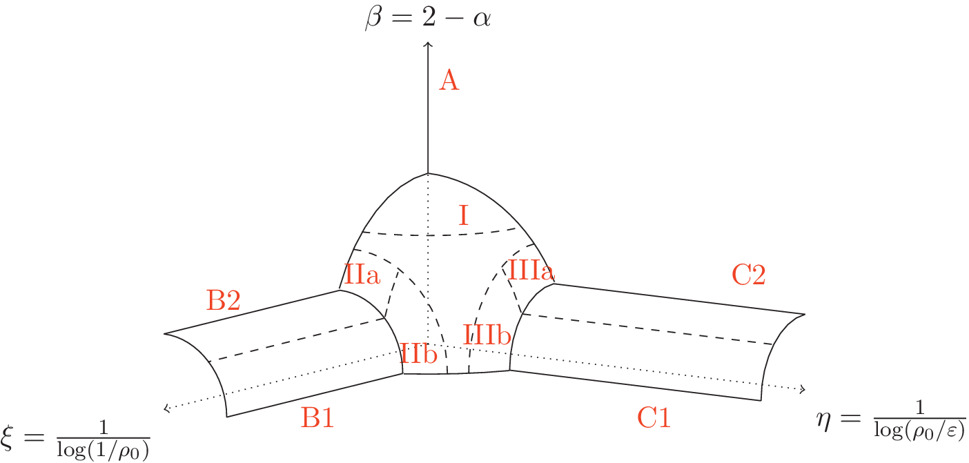

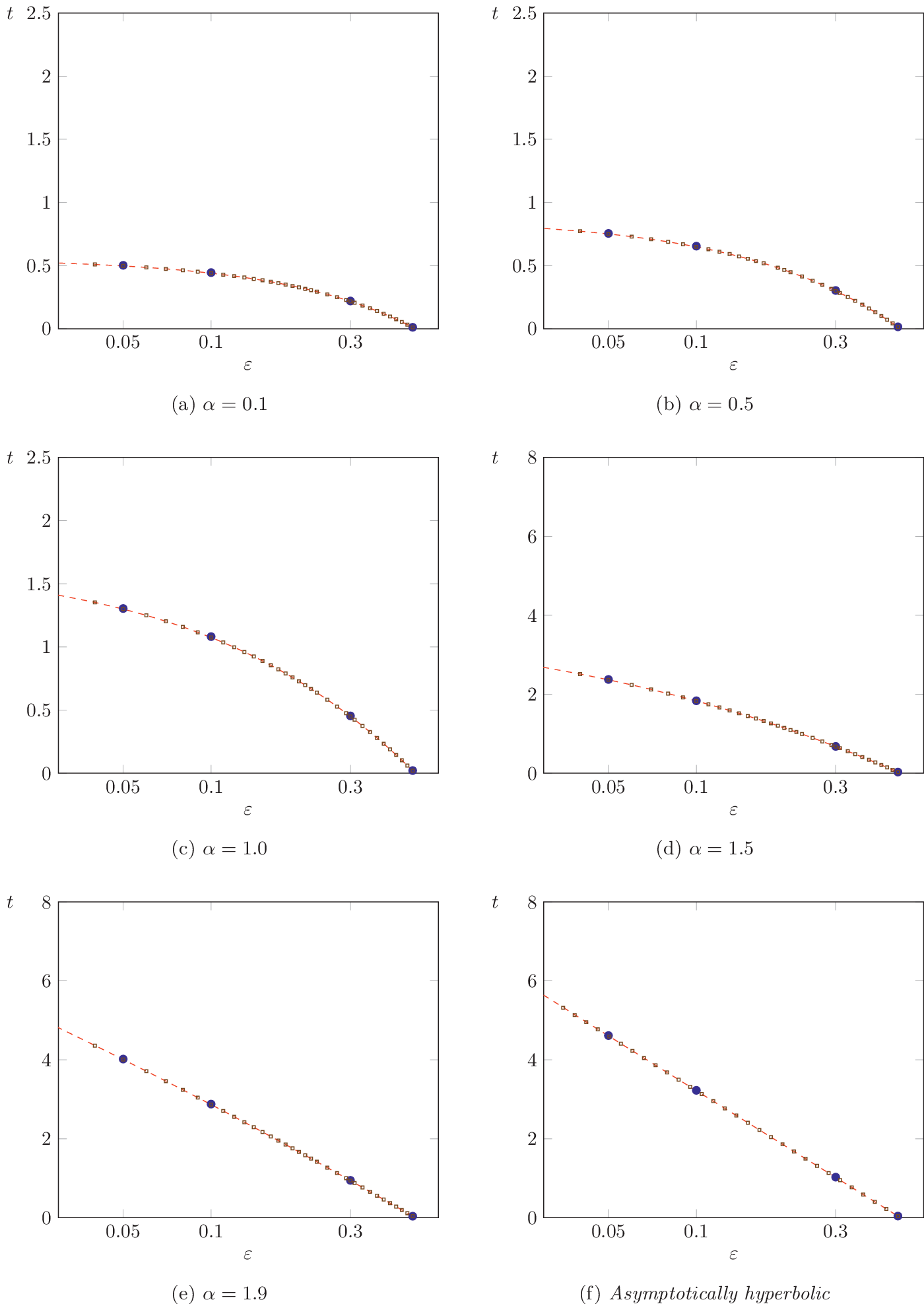


 Open access

