1. Introduction
Tearing modes (TMs) in tokamak plasmas (Wesson Reference Wesson2011) are notoriously difficult to characterize in terms of experimentally resolved features of tokamak equilibria (Bishop et al. Reference Bishop, Connor, Hastie and Cowley1991). This is unfortunate since TMs either initiate, or are a symptom of, chains of events leading to plasma disruptions, which need to be avoided in future reactor grade devices (de Vries et al. Reference de Vries, Johnson, Alper, Buratti, Hender, Koslowski and Riccardo2011). There is a vast literature on TM stability physics. Practical stability calculations with quantitative predictive capacity have not yet been demonstrated for arbitrary tokamak plasmas. Part of the reason for this is the assortment of TM onset mechanisms involved. The most fundamental ones are classical instabilities which may come in current-driven or pressure-driven varieties. The other main type is considered classically stable but which can be triggered by other nonlinearly evolving magnetohydrodynamic modes, perturbing sensitive aspects of the equilibrium configuration, leading to TM onset. Triggering mechanisms include edge localized modes and sawtooth oscillations (Wesson Reference Wesson2011). A third type of TM onset is radiation imbalances due to impurity accumulations (Gates & Delgado-Aparicio Reference Gates and Delgado-Aparicio2012). Even though the basic physics of these paths leading to TM onsets are established, the observed behaviour of a given real experimental plasma is likely to have an irreducible stochastic component. One reason for this is insufficient internal diagnostic resolution and measurement noise. Another reason is that near marginal stability, unpredictable plasma turbulence and thermal-fluctuation may effectively randomize the outcome. This suggests that there is value in approaching the TM onset problem using probabilistic modelling and machine learning to estimate the statistical regularities (Lawless Reference Lawless2002). Precise characterization of the rate of TM onset at given parts of physical feature space can provide useful information which otherwise would be difficult to obtain. Machine learning TM onset models can also be used as interpolation vehicles across the available database allowing completely new ways of searching and sorting plasma discharges. The topic of this paper is the initial development of capable database-wide association toolsets and techniques that are focused on quantifying and extracting information about the conditions for TM onset in the DIII-D tokamak.
The specific contributions of this work are: (i) automation of the labelling of TM onset events across a large subset of the DIII-D tokamak (Luxon Reference Luxon2002) database; (ii) principal component analysis of physics-motivated high-dimensional axisymmetric equilibrium features; (iii) the extension of TM onset hazard modelling to include both rotating mode onsets and locked mode onsets; and (iv) the first example demonstration of time-series TM hazard monitoring. All database-wide computations in this study use special fast-disk DIII-D database clone and parallel programming techniques (Moritz et al. Reference Moritz, Nishihara, Wang, Tumanov, Liaw, Liang, Elibol, Yang, Paul and Jordan2017; Sammuli et al. Reference Sammuli, Barr, Eidietis, Olofsson, Flanagan, Kostuk and Humphreys2018). The onset hazard modelling approach to TMs in tokamaks was introduced by Olofsson, Humphreys & La Haye (Reference Olofsson, Humphreys and La Haye2018). Prior work to extend the scale of the hazard modelling (Olofsson, Sammuli & Humphreys Reference Olofsson, Sammuli and Humphreys2019) was limited in that the labelling only included rotating TM onsets. The hazard modelling approach differs significantly from what is typically done for disruption prediction, which is a machine learning augmented research topic with a large body of literature (Pau et al. Reference Pau, Fanni, Carcangju, Cannas, Sias, Murari and Rimini2019; Rea et al. Reference Rea, Montes, Pau, Granetz and Sauter2020; Bandyopadhyay et al. Reference Bandyopadhyay, Barbarino, Bhattacharjee, Eidietis, Huber, Isayama, Kim, Konovalov, Lehnen and Nardon2021). Instead of attempting to model the probability of some future event, the hazard modelling attempts to produce a function that gives the instantaneous event onset intensity. In principle, such a function is a fundamental generator of the future event probabilities. Some of these ideas have been applied in disruption prediction research (Tinguely et al. Reference Tinguely, Montes, Rea, Sweeney and Granetz2019). The DIII-D tokamak has a strong track-record of research on TM stability (La Haye et al. Reference La Haye, Buttery, Guenter, Huysmans, Maraschek and Wilson2000; Buttery et al. Reference Buttery, La Haye, Gohil, Jackson, Reimerdes and Strait2008; Turco & Luce Reference Turco and Luce2010; Turco et al. Reference Turco, Luce, Solomon, Jackson, Navratil and Hanson2018; La Haye et al. Reference La Haye, Chrystal, Strait, Callen, Hegna, Howell, Okabayashi and Wilcox2022) and its database has unusually many examples from which to learn statistically. An important caveat with the underlying database is that magnetics-only equilibrium reconstructions need to be used to get excellent database coverage. This limits the resolution of internal details of the axisymmetric equilibrium features.
This report is organized as follows. Section 2 describes the non-axisymmetric magnetics diagnostics analysis schemes that are required to define a statistical learning problem. The output from these analysis tools is arguably the central deliverable in this work, as the information in the target variables and the implied analysis time windows drives the rest of the computation. Section 3 describes database-wide efficient single-pass principal component analysis and the pair of physics-motivated axisymmetric field features used for the statistical learning to follow is presented in § 4. Section 5 demonstrates two example applications of the fitted hazard function. The report is concluded with a discussion in § 6, which lists limitations and future improvements.
2. Magnetics analysis and labelling
This section provides an overview of the two types of magnetics analyses that are used to detect the onset of either rotating $n=1$ modes (RM) or locked $n=1$
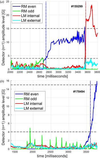
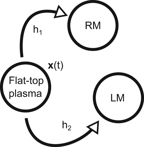
 modes (LM). The magnetics diagnostic instrumentation for the DIII-D tokamak is outlined in Strait (Reference Strait2006). The RM detector is based on coherent fluctuation analysis with windowed fast Fourier transforms (FFTs). The fundamentals of the RM detector method is summarized in Strait (Reference Strait2006) and references therein. The LM detector is based on a novel two-axis internal-external decomposition (Sweeney & Strait Reference Sweeney and Strait2019). Figure 1 shows examples of both RM and LM onset detection (in the same shot). Figure 3 shows a Markov chain illustrating how the onset detectors should be combined to model a total hazard function. This is described in more detail in § 2.4.
Example application of the RM (even/odd refers to poloidal mode number $m$ ) and LM event detector codes to magnetic signals. (a) DIII-D shot which exhibits an $n=1$
 mode that grows while rotating, then eventually locks. The RM detector catches the mode around $t=2.73\,\mathrm {s}$
 , and the LM detector catches it around $t=3.55\,\mathrm {s}$
 . The LM amplitude signal shoots up just as the RM amplitude signal disappears (mode locking). The respective detection levels are shown as dotted horizontal lines. The event detections are shown as dashed vertical lines. The RM odd trace and the LM external trace are intentionally ignored by the detectors. In a shot, the RM odd trace (green) presumably shows a sawtooth crash just before the growth of the RM even signature (blue). (b) More sustained ‘odd’ trace sawtooth activity and a rapidly growing mode emerging on the ‘even’ trace (later LM signal not shown). The same reference levels as in panel (a) are shown by the horizontal dashed lines.

2.1. Rotating mode (RM) detection
The RM onset detector uses fast-sampled (mostly $200.0\,\mathrm {kHz}$ ) non-integrated (measuring band-limited $\mathrm {d}B/\mathrm {d}t$
 ) magnetic probe array data. Rotating $n=1$
 mode signatures in DIII-D are typically at ${\sim }10\,\mathrm {kHz}$
 and below. In the analysis used in this work, ten midplane magnetic probes are employed, of which nine are located on the outboard side, and one is located on the inboard side. The inboard probe is important in that it allows distinguishing between sawtooth oscillations, which are also $n=1$
 , and TMs. The outboard probes are approximately distributed evenly along the outboard perimeter.
The signal processing algorithm is based on finding coherent fluctuation frequencies associated with a specified spatial wavelength, matching that of a $n=1$ mode. The analysis is implemented as a filter that maintains a running estimate of the short-time power spectrum of each probe signal and the cross-spectra of pairs of probe signals. The FFTs are fed data pre-processed with mean removal and Hamming windowing. The algorithm uses cross-spectra between a probe and its neighbour (the next toroidal coordinate). An additional cross-spectrum is needed for the inboard probe and its nearest outboard neighbour (at approximately the same toroidal coordinate). The resulting information is used to compute array-averaged coherences (robustified by removing smallest amplitude and highest amplitude probes). The magnitude and phase of the coherence is used to extract information about the rotating modes. Specifically, the phase of the coherence spectra can be divided by the real-space toroidal angle separation to estimate the RM $n$
 -number, which must be sufficiently close to $1$
 (assuming that the magnitude of the coherence is sufficiently high). In the case where coherent fluctuations are isolated, the amplitude of the corresponding RM can be estimated by a weighted sum across the power spectrum bins (only counting the isolated frequency assumed to be due to $n=1$
 ). The coherent fluctuation amplitude is apportioned to either the odd or even trace (‘odd’ and ‘even’ refer to the spatial $m$
 number) based on the complex phase of the cross-spectrum for the special inboard–outboard probe pair.
An example application of the RM code is displayed in figure 1(a) (blue and green traces). It is seen that the estimated amplitude level for the RM (due to the above algorithm, which only sees non-integrated $\mathrm {d}B/\mathrm {d}t$ ) is consistent with the initial locked mode amplitude level (which is inferred using a very different algorithm, using integrated magnetic field measurements ${\sim }B$
 , at a much lower sample rate). Generally, as the RM speed of rotation decreases, this method works less well. Sub-$\mathrm {kHz}$
 signals are difficult to analyse with this technique. In figure 1(a), it is seen that the volatility of the amplitude estimate appears to increase shortly before the RM signal dies off completely (just before locking). Figure 1(b) shows a different case that exemplifies how the ‘odd’ trace consistently captures the sawtooth oscillations, while the ‘even’ trace captures a rotating mode that grows rapidly. Eventually, this RM signal dies off and the TM locks also in this discharge around $t=3.91\,\mathrm {s}$
 (not shown).
2.2. Locked-mode (LM) detection
The LM onset detector is using two types of magnetic diagnostics: (i) saddle loops measuring radial magnetic field averages; and (ii) probes measuring tangential magnetic fields. Both (i) and (ii) are integrated by analogue electronics before digitization. A total of eight radial measurement signals and ten tangential measurement signals are used. Each signal originates from a pair-difference of two actual physical probes (Strait Reference Strait2006). Optionally, a set of $18$ active coil current measurements (associated with driven saddle coils) can be used to ‘compensate’ the $18$
 distinct measured signals. Typical sample frequencies for the $18$
 LM detection signals are 20.0 and $50.0\,\mathrm {kHz}$
 . In contrast to the RM analysis, the LM analysis is sensitive to drifts and offsets in the signals. A practical method to handle these slowly changing offsets is to use a ‘dynamic rebaselining’ scheme (Strait, Munaretto & Sweeney Reference Strait, Munaretto and Sweeney2019). In this analysis, a one-pole filter with time constant $\tau _b$
 is used to maintain a running average level for each magnetic measurement included. The dynamic baseline level is defined as the running average, delayed by a time $\tau _d$
 . The rebaselined signal is then defined by subtracting the dynamic baseline (filtered, delayed) from the original magnetic measurement. The effect of this scheme is that abrupt transients are preserved, while slowly drifting offsets (of any kind) are suppressed. Here, the values $\tau _b=100\,\mathrm {ms}$
 and $\tau _d=100\,\mathrm {ms}$
 were employed. If ‘compensated’ signals are used, then the original measurement is redefined by subtracting the known instantaneous coupling from active coils to each sensor. If the active coils carry DC-only currents, this may improve the analysis.
The rebaselined signals are then interpreted using an ordinary least-squares estimation procedure. Based on the known geometry of the sensor array, a matrix $K$ can be defined that links a set of sine, cosine modes to the measurements. The estimation matrix $M$
 is defined by the standard normal equations $M=(K^{\rm T} K)^{-1}K^{\rm T}$
 . In this work, only the rows of $M$
 that are associated with the $n=1$
 internal and external sine and cosine components are used (the matrix also contains $n=2$
 , $n=3$
 ). In case some measurements are missing from a shot, the estimation matrix is regenerated by deleting the corresponding rows of $K$
 (the full $K$
 has $18$
 rows and $12=3\times 4$
 columns). Cosine $c_{n=1}$
 and sine $s_{n=1}$
 coefficients for the estimated $n=1$
 fields (internal and external, respectively) are combined with mode amplitude estimates in the usual sense $\hat {A}_{n=1}=\sqrt {c_{n=1}^2 + s_{n=1}^2}$
 .
An example application of the LM code is displayed in figure 1(a) (red and cyan traces). The abrupt LM event for the internal amplitude signal (red) is clear and follows just after the RM trace (blue) vanishes. Notice that after a time $\tau _d$ has passed since the LM event, the event itself starts to creep into the rebaselining scheme. So the drop in amplitude of the red trace from its peak is likely an artefact of the dynamic rebaselining, and this scheme should not be used for detailed analysis of the mode post-locking (which does not apply to the present analysis). This scheme is only used to detect the LM event transient itself (but the rebaselining could be freezed when an event is detected) in the presence of various drifts and offset levels (and it can be incorporated in real-time in plasma control systems for mode-locking detection). Notice how the noise-levels for the LM traces are approximately the same in amplitude as the typical ‘odd’ trace signals from the RM code in figure 1(a,b), but well below its threshold value, here set to $15.0\,\mathrm {G}$
 .
2.3. Threshold-count curves for RM and LM detectors
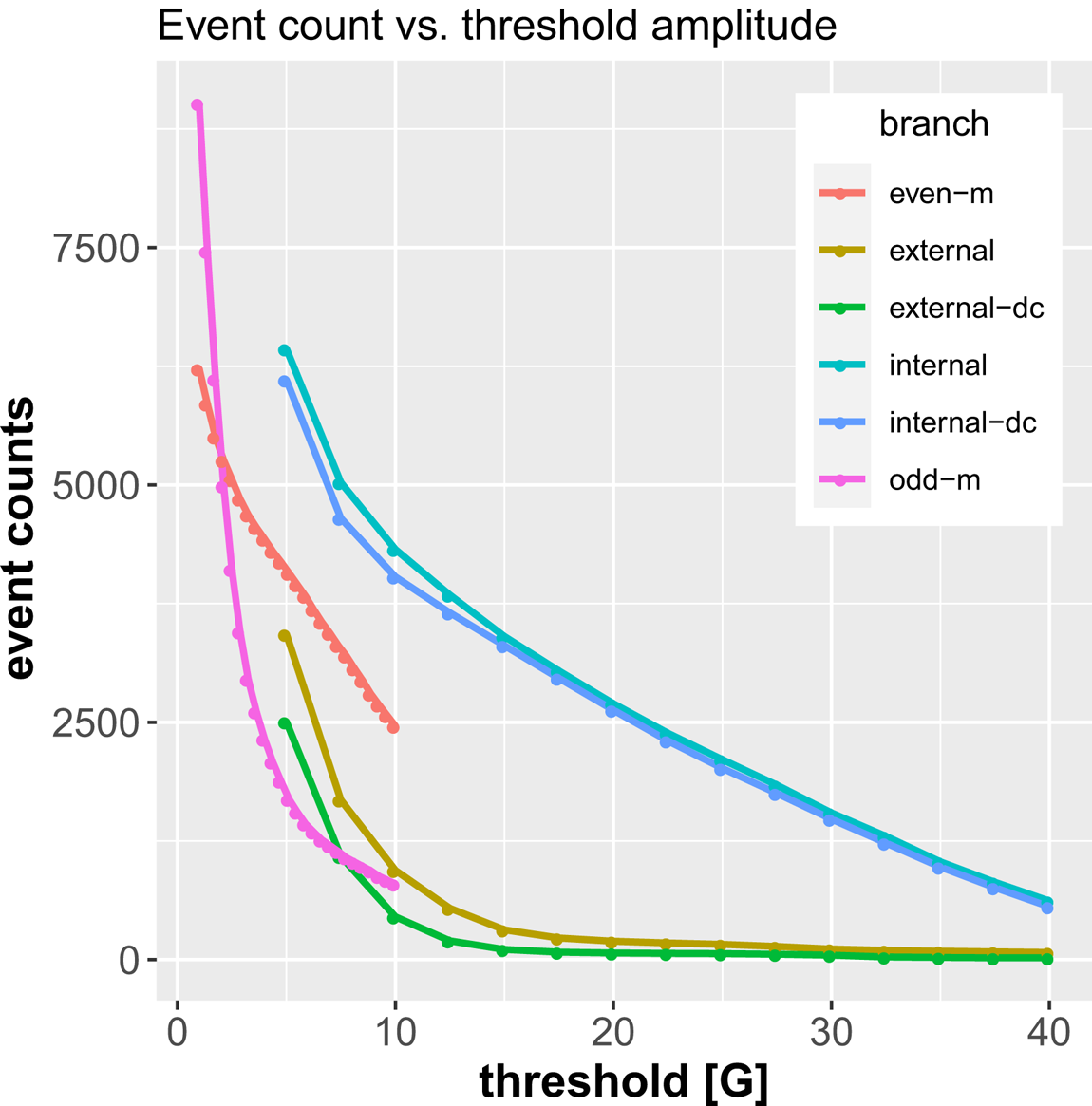
Figure 2 shows the number of detected events as a function of the event threshold amplitude level. There are a total number of six different amplitude traces generated by the RM and LM codes. The RM code produces $n=1$ ‘even’ and ‘odd’ traces. The LM code produces the $n=1$
 ‘internal’ and ‘external’ traces. The LM code can be run either with or without DC compensation. The RM ‘odd’ trace gets tripped on small amplitude activity mostly associated with sawtooth fluctuations. These typically are found at or close to the rotational frequency of the $n=1$
 TMs, and separating these from the RM even trace significantly improves the RM detector specificity.
Number of events caught across the database for the four different branches of $n=1$ amplitude traces. The RM analysis code provides ‘even’ and ‘odd’ traces, of which the odd trace mainly captures sawtooth activity at low amplitude, which is ignored. The LM code produces ‘internal’ and ‘external’ amplitude traces. Both these traces are computed in two different ways: uncompensated and DC compensated (meaning that active coil currents were explicitly fetched and known couplings were subtracted).

In this work, the RM detector threshold is at $4.0\,\mathrm {G}$ (even trace only, odd trace ignored) and the LM detector threshold is set at $15.0\,\mathrm {G}$
 . These values are selected based on both (i) examples such as figure 1 and (ii) the global statistics shown in figure 2. The RM detector level appears to be mostly free of sawtooth influence but still not so high as to ignore many potentially low-amplitude RMs. If the RM threshold is too high, the event time can also move far away from the actual onset time. The LM detector level chosen appears to be high enough to avoid potential influence from transients that show up on both the internal and external traces. Such transients are likely not due to an actual LM of interest, which should be found only on the internal trace. Additionally, the difference between the DC-compensated and uncompensated event detection statistics start to become very small at the selected threshold and above, suggesting that the effect of active coil transients is not a concern at that level.
At the selected thresholds, the RM and LM detections are compared in detail by checking the joint results for the same plasma discharges. The number of shots where both detectors ran, in this study, is 18 026 (subset of shots in the DIII-D database range #155 001–#187 977). In 12 226 of these doubly analysed shots, there was no event found by any of the detectors. In $2506$ of the shots, only the RM event was detected. In $1389$
 of the shots, only the LM event was detected. In $1905$
 of the shots, both the RM and the LM detectors triggered, but in $1707$
 (of the $1905$
 ), the RM event preceded the LM event in the same shot. These results are consistent with the expectation in that (i) many times RMs never lock (lots of torque injected into the plasma, or RM too small), (ii) LMs can develop with no prior RM (born locked), or its RM is very short-lived, rotates slowly or both, and therefore is not detected, and (iii) the common sequence of events is otherwise that an RM appears, grows, locks, then its LM signature is detected (Fitzpatrick Reference Fitzpatrick1993). Both example events in figure 1 are of this common type. In some cases, a mode could be born locked and then spun up and subsequently be detected as an RM (i.e. LM preceeding RM). Alternatively, there could be detection errors. Whatever the reason, the event that comes first will be used to define the TM onset, as explained in § 2.4. Notice that the total number of shots with both RM/LM detector data runs and the availability of suitable equilibrium reconstructions (next section) is somewhat smaller (17 178 in this study).
2.4. Preparing a jointly labelled dataset (RM and LM)
Figure 3 shows a representation of the probabilistic model relevant for the present work. The dataset to be prepared should reside in the pre-event flat-top state. Any RM or LM event, whichever comes first, terminates this pre-event flat-top state. The respective probabilities of events of type RM, LM are $h_1/(h_1+h_2)$ , and $h_2/(h_1+h_2)$
 (assuming these values were known). The hazard modelling in this work attempts to estimate a function for the total hazard $h=h_1+h_2$
 , which defines the jump-intensity out of the pre-event flat-top plasma state. For the plasma example shown in figure 1(a), the relevant data preparation then becomes that of cutting away all data after the RM onset is detected (and not using the LM detection result). The data from this shot will be included up to time $t=2.73\,\mathrm {s}$
 , and only its final time slice will be marked as being an ‘onset event’. For any shot where neither an RM nor LM onset is detected, its data will be included for the full flat-top, and all time-slices are non-events/normal. Although RM and LM events are distinct from the perspective of the detector, this construction of the total hazard combines both types of detections into a single event rate. This is done purposefully as the RM and LM are seen as manifestations of a single underlying TM event.
Continuous-time Markov model with two absorbing states: RM and LM. The respective jump rates from the pre-event flat-top state are $h_1$ and $h_2$
 . The hazard function in this work directly models the sum of these jump rates: $h = h_1 + h_2$
 . With the sum-total $h$
 as the learning objective, the data from each shot should be prepared up to the occurrence of either the RM or LM event, whichever comes first, or in the case of no event, cut off at the end of the discharge flat-top.

After the data have been prepared as outlined above, each pre-event flat-top time-slice will have a feature vector (covariate vector) $\boldsymbol {x}(t)$ associated with it. The data are now used to define a specific statistical estimation problem (or machine learning problem): approximate a function $h(\boldsymbol {x})$
 that maps the covariate $\boldsymbol {x}(t)$
 to the most probable instantaneous hazard rate. The function is not given access to the value of the time $t$
 , only the present value $\boldsymbol {x}$
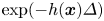
 of the covariate vector, which is supposed to contain information about the relevant physical state. The feature generation is detailed in § 3, whereas the statistical modelling is detailed in § 4. The learning problem is mapped to the standard binomial likelihood by noting that the survival probability across a small time-step $\varDelta > 0$
 can be defined as $\exp (-h(\boldsymbol {x})\varDelta )$
 (Olofsson et al. Reference Olofsson, Humphreys and La Haye2018). Consequences of this small-step property are further explored in Appendix B.
3. Feature processing and dimensionality reduction
This section details a practical principal component analysis (PCA) of a pair of field features related to the distribution of magnetostatic self-energy associated with the axisymmetric equilibrium. The underlying data are derived from the standard magnetics-only equilibrium reconstruction for the DIII-D database (Lao et al. Reference Lao, John, Stambaugh, Kellman and Pfeiffer1985). It is generally accepted that this does not meaningfully resolve the internal current density distribution. However, the general plasma shape is well characterized, as are basic descriptors, such as the normalized pressure and global inductances. Further comments about this are found in § 6.
Notice that the PCA dimensionality reduction algorithm is used in a standard unsupervised way, i.e. there is no reference to the onset event information in this feature processing step. The PCA achieves a sorting of the feature data according to variance along principal vectors (this sorting may or may not be associated with signal versus noise). The combination of the unsupervised PCA with model fitting and selection is the topic of § 4.
3.1. Scaleable computation of feature basis vectors
The calculation of the database-wide PCA basis for a feature is arranged as follows. Let $\boldsymbol {x}$ be a vectorized instance of the feature of interest (the values on the grid of some EFIT-derived quantity taken as a column vector). All available worker processes are given a batch of shots. The batches are created by shuffling the available shots randomly and partitioning the shuffled list into disjoint sets of approximately equal size. The shuffling makes the time required to process each batch the same on average (each shot has a variable number of time slices associated with it). As each worker finishes a batch, it receives a yet unprocessed batch, until all batches have been processed. For each finished batch $b$
 , the worker returns three objects back to the calling process: (i) the number of time slices $n_b$
 that was used for all shots in the batch; (ii) the mean feature $\langle \boldsymbol {x} \rangle _b$
 ; and (iii) the mean outer product $\langle \boldsymbol {x} \boldsymbol {x}^{\rm T} \rangle _b$
 . The calling process maintains the total statistical information $(n, \langle \boldsymbol {x} \rangle, \langle \boldsymbol {x}\boldsymbol {x}^{\rm T} \rangle )$
 by assimilating the incoming results (in any random order) using the update program

where $\alpha = n / (n + n_b)$ and $\beta = n_b / (n + n_b)$
 , and $\leftarrow$
 denoting assignment. Notice that the individual features $\boldsymbol {x}$
 are calculated by the workers on-the-fly and not returned or stored (due to memory constraints).
When the parallel aggregation is done, a symmetric eigenvalue decomposition (EVD) is computed for the (centred) matrix

and the first few columns of the orthonormal $V$ are used as the basis set for the feature of interest, assuming the EVD has been sorted so that $\varLambda$
 has decreasing diagonal elements $\lambda _{i+1} < \lambda _i$
 . This PCA basis calculation only requires one single pass over the database.
Denote the first $k$ columns of $V$
 by $V_k$
 . The reduced representation of a feature $\boldsymbol {x}$
 is then computed as

where $\boldsymbol {z}$ is a $k$
 -dimensional vector of coefficients that specify the offset from the mean feature, along the dominant principal axes of the covariance matrix. Computation of (3.3) requires a second pass over the database, since each specific feature $\boldsymbol {x}$
 need to be recalculated and $V_k$
 is unknown in the first pass. The reduced vector can be used to approximate the full feature again as

where the reconstruction error $\|\boldsymbol {x}_{\mathrm {rec}} - \boldsymbol {x}\|_2^2$ is bounded by the sum of the trailing eigenvalues $\sum _{i=k+1}\lambda _i$
 (in a statistical sense). Denote the full sum $\varGamma \equiv \sum _j\lambda _j$
 . The dimension cutoff $k$
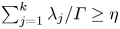
 is usually determined as the smallest integer satisfying a condition $\sum _{j=1}^k \lambda _j / \varGamma \geq \eta$
 , where $\eta = 0.995$
 or similar. The computational modelling that follows works with the adimensional feature vectors

so that the joint treatment of different features has a standard numerical scale. In what follows, this is important for the logistic linear regression modelling, but does not matter for the particular type of nonlinear learning machine applied.
The EVD (3.2) can be related to an equivalent singular value decomposition (SVD) as follows. Let all the samples be collected in a matrix $X$ , each row being a sample. Here, $X$
 has $N \sim 2.5\,\mathrm {M}$
 rows and $4225$
 columns. Let $\boldsymbol {1}$
 be a length-$N$
 column of ones. Disassemble $X$
 into two terms $X = \boldsymbol {1}\langle \boldsymbol {x}\rangle ^{\rm T} + \tilde {X}$
 , so that $\tilde {X}$
 has zero-sum (zero-mean) columns $\boldsymbol {1}^{\rm T}\tilde {X}=\boldsymbol {0}^{\rm T}$
 . It follows that $(1/N)X^{\rm T} X=\langle \boldsymbol {x}\rangle \langle \boldsymbol {x}\rangle ^{\rm T} + (1/N)\tilde {X}^{\rm T} \tilde {X}$
 . So the right-hand side of (3.2) is equal to $(1/N)\tilde {X}^{\rm T} \tilde {X}$
 (sample covariance matrix). Given the SVD of the centred data matrix $\tilde {X}=U S V^{\rm T}$
 , it follows that $(1/N)\tilde {X}^{\rm T} \tilde {X} = V (S^2/N) V^{\rm T}$
 , so the singular values $\sigma _i$
 (diagonal of $S$
 ) are related to the eigenvalues as $\lambda _i = \sigma _i^2 / N$
 .
3.2. Calculation and properties of ${J}\,{\cdot }\,{A}$

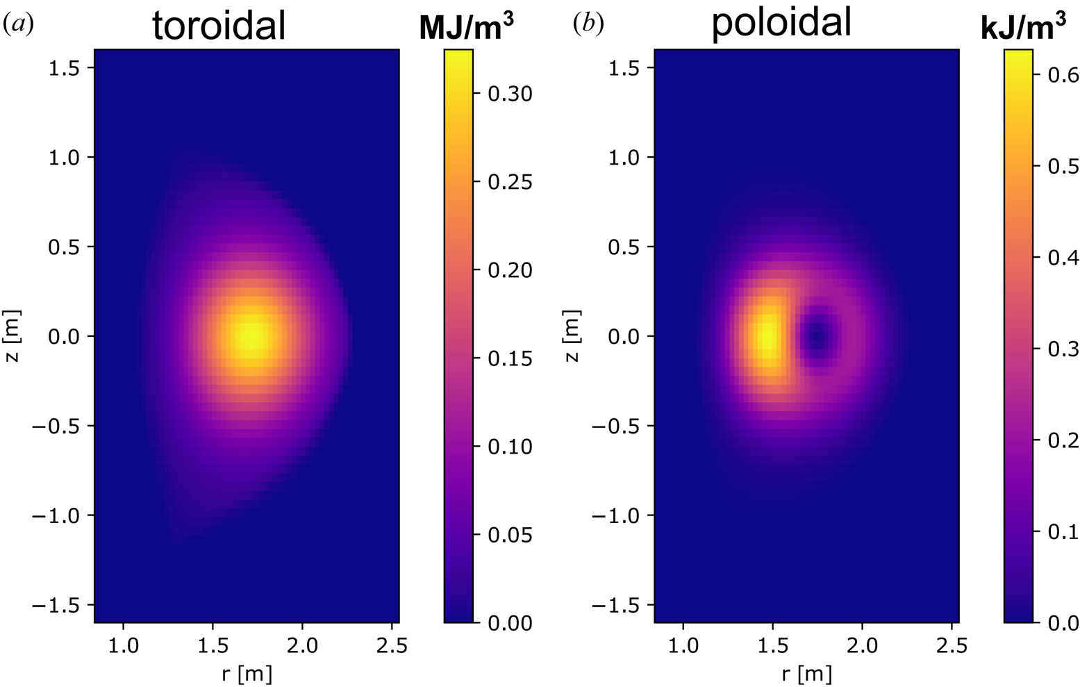
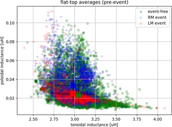
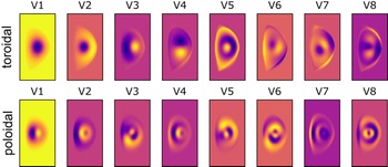
The field feature being explored in this work, and described in this subsection, has several justifications. The feature carries information about plasma shape and distributions in both toroidal and poloidal directions. The feature visually look like the current density which is favourable for interpretation. Its integral represent magnetostatic energy, and it is part of the Lagrangian for magneto-mechanical systems, such as the macroscopic stability of tokamak plasmas. Gradients of the Lagrangian in principle decide the stability (although it is unclear whether that theoretical property can be meaningfully exploited in this context). The form used here generates positive-valued features regardless of the sign of the plasma current or the toroidal magnetic field. This makes the PCA mean feature $\langle \boldsymbol {x} \rangle$ more meaningful. This feature has compact support (the distribution of plasma-associated current density) and the circuit self-inductances derived from it are correlated with standard quantities such as the internal inductance $\ell _i$
 and the poloidal beta $\beta _p$
 . The database-wide mean feature pair (defined below) is depicted in figure 4. The flat-top averaged operating space in terms of the associated scalar summary pair $(L_{\mathrm {tor}}, L_{\mathrm {pol}})$
 (also defined below) is shown in figure 5. The first few orthogonal PCA basis vectors for the feature pair, calculated as detailed in § 3.1, is shown in figure 6. In what follows, $r$
 , $z$
 and $\phi$
 denote the coordinates in the usual cylindrical system, where $\phi$
 is the toroidal symmetry angle. The axis of rotation is at $r=0$
 , $z$
 is the axis-parallel coordinate and $z=0$
 has no special meaning except it is usually defined to be at the nominal midplane of the tokamak chamber. The axisymmetric fields are distributions in $(r,z)$
 space which hold their value for all $\phi$
 .
Database-wide pair of mean energy-based features. (a) Toroidal mean feature $\langle \boldsymbol {x} \rangle$ , where $\boldsymbol {x}$
 is the toroidal term $f_{\mathrm {tor}}$
 of $(1/2)\boldsymbol {J}\boldsymbol {\cdot }\boldsymbol {A}$
 . (b) Mean feature when instead, $\boldsymbol {x}$
 is the poloidal term $f_{\mathrm {pol}}$
 of $(1/2)\boldsymbol {J}\boldsymbol {\cdot }\boldsymbol {A}$
 . Approximately $2.5$
 million equilibrium reconstructions were used in the analysis, accrued from $17\,000$
 different DIII-D plasma discharges.

Scatter plot of the pre-event flat-top averages of the circuit self-inductances defined by (3.10) and (3.11). The set of discharges is partitioned into three sets: those where there was no onset event anywhere (green), those that have an RM onset (blue) and those that have an LM onset (red). The correlation coefficient between $L_{\mathrm {tor}}$ ($L_{\mathrm {pol}}$
 ) and $\ell _i$
 ($\beta _p$
 ) is $0.76$
 ($0.65$
 ) for this dataset. The TM onset events are distributed across this average operating space, with only small differences. The mean for each set is marked by a coloured square. The cross-hairs through each mean marker shows the quantile range $(0.10, 0.90)$
 for the marginal distributions associated with each set.

Database-wide PCA basis vectors. The top row shows the first eight orthonormal vectors for the toroidal feature. The bottom row shows the first eight orthonormal vectors for the poloidal feature. The first vector in both rows is largely (anti-)parallel to the respective mean feature (cosine similarities $-0.99$ and $-0.98$
 ). The colour-scale is adapted to each thumbnail independently. The basis vectors are the columns of the matrix (3.2) for the respective feature (toroidal and poloidal).

The field $(1/2)\boldsymbol {J}\boldsymbol {\cdot }\boldsymbol {A}$ represents magnetostatic configuration energy density, as long as the Coulomb gauge is used, which can be enforced by requiring $\boldsymbol {\nabla }\boldsymbol {\cdot }\boldsymbol {A} = 0$
 . This magnetic vector potential $\boldsymbol {A}$
 is not typically computed or stored in standard databases of equilibrium reconstructions. Instead, it is here computed as-needed, as the features are required in the passes across the database. It is done as follows. The plasma current density $\boldsymbol {J}$
 triad ($J_{\phi }$
 , $J_{r}$
 , $J_{z}$
 ) is produced from the stored equilibrium reconstruction ($J_{\phi }(r,z)$
 is a field of scalar values on the same grid in $(r,z)$
 as the underlying equilibrium reconstruction, and so on). Specifically, representations for $J_{\phi }(r,z)$
 and $B_{\phi }(r,z)$
 can be generated directly by mapping stored information, and $J_{r}$
 , $J_{z}$
 can be defined through $\mu _0 J_r = -(1/r)\partial _z (r B_{\phi })$
 and $\mu _0 J_z = (1/r)\partial _r (r B_{\phi })$
 using finite differencing. For numerical consistency, this specific $\boldsymbol {J}(r,z)$
 is used as the input to (source term for) the remainder of the calculation, in the end, allowing the calculation of $\boldsymbol {J}\boldsymbol {\cdot }\boldsymbol {A}$
 , where $\boldsymbol {A}=\boldsymbol {A}(\boldsymbol {J})$
 . The toroidal component of the vector potential ($A_{\phi }$
 , $A_{r}$
 , $A_{z}$
 ) is obtained by solving

on the same grid, with $\varDelta ^{*}a=r\partial _r((\partial _r a)/r) + \partial ^2_{zz}a$ , where the boundary condition is defined using the right-hand side source and the known Green's function for this elliptic operator. Multiplying (3.6) by $2{\rm \pi}$
 yields the familiar equation for the poloidal flux function $\psi = 2{\rm \pi} r A_{\phi }$
 . The poloidal vector potential components can be solved by mapping to the very same (3.6) with a different source term and some post-processing. This mapping is further detailed in Appendix A. Specifically, solve

where $I_z(r,z)$ is an integral current function defined from $J_z(r,z)$
 as $I_{z}(r,z) = \int _0^r {\rm d} r^{\prime } 2{\rm \pi} r^{\prime } J_z$
 . The right-hand side in (3.7) is equal to $-rB_{\phi }$
 , with $B_{\phi }$
 being the poloidal plasma current generated toroidal field. The poloidal part of the vector self-potential can be computed as streamlines of the solution to (3.7)

and based on (3.6), (3.7), the features used in this work are the two terms $f_{\mathrm {tor}}$ , $f_{\mathrm {pol}}$
 in the decomposition

which are further dimensionality reduced as detailed in § 3.1. The integral $U = (1/2)\int \mathrm {d}V\boldsymbol {J}\boldsymbol {\cdot }\boldsymbol {A}$ is the all-space field energy associated with the source distribution $\boldsymbol {J}$
 . Two useful scalar reductions of these field features are plasma self-inductances $L$
 , defined by relationships $U=(1/2)LI^2$
 . The toroidal circuit self-inductance is

where $I_{\phi } = \int {\rm d} r\,{\rm d} z J_{\phi }$ and $\mathrm {d}V=2{\rm \pi} r \,{\rm d} r\,{\rm d} z$
 . Let $I_{\mathrm {pol}}=\max _{r,z}I_z$
 , then the poloidal circuit self-inductance is similarly defined by

and the space $(L_{\mathrm {tor}}, L_{\mathrm {pol}})$ is a two-dimensional reduction that depends only on the circuits traced out by $\boldsymbol {J}$
 . These self-inductances are used as axes in the scatter plot of the database shown in figure 5. Here, $L_{\mathrm {tor}}$
 carries information about poloidal magnetic fields (toroidal current loops), whereas $L_{\mathrm {pol}}$
 carries information about toroidal magnetic fields (poloidal current loops). Notice that the events and non-events are scattered in this space similar to each other, with no clear tendency of separation.
Numerically, discretized (3.6), (3.7) are solved as general Sylvester equations $EX+XF=G$ , where $X$
 is the unknown matrix of field values, shaped as the grid, and $E$
 , $F^{\rm T}$
 represent the elliptic operator separated in $r$
 , $z$
 , and $G$
 combines boundary and source data. A standard general-purpose Sylvester solver is used which does not assume any specific structure to $E$
 , $F$
 .
4. Linear and nonlinear hazard modelling
This section begins by developing a principal component linear logistic regression (PCLLR) model for the hazard rate. This basic modelling technique can be used to graphically indicate what aspects of the high-dimensional feature set tend to be associated with more or less tearing onset rates. The model can be fitted directly on the entire dataset if a rigorous model selection technique is used, which is imported from the literature on statistical estimation. In addition to being a vehicle for visual interpretation, the PCLLR model also serves as a benchmark against which more powerful nonlinear learning machines can be compared. The third subsection describes the usage of certain configurations of gradient boosting machines applied to the hazard onset estimation. Finally, the linear and nonlinear models are compared not only in terms of cross-entropy fitness to event data, but also by sampling their respective calibration curves across a fixed quantile range of their outputs.
4.1. Principal component linear logistic regression and model selection
A linear logistic regression model in the principal component feature space can be fitted on the full dataset using second-order optimization. It is beneficial to use the PCLLR model as a well-defined performance benchmark to compare against more complex and harder to interpret learning machines. The PCLLR model is specified by an intercept term $\beta _0$ and a coefficient vector $\boldsymbol {\beta }=(\beta _1,\ldots,\beta _m)$
 . The number of coefficients is equal to the sum of the truncated dimensions from the PCA basis sets: $m=n_1+n_2$
 . Specifically, $n_1$
 ($n_2$
 ) is equal to the truncation order $k$
 in (3.3) for the toroidal (poloidal) feature field. The PCLLR model evaluates a linear combination of the available features $\tilde {\boldsymbol {z}}$
 , and puts the resulting scalar (the log-odds value, $f(\tilde {\boldsymbol {z}})$
 )

through a sigmoid transformation

to get the probability $p(\tilde {\boldsymbol {z}})$ . The reverse operation is $f = \log [ p/(1-p) ]$
 , hence its name. The hazard is obtained through a different transformation of the log-odds value

that uses the average time range $\varDelta$ with which the examples are associated. Equation (4.3) follows from equating the small-time interval survival probability to the hazard $h$
 , $1-p = \exp (-\Delta h)$
 , handling $h$
 as the parameter of an exponential random variate. Only the first of these relations, (4.1), changes if another learning machine is used. Different PCLLR models can be compared using a specialization of the very general evidence procedure, based on a Laplace approximation of the mode of the likelihood function (MacKay Reference MacKay2003). The model fitting and selection procedure centres around three terms (in logarithmic scale). First, the (data) likelihood term

is larger the better the model fits the dataset. Second, the (regularizing) prior term

penalizes models which are too ‘extreme’. Specifically, the coefficient vector $\boldsymbol {\beta }$ is treated as if drawn from a prior normal distribution $\boldsymbol {\beta }\sim \mathrm {N}(\boldsymbol {0}, \varSigma )$
 , where the covariance matrix $\varSigma$
 is parametrized appropriately (see § 4.2) by some parameter $\boldsymbol {\theta }$
 . The quadratric form can be recast as $(-1/2)\sum _j r_j^2$
 , where $L\boldsymbol {r}=\boldsymbol {\beta }$
 , using the Cholesky factor $\varSigma = LL^{\rm T}$
 , and $l_{\varSigma, jj}$
 is the $j$
 th diagonal element of this $L$
 . Now $\boldsymbol {\beta }$
 is efficiently optimized for any fixed tuple of (hyper-)parameters $(\boldsymbol {\theta }, n_1, n_2)$
 by a Newton-like method (Murphy Reference Murphy2012), only considering the first terms $\mathcal {L}_1+\mathcal {L}_2$
 . The Hessian at the optimum gives the information required to evaluate the third term $\mathcal {L}_3$
 . The third term

where $l_{H,jj}$ is the $j$
 th diagonal entry of the Cholesky factor of the Hessian matrix evaluated at the minimizer of $-\mathcal {L}_1-\mathcal {L}_2$
 (the Newton-like solver), essentially penalizes the volume of available parameter space (MacKay Reference MacKay2003). This term limits the complexity of selected models and should, in principle, be used when comparing models with varying number of parameters (Murphy Reference Murphy2012). The Hessian information at the optimum can also be used to extract standard confidence intervals for the fitted PCLLR parameters (and, more generally, it can be used to generate approximate posterior samples).
The full model fitting and selection scheme can be summarized as

where the two truncation orders ($n_1$ , $n_2$
 ) respectively refer to the retained dimension of the toroidal and poloidal features, and $\boldsymbol {\theta }$
 is the parameter defining the prior covariance for $\boldsymbol {\beta }$
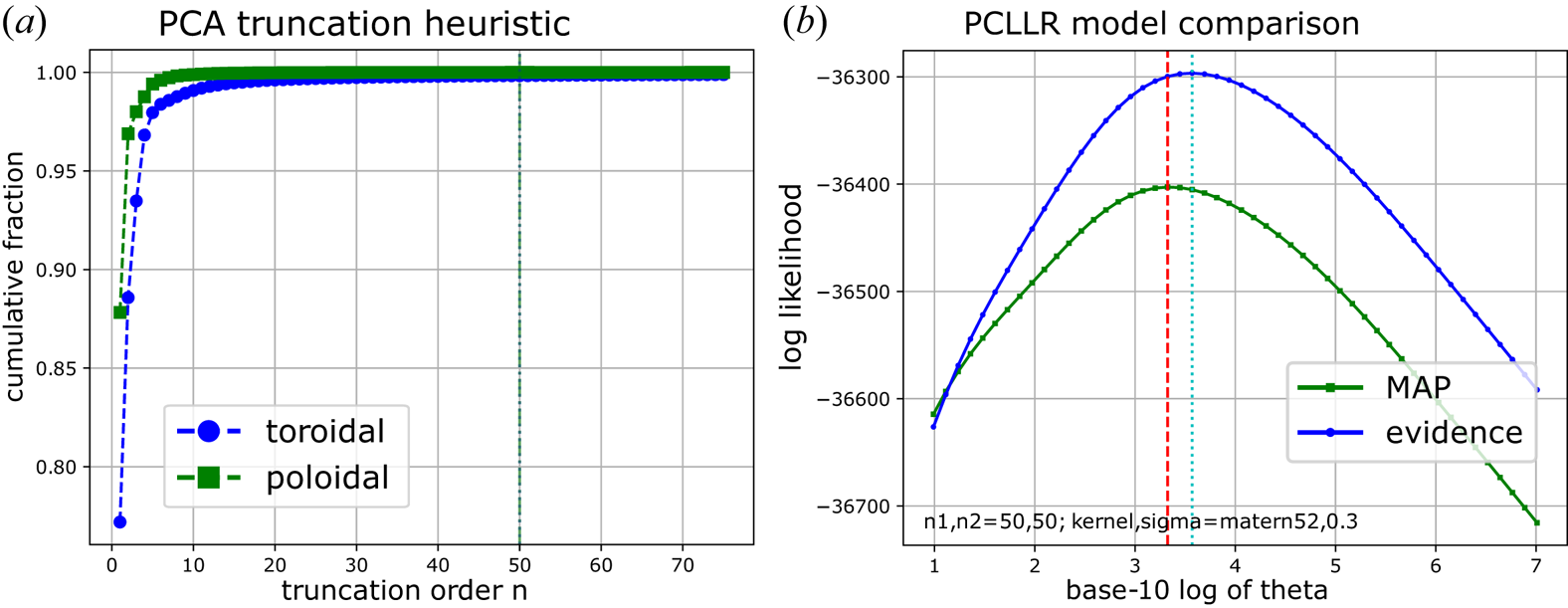
 (see next subsection). Model selection using heuristic PCA truncation combined with ‘evidence’ maximization (4.7) is illustrated for the PCLLR model in figure 7(a,b). The problem is simplified by first setting the PCA basis set ‘large-enough’ and then optimizing the most important hyper-parameter. It is possible to include all the parameters, including the truncation orders, in the selection programming (4.7) but it becomes computationally demanding and it is arguably not worth the effort since the results are similar and the PCLLR model is limited in capacity anyway (as will become clear by comparing its calibration curves below). In § 4.5, the model selection expressions are evaluated as a function of the PCA cutoff (to compare different features). Figure 11 generally suggests an effect of ‘diminishing returns’ for increasing cutoff at $n_1 = n_2 = n\sim 50$
 , information impossible to tell by figure 7(a) alone. Each trace in figure 11 corresponds to maximizations as illustrated in figure 7(b).
Model selection based on (a) heuristic PCA truncation and (b) optimization of either $\mathcal {L}_1 + \mathcal {L}_2$ (green trace) or $\mathcal {L}_1 + \mathcal {L}_2+ \mathcal {L}_3$
 (blue trace). The horizontal axis in panel (a) is the retained number of components. The horizontal axis in panel (b) is $\log _{10}\theta$
 , where $\theta$
 is the overall strength of the prior term. The optimum $\theta$
 is the respective maximizer of the traces. Notice that here, the selected PCA truncation is far into the region which contains only very small contributions to the overall data variance.

4.2. Prior design and PCLLR model visualization
The inner product (4.1) in the truncated basis can be expanded back to the original physics field feature space. Since (4.1) is monotonically related to the hazard (4.3), such a reconstruction provides helpful visualization of what part of the physics features the PCLLR model attempts to weight. Specifically,

where $\delta \boldsymbol {x} \equiv \boldsymbol {x} - \langle \boldsymbol {x}\rangle$ (the deviation of the feature from the database mean), which means that the vector $\boldsymbol {w} = V_k \boldsymbol {\beta }$
 is the equivalent ‘weight-field’ in the original (but normalized) magnetostatic energy space. This weight-field has the norm property $\boldsymbol {w}^{\rm T}\boldsymbol {w} = \boldsymbol {\beta }^{\rm T}\boldsymbol {\beta }$
 , due to the orthonormality of $V_k$
 . However, the PCA dimensionality reduction introduces spatial correlations among the elements in the weight vector $\boldsymbol {w}$
 . To be able to visualize $\boldsymbol {w}$
 while ensuring its internal structure is due to any target signal (and specifically not due to quirks of the PCA itself), it becomes important to impose uniform prior smoothness of $\boldsymbol {w}$
 and use it to design a ‘neutralizing’ prior on $\boldsymbol {\beta }$
 .
Define the isotropic Matérn kernel $G$ by its matrix elements

Each element is associated with a pair of grid points $(r_i,z_i)$ , $(r_j,z_j)$
 using the normalized distance $q_{i,j} = \sqrt { (r_i-r_j)^2 + (z_i-z_j)^2 } / \sigma _g$
 (Rasmussen & Williams Reference Rasmussen and Williams2006). Here, $G$
 has the parameter $\sigma _g > 0$
 , which is a length-scale (larger value of $\sigma _g$
 generates smoother priors). The coefficient vector prior $\boldsymbol {\beta }\sim \mathrm {N}(\boldsymbol {0}, \varSigma )$
 is then specified by the covariance

where $\theta > 0$ is a scalar strength term, and the parameter vector $\boldsymbol {\theta } = (\theta, \sigma _g)$
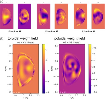
 . The visualization of the prior weight-fields and the resulting PCLLR model weight-field estimate, using $\sigma _g = 0.30$
 , $\theta =2500.0$
 , $n_1=n_2=50$
 , are shown in figure 8. Figure 8(a) illustrates the prior covariance design. Figure 8(b) shows the estimated PCLLR model in physical space. It is possible to use different prior smoothness and different orders, but the final result tends to end up looking similar to what is shown in panel (b), as long as the model selection scheme (4.7) is used to locate the optimal prior strength parameter $\theta$
 in (4.10). Panel (a) will have sharper features for smaller $\sigma _g$
 and more diffuse features for larger $\sigma _g$
 . The cutoff orders have been fixed for simplicity.
(a) Visualization of three random prior draws of the PCLLR $\boldsymbol {\beta }$ parameter using the smoothness enforcing covariance (4.10). (b) Visualization of the estimated PCLLR model in physical space, using the prior shown in panel (a). The inner product of the weight fields in panel (b) with the pair of features for a plasma time-slice (4.8), plus an intercept term, yields the PCLLR model log-odds output, as defined by (4.1).

It is interesting to attempt to interpret the weight-field visualizations in figure 8(b). Recall that these weight fields are applied to a $(1/2)\boldsymbol {J}\boldsymbol {\cdot }\boldsymbol {A}$ feature time slice after subtracting the database mean fields, which are displayed in figure 4. It is clear that the toroidal feature preferentially emphasizes certain edge properties of this differential. It seems plausible that many of the degrees of freedom in the PCLLR model would be spent associating certain classes of plasma shapes (edge geometry) to a hazard value. This is because certain classes of plasmas are more prone to tearing-mode onsets than other classes of plasmas, and these plasmas tend to have different current density distribution support.
It should be understood that the PCLLR model inner product is here split in two terms $\boldsymbol {\beta }^{\rm T}\tilde {\boldsymbol {z}} = \boldsymbol {\beta }_1^{\rm T}\tilde {\boldsymbol {z}}_1 + \boldsymbol {\beta }_2^{\rm T}\tilde {\boldsymbol {z}}_2$ , where the first corresponds to the toroidal basis set and the second corresponds to the poloidal basis set. The two parts are visualized separately as in (4.8), defining the respective weight vectors $\boldsymbol {w}_1$
 and $\boldsymbol {w}_2$
 . The average ratio of the size of the toroidal part of the inner product to both parts across the dataset is $\langle |\boldsymbol {\beta }_1^{\rm T}\tilde {\boldsymbol {z}}_1| / \sqrt { (\boldsymbol {\beta }_1^{\rm T}\tilde {\boldsymbol {z}}_1)^2 + (\boldsymbol {\beta }_2^{\rm T}\tilde {\boldsymbol {z}}_2)^2} \rangle = 0.78$
 . The same average increases to $0.83$
 if only the actual event samples are used. This suggests that the toroidal part of the feature pair is more important with respect to the task.
4.3. Gradient boosting machine (GBM) using principal component feature set
The GBM (Friedman Reference Friedman2001) is here used to represent powerful nonlinear modelling capability to assess how much model performance is lost by being constrained by the linear (but easily visualizable) PCLLR model detailed above. The implementation (Chen & Guestrin Reference Chen and Guestrin2016) is used in what follows. GBMs are known to be among the most efficient techniques in machine learning to model general tabular datasets (Caruana & Niculescu-Mizil Reference Caruana and Niculescu-Mizil2006; Hastie, Tibshirani & Friedman Reference Hastie, Tibshirani and Friedman2009). The dimensionally reduced dataset used in this work arguably falls into this category. Learning the hazard function with a GBM means that the log-odds function (4.1) is replaced by a sum of $B$ sequentially fitted nonlinear function

where $F_0$ is a baseline bias and each additional term $F_i(\boldsymbol {z})$
 is a general regression tree, designed to improve the fitness of the prior sum of $i-1$
 trees. The relationships among the log-odds, the probability and the hazard are unchanged. Unfortunately the ability to specify closed-form (approximate) posterior models, as could be done for the PCLLR, is lost. Also lost is the ability to clearly visualize a unique model weight field. Instead, the GBM model is here evaluated based on the outputs and fitness directly. Standard nested cross-validation is used to estimate these quantities. The GBM is fit to minimize the negative of (4.4), reported by dividing it by the number of samples evaluated (since the test sets differ in size, the per-sample average has to be used). The regularization of the GBM is largely controlled by the number of boosting rounds $B$
 , the depth of the regression trees and the learning rate. Typically, the number of boosting rounds is auto-detected using an inner cross-validation scheme that stops early when the validation set metric starts to increase. In what follows, a few different maximum tree-depths are evaluated, while adjusting the learning-rate such that the per-split optimum number of boosting rounds is in the range $B\approx 500\unicode{x2013}1000$
 .
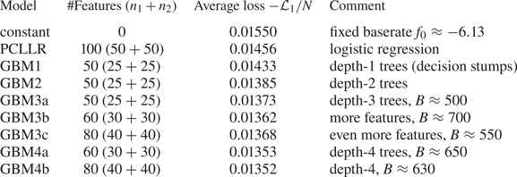
Table 1 shows a comparison of the best achieved loss functions for the different models used in this work. The first row represents the ‘constant’ model, which uses no covariates at all. It is simply the assertion that the baserate applies for all samples in the database. If there are $E$ events and $N$
 examples in the dataset, then the baserate model can be defined by the log-odds value $f_0 = \log [ p_0 / (1-p_0) ]$
 , where $p_0=E/N$
 . The second row shows the PCLLR model using a total of $100$
 features. Notice that the intercept parameter for the PCLLR model is close to the value of $f_0$
 . Notice further that the initial bias in the GBM function (4.11) is taken to be $f_0$
 (for the available training set, the exact value depends on random splits). The remaining the rows in table 1 show loss function results for various GBM settings and using variable PCA truncations.
Comparison of average negative log-likelihood loss function values for a set of GBMs configured by increasing tree depth level. The loss function values should be seen in relation to the PCLLR model, and the improvement obtained with the GBM compared to the PCLLR can be put in context by the difference between the constant model and the PCLLR model.

The difference between the constant model and the PCLLR model is $0.94\times 10^{-3}$ (nats/sample). The difference between the PCLLR model and the GBM3b model is (also) $0.94\times 10^{-3}$
 . This suggests that the improvement (in the data likelihood sense) in going from the PCLLR model to the GBM model is as large as going from no model (just baserate) to the PCLLR model. The next subsection goes into further details on how the model quality improves for the GBM compared to the PCLLR.
4.4. Comparing the calibratedness of the models
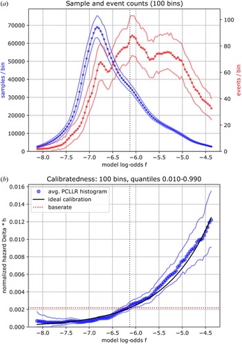
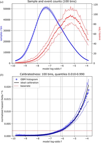
Calibratedness here means that the empirical hazard value, as explained in what follows, should equal its ideal relationship to the model log-odds output $f$ , as given by (4.3). Figure 9 shows a detailed assessment of the calibration of the PCLLR model. Figure 10 shows a detailed assessment of the calibration of one of the GBM models. In panel (a) in both of these plots, the number of samples within a small range of the respective model log-odds output is counted. Both the total number of samples and the number of event samples in each such bin are shown (blue and red, respectively). The total number of samples multiplied by $\varDelta$
 gives the dwell time (the total plasma time) of the dataset in each bin. Panel (b) in both plots shows the ratio of the event count divided by the dwell count. This is the (normalized) empirical hazard (events/sample). Panel (b) also shows the ideal value of $\Delta h$
 as the black solid line. The PCLLR posterior variability of these histogram-based plots is indicated by the uncertain region (pale lines indicate quantiles $0.05$
 , $0.50$
 and $0.95$
 ). For the GBM, the uncertain region is instead derived from the spread among the different complete sets of test set evaluations. The respective ranges of the horizontal axis in the plots are defined by the quantiles $0.01$
 and $0.99$
 of the model output range across the dataset. Going too far out necessarily breaks any comparison to the empirical ratios since the number of samples (and events) will go to zero, making the statistics insufficient for meaningful interpretation.
(a) Histogram counts of the database samples sorted along the output of the PCLLR model. (b) Ratio of the event count divided by the dwell count. This ratio is supposed to be as close as possible to the ideal relationship shown by the black solid line. The PCLLR model calibration is assessed by sampling its posterior parameter and regenerating many histograms. The distribution of the calibrations are shown in the plot: the upper and lower bounding lines represent quantiles $0.95$ and $0.05$
 , respectively.

(a) Histogram counts of the database samples sorted along the output of a GBM model with maximum tree depth $3$ . (b) Ratio of the event count divided by the dwell count. This ratio is supposed to be as close as possible to the ideal relationship shown by the black solid line. The GBM model calibration is assessed by $8$
 -fold splits of the dataset with inner cross-validation. The distribution of the calibrations are shown in the plot. Here the upper and lower bounding lines represent the $0.95$
 and $0.05$
 quantiles, respectively, from the spread across the test set predictions.

The plots clearly show that the (PC-)GBM model has managed to achieve approximate calibration much better than the PCLLR model. For example, the region with peak dwell count in figure 9(a); $f\approx -6.75$ , lies below the reference curve (solid black) in figure 9(b). Presumably, this is because the linear model is not flexible enough to straighten out the fit in that region without being penalized in other parts of the calibration curve. The PCLLR model is above the reference curve around the baseline hazard at $f\approx -6.13$
 . The multi-modal appearance of the event count and the related non-monotonic gradient of the dwell count are other indicators of inadequate modelling. Figure 10(b) in contrast exhibits a more regular closeness to ideal calibration, and achieves this by using a larger range of model outputs (as indicated by the greater span on the horizontal axis). Figure 10(a) also shows a smoother dwell and event count, compared to those in figure 9(a). These calibration plots, combined with table 1, provide strong arguments that the GBM model should be preferred in most cases (the GBM is much harder to visualize and interrogate, so it is beneficial to be analysed in combination with the PCLLR model) since it outputs well calibrated hazard rates across a large portion of the database, using fewer PCA components.
4.5. PCLLR-based comparison to alternative field features
This subsection reports numerical experiments that compare the quality (with respect to the TM onset event) of the $\boldsymbol {J}\boldsymbol {\cdot }\boldsymbol {A}$ field feature to a standard alternative (to be defined below). Two ‘controls’ are also assessed. The first control is a field feature with only geometric information about the support of the current density (in which region it is non-zero). The second control uses the actual $\boldsymbol {J}\boldsymbol {\cdot }\boldsymbol {A}$
 feature but with randomly permuted target labels. The idea with this control is to destroy the association between the feature and the target labels. This establishes a ‘no signal’ floor.
Specifically, the three unique pairs of field features are as follows. First is the physically motivated pair $(f_{{\rm tor}}, f_{{\rm pol}})$ which is a main topic of the present study. Second, as the standard comparison, a direct mapping of the EFIT polynomials to axisymmetric space is used. This pair is $(J_{\phi }, \delta B_{\phi })$
 , where $\delta B_{\phi }$
 is the plasma current generated toroidal magnetic field (mapping the so-called poloidal current function). This feature pair is essentially (differing by factors $-1$
 , $r$
 and $\mu _0$
 ) the source term for the $\boldsymbol {A}$
 field calculations via (3.6) and (3.7). The third feature pair has no information about the values of the current density. The pair of fields used for this control is the indicator, or ‘mask’, function for $J_{\phi }$
 and the same mask function multiplied by $1/r$
 . The mask takes the value $1$
 for $(r,z)$
 inside the last closed fluxed surface, and $0$
 otherwise. It is expected that this third feature should carry significantly less information about the TM events than the other two features. The PCA dimensionality reduction machinery detailed in § 3.1 is applied independently to these alternative feature pairs. Each feature set has the same dimensionality (two different sets of scalar values on a $65$
 -by-$65$
 grid).
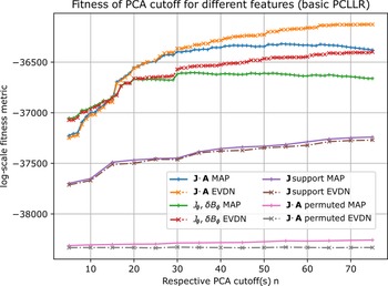
For each of the above three sets of features (and the fourth no-signal control), a basic PCLLR model is fitted with an optimal diagonal regularizer, for a range of PCA cutoffs $n=n_1=n_2$ . This is done for both types of evidence scores (see § 4.1): (i) evaluation of $\mathcal {L}_1+\mathcal {L}_2$
 and (ii) evaluation of $\mathcal {L}_1+\mathcal {L}_2+\mathcal {L}_3$
 . The results are shown in figure 11. In the figure, metric (i) is denoted MAP (maximum a posteriori), and metric (ii) is denoted by EVDN (evidence). The dashed lines with angled cross-markers show the MAP metric for the respective feature set. The solid lines with straight cross-markers show the EVDN metric for the respective feature set.
Comparison of different sets of field features using a basic PCLLR model selection framework. The dashed lines (with angled cross-markers) show the MAP score and the solid lines (with straight cross-markers) show the EVDN score for each respective feature set. The bottom traces are obtained by randomly shuffling the target labels so that there should be no information about the target in the (any) feature. The indicator feature (‘$\boldsymbol {J}$ support’, see main text) provides some fitting power, but much less so than for the $(J_{\phi }, \delta B_{\phi })$
 and $(f_{{\rm tor}}, f_{{\rm pol}})$
 features. The highest evidence scores are obtained with the $\boldsymbol {J}\boldsymbol {\cdot }\boldsymbol {A}$
 based field feature. It is also seen that a PCA cutoff at $n\sim 50$
 is suggested by the MAP score, whereas the EVDN score flattens out at a higher cutoff $n\sim 75$
 .

It can be observed that the $\boldsymbol {J}\boldsymbol {\cdot }\boldsymbol {A}$ based field feature does attain higher MAP and EVDN scores (for $n > 15$
 ) than does the standard mapped EFIT field feature $(J_{\phi }, \delta B_{\phi })$
 . For aggressive PCA cutoffs ($n < 15$
 ), the opposite ordering is seen (green and red traces are above the blue and orange traces). The MAP scores suggest that $n\sim 50$
 is a good PCA cutoff, whereas the EVDN scores seem to suggest that it is justified to go higher to $n\sim 75$
 . It is important to remember these are heuristics for the PCLLR model, and that the PCLLR model itself is much less efficient than the nonlinear GBM. There is nothing exact about such suggested cutoffs. The point of figure 11 is to compare the $\boldsymbol {J}\boldsymbol {\cdot }\boldsymbol {A}$
 field feature to a possible standard alternative, using the computationally efficient PCLLR evidence scores.
The two controls show the expected behaviour. The indicator feature with no access to continuous values from the EFIT (only the current density support and the inverse radial coordinate information) is graded far below the other two features with further information. The no-signal floor value can be defined by the experiments evaluated with randomly permuted target labels. There should be no added value of using more PCA components in this case and flat traces independent of $n$ are expected and obtained.
These calculations provide evidence that the (more involved, but physically motivated) $\boldsymbol {J}\boldsymbol {\cdot }\boldsymbol {A}$ field feature does have some informational advantage, with respect to the TM onset event, over what is arguably a direct/native EFIT axisymmetric field feature, in the context of this study.
5. Example applications
This section demonstrates two applications of the statistical TM onset hazard function developed in the previous section. Specifically, the GBM function is used as it is well calibrated and much more accurate than the PCLLR alternative. The first application is the pointwise evaluation of the hazard function along time in two example DIII-D discharges. The second application is the visualization of an apparent database-wide observational trade-off in plasma performance versus the TM onset rate. The use of a hazard function as a conditional generator of probabilities can be found in Appendix B, providing additional clarification of and motivation for these examples.
5.1. Hazard ratio time trace monitoring
A well-calibrated and sufficiently accurate (according to some criteria yet to be defined) hazard function could, in principle, be used to monitor the instantaneous risk for TM onset in a plasma in real time. Knowing the main effects of control actuators on the (future) hazard value may then allow regulation to actively lower the risk in the event that some unforeseen perturbation has put the tokamak plasma in a state of elevated TM hazard. This type of reasoning is sometimes known as ‘proximity control’ and is an active research topic at DIII-D (Barr et al. Reference Barr, Sammuli, Humphreys, Olofsson, Du, Rea, Wehner, Boyer, Eidietis and Granetz2021). A reactor grade tokamak cannot maintain operation in a plasma state where a truthful hazard function returns a value comparable to the inverse discharge time. Control of the actuation effect on the hazard function adds another layer of complexity in that a model of the future feature state based on the actuation programming is required, which is beyond the scope of this work. Further details on these types of applications of a hazard function are found in Appendix B.
To assess the capability of the estimated hazard function in this work for this type of application, the time-traces for specific experiments can be calculated after-the-fact. For this purpose, it is convenient to introduce the non-dimensional hazard ratio

where the denominator is defined as the baseline hazard $\hat {h}_0$ , which is expressed in terms of the total number of events $E$
 and total number of samples $N$
 across the database by

with the last relation due to $E \ll N$ . A hazard ratio of $1$
 means that the expected rate of onset at the present time instance is equal to the global database average rate. A hazard ratio below $1$
 means that the present time instance is less prone to TM onset compared to the average rate. A hazard ratio of $2$
 , for example, means that the TM onset rate is elevated by a factor of $2$
 . And so on.
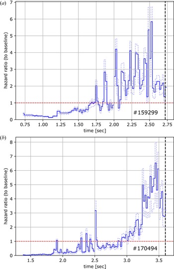
Figure 12(a,b) shows the time-traces of the predicted hazard ratios (5.1) for the same example DIII-D experiments that were used in figure 1(a,b). The probability of TM onset over a segment in time is determined by the integral of the hazard (known as the cumulative hazard). A short spike of moderately elevated hazard (perhaps due to an unusually perturbed equilibrium reconstruction) does not matter much for the probabilistic model. Sustained levels of high hazard are what generate a high probability of TM onset, according to the model. The baseline rate, $H=1$ in the plots, roughly corresponds to one TM onset every 10 s (database wide average). Here, $H=5$
 approximately implies one onset every 2 s. It is critical to realize that these rates are to be interpreted in the sense of an exponential distribution. Specifically, if the instantaneous hazard is $0.5\,\mathrm {s}^{-1}$
 , assuming the plasma is in a steady-state where this value is maintained constant, then the expected time until a TM onset is $2.0\,\mathrm {s}$
 . However, the standard deviation of that random time is also $2.0\,\mathrm {s}$
 . This is a property of the exponential distribution; the ratio of its standard deviation to its mean is one (its coefficient of variation). Keeping this in mind is essential when interpreting the hazard (ratio) values in relation to events that happened, seemed like they should have happened or seemed like they should not have happened. The hazard model accommodates all these cases flexibly. Only an extremely high value of the instantaneous hazard is akin to a committed statement that ‘a TM event will happen here and now’.
Example time-traces of the hazard ratio $H$ (5.1). Here, $H(t)=1$
 means that the instantaneous TM onset rate is deemed to be $h(t)\approx 0.10\,\mathrm {s}^{-1}$
 . (a,b) Time-traces corresponding to the respective panels in figure 1. In both these cases, a sustained elevated hazard ratio is predicted well before the actual events happen (RM onsets in both cases). The (terminating) dashed vertical line in panel (a) corresponds to the RM signal detection at the $4.0\,\mathrm {G}$
 threshold in figure 1(a). Similarly the terminating dashed vertical line in panel (b) corresponds to the RM signal detection in figure 1(b). Both of these discharges eventually develop LMs.

Note that the only information used for the predictions demonstrated in figure 12(a,b) are the magnetics only equilibrium reconstructions. So all the trends in these plots must be due to trends in these reconstructions. The indicated range of predictions (pale blue lines) indicate the first and third quartiles of the ensemble of predictions, obtained using an $8$ -fold outer test set evaluation, repeated $100$
 times. The GBM model was used for the predictions.
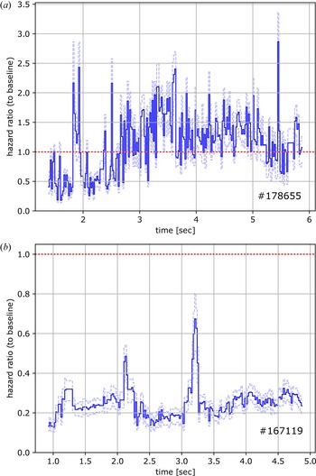
Figure 13(a,b) shows example DIII-D discharges that do not develop any TM event. Panel (a) shows the evaluation of the hazard ratio across an instance of a class of plasmas known to be highly prone to disruptive TM onset events. The hazard ratio is sustained above the baseline rate across a large fraction of the current flat-top. It seems that an event could have happened in this discharge. Panel (b) is an evaluation across a low-powered discharge that appears to be several times less prone to TM onset events compared to the baseline rate. Taken together, the examples displayed in figures 12 and 13 appear to present a strong case for the usefulness of the hazard function for time-slice risk assessment.
Example time-traces of the hazard ratio $H$ (5.1). In contrast to the discharges shown in figure 12, these two discharges did not experience any detected ($|n|=1$
 ) TM event throughout. The discharge in panel (a) is of a type known to have many disruptive TM events. The discharge in panel (b) is low-powered and is rated as very TM stable by the hazard ratio predictions. The discharge in panel (a) has significant sawtooth activity (odd RM trace signal) starting around $t\approx 2.0\,\mathrm {s}$
 and it does experience a $|n|=2$
 TM onset (rotating) at $t\approx 2.4\,\mathrm {s}$
 .

5.2. Plasma performance versus TM onset hazard ratio
The performance of a tokamak plasma can be measured in many ways. One useful metric is the ratio

where $\langle p\rangle _V$ is the volume averaged plasma pressure, $\tau _E$
 is the energy confinement time, $I_p$
 the plasma current, $a$
 the plasma minor radius and $B_T$
 the toroidal magnetic field (Paz-Soldan Reference Paz-Soldan2021). The product of the pressure and the confinement time is a proxy for fusion power, and the denominator is a penalty for inefficiency (proxy for the cost of the configuration).
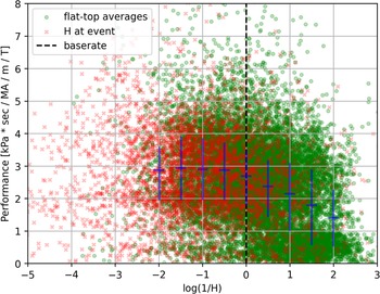
Figure 14 has metric (5.3) on the vertical axis and $-\log H$ , from (5.1), on the horizontal axis. For the green markers, the flat-top averaged quantities are used exclusively. Green markers indicate single DIII-D experiments (whether it experiences an onset event or not). The performance increases in the up direction in the plot. Therefore, the most desired region is the upper-right region (low TM risk, high performance). The standard confinement time estimate in the DIII-D database is quite volatile, which may explain some of the scatter in the vertical direction.
Flat-top average plasma performance is shown on the vertical axis. The negative logarithm of the flat-top average (green markers) hazard ratio prediction is shown on the horizontal axis. The mean and quartile range for thin vertical slices of the scattered data (for green markers) are marked by the blue line segments. The most desirable operating point is the upper-right region, with high performance and low modelled rate of tearing onset events. Even in this simple plot (see text for discussion), an intuitive database-wide trend can be observed; higher performing shots tend to have higher rates of TM onset. Actual TM events are shown as red markers at the hazard ratio value, at the time of the event.

The blue vertical line segments connect the first and third quartiles of the distribution of the green markers at a thin range of hazard ratios (horizontal axis range). The mean value of this distribution is shown by the short blue horizontal line segment. This short line segment also indicates the range of hazard ratios used for these statistics. Note that here the time-variation of the hazard ratio (see previous application example) is collapsed into a single average value, which would tend to blend events and non-events. Additional blending of the performance axis is likely due to the non-equivalence of current and pressure flat-top intervals. Ideally the specific averaging intervals for the performance should, in general, not be from the start of the current flat-top. However, the trend shown by the localized blue quartile range (vertical line segment) and localized mean value (horizontal line segment) indicators is still clear. The DIII-D database operational space exhibits an observational tendency to higher TM onset rates for the higher performance discharges (up to some saturation level where the TM risk may be debilitating and operation becomes inaccessible). The purpose here is not a detailed analysis of this particular operational space as that would require much refined production of this plot. Rather the quantification of this intuitive trend using the machine-learned hazard function suggests its usefulness in tokamak data analysis.
The red markers are located at the average performance metric operating point but their hazard ratio coordinate is not the mean for the plasma but its value at the timestamp of the event. A red marker is only added for plasmas that did experience a TM onset event. It is clear that the final hazard value at the time of the event generally is higher (as can be understood by the time traces in the previous application example) and that many event locations in this space are dangerously far (to the left in the plot) away from mean values.
6. Discussion
This study combines many elements of tokamak database analysis and improvements can be envisioned at every stage in its pipeline. In what follows, a set of limitations will be listed, combined with ideas for possible improvements. This section ends with a brief concluding paragraph.
Compared to earlier work, the inclusion of both LM and RM detectors is a critical improvement, allowing the approximation of more complete statistics on TM onsets and hence to learn a useful hazard function. Nevertheless, the RM and LM detectors would benefit from further analysis to identify possibly systematic fault modes. The threshold values were fixed in this work, set to reasonable levels, as discussed in § 2.3. Sensitivity studies driven by variations of these thresholds could be useful to increase confidence in the statistical regularity of the results, but such studies would carry a high computational cost (and seem unlikely to matter greatly). Probably more important is to check specifically the RM detector, which is suspected to experience cross-talk between its odd–even categorization in some cases. More advanced RM analyses are possible (Hole & Appel Reference Hole and Appel2007; Olofsson et al. Reference Olofsson, Hanson, Shiraki, Volpe, Humphreys, Haye, Lanctot, Strait, Welander and Kolemen2014) and would be worth the additional effort required if the quality of labelling can be shown to improve significantly. Although not done here, it is straightforward to extend the machine learning formulation to model the expected flavour of TM onset, RM or LM, in addition to the total hazard. That might be useful in some applications, but without explicit information about plasma rotation in the features, this type of onset event sub-classification seems ill-posed.
One limitation of the PCA in this work is that the toroidal and poloidal feature fields are analysed and reduced independently. This is a simplification which makes the implementation easier. However, in principle, there should be a joint reduction of these features into a single latent space vector. A natural way to handle this, still using standard numerical linear algebra, is to employ canonical correlation analysis (CCA) of the pair of toroidal and poloidal feature vectors. Other alternatives for dimensionality reduction include non-negative matrix factorization (Hastie et al. Reference Hastie, Tibshirani and Friedman2009), and so-called ‘robust’ PCA (Candès et al. Reference Candès, Li, Ma and Wright2011). Both these alternatives use sparsity promoting optimization techniques, in contrast to classical PCA (and CCA).
The GBM modelling approach has been used for its simplicity and efficiency. It might be possible to improve the modelling further using neural network (NN) structured models. Convolutional NNs could operate directly on the feature fields as image processing systems; however, it is unclear if there is enough information in the standard magnetics-only equilibrium reconstructions to justify such a brute-force approach.
One of the largest limitations of the study is arguably the exclusive usage of magnetics-only equilibrium reconstructions. The internal details of the current density are not well resolved. It is also generally accepted that these reconstructions do not provide high-resolution details of the edge current density. This prevents physics conclusions about detailed onset conditions to be drawn. At this time, there is no DIII-D database-wide coverage of a high fidelity kinetic equilibrium reconstruction constrained by internal diagnostics. This is expected to change in the future and the analysis presented here can then be refined. The limitation to magnetics-only features should be regarded as a necessary first step to establish the fundamental toolkit and its basic performance.
In conclusion, this study shows the development and testing of a suite of analysis tools, capable of associating the calibrated observational rate of TM onset to reconstructed axisymmetric equilibrium field quantities, across a large portion of the available DIII-D dataset. The event signal is derived from non-trivial processing of large amounts of non-axisymmetric magnetics fluctuation diagnostics data. Standard model selection machinery, applied to this particular statistical modelling problem, suggests that the energy-density feature gives a better model compared to the native source term from the equilibrium reconstruction. The toolset was demonstrated in multiple types of machine-learning enabled analyses. Many improvements can be envisioned.
Acknowledgements
The authors thank T. Strait, S. Munaretto and L. Bardóczi for help with the DIII-D magnetics diagnostics.
Editor William Dorland thanks the referees for their advice in evaluating this article.
Funding
This work was supported in part by the U.S. Department of Energy, Office of Science, Office of Fusion Energy Sciences, using the DIII-D National Fusion Facility, a DOE Office of Science user facility, under Award Nos. DE-FC02-04ER54698 and DE-SC0022031.
Declaration of interests
The authors report no conflict of interest.
Disclaimer
This report was prepared as an account of work sponsored by an agency of the United States Government. Neither the United States Government nor any agency thereof, nor any of their employees, makes any warranty, express or implied, or assumes any legal liability or responsibility for the accuracy, completeness or usefulness of any information, apparatus, product or process disclosed, or represents that its use would not infringe privately owned rights. Reference herein to any specific commercial product, process or service by trade name, trademark, manufacturer or otherwise, does not necessarily constitute or imply its endorsement, recommendation or favouring by the United States Government or any agency thereof. The views and opinions of authors expressed herein do not necessarily state or reflect those of the United States Government or any agency thereof.
Appendix A
Because of the assumption of the Coulomb gauge, $\boldsymbol {\nabla }\boldsymbol {\cdot }\boldsymbol {A}=0$ , the vector potential $\boldsymbol {A}$
 is now also a solenoidal field, and thereby can be expressed in terms of a stream function $\varPhi \equiv r\varTheta$
 as follows:

where $\phi$ is the usual toroidal coordinate and $\psi$
 is the flux function from above. This is a dimensional augmentation of the usual description of the magnetic field in terms of a stream function $\psi$
 : $\boldsymbol {B}=\boldsymbol {\nabla }\psi \times \boldsymbol {\nabla }\phi + rB_{\phi }\boldsymbol {\nabla }\phi$
 . The parallel construction, given by (A1), then provides the following analogues: $\varPhi :\psi$
 , $\varTheta :A_{\phi }$
 and $B_{\phi }:\mu _0 J_{\phi }$
 (note the expressions on the left side have units that carry an extra factor of length compared to the expression on the right.)
Taking the curl of (A1) gives the usual poloidal component of the magnetic field in terms of the flux function $\psi$ : $\boldsymbol {B}_p=({1}/{r})\boldsymbol {\nabla }\psi \times \hat {\phi }$
 as well as a new second-order equation analogous to (3.7):

which can be recast as

where Ampére's law was used for the right-hand-side.
Appendix B
In this Appendix, it is demonstrated how a truthful hazard function can be used in the context of proximity control. Making this link explicit strengthens both the general motivation for an event hazard function and the specific motivation of the hazard monitoring application example in the main text of the paper.
Since the single time-step survival (no event) probability is $\exp (-\Delta h)$ , it follows that the survival probability for multiple time-steps $n$
 is

where $N$ is a stochastic event step index. This is a uniform discretization of the continuous-time analogue (stochastic event time $T$
 )

where, according to the present model, $h(t) = h(\boldsymbol {x}(t))$ (the time dependence of the hazard is due to the time evolution of the state $\boldsymbol {x}$
 ). In this context, time $t$
 is relative to the present time, meaning $t=0$
 is ‘now’ and $t>0$
 is in the future. From (B2), it is now clear how the hazard model $h(\cdot )$
 can be combined with another model $\boldsymbol {f}(\boldsymbol {\cdot })$
 that dictates the evolution of the state variable. With model $\boldsymbol {f}$
 , the state evolution can be written $\dot {\boldsymbol {x}} = \boldsymbol {f}(\boldsymbol {x}, \boldsymbol {u})$
 , where $\boldsymbol {u}(t)$
 is the trajectory of actuators. Therefore, $h$
 and $\boldsymbol {f}$
 together comprise a device that allows the calculation of future survival probabilities $\mathrm {Pr}( T \geq t \,|\, \boldsymbol {x}(0), \boldsymbol {u}(\tau ) )$
 conditioned on future actuator trajectories ($0 \leq \tau \leq t$
 ) and the current state. This type of ‘decoupled’ probability model is by construction applicable in the context of proximity control. The conditional future probabilities can be used in various ways (for example, used as weights on a performance metric in receding-horizon feedback control), but the main points are (i) to detect trajectories that rapidly increase the cumulative hazard $\int _0^t \mathrm {d}\tau h(\tau )$
 and (ii) ability to parametrize future trajectories by control actuation.
The decoupling of the survival (or event) probability, as explained above, is not typically done in tokamak prediction problems. The following thought experiment illustrates a problem that can arise. Suppose an ML model is trained on available observational data to give the probability of tearing occurring within $200\,\mathrm {ms}$ into the future, given the present state (the finite time survival is one minus this probability). Suppose further that the ML model is deployed in the experiment to initiate some (effective) action when the survival probability is deemed too low. In the long run, the original ML model that the feedback decision is based on will become statistically invalid under the new distribution it generates (since the state-to-future-event association has been modified).
The issue is that the future survival depends on the current state and the future actuator programming jointly, and $200\,\mathrm {ms}$ is long enough that future actions matter. Using a state-dependent hazard function as a probability generator is one way to account for these dependencies. Deploying a system that takes action based on the hazard function does not make the same hazard function statistically invalid.