

1. Introduction
Globalization, population growth, and other factors have increased the likelihood for the occurrence of epidemics and pandemics [Engel and Ziegler (Reference Engel and Ziegler2020)], with COVID-19 being the most recent example. A severe pandemic is just one of several low-probability, high-impact events which may lead to a sudden increase in mortality rates, a so-called mortality shock. Mortality shocks lead to changes in mortality data, which in turn can influence model parameters and forecasts [Schnürch et al. (Reference Schnürch, Kleinow, Korn and Wagner2022)]. This is relevant for many applications, including the pricing of mortality catastrophe bonds as well as risk management and reserving decisions in life insurance companies.
A central question with respect to mortality shocks is if and how to treat them in mortality models, regarding both their appearance in past data to which models are calibrated and the possibility of their appearance in future observations. We especially focus on the popular stochastic mortality model by Lee and Carter (Reference Lee and Carter1992, LC). Forecasts under this model are usually obtained by a random walk with drift, which corresponds to a normal distribution assumption. As we demonstrate, mortality shocks can lead to violations of this assumption with potential consequences for forecasts and the quantification of their uncertainty.
One way of addressing this is to suitably adjust the data by outlier adjustment methods. However, depending on the application, it might be questionable to remove genuine observations of extreme mortality from the data. Under the Solvency II framework, for example, solvency capital requirements are calculated as a value-at-risk, for which a realistic evaluation of tail behavior is vital. Moreover, since the COVID-19 pandemic is by now expected to influence mortality data of at least two years (2020 and 2021), exclusion of extreme data would lead to quite a lot of recent information not entering model calibration.
Therefore, it could be more reasonable to not (only) change the data but to change the model by deviating from the normal distribution assumption. This can be done in a generic way, switching to another distribution family with heavier upper tail. Here, we propose and investigate the lognormal distribution. Alternatively, it is possible to explicitly model the occurrence of extreme mortality events, for which we present three approaches (“shock models”) from the literature: a mixture distribution based on the peaks-over-threshold method, a discrete jump diffusion and a regime switching model. They have different theoretical properties and all of them can be useful for describing historical data, but empirically we find the mixture distribution to be most appropriate with respect to several criteria.
Our main contribution to the literature is twofold:
• We propose an adjusted calibration procedure for the shock models, using long-term data to fit the shock parameters and short-term data to fit the remaining parameters, and demonstrate that it clearly improves backtest performance.
• We conduct an extensive empirical evaluation of the different modeling approaches with respect to quality of fit, forecasting performance, and differences in predicted period effects as well as term assurance and annuity values. We introduce five exemplary scenarios for the further development of pandemic-related mortality and show how the models would perform under these scenarios.
Our empirical evaluations take place on an updated version of the data set used by Schnürch et al. (Reference Schnürch, Kleinow, Korn and Wagner2022) and we refer to this paper for a more detailed description of the data and notation. We get yearly death rates $m_{x, t}^i$ directly from the Human Mortality Database (2021). For years in which these are unavailable yet, we calculate them from weekly death counts obtained from Short Term Mortality Fluctuations (2021). Here, we denote age by $x\in {\cal X} = \{ x_1,\; \ldots ,\; x_A\}$
 and consider 5-year age groups so that x 1 = 35 − 39, x 2 = 40 − 44, …, x A = 90 +. The population is denoted by $i\in {\cal P}\, \colon = \{ 1,\; 2,\; \ldots ,\; P\}$
 with P = 27 as we consider the male, female, and total populations of 9 European countries.Footnote 1 The availability of years depends on the country, which we usually ignore in our notation and simply denote the calendar year by $t\in {\cal T}\, \colon = \{ t_1,\; \ldots ,\; t_Y\}$
 .
We proceed as follows: section 2 introduces the LC model along with different ways of forecasting its period effect. For the approaches explicitly modeling the possibility of mortality shocks, we describe a new, adjusted calibration procedure. In section 3 we present empirical results on the normal distribution assumption for the period effect increments and evaluations of the models with respect to quality of fit, forecasts, and forecasting performance in a backtest and under different future scenarios. Section 4 concludes.
2. Methodology
2.1. The Lee–Carter model
Lee and Carter (Reference Lee and Carter1992) model logarithmic death rates for a life aged x in year t belonging to population i as

with age-specific base mortality level $\alpha _x^i$ , period effect $\kappa _t^i$
 related to the general development over time, and age effect $\beta _x^i$
 describing the impact of this development on different ages. The error terms $\varepsilon _{x, t}^i$
 are assumed to be independent, homoskedastic, and normally distributed. In the following, we suppress the dependence on the population i in our notation.
The model (1) is calibrated via singular value decomposition. The constraints

are imposed to make its parameters identifiable. Forecasts of future mortality rates are obtained by choosing a suitable model for the estimated period effects $( \hat {\kappa }_t) _{t\in {\cal T}}$ , usually for their first differences $\Delta \hat {\kappa }_t\, \colon = \hat {\kappa }_t - \hat {\kappa }_{t-1}$
 .
The choice of such a time series model depends on its compatibility with observed data but also on the expectations and preferences of the modeler. In the following, we present several possibilities for this choice. An overview is given in Table 1.
Overview of the different modeling approaches for $\hat {\kappa }_t$

2.2. Forecasting the period effect with an ARIMA model
The simplest and most often used approach is to model $( \hat {\kappa }_t) _{t\in {\cal T}}$ as a random walk with drift (RWD), i.e.,

This yields explicit formulae for both point and interval forecasts of the period effect, which are then inserted into (1) to obtain death rate forecasts. We refer to Schnürch et al. (Reference Schnürch, Kleinow, Korn and Wagner2022), who provide details on the procedure and demonstrate that a mortality shock in the forecast jump-off year influences RWD point forecasts and a mortality shock at any time in the calibration data set influences interval forecasts.
Although the RWD has been demonstrated to work quite well in the literature [Lee and Carter (Reference Lee and Carter1992); Tuljapurkar et al. (Reference Tuljapurkar, Li and Boe2000)], it has a few drawbacks, for example, its strong dependence on $\hat {\kappa }_{t_Y}$ , the period effect in the jump-off year. A natural idea is to replace the RWD by a general autoregressive integrated moving average (ARIMA) model, which potentially places less weight on the last period effect and also yields a better fit. ARIMA models have three hyperparameters, the autoregressive order p, the order of integration d, and the moving average order q, which we choose by the auto.arima algorithm: for each population, we consider all ARIMA(p, d, q) process specifications with p ≤ 5, d ≤ 1 and q ≤ 5 and select the one which strikes the best balance between low calibration error and parsimony. We refer to Hyndman and Khandakar (Reference Hyndman and Khandakar2008, Section 3) for a detailed description of the algorithm as well as the R [R Core Team (2019)] implementation we use. Similarly as for an RWD, a mortality shock in the calibration data set of an ARIMA(p, d, q) model will persist in its forecasts if p > 0 or d > 0, which is the case for all ARIMA models the auto.arima algorithm has returned in our numerical experiments.
2.3. Dealing with mortality shocks in an ARIMA setting
In this section, we describe six alternative methods to explicitly deal with outliers in the period effect.
One way of addressing the occurrence of mortality shocks is to reduce or completely remove their effect on calibration, so that the model is trained with a focus on “normal” data. Therefore, it should only be used to make forecasts conditional on the assumption that no major mortality shocks will occur in the future or if the possibility of such shocks is not relevant for the considered application.
Replacing by a best estimate
The most radical way of reducing the effect of mortality shocks on model calibration is to exclude years in which they occur from the data, which has a similar effect as replacing the observations in these years by best estimates based on shock-free data. For the example of COVID-19, we calibrate an LC model on data up to 2019, obtain forecasts for 2020 by an RWD and recalibrate the model on the data including these 2020 forecasts. This approach has been investigated and compared to the RWD without data exclusion by Schnürch et al. (Reference Schnürch, Kleinow, Korn and Wagner2022). It obviously prevents the excluded mortality shock from influencing mortality forecasts in any way.
Intervention model
Alternatively, one can apply an intervention model to the period effect time series, as Lee and Carter (Reference Lee and Carter1992) have done to diminish the influence of the 1918 pandemic. This means that a binary dummy is added to the RWD model (3), yielding

where $t^{\rm out}\, \colon = {\rm argmax}_{t = t_2, \ldots , t_Y} \Delta \hat {\kappa }_t$ is the year with the largest (upward) mortality shock and the maximum likelihood estimate for φ is $\Delta \hat {\kappa }_{t^{\rm out}} - \hat {\mu }$
 . For the calibration period t ∈ {1991, …, 2020}, we usually get t out = 2020 so that the parameter φ absorbs the mortality shock induced by the COVID-19 pandemic. Therefore, this intervention model can be expected to behave very similarly to our best estimate approach which directly ignores 2020. In particular, it only allows the mortality shock to influence forecasts via the α x and β x parameters, which are calibrated on the original data including the shock. However, changes in these parameters in response to a COVID-19-type shock are expected to be small [Schnürch et al. (Reference Schnürch, Kleinow, Korn and Wagner2022), Proposition 1].
More sophisticated methods are available, including more general intervention models [Box and Tiao (Reference Box and Tiao1975)] or techniques from time series outlier detection and adjustment [Li and Chan (Reference Li and Chan2005, Reference Li and Chan2007)]. However, we restrict our attention to the best estimate replacement and the simple intervention model (4) as we deem these sufficient to illustrate the consequences of excluding mortality shocks from the model calibration.
Another way of dealing with mortality shocks is to include them in the calibration data and adapt the model accordingly. More precisely, we adjust the distribution assumption.
Lognormal distribution
A natural idea is to simply replace the normal distribution ${\cal N}( 0,\; \sigma ^2)$ in (3) by some asymmetric, unimodal distribution with heavier upper tail. There are several distributions with this property in the literature. We choose the lognormal distribution, which is known to be suitable for a lot of applications in finance such as modeling stock prices or interest rates.
As the lognormal distribution is only supported on the positive real line and $\Delta \hat {\kappa }_t$ is usually negative for many t, some data transformation is necessary. We apply

with λ > 0. The entire approach is equivalent to a Box–Cox transformation [Box and Cox (Reference Box and Cox1964)] with non-zero shift parameter $\left \vert \min \limits _{\tilde {t} = t_2, \ldots , t_Y} \Delta \hat {\kappa }_{\tilde {t}} \right \vert + \lambda$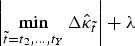 .
We calibrate λ along with the two parameters of the lognormal distribution by maximum likelihood estimation. With the calibrated model, we perform Monte Carlo simulation (with 104 paths) and apply the inverse of (5) to obtain period effect increment forecasts, which are then converted into death rate forecasts. As the forecast for $\hat {\kappa }_{t_Y + 1}$ is based on the unmodified value of $\hat {\kappa }_{t_Y}$
 , a shock to the period effect in the jump-off year will persist in forecasts.
Of course, it is also possible to change the distribution assumption so as to explicitly account for mortality shocks. We consider three methods from the literature, which are all based on the idea that there are two different underlying states governing mortality, a normal state and a shock state. This idea is implemented more or less directly.
Peaks-over-threshold
Chen and Cummins (Reference Chen and Cummins2010) propose to apply the peaks-over-threshold (POT) method from extreme value theory to the first differenced period effect $\Delta \hat {\kappa }_t$ , assuming that it follows a two-component mixture distribution. More precisely, a threshold $u\in \mathbb{R}$
 is specified below which $\Delta \hat {\kappa }_t$
 is modeled by a normal distribution, whereas it is modeled by a generalized Pareto distribution (GPD) above this threshold. We denote this by

where G(ξ, ζ) is a GPD with shape parameter $\xi \in \mathbb{R}$ and scaling parameter ζ > 0. The period effect follows an RWD during normal times, but the model allows for the fact that shocks can occur and lead to non-normal behavior by approximating the upper tail of the distribution with a GPD. This is justified by the Pickands–Balkema–de Haan theorem from extreme value theory [Balkema and de Haan (Reference Balkema and de Haan1974); Pickands (Reference Pickands1975)]. Similar mixture models have been successfully applied both on synthetic [Mendes and Lopes (Reference Mendes and Lopes2004)] and on real data [stock index returns, Behrens et al. (Reference Behrens, Lopes and Gamerman2004)].
A critical aspect of this method is the choice of the threshold u, which should not be too large so that the GPD parameters are calibrated on sufficiently many observations, but it should also not be too small so that only a minor share of the observations falls in the non-normal part of the distribution. Many procedures to estimate the threshold have been proposed in the literature [Scarrott and MacDonald (Reference Scarrott and MacDonald2012)]. Here, we follow Chen and Cummins (Reference Chen and Cummins2010); Mendes and Lopes (Reference Mendes and Lopes2004) and calculate the profile likelihood

where ${\cal L}$ denotes the likelihood function of model (6). We try all values $u \in \{ q_{85}( \Delta \hat {\kappa }_t) ,\; q_{86}( \Delta \hat {\kappa }_t) ,\; \ldots ,\; q_{95}( \Delta \hat {\kappa }_t) \}$
 , where $q_z( \Delta \hat {\kappa }_t)$
 denotes the empirical $z\%$
 quantile of $\Delta \hat {\kappa }_t$
 , and we choose u to maximize ${\cal L}_p( u)$
 . Then, we calibrate the parameters μ, σ, ξ, and ζ conditionally on the fixed u by penalized maximum likelihood estimation. The likelihood is penalized as proposed by Coles and Dixon (Reference Coles and Dixon1999) in order to stabilize the calibration.Footnote 2 We refer to Chen and Cummins (Reference Chen and Cummins2010) and section 2.4 below for further details on the calibration algorithm. Chen and Cummins (Reference Chen and Cummins2010) also describe how to simulate from their model, which we use to obtain point and interval death rate forecasts by Monte Carlo simulation (with 106 paths). In particular, analogously to the lognormal distribution approach, forecasts for $\hat {\kappa }_{t_Y + 1}$
 are based on the unmodified value of $\hat {\kappa }_{t_Y}$
 and a shock to the period effect in the jump-off year t Y will persist in forecasts.
Jump model
Another possibility to account for shocks is to allow for transitory mortality jumps. Several applications of jumps have been investigated in the literature both on discrete-time and continuous-time mortality models, see Regis and Jevtić (Reference Regis and Jevtić2022) for a recent overview, which also includes multi-population models. Here, we follow Chen and Cox (Reference Chen and Cox2009), who propose

where $e_t\sim {\cal N}( \mu ,\; \sigma ^2)$ i.i.d., the jump severities W t follow i.i.d. ${\cal N}( m,\; s^2)$
 distributions and N t are i.i.d. Bernoulli random variables with jump probability p ∈ (0, 1), i.e., N t = 1 means there is a jump in mortality at time t and N t = 0 means there is none. Independence is assumed between e t, W t, and N t. It is easy to see that $\hat {\kappa }_t$
 follows an RWD as long as there is no jump and that it returns to this RWD after a jump has taken place, unless N t = N t−1 = 1. This latter case corresponds to two consecutive jumps or one longer-lasting jump and by (8) leads to an increase in volatility of $\Delta \hat {\kappa }_t$
 from $\sqrt {\sigma ^2 + s^2}$
 to $\sqrt {\sigma ^2 + 2s^2}$
 .
Although it is possible for longer-lasting shocks to occur under the jump model, its conceptual idea is to model transitory shock events which only influence mortality for one time period (one year). In particular, we refrain from modeling a serial correlation of N t, i.e., a non-trivial dependence structure of shock occurrence over time.
In contrast to the POT model, we do not only consider the possibility of upward jumps here, as we allow m ≤ 0. However, we expect that m > 0 for most populations because transitory mortality jumps usually move in an upward direction, whereas mortality improvements often play out over a longer time period.
The model is calibrated by conditional maximum likelihood estimation as described by Chen and Cox (Reference Chen and Cox2009). Point and interval forecasts are obtained via Monte Carlo simulation (with J = 106 paths) from (8). Estimates for the realized values of the unobservable $W_{t_Y}$ and $N_{t_Y}$
 must be available in order to obtain the first forecast $\hat {\kappa }_{t_Y + 1}$
 . We propose the following approach to calculate these estimates: Set $N_{t_Y}^a\, \colon = 1$
 and

on Monte Carlo paths a = 1, …, πJ, where

and πJ is rounded to the nearest integer. On the remaining Monte Carlo paths, a = πJ + 1, …, J, set $N_{t_Y}^a\, \colon = 0$ and the value of $W_{t_Y}^a$
 does not matter. Applying Bayes’ theorem to (10), we obtain

where f denotes the (conditional) density function of $\Delta \hat {\kappa }_{t_Y}$ and ϕ denotes the normal probability density function. The expected jump size (9) is calculated by numerical integration of $w\mapsto w\cdot f_{W}( w \vert \Delta \hat {\kappa }_{t_Y})$
 , where the density f W is obtained analogously to (11).
The described procedure aims at reverting any mortality shock at time t Y before using it as the forecast jump-off year, which should diminish the persistence of shocks in forecasts of the jump model.
Regime switching
We consider the regime switching (RS) approach proposed by Milidonis et al. (Reference Milidonis, Lin and Cox2011). Its basic assumption is that the distribution of $\Delta \hat {\kappa }_t$ is governed by an unobservable binary Markov process ρ t with values in {1, 2}. We expect that there will be one regime corresponding to normal mortality development and another regime corresponding to short periods of shock events. This would be in line with the findings of Lemoine (Reference Lemoine2015) on French data, who detect a high-volatility regime after the Second World War and a low-volatility regime on more recent data.
We initialize parameters before model calibration in such a way that state 1 should correspond to the normal regime and state 2 should correspond to the shock regime with higher expected drift of $\Delta \hat {\kappa }_t$ or significantly higher volatility.Footnote 3 More precisely, we assume

where $e_t^1$ and $e_t^2$
 are independent. Transition between the two regimes is described by the right stochastic matrix

where $p_{jk}\, \colon = \mathbb{P}( \rho _{t + 1} = k \mid \rho _t = j)$ . This implies p 12 = 1 − p 11 and p 22 = 1 − p 21.
The model is calibrated by maximum likelihood estimation as detailed in Milidonis et al. (Reference Milidonis, Lin and Cox2011). Forecasts are obtained via Monte Carlo simulation (with J = 106 paths) from (12). Similarly to the jump model, we need an estimate of the hidden state process $\rho _{t_Y}$ to obtain forecasts for $\rho _{t_Y + 1}$
 and then $\Delta \hat {\kappa }_{t_Y + 1}$
 . We set $\rho _{t_Y}^a\, \colon = 1$
 on Monte Carlo paths a = 1, …, πJ and $\rho _{t_Y}^a\, \colon = 2$
 on Monte Carlo paths a = πJ + 1, …, 106, where

see Milidonis et al. (Reference Milidonis, Lin and Cox2011, Appendix A) for details on how to estimate this probability. This approach ensures that appropriate regime transition probabilities are used when forecasting $\hat {\kappa }_{t_Y + 1}$ . Any mortality shock at time t Y would, however, persist in forecasts because the jump-off value $\hat {\kappa }_{t_Y}$
 is used without modification.
Summarizing, in the lognormal, POT, and RS models, the unmodified period effect $\hat {\kappa }_{t_Y}$ is used as a jump-off value for forecasting so that a shock in t Y will persist in forecasts, at least temporarily. This could be amended by using a more robust jump-off value such as the average or even the median of $\hat {\kappa }_{t_{Y}},\; \hat {\kappa }_{t_{Y-1}},\; \ldots ,\; \hat {\kappa }_{t_{Y-q}}$
 for some $q\in \mathbb{N}$
 [Booth et al. (Reference Booth, Hyndman, Tickle and de Jong2006)]. Alternatively, the shocked period effect at t Y could be “corrected” by estimating the impact of the mortality shock and subtracting it from $\hat {\kappa }_{t_Y}$
 before using this as an input for forecasting $\hat {\kappa }_{t_Y + 1}$
 .Footnote 4 Both these adjustments would only change the intercept of the mortality trend, not its slope and also not the size of the estimated prediction uncertainty. We leave the identification and implementation of a suitable approach for the lognormal, POT, and RS models for future work.
2.4. A modified shock model calibration procedure
Chen and Cummins (Reference Chen and Cummins2010), Chen and Cox (Reference Chen and Cox2009), and Milidonis et al. (Reference Milidonis, Lin and Cox2011) all propose to calibrate their models on a long observation period of mortality data. On the one hand, this makes sense since the models have to see sufficiently many data to get a good understanding of how extreme observations look like. On the other hand, the parameters α x, β x, μ, and σ are assumed to be constant over time. Such an assumption of time invariance over long calibration windows has been proven wrong for many populations in the literature, see in particular Carter and Prskawetz (Reference Carter and Prskawetz2001); Lee and Miller (Reference Lee and Miller2001); Li et al. (Reference Li, Lee and Gerland2013) for β x and Booth et al. (Reference Booth, Maindonald and Smith2002); Sweeting (Reference Sweeting2011); Li et al. (Reference Li, Chan and Cheung2011) for μ.
Therefore, we propose to use a reduced calibration data set to ensure that the assumptions of the LC model are met. More precisely, we calibrate the LC and RWD parameters α x, β x, μ, and σ on a shorter time period than the “shock parameters” θ, where θ = (z, ξ, ζ) for the POT model, θ = (m, s, p) for the jump model, and θ = (m, s, p 11, p 21) for the RS model. We modify the calibration for the POT, jump, and RS approaches introduced in section 2.3 as follows:
1. Calibrate an LC model on all available training data, e.g., on all the years from 1900 to 2020 to obtain parameters ${\alpha }_x^{\rm long}$
 , ${\beta }_x^{\rm long}$, and ${\kappa }_t^{\rm long}$.
2. Calibrate a POT/jump/RS model on the estimated period effects $\hat {\kappa }_t^{\rm long}$
from step 1 to obtain θ long (shock parameters).3. Calibrate another LC model on a reduced training data set with $t\in {\cal T}^{\rm red}$
, e.g., only on the years from 1991 to 2020 to obtain parameters α x, β x, and κ t.4. Choose μ and σ such that they maximize the profile likelihood (defined analogously as in (7)) for the observations $\Delta \hat {\kappa }_t,\; t\in {\cal T}^{\rm red},\;$
with fixed θ = θ long.Footnote 5



The procedure yields a shock model with LC parameters α x, β x, κ t, and period effect time series parameters μ, σ, θ long. This can be interpreted as a model on ${\cal T}^{\rm red}$ which incorporates the shock parameters θ long as prior knowledge. They are calibrated on the whole available data set in the preliminary step 2, whereas all remaining parameters are calibrated on a shorter data set (steps 3 and 4) to ensure that the assumptions underlying the LC model are not violated. In our empirical studies, we use the last 30 years of data to calibrate the LC parameters as well as the drift and volatility of the period effects.
3. Empirical results
3.1. Checking the normal distribution assumption
Some of the models introduced in section 2.3 deviate from the normal distribution assumption for the period effect increments $\Delta \hat {\kappa }_t$ . To evaluate whether this is justified as a consequence of the 2020 mortality shock, we compare their empirical distribution to the normal distribution with quantile–quantile plots in Figure 1. It is evident that the normal distribution assumption is broadly justified for the years up to 2019, but the point corresponding to 2020 is clearly visible as an outlier for several populations. Certainly, based on this observation, one could argue for using an outlier adjustment method to exclude these data. However, this is questionable since one cannot rule out the possibility of future pandemics or other shock events occurring.
Quantile–quantile plots comparing the empirical distribution of $\Delta \hat {\kappa }_{1992},\; \ldots ,\; \Delta \hat {\kappa }_{2019}$ (black circles) and $\Delta \hat {\kappa }_{2020}$
 (red square) to a normal distribution.

We apply the Shapiro–Wilk test [Shapiro and Wilk (Reference Shapiro and Wilk1965)], a statistical test to check whether the observed period effect increments have been generated from a normal distribution.Footnote 6 Table 2 compares its p-values when calibrating the LC model on years up to 2019 and on years up to 2020. Unsurprisingly, they generally decrease, indicating a tendency to reject the normality assumption when 2020 is included in the calibration period.
p-values of Shapiro–Wilk normality tests for all populations and jump-off years 2019 (models calibrated on 1990–2019) and 2020 (models calibrated on 1991–2020)

We have performed multiple (54) statistical tests here, which means some adjustment procedure has to be applied to the p-values shown in Table 2 in order to keep the family-wise error rate below a desired significance level. Using the Bonferroni–Holm correction [Holm (Reference Holm1979)] we find that normality of the period effect increments is never rejected at a 5% significance level for models calibrated on 1990–2019 data, whereas it is rejected for 12 out of 27 populations for models calibrated on 1991–2020 data. These are the male, female, and total populations of Belgium, Poland, and Spain as well as French males, Italian males, and the total Italian population.
3.2. Evaluating our shock model calibration procedure
We evaluate the adjusted calibration procedure we have proposed in section 2.4 via a backtest. For this, we calibrate
1. all the parameters on all available data up to 2010 (“long”),
2. only the shock parameters on all available data up to 2010, the remaining LC parameters on years 1981–2010 as described in section 2.4 (“short”).
Then, we use both models to produce 1- to 10-year point forecasts $\hat {m}_{x, t}^i$ for the years t = 2011, …, 2020. These are compared to the ground truth $m_{x, t}^i$
 by calculating the median average percentage error

As we observe from Figure 2, MdAPEs are clearly lower when a shorter time period is used for calibrating the LC model parameters and the normal mortality drift μ and volatility σ. The shock year 2020 is an exception, indicating that calibrating these parameters over an extensively long time horizon has made them overly pessimistic. Indeed, we find that using a smaller calibration period often significantly reduces μ or σ.
Yearly MdAPE between 2011 and 2020 for shock models with α x, β x, μ, σ calibrated on data between 1981 and 2010 (“short”) or all available data (“long”).

As reliable point forecasts are the most important requirement for a mortality model, we conclude that the proposed adjustment to the calibration is highly recommendable. We will use it throughout this section.
3.3. Shock probability and severity
The jump and the RS model provide information on the probability and the size of mortality shocks in the observed data. Figure 3 shows the period effect increments and probability of being in the normal state of the RS model. This probability is mostly close to one in all nine countries from 1975 to 2020. In 2020, a change of regime is experienced by six of them.
Period effect increments $\Delta \hat {\kappa }_t$ (blue, solid; left axis) and probability $\mathbb{P}( \rho _t = 1\vert \Delta \hat {\kappa }_{t},\; \ldots ,\; \Delta \hat {\kappa }_2)$
 of the “normal” state in the RS model (orange, dash; right axis).

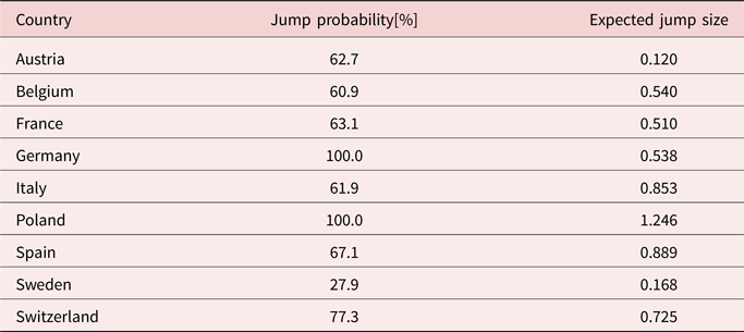
Table 3 displays the probabilities and expected sizes of a mortality jump conditional on the observed period effect change in 2020 according to the jump model (8). Apart from one exception, jump probabilities are larger than 60%. However, jump severities differ significantly by country. Furthermore, we have observed that in order to obtain sensible estimates, a sufficiently long history of mortality data is necessary. For some populations with relatively short mortality history (e.g., German males or Polish males), estimated jump probabilities are close to 100%, but the expected jump size is 0 because not enough historical mortality jump observations are available to calibrate an informative jump severity distribution.



3.4. Model parameters
We expect the additional parameters introduced by the POT, jump, and RS models to have a stabilizing effect on μ and σ, the drift and volatility of the period effect increments when mortality rates are normal. The lacking robustness of the RWD drift parameter is a well-known issue even under normal mortality and has been termed recalibration risk by Cairns (Reference Cairns2013).
Figure 4 shows μ and σ of the shock models, comparing them to the RWD over two different calibration periods. When including the year 2020 in the calibration data set, μ and σ under the RWD clearly increase for all the countries. Considering the other models, these parameters are indeed less influenced by the extreme behavior of 2020 and there are only a few larger changes. For example, the volatility for Switzerland under the RS model increases. This is not surprising since the mortality shock in this country has not been large enough to lead to a regime change (see Figure 3), so that the observation of 2020 is used to calibrate μ and σ, increasing both.
Model parameters μ and σ calibrated on the years 1990–2019 or 1991–2020 of the jump, peaks-over-threshold (pot), regime switching (rs), and random walk with drift (rwd) models.

3.5. Comparing the quality of fit
As all our models are calibrated via maximum likelihood estimation, a natural way of comparing their in-sample behavior consists in comparing their likelihoods. To account for the different number of parameters we consider the Bayesian information criterion

where ${\rm L}_{\rm max}$ is the model log-likelihood, n obs the number of observations, and ${\rm n}_{\rm par}$
 the number of free parameters [see Cairns et al. (Reference Cairns, Blake, Dowd, Coughlan, Epstein, Ong and Balevich2009) for a previous application of the ${\rm BIC}$
 to compare mortality models]. This penalizes the likelihood, giving preference to more parsimonious models. The likelihood and the number of observations are calculated on the 30 years of data on which the LC parameters and the period effect drift and volatility are calibrated. For the shock models, we are actually including more information in the model by the calibration procedure described in section 2.4. We account for this by including the shock parameters θ in the total number of free parameters. This means we fully penalize for the increased model complexity, although these parameters are fixed in a first calibration step and the remaining parameters are calibrated conditional on θ. Admittedly, this is a somewhat non-standard application of the ${\rm BIC}$
 , but the results can nevertheless be assumed to give a good indication as to the balance of quality of fit and parsimony achieved by the models.
The ${\rm BIC}$ values of our models per country are displayed in Figure 5. The RWD mostly does not fit well, regardless of whether an underlying normal or lognormal distribution is assumed. In some cases, using a more general ARIMA model leads to better performance, but apart from Austria and Switzerland this is not optimal, either. The intervention model approach achieves low BIC values but is conceptually questionable due to its model structure, which does not allow for the future occurrence of non-normal mortality shocks. The shock models are more heavily penalized due to their higher number of parameters. The RS and jump models only in a few cases achieve a decrease in ${\rm BIC}$
 compared to the RWD. The POT model has low ${\rm BIC}$
 for all countries, which shows that the POT-based model adjustment improves the quality of fit even after accounting for the increased model complexity.
${\rm BIC}$ for models calibrated on data from 1991 to 2020. The black dashed line is at the level of the best-fitting model.

3.6. Backtest
In section 3.2, we have already performed a backtest to determine the calibration method for the POT, jump, and RS models, and we have found that the approach proposed in section 2.4 leads to better point forecasts. Here, using this new calibration method, we do another backtest to evaluate how the different models listed in Table 1 would have performed in the past.Footnote 7 Analogously as in section 3.2, we calibrate the models on data from 1981 to 2010 (except for the shock parameters, which are also calibrated on all available data before 1981) and evaluate them on 2011–2020. For further details on backtesting methods for stochastic mortality models, we refer to Dowd et al. (Reference Dowd, Cairns, Blake, Coughlan, Epstein and Khalaf-Allah2010), where the approach we take here is termed an expanding horizons backtest.
In Figure 6, we display the point forecast errors measured by MdAPE as defined in (15). We observe an increase over time, which is plausible as mortality rates further in the future are harder to predict and forecasting errors tend to accumulate over time, with a peak in the shock year 2020. Differences between the models are negligible.
Point and interval forecast performance measures from 2011 to 2020 (models calibrated on data from 1981 to 2010). (a) Point forecast errors, (b) interval coverage probability.

The situation is different for interval forecasts as measured by the prediction interval coverage probability

where ${1}$ denotes an indicator function and $[ \hat {m}_{x, t}^{i, {\rm lower}},\; \hat {m}_{x, t}^{i, {\rm upper}}]$
 is the 95% prediction interval implied by the model, which is calculated by Monte Carlo simulation or explicit formulae, if available [see section 2 and Schnürch et al. (Reference Schnürch, Kleinow, Korn and Wagner2022)]. It seems that the RWD as well as the more general ARIMA model and the intervention model underestimate the uncertainty in their forecasts, in particular for the shock year 2020. Assuming a lognormal instead of a normal distribution does not lead to significant changes of the PICP. The jump model has the highest PICP initially, but it then decreases over time. This is due to its model structure and will be discussed further in section 3.7. The POT model and particularly the RS approach outperform the other methods for longer forecasting horizons. However, for the RS model this comes at the cost of very wide prediction intervals in some cases so that its intervals are more reliable but less informative.
The PICP is well below 95% for all models and time points. This is due to the fact that we ignore some sources of uncertainty in our consideration. For example, the prediction intervals could be extended to include parameter uncertainty via a bootstrapping approach [Koissi et al. (Reference Koissi, Shapiro and Högnäs2006)].
As a robustness check, we have repeated the above evaluation for 99.5% prediction intervals and have found that the results are qualitatively similar.
3.7. Period effect forecasts
In this section, we illustrate the differences in period effect forecasts between the standard choice for a time series model, which is the RWD, and selected alternatives. In Figure 7, we display the observed period effects $\hat {\kappa }_t$ , t = 1991, …, 2020, and their point and 95% interval forecasts according to the RWD, jump, POT, and RS models. For Sweden, a population with rather small estimated jump probability and size (see Table 3), all point forecasts use a jump-off value equal or close to $\hat {\kappa }_{2020}$
 , and mostly agree in their trend, staying relatively similar over time. Interval forecasts differ significantly: the jump model has the most narrow intervals, followed by the standard RWD approach. The POT model has almost the same lower interval bounds as the RWD, but its upper bounds are more conservative. The RS model has the widest intervals except in the first few years. This is probably due to its two quite distinct regimes (μ = −0.23, σ = 0.14 vs. m = −0.10, s = 0.96).
Observed period effects $\hat {\kappa }_t$ , t = 1991, …, 2020, as well as point and 95% interval forecasts $\hat {\kappa }_t$
 of selected models, t = 2021, …, 2049. Intervals obtained by closed-form expressions (RWD) or Monte Carlo simulation (jump, POT, RS). (a) Sweden, (b) Poland

In contrast, point forecasts visibly differ between models for Poland, which has experienced a relatively large shock to its 2020 period effect. In particular, the jump model reverts much of this shock before forecasting so that its central projection is more optimistic than that of the other models. Still, POT and RS predict a stronger decreasing trend than RWD. Prediction interval width is largest for the RWD, which is probably due to the fact that the 2020 mortality shock leads to a large increase in period effect volatility. The other models are able to (partially) capture this volatility in their shock parameters (s in the jump and RS model, the GPD parameters in the POT model), which usually have a smaller impact on prediction intervals than volatility at “normal” times.
For an easier visual comparison of all models and countries, we display point and interval forecasts in the last forecast year, $\hat {\kappa }_{2050}$ , in Figure 8. Allowing for a more general ARIMA process (auto.arima) than the RWD tends to decrease point forecasts and leads to more narrow prediction intervals for some countries (e.g., Belgium), which is possibly due to ARIMA models generally not putting as much emphasis on the last observed value $\hat {\kappa }_{2020}$
 as the RWD. Modeling the period effect with a lognormal distribution leads to almost identical point forecasts as the RWD, whereas the prediction intervals have a tendency to be slightly narrower. Unsurprisingly, the intervention and best estimate approaches are more optimistic than the RWD, with lower point forecasts in all countries. Their prediction intervals are narrower because they ignore the extreme observation of 2020.
Country-specific period effect point and 95% interval forecasts for the year 2050, $\hat {\kappa }_{2050}$ , comparing different time series forecasting methods. Intervals obtained by closed-form expressions or Monte Carlo simulation.

The jump model usually has lower point forecasts than the RWD because jumps vanish after one period, which is implemented by reducing $\hat {\kappa }_{2020}$ by the expected jump size before using it as the forecast jump-off value, see section 2.3. The model also tends to have narrow prediction intervals. A look at the parameters indicates that it separates the period effect increment distribution into two components: a normal component with low drift μ and low volatility σ and a shock component with higher, usually positive drift m and volatility s > 0. The influence of the shock component for long-term forecasts is small compared to the influence of the normal component because the jumps are modeled as transitory, so they do not have a lasting impact. Therefore, the reduction in normal volatility σ compared to an ordinary RWD model can lead to lower prediction uncertainty.
The RWD, POT, and RS point forecasts are broadly similar and there is no country-independent tendency regarding their order. For a few countries (e.g., Italy), the RS prediction intervals are substantially wider than the RWD intervals, which is due to the high estimated volatility (e.g., s = 1.7) in the shock regime combined with the non-negligible probability of transitioning into this regime from the normal state (e.g., $p_{12} = 4.9\%$ ). It is visible that POT and RS put higher emphasis on (upward) mortality shocks because the prediction intervals are often asymmetric with a wider upper part.
3.8. Life insurance and annuity values
The mortality forecasts of our models can be summarized and we can obtain a better understanding of model risk by calculating life insurance and annuity values [see Richards and Currie (Reference Richards and Currie2009); Schnürch et al. (Reference Schnürch, Kleinow, Korn and Wagner2022)]. For this, we assume a constant yearly discount factor $v = {1\over 1.005}$ , which is a simplification allowing us to focus on the differences in mortality forecasts. As a typical example we consider a term assurance issued to a life aged x = 35 at the start of year t = 2021 which runs for n = 30 years and pays an amount of 1 at the end of the year if the life has died within this year. Its present value is given by

Here, we have used the approximation p x,t ≈ exp ( − m x,t) [Pitacco et al. (Reference Pitacco, Denuit, Haberman and Olivieri2008), Chapter 2.3].
Similarly, we determine the present value of a temporary annuity-immediate for a life aged x = 65 at the start of year t = 2021 running for n = 30 years, denoted by $a_{x\, \colon \, {\overline{n}\vert}}( t)$ . We calculate intervals for annuity and life insurance values by inserting the 95% prediction interval bounds for the death rates into the annuity and life insurance valuation formulae.Footnote 8
Figure 9 shows life insurance values implied by the different models. Annuity values are shown in Figure 12 (Appendix B). Observations from these figures are mostly analogous to the ones about period effect forecasts in section 3.7.
Country-specific life insurance values $A_{35\, \colon \, {\overline{30}\vert}}( 2021)$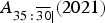 based on point and interval death rate forecasts, comparing different time series forecasting methods. Discount factor $v = {1\over 1.005}$
 . The bars are obtained by inserting the 95% prediction interval bounds for the death rates into (18).

3.9. Model performance under different future scenarios
It would be useful to get some impression of the future forecasting accuracy of the different models. This is complicated by the fact that the occurrence of mortality shocks and the further course of the COVID-19 pandemic are very hard to predict. While most scientists believe that a transition to an endemic phase is the most likely trajectory and a worldwide elimination of the virus is considered almost impossible [Scudellari (Reference Scudellari2020); Phillips (Reference Phillips2021)], it is unclear how long such a transition will take and how severe the disease will continue to be.
Telenti et al. (Reference Telenti, Arvin, Corey, Corti, Diamond, García-Sastre, Garry, Holmes, Pang and Virgin2021) describe three future scenarios: (i) ongoing high levels of infection and severe disease due to the inability to gain rapid control over COVID-19, (ii) transition to an endemic seasonal disease similar to influenza, which has a yearly global death toll approximately between 250000 and 500000, (iii) transition to an endemic disease similar to other existing human coronavirus infections with significantly lower impact on population health and mortality. This last state could, however, take decades to reach or may not occur at all. They further note that the probability of occurrence is hard to quantify for any of these scenarios due to material gaps in current scientific knowledge.
Another aspect influencing the assessment of future mortality development is the possibility that SARS-CoV-2 might reoccur years after the alleged end of the COVID-19 pandemic, for instance by spilling back from animal reservoirs into the human population [Phillips (Reference Phillips2021)]. Brüssow (Reference Brüssow2021) points out that COVID-19 displays clinical similarities to the 1889 Russian flu pandemic, which lasted for several years and then possibly reappeared around ten years later. As a related alternative, a new mortality shock might arise, for example, in the form of another pandemic caused by a different pathogen such as MERS-CoV: “the risk for MERS-CoV evolving into a more transmissible virus should not be underestimated” [Telenti et al. (Reference Telenti, Arvin, Corey, Corti, Diamond, García-Sastre, Garry, Holmes, Pang and Virgin2021)]. It is impossible to predict the exact time, but it is highly likely that further pandemics will emerge: “the question is not if, but when” [World Health Organization (2021)].
With these considerations in mind, we define five exemplary 30-year scenarios of future mortality with a focus on the development of COVID-19 and the occurrence of new mortality shocks. Detailed definitions of these scenarios are provided in Appendix A. Generally, two of them are relatively optimistic (second wave in 2021 and normality afterwards; only short-term mortality impairments), while the others are more pessimistic (occurrence of another pandemic in 2034; occurrence of another pandemic in 2048; persistent consequences of the COVID-19 pandemic). Our scenarios for the future impact of COVID-19 on mortality are inspired by the ones considered by Continuous Mortality Investigation (2020). For the scenarios including the occurrence of a further pandemic, we have chosen the years 2034 and 2048 arbitrarily for illustrative purposes. Zhou and Li (Reference Zhou and Li2021) show how to include expert opinions about disease transmission and infection fatality rates on the short term and about the reoccurrence of a COVID-alike pandemic on the longer term in the definition of mortality scenarios.
In order to get a better impression of each model's forecasting behavior, we evaluate its average and worst-case performance over our five scenarios. Figure 10 shows the results of this evaluation.
Point and interval forecast errors over different future mortality scenarios, average and worst case. Model calibrated on data from 1991 to 2020.

The models usually achieve their worst performance in the most pessimistic scenario, which assumes a persisting interruption of mortality improvements. The best estimate and intervention models are the least robust with respect to this scenario and have the highest worst-case MdAPE and lowest worst-case PICP. The remaining models have similar point forecasts and, therefore, similar average and worst-case performances (the jump model is a slight exception). However, the prediction intervals of the POT and the RS model are more robust with respect to their worst-case errors compared to the RWD.
With a scenario-based approach, model choice can be grounded upon the beliefs of the modeler by assigning subjective probabilities to each of the scenarios, calculating a correspondingly weighted average of the error measures under each scenario and choosing the model which minimizes this weighted average. Of course, this requires sufficient information to estimate occurrence probabilities, which will only be obtained over time.
4. Conclusion
Depending on the considered population, the usual RWD is not always appropriate for modeling the LC period effects because it relies on a normal distribution assumption, which is not robust toward mortality shocks. In particular, the excess mortality induced by COVID-19 strongly influences point forecasts in the short term and interval forecasts even in the long term [Schnürch et al. (Reference Schnürch, Kleinow, Korn and Wagner2022)].
In this work, we have demonstrated that simply switching to a different distribution such as the lognormal without structurally modeling mortality shocks does not sufficiently address this issue. General outlier adjustment methods such as an intervention model improve the fit and allow to keep the normal distribution assumption, but they have poorer backtest performance as regards prediction uncertainty quantification (section 3.6), and both their point and interval forecasts would be significantly inferior in an adverse mortality scenario (section 3.9).
We therefore recommend to not exclude the death rates of 2020 from the training data of the LC model nor to use an intervention model, unless mortality shocks are not deemed relevant for the application. Otherwise, the mixture model approach based on the POT method looks most appropriate in our empirical investigations. It yields a better fit as well as more stable and reliable interval forecasts than the RWD. Depending on the views of the modeler on future mortality trends, an additional adjustment to diminish the persistence of the 2020 shock in its forecasts may be advisable (see the remark at the end of section 2.3).
While being conceptually intriguing, the RS approach has rather high ${\rm BIC}$ values and yields very wide prediction intervals. The jump model leads to more narrow prediction intervals, which indicates that it in fact works as intended (see the explanation in section 3.7). It further contains an explicit adjustment of the forecast jump-off value to remove the impact of a shock, which is based on estimations of shock probability and size given the observed period effect change. However, its PICP decreases over time in the backtest and its quality of fit is suboptimal for most populations.
In any case, if using one of the three shock models, we have demonstrated in section 3.2 that it is clearly beneficial to calibrate the time series parameters relating to the shock events on a larger data set than the LC and the normal time series parameters (μ, σ) instead of calibrating all the parameters on the same large data set as proposed in the literature so far.
There are several directions for extensions and further research:
• In some countries, the COVID-19 pandemic might have affected old-age mortality more than young-age mortality. This is not reflected in the model approaches we have considered, as they only account for shocks which follow the same age pattern as general mortality improvements. One could address this by introducing shock-specific age effect parameters [Liu and Li (Reference Liu and Li2015)]. However, this complicates calibration, among other reasons due to sparsity of data on mortality shock events. An alternative is to incorporate expert opinions, which could not only relate to age patterns of COVID-19 mortality but also to its future development and the occurrence of new pandemics [Zhou and Li (Reference Zhou and Li2021)]. This delicate issue is beyond the scope of this paper, and it certainly deserves further investigation.
• At the moment of writing, COVID-19 is expected to significantly affect mortality in 2021 as well, thus inducing a longer-lasting mortality shock. Such an effect is explicitly modeled only by the RS model, where it corresponds to a longer-lasting stay in the shock regime. It could be incorporated in the jump model as well by modeling a serial correlation in the Bernoulli process governing the occurrence of jumps or even in the jump severities. Again, this would not be easy to calibrate. A simpler alternative is to reformat the data in two-year instead of one-year time intervals. This trivially allows to explicitly model shocks of up to two years. However, modeling in two-year intervals is somewhat unusual and reduces the available data by half.
• Instead of ordinary prediction intervals, we could consider highest-density regions as proposed by Hyndman (Reference Hyndman1995) to better account for multimodality of the jump and RS models. These regions can consist of several intervals, one for each mode, and therefore yield a more informative distributional prediction for future mortality rates.
• We have focused on the LC model, but the presented approaches are in principle applicable for other stochastic mortality models as well. It would be particularly interesting to consider models with more than one factor, which could require some multi-dimensional generalizations of the approaches from section 2.3.
• We have modeled all populations in isolation. One could instead consider a multi-population approach where all countries or groups of similar countries share the same shock parameters. Analogous ideas have been investigated in the literature for other parameters of stochastic mortality models [Li and Lee (Reference Li and Lee2005); Kleinow (Reference Kleinow2015); Schnürch et al. (Reference Schnürch, Kleinow and Korn2021)], and a first proposal in this direction has been made by Zhou et al. (Reference Zhou, Li and Tan2013). However, in contrast to “normal” mortality, it is not implausible that the effects of mortality shocks can be strongly country-specific (e.g., German mortality in 2020 has been less affected by COVID-19 than in several neighboring countries). In fact, we have compared the parameters obtained over the considered populations, and they are usually quite different. Given that for some of the parameters, such as the RS probability p 12, even small differences can lead to large effects, we have refrained from implementing such an approach.
Acknowledgements
We would like to express our gratitude to the anonymous referee for the constructive comments. Furthermore, we thank Ralf Korn and Stephen Richards for helpful discussions. S. Schnürch is grateful for the financial support from the Fraunhofer Institute for Industrial Mathematics ITWM. T. Kleinow acknowledges financial support from the Actuarial Research Centre of the Institute and Faculty of Actuaries through the research program on “Modelling, Measurement and Management of Longevity and Morbidity Risk.”
Appendix A: Defining scenarios of future mortality
We define a 30-year mortality scenario by specifying improvement rates

for $x\in {\cal X}$ and t = 2021, …, 2050. We consider five scenarios:
∙ Second wave in 2021 and normality afterwards:
(A2)$${I_{x, 2021} = 0,\; I_{x, 2022} = 1 - {1\over 1-I_{x, 2020}},\; I_{x, t} = I_{x, t-31}\;{\rm for }\; t = 2023,\; \ldots,\; 2050. }$$In particular, we have m x,2022 = m x,2019 and “normality” means that we observe exactly the same sequence of improvement rates between 2023 and 2050 as between 1982 and 2019.∙ Short-term impairments:
(A3)$$\eqalign{I_{x, 2021} &= {I_{x, 1990} - I_{x, 2020} - 0.04\over 1 - I_{x, 2020}},\; I_{x, 2021 + h} = I_{x, 1990 + h} - 0.01( 4-h) \;{\rm for }\; h = 1,\; 2,\; 3,\; I_{x, t} = I_{x, t-31}\; \cr {\rm for }\; t &= 2025,\; \ldots,\; 2050. }$$In particular, we have m x,2021 = (1.04 − I x,1990)m x,2019.∙ Second wave in 2021 and normality afterwards until another pandemic inducing a larger shock than COVID-19 (with identical age structure) emerges in 2034:
(A4)$$\eqalign{I_{x, 2021} &= 0,\; I_{x, 2022} = 1 - {1\over 1-I_{x, 2020}},\; I_{x, t} = I_{x, t-31}\;{\rm for }\; t = 2023,\; \ldots,\; 2033,\; I_{x, 2034} = \left(2I_{x, 2020}\right)^-,\; \cr I_{x, 2035} &= 0,\; I_{x, 2036} = 1 - {1\over 1-I_{x, 2034}},\; I_{x, t} = I_{x, t-31}\;{\rm for }\; t = 2037,\; \ldots,\; 2050. }$$In particular, we have m x,2022 = m x,2019 and m x,2036 = m x,2033.∙ Second wave in 2021 and normality afterwards until another pandemic inducing a larger shock than COVID-19 (with identical age structure) emerges in 2048:
(A5)$$\eqalign{I_{x, 2021} &= 0,\; I_{x, 2022} = 1 - {1\over 1-I_{x, 2020}},\; I_{x, t} = I_{x, t-31}\;{\rm for }\; t = 2023,\; \ldots,\; 2047. I_{x, 2048} = \left(2I_{x, 2020}\right)^-,\; \cr I_{x, 2049} &= 0,\; I_{x, 2050} = 1 - {1\over 1-I_{x, 2048}}. }$$In particular, we have m x,2022 = m x,2019 and m x,2050 = m x,2047.∙ Persistent reduction in improvement rates, leading to zero average improvement between 2022 and 2050,
(A6)$${I_{x, 2021} = {I_{x, 1990} - I_{x, 2020} - g\over 1 - I_{x, 2020}},\; I_{x, t} = I_{x, t-31} - g \;{\rm for }\; t = 2022,\; \ldots,\; 2050,\; }$$where $g\, \colon = {1\over 29} \sum _{t = 1991}^{2019} I_{x, t}.$ In particular, we have m x,2021 = (1 + g − I x,1990)m x,2019.


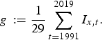
Note that we do not make a statement about the probabilities of any of these scenarios becoming reality. The development of mortality rates under the five scenarios is shown in Figure 11 for chosen countries and age groups.
Development of mortality rates for the German, Polish, and Spanish populations in the age groups 50–54, 70–74, and 90+ between 2021 and 2050 under the five scenarios defined above.

Appendix B: Annuity values
Country-specific annuity values $a_{65\, \colon \, {\overline{30}\vert}}( 2021)$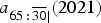 based on point and interval death rate forecasts, comparing different time series forecasting methods. Discount factor $v = {1\over 1.005}$
 . The bars are obtained by calculating annuity values based on the 95% prediction interval bounds for the death rates.