1 Introduction
A laminar boundary layer developing along an aerodynamic surface may separate if exposed to a sufficiently strong adverse pressure gradient. Under certain conditions, the increase of momentum exchange due to laminar to turbulent transition in the separated shear layer may lead to reattachment. Therefore, in the time-average sense, a closed recirculation region forms near the surface, namely a laminar separation bubble (LSB, Gaster Reference Gaster1967).
Due to the requirement of a laminar boundary layer state at the separation location, this phenomenon is usually observed at low to moderate Reynolds numbers, typical in applications such as glider or unmanned aerial vehicle wings and turbomachine blades. The transition process associated with LSBs is highly susceptible to environmental disturbances and the resulting separated shear layers are inherently unstable. As a result, changes in background disturbances can lead to unwanted impact on aerodynamic performance such as stalling, loss of lift, increase of drag and noise emission. Due to these implications, numerous studies have been performed to investigate and predict LSB dynamic properties and stability characteristics (e.g. Gaster & Grant Reference Gaster and Grant1975; Dovgal, Kozlov & Michalke Reference Dovgal, Kozlov and Michalke1994; Watmuff Reference Watmuff1999). Although applications primarily involve aerofoils, LSBs driven by an adverse pressure gradient on a semi-infinite flat plates exhibit the relevant fundamental effects and have been used as a suitable experimentation and computation platform (e.g. Gaster Reference Gaster1967; Marxen & Rist Reference Marxen and Rist2010).
Whether numerical or experimental, most studies that investigate stability characteristics involve artificial forcing of the boundary layer with known perturbations at a location upstream of the LSB separation point and describe the subsequent flow evolution. The most common type of forcing is sinusoidal and periodic at the most unstable frequency of the separated shear layer, usually identified through linear stability theory (LST) analysis. This type of forcing has been introduced by various means including spanwise-uniform wall oscillation (Alam & Sandham Reference Alam and Sandham2000; Marxen et al. Reference Marxen, Lang, Rist, Levin and Henningson2009), externally imposed acoustic excitation (Yarusevych, Sullivan & Kawall Reference Yarusevych, Sullivan and Kawall2007; Jones, Sandberg & Sandham Reference Jones, Sandberg and Sandham2010) as well as dielectric barrier discharge (DBD) plasma actuation (Yarusevych & Kotsonis Reference Yarusevych and Kotsonis2017). However, the majority of the previous studies considered the response of the LSB to continuous forcing. Gaster & Grant (Reference Gaster and Grant1975) were the first to introduce an impulsive disturbance, exciting the full spectrum of instability modes, thus generating a wave packet through selective amplification. This method was subsequently used by Watmuff (Reference Watmuff1999) and Diwan & Ramesh (Reference Diwan and Ramesh2009). It must be noted that impulsive disturbances have, so far, been locally introduced at a single point, usually a pressure tap. Consequently, the emerging wave packets initially exhibit strong three-dimensional features, which complicates the elucidation of the underlying physical mechanisms and application of LST. The present study, instead, focuses on two-dimensional spanwise-uniform impulsive disturbances.
In the laminar part of the LSB, flow is essentially considered two-dimensional and parallel. If, in addition, small perturbations to the baseline flow are assumed, it is possible to apply linear stability theory for estimating the most amplified unstable mode frequency. Häggmark, Hildings & Henningson (Reference Häggmark, Hildings and Henningson2001), Rist & Maucher (Reference Rist and Maucher2002) and Marxen & Rist (Reference Marxen and Rist2010) demonstrated that LST applied to the mean baseline flow can successfully reproduce experimental and numerical stability observations. It is generally accepted that disturbances developing in a LSB are initially convectively amplified via a Kelvin–Helmholtz instability mechanism, similar to free shear layers (Ho & Huerre Reference Ho and Huerre1984; Watmuff Reference Watmuff1999; Marxen et al. Reference Marxen, Kotapati, Mital and Zaki2015). Inviscid inflectional and Göertler type instability mechanisms have been proposed by Diwan & Ramesh (Reference Diwan and Ramesh2009) and Marxen et al. (Reference Marxen, Lang, Rist, Levin and Henningson2009) respectively. Furthermore, Theofilis, Hein & Dallmann (Reference Theofilis, Hein and Dallmann2000) conjectured a self-exciting, globally unstable process in a disturbance-free numerical environment. In practice, convective amplification of disturbances in the separated shear layer leads to the formation of initially two-dimensional vortical structures which manifest as coherent vortex shedding (Jones, Sandbergh & Sandham Reference Jones, Sandbergh and Sandham2008; Hain, Kähler & Radespiel Reference Hain, Kähler and Radespiel2009; Serna & Lázaro Reference Serna and Lázaro2014; Kurelek, Lambert & Yarusevych Reference Kurelek, Lambert and Yarusevych2016). Once they reach the aft part of the LSB, these spanwise structures undergo three-dimensional breakdown, the underlying mechanism of which is the subject of active investigations. Marxen, Lang & Rist (Reference Marxen, Lang and Rist2013) summarise three instability mechanisms that can take place in LSBs: ‘primary global’, ‘secondary’ and ‘highly localised’ instabilities. Primary global instabilities refer to the entire bubble and are typically of low frequency. For a fully global instability to develop, Theofilis (Reference Theofilis2011) reports a requirement of reverse flow of the order of 10 % of the free stream velocity. On the other hand, Alam & Sandham (Reference Alam and Sandham2000) report that reverse flow between 15 % and 20 % is required for a local absolute instability. Secondary instabilities are absolute and involve vortex shedding. They are either elliptic, causing three-dimensional deformation of vortex cores, or hyperbolic, affecting the braid region between two consecutive vortices. Finally, highly localised instabilities are of small scale and manifest in high-shear layers. They have been shown to play a role in hairpin vortex formation (Bake, Meyer & Rist Reference Bake, Meyer and Rist2002).
Rist & Augustin (Reference Rist and Augustin2006) and Marxen & Rist (Reference Marxen and Rist2010) documented enhanced flow stabilisation with increasing forcing amplitude. Additionally, they observed reduction of the LSB size from both upstream and downstream directions. Similarly to Dovgal et al. (Reference Dovgal, Kozlov and Michalke1994) and Boiko et al. (Reference Boiko, Grek, Dovgal and Kozlov2002), they suggested a feedback loop process to explain the bubble size reduction due to controlled disturbances. More specifically, a disturbance input alters the flow in the aft part of the bubble, resulting in a global change of pressure gradient due to viscous–inviscid interactions. This indirectly distorts the mean flow at the upstream part of the bubble towards a more stable state, mitigating subsequent disturbance amplification, effectively leading to stabilisation. Marxen & Henningson (Reference Marxen and Henningson2011) argued that, if irregular disturbances are present in the incoming flow, such as free stream turbulence in free flight or wind tunnel experiments, the aforementioned feedback loop may explain the occurrence of an intermittent shear layer fluctuation associated with LSBs, often referred to as ‘flapping’ (e.g. Zaman, McKinzie & Rumsey Reference Zaman, McKinzie and Rumsey1989). Adding to this argumentation, significant reduction of the flapping behaviour due to artificial monochromatic forcing has been noted by Dovgal & Boiko (Reference Dovgal, Boiko, Fasel and Saric1994) and Sandham (Reference Sandham2008), related to the locking of the bubble dynamics to modes of constant amplitude. Moreover, flow stabilisation due to the mean flow deformation under continuous forcing has recently been confirmed experimentally by Yarusevych & Kotsonis (Reference Yarusevych and Kotsonis2017).
Laminar separation bubbles are often classified in literature as ‘short’ or ‘long’ based on their length or whether their influence on pressure distribution is global or local (Owen & Klanfer Reference Owen and Klanfer1955; Tani Reference Tani1964; Gaster Reference Gaster1967). A detailed overview of the associated bubble characteristics is given by Marxen & Henningson (Reference Marxen and Henningson2011). Pauley, Moin & Reynolds (Reference Pauley, Moin and Reynolds1990) noted that long separation bubbles with laminar reattachment do not exhibit formation of vortex shedding. In contrast, the long separation bubbles of Gaster (Reference Gaster1967) and Marxen & Henningson (Reference Marxen and Henningson2011) exhibit laminar to turbulent transition and turbulent reattachment. However, they fail to reattach as early as short bubbles. Marxen & Henningson (Reference Marxen and Henningson2011) note that, contrary to short separation bubbles, vortex roll up in long bubbles occurs further downstream of the transition location. Under certain conditions, involving minor flow variations, a short separation bubble may significantly elongate, a dynamic process termed ‘bursting’ which has been associated with aerofoil stall by Sandham (Reference Sandham2008). It should be noted, however, that bursting and elongation do not necessarily imply that the LSB acquires long bubble characteristics. Although determining appropriate criteria for bubble bursting has been a recurrent topic (Gaster Reference Gaster1967; Diwan & Ramesh Reference Diwan and Ramesh2009; Marxen & Henningson Reference Marxen and Henningson2011; Serna & Lázaro Reference Serna and Lázaro2015), the development of a universal criterion has proven difficult, mainly due to the lack of sufficient understanding of the bursting process.
In an effort to characterise short and long bubbles, Gaster (Reference Gaster1967) initiated bursting by reducing the wind tunnel speed, affecting pressure gradient and free stream turbulence. Following a different approach, Marxen & Henningson (Reference Marxen and Henningson2011) induced bursting by eliminating or attenuating disturbances in their direct numerical simulation (DNS) boundary conditions. Both studies, therefore, relied on artificial reduction of the amplitude of disturbances in the separated shear layer. It must be noted here, that although this approach is technically straightforward in experimental and numerical frameworks, it does not correspond fully to the physical sequence of events preceding bubble bursting. The reason is the inability of these approaches to decouple the effect of local mean flow stability changes (i.e. mean flow deformation) and the effect of incoming perturbation amplitude, since the latter is varied. Nevertheless, based on these studies, a hypothesis can be formulated regarding global changes of the size of LSBs as a function of incoming disturbances which could lay the foundation for elucidating both the flapping and bursting mechanisms (Marxen & Henningson Reference Marxen and Henningson2011). Namely, the amplitude of flow perturbations entering the LSB defines the breakdown location which, in turn, defines the size of the LSB and the growth of the developing instabilities. The evaluation of such a hypothesis in an experimental framework is the premise of the present study, in reference to the numerical study of Marxen & Henningson (Reference Marxen and Henningson2011).
This work investigates the response of laminar separation bubbles to impulsive forcing by assessing the attendant changes of flow dynamics and the underlying stability mechanism. Through the above, further insight is provided into both flapping and bursting mechanisms. A laminar separation bubble is induced on a flat plate by an externally imposed adverse pressure gradient. Based on the maximum reverse flow criterion, the formed LSB is globally stable but convectively unstable (Gaster Reference Gaster1992; Alam & Sandham Reference Alam and Sandham2000). Repetitive, two-dimensional, impulsive disturbances are introduced upstream of the location of LSB separation point by means of a DBD plasma actuator (Corke, Enloe & Wilkinson Reference Corke, Enloe and Wilkinson2010; Kotsonis Reference Kotsonis2015; Yarusevych & Kotsonis Reference Yarusevych and Kotsonis2017). The premise of using impulsive, spanwise-uniform disturbances is twofold. Firstly, impulsive excitation features a broad spectral content, giving rise to the naturally pertinent instability modes through selective amplification. Secondly, for constant conditions (free stream velocity and turbulence levels) the inflow of the LSB experiences an elevated incoming disturbance amplitude only during the short duration of the impulse. At all other instants, the LSB experiences a natural level of incoming disturbances. Effectively, this enables monitoring mean flow deformation effects, following the wave packet convection, without altering the amplitude of incoming disturbances.
The evolution of the emerging wave packet and the response of the LSB are captured with time-resolved particle image velocimetry (PIV), demonstrating that bursting occurs shortly after the convection of the wave packet. Finally, linear stability theory is employed in order to relate pertinent changes in stability characteristics to the changes in LSB dynamics. Since the aforementioned studies (Häggmark et al. Reference Häggmark, Hildings and Henningson2001; Rist & Maucher Reference Rist and Maucher2002; Marxen & Rist Reference Marxen and Rist2010) involving linear stability theory analysis only consider stability characteristics of the mean flow, a necessity rises of investigating dynamic stability, for which quasi-steady assumptions may be made. LST in the spatial formulation is, therefore, applied on phase-averaged velocity fields within a forcing cycle in order to assess changes in stability characteristics from bursting until recovery of the LSB to its unperturbed state.
2 Experimental apparatus and techniques
2.1 Model set-up
Experiments are carried out in an open-loop wind tunnel with a square cross-section of
 $500~\text{mm}\times 500~\text{mm}$
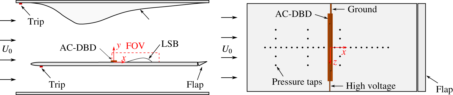
. An overview of the experimental set-up is shown in figure 1. A 20 mm thick, 500 mm wide and 1000 mm long Plexiglas® flat plate is inserted in the test section off centre at a 30 % distance from the floor for alleviating wind tunnel corner effects (Saric & White Reference Saric and White1998). The flat plate leading edge is a modified super ellipse (Lin, Reed & Saric Reference Lin, Reed and Saric1992), enabling seamless curvature change and ensuring development of laminar boundary layer. A movable flap is positioned at the trailing edge of the flat plate and is deflected such as to localise the leading edge stagnation point on the upper side of the flat plate, eliminating possible unsteady separation effects. The pressure gradient on the flat plate surface is conditioned with the aid of a flexible, 1 mm thick polycarbonate wall, positioned on the opposite side of the test section. A Cartesian coordinate system is defined such that
 $\tilde{x}=0$
lies 420 mm from the leading edge of the flat plate,
 ${\tilde{y}}=0$
at its top surface and
 $\tilde{z}=0$
at its midspan.
Schematic of the experimental set-up.

The boundary layer on the lower side of the flat plate is tripped at a distance of 50 mm from the leading edge by means of a 2 mm thick zig–zag turbulator. This is done for eliminating possible fluctuations of a laminar boundary layer as well as for reducing the strength of shedding at the trailing edge flap. The same tripping technique is applied at the upstream end of the flexible wall in order to avoid unsteady separation in the adverse pressure gradient region. Suppression of these effects was confirmed during preliminary studies by employing both tuft flow visualisation and PIV measurements. In addition, flow field surveys with a stethoscope confirmed that the boundary layer does not relaminarise in the favourable pressure gradient region.
The free stream velocity
 $(\tilde{U} _{0})$
is set using a Pitot-static tube located 100 mm upstream of the flat plate leading edge and is kept constant at
 $6.4~\text{m}~\text{s}^{-1}$
, with uncertainty lower than 2 %. Hot-wire measurements, bandpass filtered between 0.1 Hz and 1 kHz, were used to estimate free stream turbulence intensity
 $(\text{TI}=\tilde{U} _{rms}^{\prime }/\tilde{U} _{0})$
, determined to be under 0.2 %.
The pressure distribution imposed by the flexible wall is measured by means of 36 pressure taps integrated in the flat plate (figure 1) and is expressed in terms of surface pressure coefficient
 $(C_{p})$
. In the streamwise direction, pressure taps are located at the midspan (
 $\tilde{z}=0$
) with 30 mm spacing. Spanwise taps are spaced symmetrically with respect to the midspan at three streamwise locations;
 $\tilde{x}=-260$
mm,
 $-80$
mm and 100 mm, with a spanwise spacing of 50 mm. Measurements are performed with a high accuracy multi-channel pressure scanner at an acquisition frequency of 10 Hz and mean pressures are estimated from 150 samples at each location. The obtained mean
 $C_{p}$
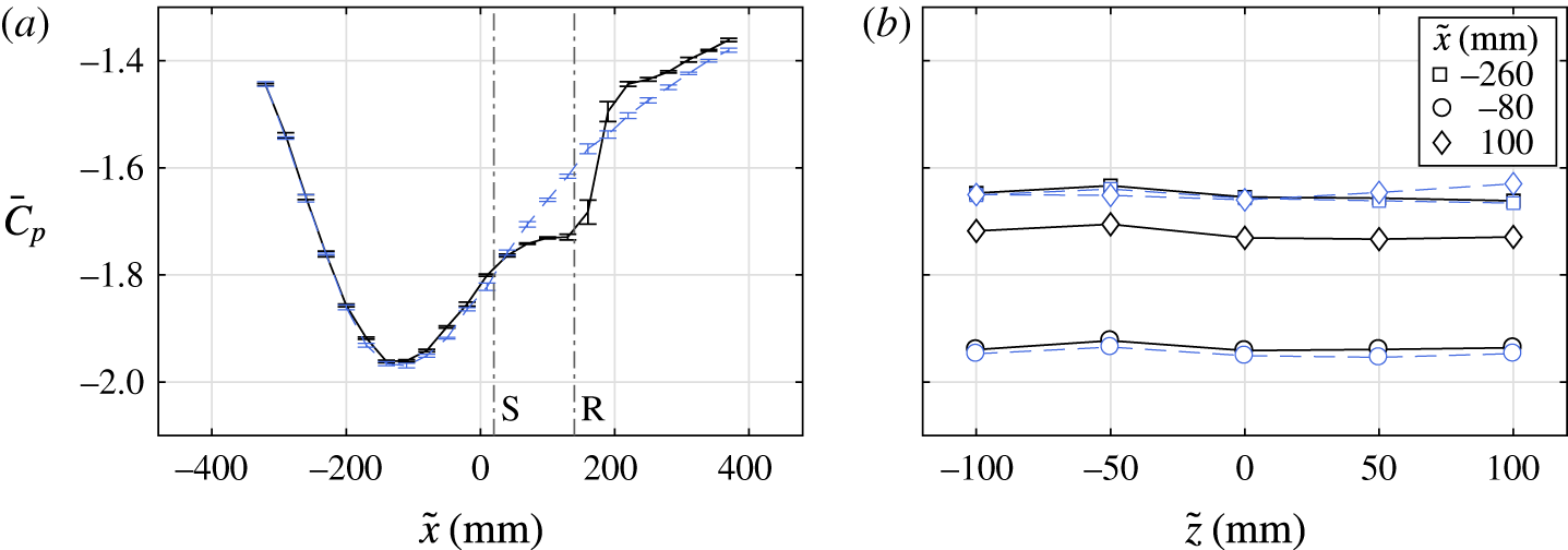
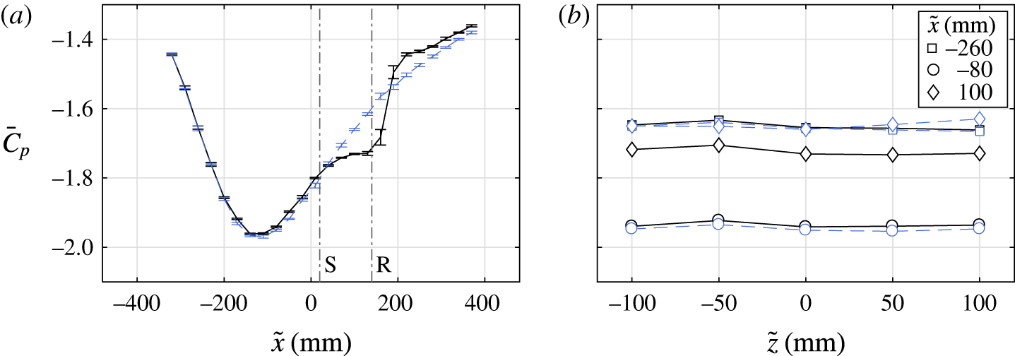
distribution is shown in figure 2. The presence of a pressure plateau in the streamwise surface pressure distribution (figure 2
a) indicates the formation of a laminar separation bubble (e.g. Yarusevych, Sullivan & Kawall Reference Yarusevych, Sullivan and Kawall2009) in the interval between
 $\tilde{x}\approx 30$
mm and
 $\tilde{x}\approx 150$
mm. The presence of a laminar separation bubble is confirmed by tripping the boundary layer with a zig–zag turbulator placed at the leading edge of the flat plate. The resulting streamwise pressure distribution (figure 2
a) shows that the turbulent boundary layer overcomes the adverse pressure gradient without separating and that
 $C_{p}$
increases downstream without exhibiting the typical for laminar separation bubbles pressure plateau. Figure 2(b) demonstrates that both clean and tripped configurations produce uniform pressure distribution in the spanwise direction, ensuring essentially two-dimensional conditions in the time-averaged sense.
 $C_{p}$
distribution in (a) streamwise direction (
 $\tilde{z}=0$
) and (b) spanwise direction. Solid lines: clean flat plate conditions; dashed lines: tripped boundary layer near the leading edge. Separation and reattachment points are noted with S and R, respectively.
2.2 AC-DBD forcing
Controlled disturbances are introduced upstream of the LSB with the use of an alternating current dielectric barrier discharge (AC-DBD) plasma actuator (Corke et al.
Reference Corke, Enloe and Wilkinson2010; Benard & Moreau Reference Benard and Moreau2014; Kotsonis Reference Kotsonis2015; Yarusevych & Kotsonis Reference Yarusevych and Kotsonis2017), located just upstream of the mean separation point (figure 1). It consists of two asymmetrically positioned electrodes, separated by a dielectric layer. When activated, the DBD plasma actuator enables momentum exchange through ion-neutral collisions resulting in the formation of a wall-parallel jet near the surface (Kotsonis Reference Kotsonis2015). Deterministic perturbations in terms of amplitude and frequency can, therefore, be introduced by manipulating the carrier signal. Being an electric device, the DBD plasma actuator has a fast response and precisely controlled frequency and amplitude. For this study, the streamwise extent of the high voltage and ground electrodes are 2 mm and 5 mm respectively. Both electrodes are painted on the surfaces using conductive silver coating and are less than 10
 $\unicode[STIX]{x03BC}\text{m}$
in thickness. The dielectric comprises of 60
 $\unicode[STIX]{x03BC}\text{m}$
thick Kapton® polyimide film, however, its thickness is significantly lower than the local boundary layer displacement thickness (
 ${\approx}5.5~\text{mm}$
). Preliminary studies have confirmed negligible influence on the bubble dynamics from the mechanical roughness associated with the actuator. The discharge gap is located at a distance of 420 mm from the leading edge and serves as the origin of the reference system (figure 1).
The actuator is driven by a digitally controlled high voltage amplifier. The forcing signal is comprised by repetitive pulses as shown in figure 3. Each pulse is constructed by modulating the sinusoidal carrier signal (
 $\tilde{f}_{c}=5$
kHz) with a square signal at significantly lower pulse frequency of
 $\tilde{f}_{p}=2$
Hz. The duty cycle of modulation is fixed at 0.2 %, resulting in a pulse width of 1 ms. As will be shown in a later section, the relevant hydrodynamic frequency associated with the primary shear layer instability in the current LSB is 136 Hz. Respectively, the frequency associated with flapping is of the order of 10 Hz. With the carrier frequency exceeding any relevant hydrodynamic frequency by at least two orders of magnitude, each 1 ms burst is essentially equivalent to a single impulsive perturbation. Furthermore, the frequency of the pulses
 $(\tilde{f}_{p}=2~\text{Hz})$
is selected such that the bubble fully recovers to its unperturbed state between two consecutive pulses. Thus, the perturbations introduced represent a sequence of statistically independent impulses, facilitating phase averaging of the flow measurements.
Sample of the DBD plasma actuator forcing signal of amplitude
 $A$
. The sinusoidal signal at carrier frequency
 $\tilde{f}_{c}=5$
kHz is modulated with a square wave of pulse frequency
 $\tilde{f}_{p}=2$
Hz. Duty cycle is 0.2 % leading to 1 ms pulse width.

In order to assess the effect of the excitation amplitude on LSB topology and dynamics, several peak to peak voltage amplitudes are considered, between 2.5 and 5 kV. Characterisation of the forcing exerted on the fluid by the AC-DBD for the applied voltages is expressed in terms of momentum coefficient
 $(\boldsymbol{C}_{\unicode[STIX]{x1D707}})$
, as formulated by Amitay et al. (Reference Amitay, Smith, Kibens, Parekh and Glezer2001).
 $$\begin{eqnarray}\boldsymbol{C}_{\unicode[STIX]{x1D707}}=\frac{\overline{\tilde{\boldsymbol{I}}}}{{\textstyle \frac{1}{2}}\tilde{\unicode[STIX]{x1D70C}}_{0}{\tilde{U} _{0}}^{2}\tilde{l}}.\end{eqnarray}$$
Here, the time-averaged momentum per unit length,
 $\overline{\tilde{\boldsymbol{I}}}$
, is normalised by the free stream fluid density,
 $\tilde{\unicode[STIX]{x1D70C}}_{0}$
, the square of the free stream velocity,
 $\tilde{U} _{0}$
and the length of the plasma actuator,
 $\tilde{l}$
. For estimating
 $\overline{\tilde{\boldsymbol{I}}}$
at each voltage, PIV measurements are carried out in quiescent conditions with the actuator operating continuously at
 $\tilde{f}_{c}=5$
kHz.
 $\overline{\tilde{\boldsymbol{I}}}$
is then calculated as described by Kotsonis et al. (Reference Kotsonis, Ghaemi, Veldhuis and Scarano2011) through application of the momentum balance equation,
 $$\begin{eqnarray}\overline{\tilde{\boldsymbol{I}}}=\oint _{s}\tilde{\unicode[STIX]{x1D70C}}_{0}\;\overline{\tilde{\boldsymbol{u}}}(\overline{\tilde{\boldsymbol{u}}}\boldsymbol{\cdot }\hat{\boldsymbol{n}})\,\text{d}\tilde{S}\end{eqnarray}$$
to the appropriate control volume,
 $S$
, assuming uniform pressure distribution. It should be noted here, that the described momentum coefficient is calculated based on continuous operation of the actuator and, as such, pertains to the mechanical power of the actuator. Since for the LSB control the actuator is operated in a modulated manner, the momentum transferred to the flow during each individual pulse can be extracted by simply multiplying the relevant momentum coefficient by the duty cycle.
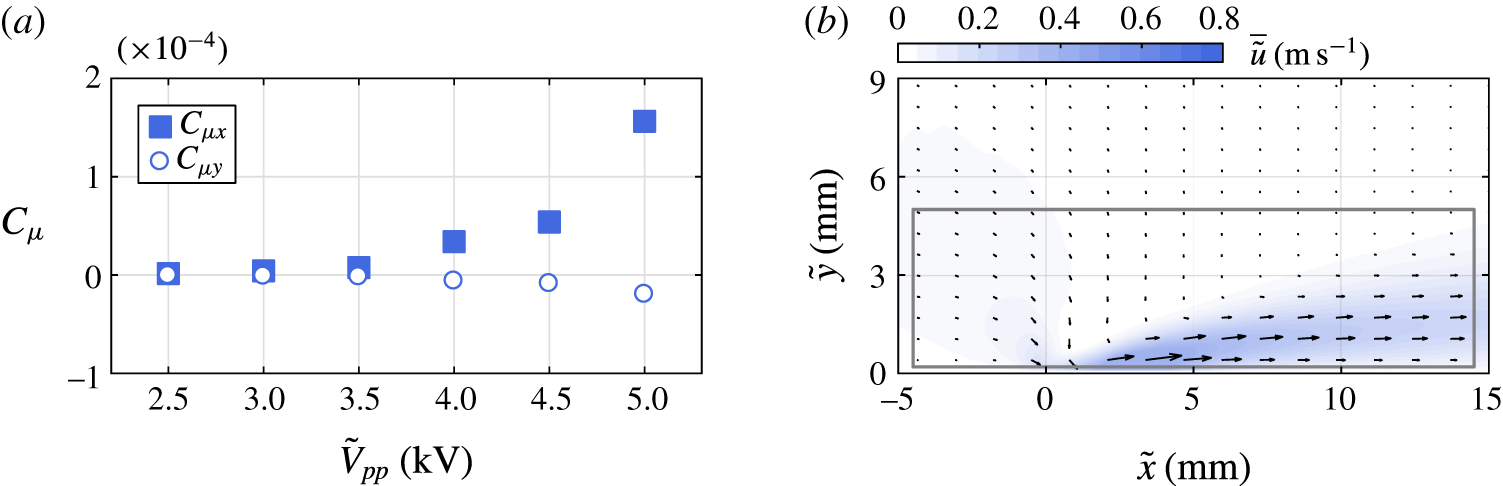
(a) DBD plasma actuator momentum coefficient as a function of applied voltage. (b) Time-averaged plasma-induced velocity field in quiescent conditions for
 $\tilde{V}_{pp}=5$
kV. The control volume boundary for the
 $\boldsymbol{C}_{\unicode[STIX]{x1D707}}$
estimation is indicated by a grey rectangle.

The estimated
 $\boldsymbol{C}_{\unicode[STIX]{x1D707}}$
during continuous operation under quiescent conditions for each applied voltage and an exemplary velocity field are shown in figure 4. Evidently, the largest contribution in forcing originates from the momentum exchange along the
 $x$
-direction
 $(C_{\unicode[STIX]{x1D707}_{x}})$
. As fluid is displaced by the jet, a secondary effect is observed in the region of the discharge gap
 $(\tilde{x}=0)$
. As a result, thrust along the
 $y$
-direction is generated towards the wall, signified by negative momentum coefficient
 $(C_{\unicode[STIX]{x1D707}_{y}})$
. Although the magnitude of momentum coefficient is proportional to the voltage,
 $C_{\unicode[STIX]{x1D707}_{y}}$
remains significantly lower than
 $C_{\unicode[STIX]{x1D707}_{x}}$
for all applied voltage amplitudes. For the remainder of the study,
 $C_{\unicode[STIX]{x1D707}}\approx C_{\unicode[STIX]{x1D707}_{x}}$
will be used as an indicator of actuator strength. Finally, it is important to note that the topology of the jet as well as the value of
 $C_{\unicode[STIX]{x1D707}}$
are largely unchanged in the case of the relatively weak external flow encountered in this study (Pereira, Ragni & Kotsonis Reference Pereira, Ragni and Kotsonis2014).
2.3 Two-component PIV
A time-resolved, two-component PIV system is employed for investigating the flow field in the
 $x$
–
 $y$
plane as seen in figure 1. Illumination is performed by a laser system that delivers green light (532 nm). The beam is transformed into a 1 mm light sheet with the aid of an array of spherical and cylindrical lenses. Two high-speed cameras with
 $1024\times 1024$
pixel sensor resolution are used to image the illuminated region. Both are equipped with 200 mm macro objectives set at an aperture of
 $f/5.6$
. Particle seeding consists of vaporised water–glycol mixture droplets of 1
 $\unicode[STIX]{x03BC}\text{m}$
diameter. Acquisition frequencies
 $(\tilde{f}_{a})$
at 250, 500 and 2000 Hz are selected for obtaining statistics and resolving high frequency phenomena accordingly. For each acquisition frequency, 10 914 cropped image pairs (
 $\unicode[STIX]{x0394}\tilde{t}=60~\unicode[STIX]{x03BC}\text{s}$
) are recorded, resulting in total acquisition times of 43.7 s, 21.8 s and 5.5 s respectively. The image pairs are acquired and processed with LaVision DaVis 8.3. The magnification factor is
 $M=0.29$
, yielding a resolution of
 $14~\text{pixel}~\text{mm}^{-1}$
for each camera. Particle displacements are calculated by applying the multi-step interrogation algorithm (Scarano & Riethmuller Reference Scarano and Riethmuller2000) from an initial window of
 $48\times 48$
pixels to a final window of
 $12\times 12$
pixels with a 75 % overlap between windows. The resulting vector spacing is 0.19 mm in both
 $x$
and
 $y$
directions. The multi-step interrogation window sizes have been selected such that the final vector spacing matches the limit of spatial resolution determined via the method described by Kähler, Scharnowski & Cierpka (Reference Kähler, Scharnowski and Cierpka2012). Vector fields from the two cameras are stitched together to obtain a combined field of view of 131 mm by 14 mm.
For the experimental data presented in this work, uncertainty is quantified using the correlation statistics method (Wieneke Reference Wieneke2015). The local error for instantaneous velocity measurements is estimated to be
 $\unicode[STIX]{x1D700}_{u}\approx 1\,\%$
in the free stream and
 $\unicode[STIX]{x1D700}_{u}\approx 10\,\%$
within the LSB. Maximum uncertainty is associated with the region of shear layer breakdown and reattachment. At this location, the uncertainty in the phase-averaged velocity fields is
 $3\,\%$
,
 $5\,\%$
and
 $8\,\%$
for acquisition frequencies of 250 Hz, 500 Hz and 2000 Hz respectively. Since the majority of results discussed in the present study pertain to an acquisition frequency of
 $\tilde{f}_{a}=500~\text{Hz}$
, the corresponding uncertainty is propagated through the analysis to yield uncertainty estimates for the location of the LSB dividing streamline
 $({<}2.5\,\%)$
and LST growth rates
 $({<}3.5\,\%)$
.
Actuation and PIV measurements are digitally controlled and synchronised. The reference time
 $\tilde{t}_{0}=0$
s is set at the moment when the actuator is activated. Subsequently, the camera shutter and laser pulse signals are used for establishing the time of the first measurement to within
 $1~\unicode[STIX]{x03BC}\text{s}$
.
3 Post-processing methodology
3.1 Notation and scaling
Throughout this report, dimensional quantities are noted by a tilde and are accompanied by the respective unit (e.g.
 $\tilde{x}$
(mm)). For non-dimensional representation, measured and computed quantities are globally normalised with representative scaling parameters from the baseline unforced LSB. More specifically, all lengths are normalised with the displacement thickness at the separation point of the unforced LSB
 $(\tilde{\unicode[STIX]{x1D6FF}}_{s_{0}}^{\ast }=2.39~\text{mm})$
. Integral boundary layer parameters are estimated based on the numerical integration of the measured time-averaged velocity field. Velocities are non-dimensionalised with the local edge velocity at separation,
 $\tilde{U} _{\infty _{s}}=8.6~\text{m}~\text{s}^{-1}$
. These two scaling factors are employed for defining the Reynolds number as
 $Re_{\unicode[STIX]{x1D6FF}_{s}^{\ast }}=\tilde{U} _{\infty _{s}}\tilde{\unicode[STIX]{x1D6FF}}_{s_{0}}^{\ast }/\tilde{\unicode[STIX]{x1D708}}=1305$
. Furthermore, they are combined for frequency scaling in the form of a Strouhal number,
 $St=\tilde{f}~\tilde{\unicode[STIX]{x1D6FF}}_{s_{0}}^{\ast }/\tilde{U} _{\infty _{s}}$
. All non-dimensional quantities are denoted by their respective symbol (e.g.
 $x=\tilde{x}/\tilde{\unicode[STIX]{x1D6FF}}_{s_{0}}^{\ast }$
,
 $u=\tilde{u} /\tilde{U} _{\infty _{s}}$
). Time-averaged quantities are identified with an overbar (e.g.
 $\bar{u}$
), whereas temporal fluctuations are marked by a dash (e.g.
 $u^{\prime }$
).
An additional scaling scheme is introduced for the comparison of forced and unforced cases. Accordingly, quantities are scaled with the respective time-averaged value pertaining to the unforced LSB for each case. For example, the separation point,
 $x_{s}$
, is scaled with the mean separation point of the unforced LSB,
 $\bar{x}_{s_{0}}$
. All scaled primary (e.g. length) and derived (e.g. vorticity) quantities, are subsequently denoted by a hat (e.g.
 $\hat{x}=x/\bar{x}_{s_{0}}$
,
 $\hat{\unicode[STIX]{x1D714}}=\unicode[STIX]{x1D714}/\bar{\unicode[STIX]{x1D714}}_{s_{0}}$
).
As mentioned in § 2.2, the LSB is cyclically forced by pulses of frequency
 $\tilde{f}_{p}=2~\text{Hz}$
. Therefore, a non-dimensional phase,
 $\unicode[STIX]{x1D719}$
, is defined based on the pulse frequency and the time interval elapsed from the preceding pulse,
 $\tilde{t}$
, reading
 $$\begin{eqnarray}\unicode[STIX]{x1D719}=\tilde{t}\tilde{f}_{p}.\end{eqnarray}$$
Consequently,
 $\unicode[STIX]{x1D719}=0$
coincides with the moment of actuation, while
 $\unicode[STIX]{x1D719}=1$
occurs after a time interval of
 $\tilde{t}=1/\tilde{f}_{p}$
, at the moment prior to the next pulse initiation. Phase-averaged quantities are denoted with chevron brackets (e.g.
 $\langle u\rangle$
).
3.2 Linear stability theory
Similarly to earlier studies (Häggmark et al. Reference Häggmark, Hildings and Henningson2001; Rist & Maucher Reference Rist and Maucher2002; Jones et al. Reference Jones, Sandberg and Sandham2010; Marxen & Rist Reference Marxen and Rist2010; Yarusevych & Kotsonis Reference Yarusevych and Kotsonis2017) the stability characteristics of the LSB mean flow field are investigated using linear stability theory (LST). The latter assumes local parallel flow and low amplitude wave-like disturbances. While these assumptions are approximations for separated flows such as the LSB at hand, the above studies have shown very good agreement between LST predictions and DNS or experimental data. In classical LST analysis (e.g. van Ingen Reference van Ingen2008), the amplification of disturbances is governed by the Orr–Sommerfeld eigenvalue problem,
 $$\begin{eqnarray}\displaystyle & & \displaystyle ({D_{y}}^{2}-\unicode[STIX]{x1D6FC}^{2}-\unicode[STIX]{x1D6FD}^{2})^{2}~\unicode[STIX]{x1D711}(y)\nonumber\\ \displaystyle & & \displaystyle \qquad =\text{i}Re[(\unicode[STIX]{x1D6FC}\bar{u}+\unicode[STIX]{x1D6FD}\bar{w}-\unicode[STIX]{x1D714})({D_{y}}^{2}-\unicode[STIX]{x1D6FC}^{2}-\unicode[STIX]{x1D6FD}^{2})-\unicode[STIX]{x1D6FC}{D_{y}}^{2}\bar{u}-\unicode[STIX]{x1D6FD}{D_{y}}^{2}\bar{w}]\unicode[STIX]{x1D711}(y).\end{eqnarray}$$
Here,
 $\unicode[STIX]{x1D6FC}$
and
 $\unicode[STIX]{x1D6FD}$
are the complex streamwise and spanwise wavenumbers respectively while
 $\unicode[STIX]{x1D714}$
is the corresponding wave frequency and
 $D_{y}$
is the differential operator in the wall-normal direction. The problem is solved in spatial formulation, i.e. for real values of
 $\unicode[STIX]{x1D714}$
. A detailed description of the solution process may be found in the work of van Ingen & Kotsonis (Reference van Ingen and Kotsonis2011). For this study, two-dimensional flow is assumed and only streamwise disturbances are considered, therefore,
 $\unicode[STIX]{x1D6FD}=0$
and
 $\bar{w}=0$
.
The amplification factor,
 $N$
, is expressed as
 $$\begin{eqnarray}N=\text{ln}\left(\frac{\tilde{A}}{\tilde{A}_{0}}\right)=\int _{\tilde{x}_{c}}^{\tilde{x}}-\tilde{\unicode[STIX]{x1D6FC}}_{i}\,\text{d}\tilde{x},\end{eqnarray}$$
with
 $\tilde{x}_{c}$
being the critical streamwise location where a disturbance of amplitude
 $\tilde{A}_{0}$
and frequency
 $\unicode[STIX]{x1D714}$
first becomes unstable. Due to practical limitations of experimental techniques, it is not possible to directly measure minute amplitude of disturbances prior to their amplification above a given measurement noise level. This renders experimental determination of the critical point difficult. However, in the upstream part of the LSB,
 $\unicode[STIX]{x1D6FC}_{i}$
may be approximated by a second-order polynomial (e.g. Jones et al.
Reference Jones, Sandberg and Sandham2010, cf. figure 11). As a result, it is possible to estimate
 $x_{c}$
by extrapolating the fit curve to
 $\unicode[STIX]{x1D6FC}_{i}=0$
. Using this approach, the
 $N$
factor at the beginning of the imaged field of view is quantified and serves as a constant for the integration thereon.
Linear stability in temporally variable baseline flows may generally be treated following the formulation of Reynolds & Hussain (Reference Reynolds and Hussain1972). The latter differs from the classical Orr–Sommerfeld eigenvalue problem, by the inclusion of Reynolds stress terms. It is well asserted that global flow modification in the region of the LSB is associated with rather low frequencies, e.g. changes experienced due to flapping or bursting (Gaster Reference Gaster1967; Marxen & Henningson Reference Marxen and Henningson2011). In contrast, the objective of LST is to describe the growth of instabilities of significantly higher frequencies, such as the pertinent Kelvin–Helmholtz modes developing in the separated shear layer. Due to this large time scale separation, LST modes essentially experience a quasi-steady baseline flow at a given time after the introduction of a pulse. Further discussion on the time scale separation is carried out in § 5.2. A quasi-steady assumption can, therefore, be made and LST calculations may be performed on phase-averaged velocity profiles, omitting the Reynolds stress terms, thus arriving at equation (3.2). This approach has been treated and discussed in past studies (e.g. von Kerczek & Davis Reference von Kerczek and Davis1974; Brevdo & Bridges Reference Brevdo and Bridges1997). Finally, it should be stressed that nonlinear effects cannot be predicted using LST, especially in the aft part of the LSB, where high amplitude three-dimensional structures are dominant (e.g. Alam & Sandham Reference Alam and Sandham2000). Reliable stability estimates are, therefore, expected in the fore portion of the bubble, where the amplitude of disturbances is relatively low.
3.3 Proper orthogonal decomposition (POD)
Identification of coherent structures and data order reduction are performed via the snapshot POD method suggested by Sirovich (Reference Sirovich1987). The fluctuations of the velocity field,
 $\boldsymbol{u}^{\prime }$
, are first decomposed to a set of eigenfunctions,
 $\unicode[STIX]{x1D731}$
. The latter are sorted in decreasing order of eigenvalue
 $(\unicode[STIX]{x1D706})$
. Hence, eigenfunctions with large eigenvalue represent the most dominant flow structures. A reduced-order representation (denoted by the subscript
 $ro$
) may, therefore, be achieved by summation of the time-averaged velocity field and few selected spatial eigenfunctions by means of
 $$\begin{eqnarray}\boldsymbol{u}_{ro}(\boldsymbol{x},t)=\bar{\boldsymbol{u}}(\boldsymbol{x})+\mathop{\sum }_{n=1}^{N_{ro}}a^{(n)}(t)\unicode[STIX]{x1D731}^{(n)}(\boldsymbol{x}),\end{eqnarray}$$
where
 $a$
are the temporal coefficients, unique to each snapshot.
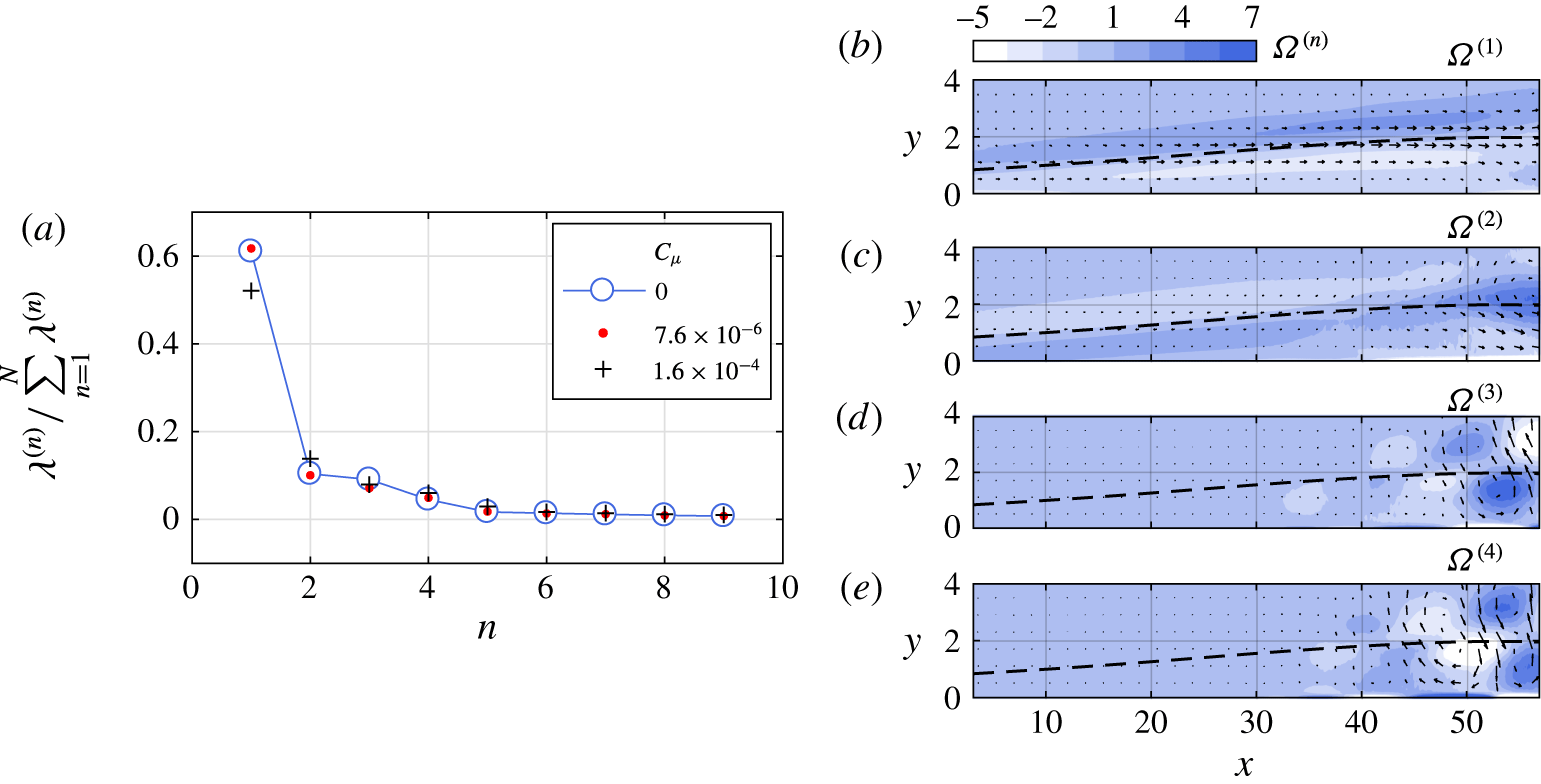
(a) Nine first POD eigenvalues for unforced and forced LSB. (b–e) Curl between the streamwise and wall-normal component of the first four eigenfunctions,
 $\unicode[STIX]{x1D6FA}^{(n)}=\unicode[STIX]{x1D735}\times (\unicode[STIX]{x1D6F7}_{u}^{(n)},\unicode[STIX]{x1D6F7}_{v}^{(n)})$
for
 $C_{\unicode[STIX]{x1D707}}=1.6\times 10^{-4}$
. Dashed line: displacement thickness.

The analysis shows that for both unforced and forced cases studied here, 85 % of the total estimated modal energy is concentrated within the first four POD modes (figure 5
a). A preliminary study sought to identify the underlying phenomena that each of the first four modes represent. In the unforced scenario,
 $\unicode[STIX]{x1D731}^{(1)}$
captures fluctuations of the shear layer attributed to the flapping behaviour. The following eigenfunctions,
 $\unicode[STIX]{x1D731}^{(2)}$
and
 $\unicode[STIX]{x1D731}^{(3)}$
represent the convective shedding of the LSB. Similar observations regarding the first three modes have been made by Lengani et al. (Reference Lengani, Simoni, Ubaldi and Zunino2014). When the bubble is forced (figure 5
b–e),
 $\unicode[STIX]{x1D731}^{(1)}$
remains associated with the shear layer flapping while the second eigenfunction,
 $\unicode[STIX]{x1D731}^{(2)}$
represents the rapid shrinkage and recovery of the LSB shear layer that is later described in § 5.1. Shedding and convection of the introduced disturbance are simultaneously captured in
 $\unicode[STIX]{x1D731}^{(3)}$
and
 $\unicode[STIX]{x1D731}^{(4)}$
, as they assume the same frequency.
3.4 Wavelet analysis
An in-depth overview of wavelet analysis may be found in the work of Daubechies (Reference Daubechies1992), thus, only the essential concepts are herein mentioned. In contrast to the discrete Fourier transform, the wavelet transform is suitable for capturing the spectral content of an arbitrary temporal signal,
 $\tilde{u} (\tilde{t})$
, such as the impulsive disturbance pertinent to this study. First, a baseline wavelet function,
 $\unicode[STIX]{x1D713}$
, must be chosen having zero mean and being localised in both time and frequency space. For this study, the Morlet wavelet is selected, expressed as
 $$\begin{eqnarray}\unicode[STIX]{x1D713}=\text{e}^{-(\tilde{t}/\tilde{c})^{2}}\text{e}^{\text{i}2\unicode[STIX]{x03C0}\tilde{f}_{c}\tilde{t}}.\end{eqnarray}$$
In order to satisfy the wavelet admissibility condition described by Farge (Reference Farge1992), the wavelet central angular frequency is selected to be
 $2\unicode[STIX]{x03C0}\tilde{f}_{c}=5~\text{rad}~\text{s}^{-1}$
while the damping parameter is
 $\tilde{c}=2~\text{s}$
.
Wavelet coefficients,
 $w$
, can then be estimated via
 $$\begin{eqnarray}w=\frac{\tilde{s}^{-1/2}}{\sqrt{2\unicode[STIX]{x03C0}\tilde{f}_{a}}}\int _{-\infty }^{\infty }\unicode[STIX]{x1D713}^{\ast }\left(\frac{\tilde{t}-\tilde{\unicode[STIX]{x1D70F}}}{\tilde{s}}\right)\tilde{u} (\tilde{t})\,\text{d}\tilde{t},\end{eqnarray}$$
which represents the convolution between the examined temporal signal,
 $\tilde{u} (\tilde{t})$
, and the translated and dilated complex conjugate of
 $\unicode[STIX]{x1D713}$
, denoted as
 $\unicode[STIX]{x1D713}^{\ast }$
. Here, translation and dilation scales of
 $\unicode[STIX]{x1D713}$
are represented by the terms
 $\unicode[STIX]{x1D70F}$
and
 $s$
respectively. In order to obtain unit power per scale,
 $w$
is scaled by
 $\sqrt{2\unicode[STIX]{x03C0}\tilde{f}_{a}}$
, with
 $\tilde{f}_{a}$
being the temporal signal sampling frequency.
4 The unforced LSB
4.1 Statistical features
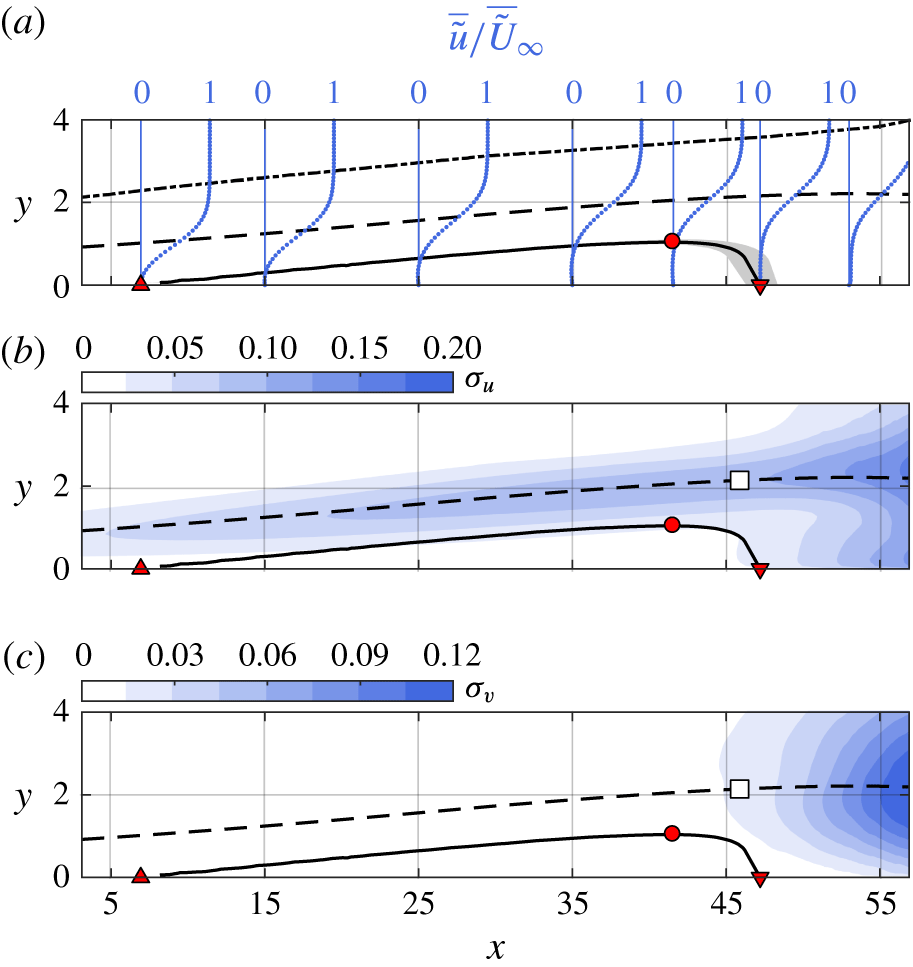
Prior to the analysis of the spatio-temporal response of the bubble to the impulsive forcing, it is instructive to examine the behaviour pertaining to the natural, unforced flow serving as baseline in this study. Figure 6 depicts time-averaged and fluctuating fields of the unforced flow. Driven by the adverse pressure gradient, the flow separates and reattaches downstream forming a closed, in the time-averaged sense, laminar separation bubble. The boundary of the LSB is defined by the mean dividing streamline, where the streamfunction
 $\unicode[STIX]{x1D713}=0$
. The mean separation and reattachment points are estimated at
 $\bar{x}_{s}=6.3$
and
 $\bar{x}_{r}=47.5$
, establishing a bubble length of
 $\bar{l}_{b}=41.2$
. The height of the bubble is defined as the point of the dividing streamline that is most distant from the wall,
 $\bar{h}=0.73$
, and is located at
 $\bar{x}_{h}=41.7$
. The maximum reverse flow observed within the bubble is of the order of
 $2\,\%$
of the local free stream velocity, indicating development of only convective instabilities as suggested by Gaster (Reference Gaster1992), Alam & Sandham (Reference Alam and Sandham2000) and Rist & Maucher (Reference Rist and Maucher2002).
Unforced LSB. (a) Time-averaged streamwise velocity profiles, scaled with the local free stream velocity. (b) Streamwise velocity fluctuations. (c) Wall-normal velocity fluctuations. Solid line: dividing streamline, dashed line: displacement thickness, dash-dotted line:
 $\unicode[STIX]{x1D6FF}_{99\,\%}$
. ▵: separation point, ▿: reattachment point, ○: maximum height, ▫: maximum shape factor. Shaded region: dividing streamline uncertainty limits for
 $\tilde{f_{a}}=$
500 Hz (see § 2.3).

Time-averaged streamwise velocity profiles scaled with the local free stream velocity (
 $\tilde{U} _{\infty }$
) are provided for several streamwise stations in figure 6(a). These profiles are similar to the hyperbolic tangent approximations suggested by Dovgal et al. (Reference Dovgal, Kozlov and Michalke1994) as well as with hot-wire measured profiles rectified in proximity to the wall (Niew Reference Niew1993; Watmuff Reference Watmuff1999; Diwan & Ramesh Reference Diwan and Ramesh2009). Similar to the studies of Gaster & Grant (Reference Gaster and Grant1975) and Marxen & Henningson (Reference Marxen and Henningson2011), reattachment is turbulent, however, there is no correspondence with a fully developed turbulent velocity profile (log-law) in the downstream vicinity of the reattachment. Indeed, as Alam & Sandham (Reference Alam and Sandham2000) indicate, relaxation of the boundary layer to a fully turbulent equilibrium state may require several bubble lengths, well downstream of the current field of view.
Fluctuations in the velocity field are quantified by the standard deviation of the two velocity components,
 $\unicode[STIX]{x1D70E}_{u}=\tilde{\unicode[STIX]{x1D70E}}_{u}/U_{0}$
and
 $\unicode[STIX]{x1D70E}_{v}=\tilde{\unicode[STIX]{x1D70E}}_{v}/U_{0}$
(figure 6
b,c). Two regions of increased fluctuation can be identified, the first extending along the displacement thickness, upstream of
 $\bar{x}_{h}$
. In this region, small variations in the shear layer distance from the wall due to the flapping mechanism (Zaman et al.
Reference Zaman, McKinzie and Rumsey1989) result in substantial changes of
 $u$
. Flapping does not affect the wall-normal velocity to the same extent, thus this region is absent in the
 $\unicode[STIX]{x1D70E}_{v}$
field. In contrast, the second region of elevated fluctuations is evident in both standard deviation fields downstream of
 $\bar{x}_{h}$
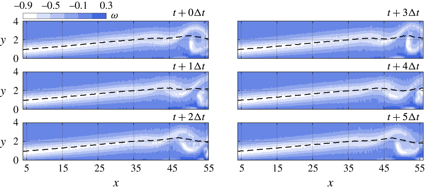
. Here, fluctuations are attributed to coherent vortex shedding (figure 7) and the subsequent breakdown to turbulence. In both velocity components, the associated velocity fluctuations are concentrated about the displacement thickness, known to approximate the trajectory of the shed structures (e.g. Boutilier & Yarusevych Reference Boutilier and Yarusevych2012).
Instantaneous vorticity demonstrating coherent vortex shedding at time steps separated by
 $\unicode[STIX]{x0394}t=5\tilde{f}_{p}/\tilde{f}_{a}$
, with
 $\tilde{f}_{a}=2~\text{kHz}$
. Dashed line: displacement thickness
 $(\unicode[STIX]{x1D6FF}^{\ast })$
.

4.2 Spectral content and stability characteristics
The global displacement of the separated shear layer in a LSB, i.e. flapping, is known to occur at significantly lower frequencies than the respective vortex roll up and shedding (e.g. Hain et al.
Reference Hain, Kähler and Radespiel2009). To access the spectral content of the shear layer flapping and vortex shedding of the unforced LSB, velocity measurements are performed at
 $\tilde{f}_{a}=250~\text{Hz}$
and
 $\tilde{f}_{a}=2000~\text{Hz}$
respectively. The selection of reference locations is made based on results in figure 6. For assessing flapping, a temporal signal,
 $u(t)$
is extracted at the streamwise location corresponding to the mean separation point,
 $\bar{x}_{s}$
, and at wall-normal location corresponding to
 $\unicode[STIX]{x1D6FF}^{\ast }(\bar{x}_{s})$
. Here, minimal vortex shedding signature is expected in the spectra. For characterising vortex shedding in the aft part of the bubble, a
 $v(t)$
signal is sampled at the streamwise location of mean maximum height and wall-normal distance equal to the displacement thickness
 $\unicode[STIX]{x1D6FF}^{\ast }(\bar{x}_{h})$
. Power spectral density is estimated via the Welch method (Welch Reference Welch1967) by dividing the corresponding temporal signal into 6 windows with 50 % overlap. The resulting frequency resolution is
 $St=3.6\times 10^{-5}$
and
 $2.8\times 10^{-4}$
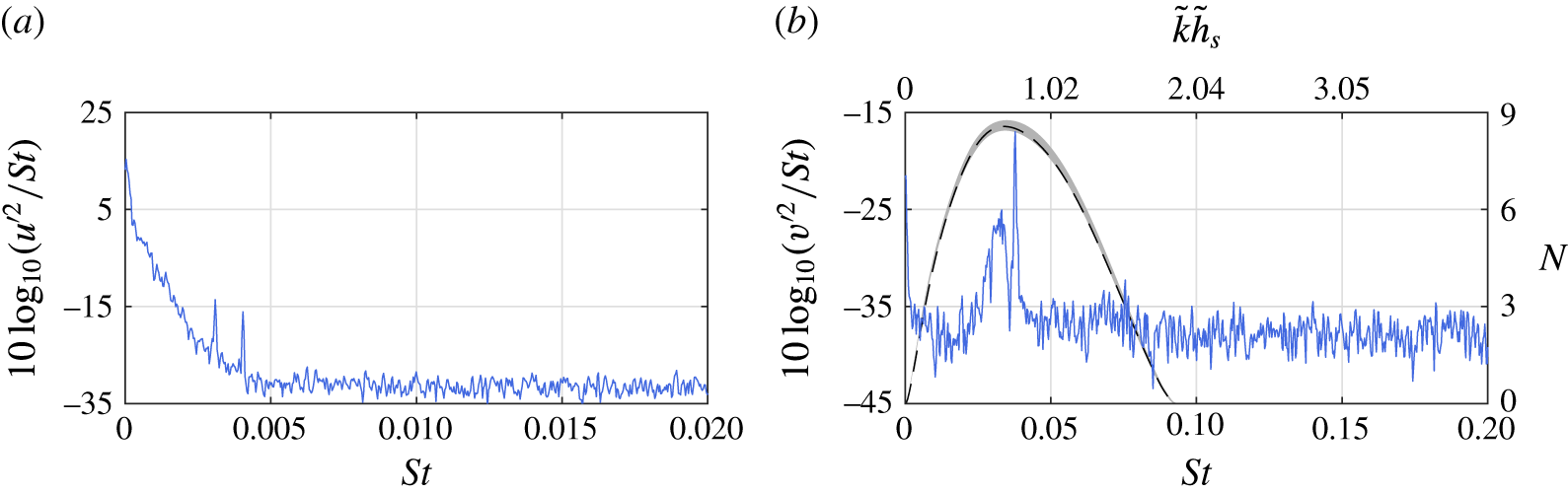
(0.13 and 0.98 Hz) for each of the two acquisition frequencies, respectively. The results shown in figure 8(a) suggest that flapping is comprised of a range of frequencies below
 $St=0.005$
(18 Hz). The two peaks present in the vicinity of
 $St\approx 0.005$
are attributed to aliasing from shedding signature and are approximately three orders of magnitude weaker than the highest point in the band. In contrast, shedding in the aft portion of the bubble produces a well-defined, elevated spectral content situated between
 $St=0.022$
(80 Hz) and
 $St=0.047$
(170 Hz) (figure 8
b). The most dominant frequency is
 $St=0.038$
(136 Hz), with an order of magnitude higher spectral density than the rest of the band. The spectral content is also related to the dimensionless shedding parameter,
 $\tilde{k}\tilde{h}_{s}$
(Yang & Voke Reference Yang and Voke2001). Here,
 $\tilde{k}=2\unicode[STIX]{x03C0}\tilde{f}/\tilde{u} _{infl}$
, is the angular wavenumber, with
 $\tilde{u} _{infl}$
being the inflection point velocity at
 $\bar{x}_{h}$
while
 $\tilde{h}_{s}$
is the shear layer thickness, equal to the displacement thickness at the same location. For the dominant shedding frequency,
 $\tilde{k}\tilde{h}_{s}=0.78$
, lying well within the expected limits for Kelvin–Helmholtz instability (
 $0<\tilde{k}\tilde{h}_{s}<1.2785$
, Yang & Voke Reference Yang and Voke2001). Furthermore, this is in good agreement with other relevant studies, e.g. Häggmark et al. (Reference Häggmark, Hildings and Henningson2001) and Simoni et al. (Reference Simoni, Ubaldi, Zunino, Lengani and Bertini2012b
).
Power spectral density of the unforced LSB. (a)
 $u(t)$
at
 $x=\bar{x}_{s}$
and
 $y=\unicode[STIX]{x1D6FF}^{\ast }(\bar{x}_{s})$
,
 $\tilde{f}_{a}=250~\text{Hz}$
. (b)
 $v(t)$
at
 $x=\bar{x}_{h}$
and
 $y=\unicode[STIX]{x1D6FF}^{\ast }(\bar{x}_{h})$
,
 $\tilde{f}_{a}=2000~\text{Hz}$
. Dashed line:
 $N$
factor at the same location. Shaded region:
 $N$
factor uncertainty at
 $\tilde{f_{a}}=$
500 Hz (see § 2.3).

In addition to spectral measurements, LST analysis is instrumental for identifying the dynamic characteristics relevant to the growth of instabilities in the separated shear layer. For validation purposes, a comparison between spectral results and
 $N$
factors computed from LST analysis is shown in figure 8(b). It can be seen that the frequencies associated with maximum amplification factor are in excellent agreement with that of the dominant peak in the spectrum, both corresponding to
 $St=0.038$
(136 Hz). The results of linear stability calculations (§ 3.2) performed on the time-averaged streamwise velocity field (figure 6
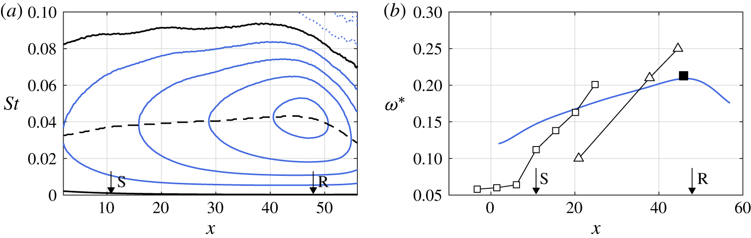
a) are presented in figure 9(a). It is evident that the growth rate of the most unstable frequency wave increases from
 $St=0.033$
(117 Hz) in the vicinity of separation to a maximum
 $St=0.043$
(155 Hz) near the mean maximum height
 $(x=42.3)$
. The corresponding amplification factor at this streamwise location is
 $N=7.2$
, comparable to the direct numerical simulations of Marxen et al. (Reference Marxen, Lang, Rist, Levin and Henningson2009). Moreover, LST calculations yield a convective speed of disturbances in the unforced LSB of approximately
 $0.45\tilde{U} _{0}$
. This is in good agreement with observations on the propagation of coherent vortex shedding structures (figure 7).
Unforced LSB stability diagram. (a) Non-dimensional growth rate,
 $-\unicode[STIX]{x1D6FC}_{i}=-\tilde{\unicode[STIX]{x1D6FC}}_{i}\tilde{\unicode[STIX]{x1D6FF}}^{\ast }$
in steps of 0.1. Solid lines:
 $-\unicode[STIX]{x1D6FC}_{i}\geqslant 0$
, dotted lines:
 $-\unicode[STIX]{x1D6FC}_{i}<0$
, dashed line: maximum
 $-\unicode[STIX]{x1D6FC}_{i}$
. (b) Dimensionless frequency
 $\unicode[STIX]{x1D714}^{\ast }=0.25\unicode[STIX]{x1D6FF}_{w}(2\unicode[STIX]{x03C0}\tilde{f})/\bar{U}$
. Solid line:
 $\unicode[STIX]{x1D714}^{\ast }$
estimated on the most unstable LST frequency. ▪:
 $\unicode[STIX]{x1D714}^{\ast }$
with
 $\tilde{f}$
derived from experimental velocity spectra at the maximum
 $\unicode[STIX]{x1D6FF}^{\ast }$
. ▵:
 $\unicode[STIX]{x1D714}^{\ast }$
from Watmuff (Reference Watmuff1999); ▫:
 $\unicode[STIX]{x1D714}^{\ast }$
from Diwan & Ramesh (Reference Diwan and Ramesh2009). For comparing datasets, their
 $x$
axis is scaled such that separation and reattachment locations match with the current experiment.

Monkewitz & Huerre (Reference Monkewitz and Huerre1982) suggested a scaling scheme for determining the occurrence of Kelvin–Helmholtz instability in free shear layers. Shear layers are characterised by an external and an internal velocity,
 $U_{e}$
and
 $U_{i}$
, respectively. Their difference,
 $\unicode[STIX]{x0394}U=U_{e}-U_{i}$
, is used for calculating the vorticity thickness,
 $\unicode[STIX]{x1D6FF}_{w}=\unicode[STIX]{x0394}U/(\unicode[STIX]{x2202}\bar{u}/\unicode[STIX]{x2202}y)_{max}$
. By including the dimensional frequency,
 $\tilde{f}$
, and the average of the bounding velocities,
 $\bar{U}=(U_{e}+U_{i})/2$
, a dimensionless frequency is expressed as
 $\unicode[STIX]{x1D714}^{\ast }=0.25\unicode[STIX]{x1D6FF}_{w}(2\unicode[STIX]{x03C0}\tilde{f})/\bar{U}$
. Monkewitz & Huerre (Reference Monkewitz and Huerre1982) demonstrated that the range of frequencies for Kelvin–Helmholtz instability lies in the interval
 $0.21<\unicode[STIX]{x1D714}^{\ast }<0.222$
. For the case of laminar separation bubbles, the internal velocity may be assumed negligible
 $(U_{i}\approx 0)$
while the external velocity is equal to the local free stream
 $(U_{i}\approx U_{\infty })$
. Since the distance of the bubble shear layer from the wall varies with respect to streamwise position, the aforementioned scaling is not valid unless the shear layer is at sufficient distance from the wall. Consequently, correspondence with the expected range
 $(\unicode[STIX]{x1D714}^{\ast }\approx 0.21)$
is mainly achieved in the region of the mean maximum height (e.g. Pauley et al.
Reference Pauley, Moin and Reynolds1990; Watmuff Reference Watmuff1999; Simoni et al.
Reference Simoni, Ubaldi, Zunino and Bertini2012a
). Figure 9(b) depicts a comparison between
 $\unicode[STIX]{x1D714}^{\ast }$
from the present results and the reporting of Watmuff (Reference Watmuff1999) and Diwan & Ramesh (Reference Diwan and Ramesh2009). The solid line corresponding to
 $\unicode[STIX]{x1D714}^{\ast }$
estimated based on the local most unstable frequency (dashed line in figure 9
a). Its maximum
 $(\unicode[STIX]{x1D714}^{\ast }=0.213)$
, agrees well with the estimate based on the dominant frequency in velocity spectra at the maximum
 $\unicode[STIX]{x1D6FF}^{\ast }$
 $(\unicode[STIX]{x1D714}^{\ast }=0.209)$
. Similar to the aforementioned references,
 $\unicode[STIX]{x1D714}^{\ast }$
exhibits linear increase downstream the separation point, confirming the inviscid nature of disturbance amplification (Watmuff Reference Watmuff1999). The differences between the slopes of the linear portions of the three datasets are attributed to the substantially different bubble height to length ratio between the respective experiments.
5 The forced LSB
The LSB is subjected to impulsive forcing with amplitudes ranging from
 $C_{\unicode[STIX]{x1D707}}=1.5\times 10^{-6}$
to
 $C_{\unicode[STIX]{x1D707}}=1.6\times 10^{-4}$
. The pulses are repeated at a frequency of
 $\tilde{f}_{p}=2$
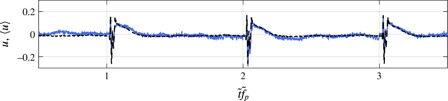
Hz. Sample temporal and phase-averaged streamwise velocity signals at the mean maximum height of the unforced LSB are provided in figure 10. The beginning of each cycle is marked by introduction of a pulse and is identified as the vertical grid line. The results illustrate the dynamic nature of the cycle, confirming that the transient completely subsides before the introduction of the next impulse. The strong cycle-to-cycle periodicity affirms the feasibility of phase averaging for subsequent increase of statistical significance. Experimental limitations dictate that, for each acquisition frequency (250 Hz, 500 Hz and 2000 Hz), the number of realisations available at each phase is 87, 43 and 10, respectively.
Sample of velocity signal at the location of maximum height,
 $\bar{h}$
, for
 $C_{\unicode[STIX]{x1D707}}=1.6\times 10^{-4}$
. The initiation of each forcing cycle is marked by the vertical grid lines. Solid line: raw velocity signal,
 $u$
. Dashed line: phase-averaged velocity signal,
 $\langle u\rangle$
.

5.1 Temporal response to impulse
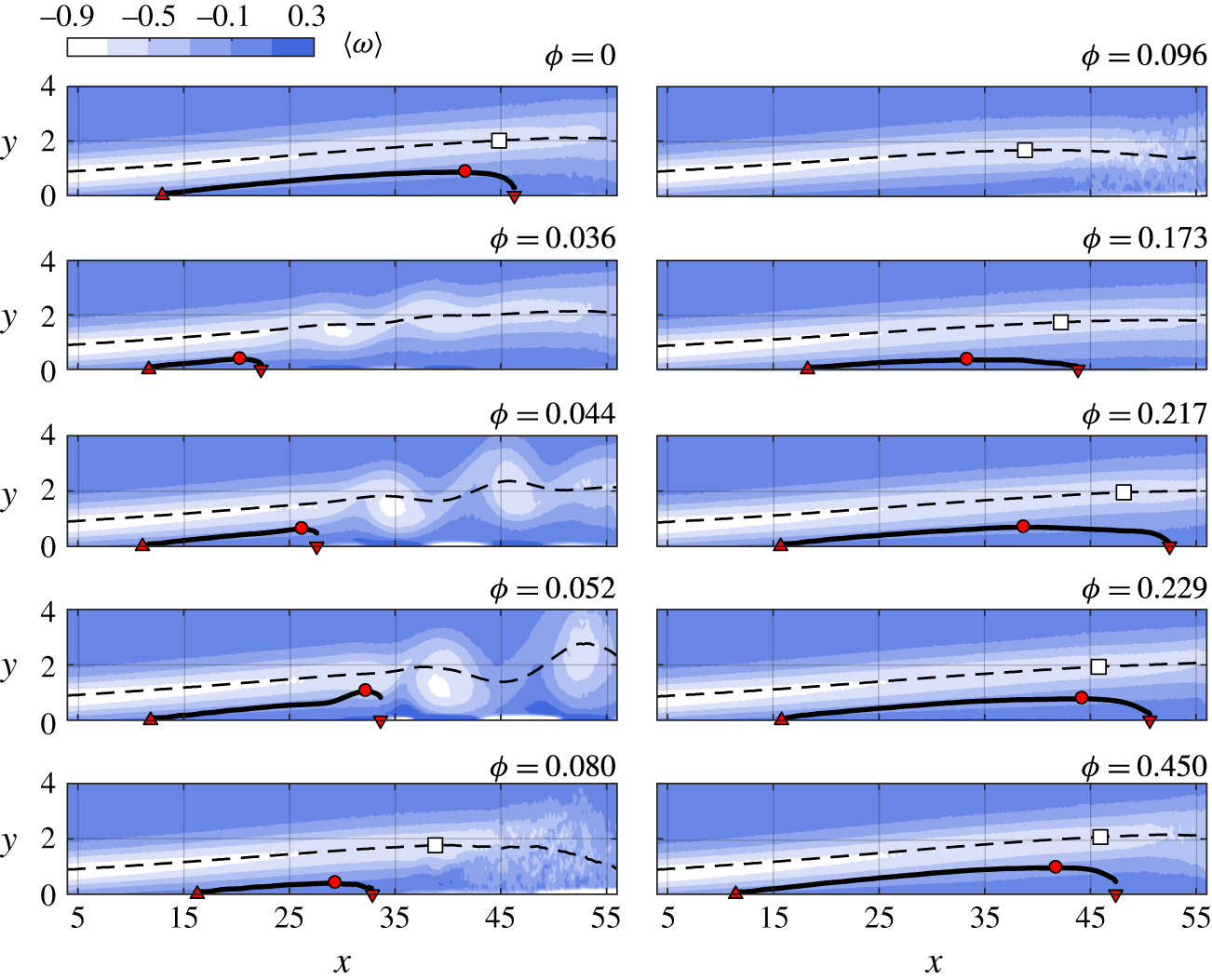
Phase-averaged vorticity within the forcing cycle for
 $C_{\unicode[STIX]{x1D707}}=5.4\times 10^{-5}$
. Solid line: dividing streamline; dashed line: displacement thickness
 $(\unicode[STIX]{x1D6FF}^{\ast })$
; ▵: separation point; ▿: reattachment point; ○: maximum height; ▫: location of maximum shape factor.

The pertinent features of the temporal response of the LSB to the impulsive forcing are captured by phase-averaged vorticity fields,
 $\langle \unicode[STIX]{x1D714}\rangle =\langle \tilde{\unicode[STIX]{x1D714}}\rangle \tilde{\unicode[STIX]{x1D6FF}}_{s_{0}}^{\ast }/\tilde{U} _{0}$
, shown in figure 11. An animated sequence of the ensuing events is provided as a supplementary movie, available at https://doi.org/10.1017/jfm.2017.217. The forcing magnitude of the demonstrated sequence is
 $C_{\unicode[STIX]{x1D707}}=5.4\times 10^{-5}$
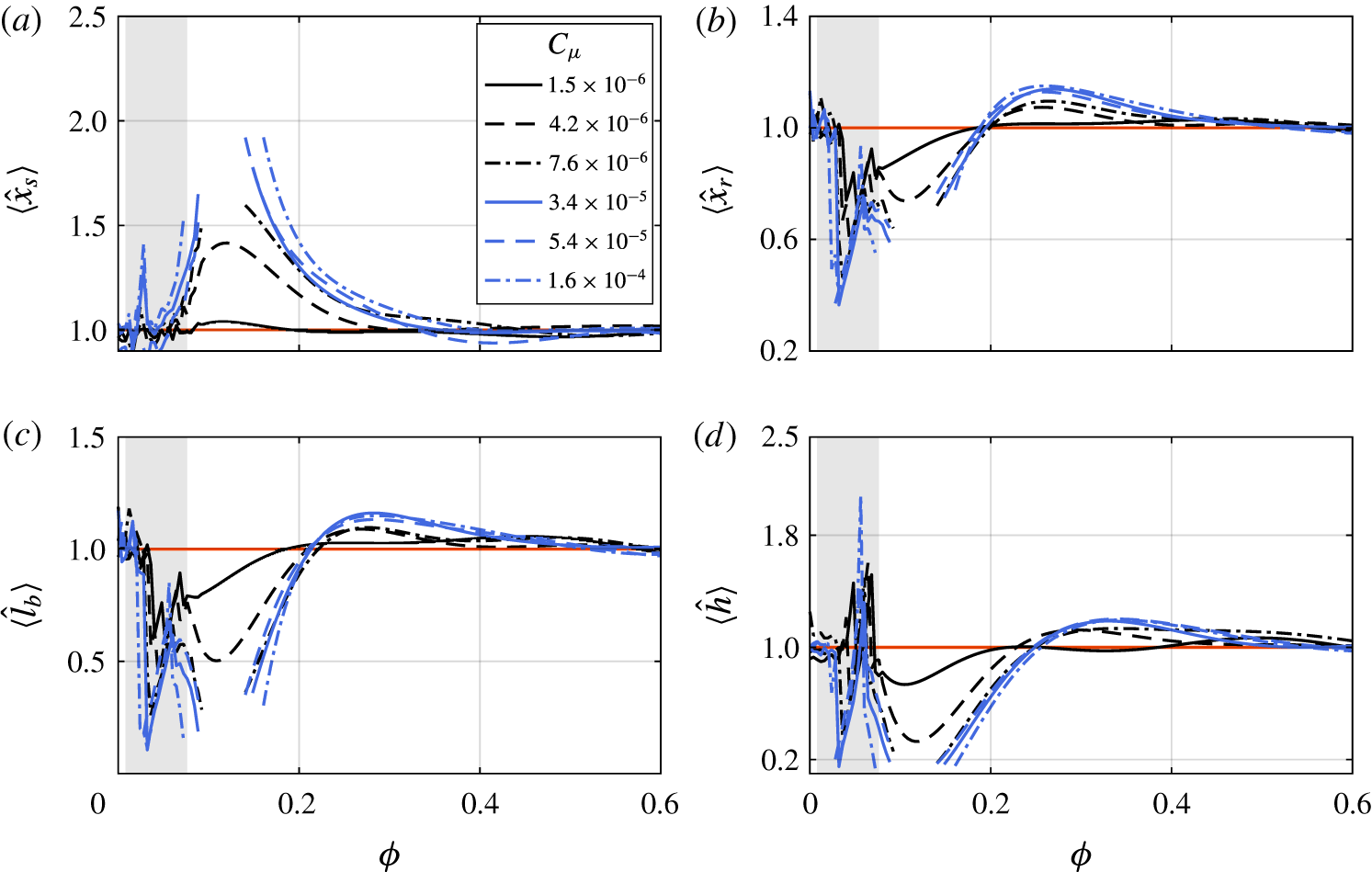
, although the same general behaviour has been observed at all other forcing amplitudes. An overview of the topological changes of the separation bubble for all forcing amplitudes is achieved by tracing bounding properties of the LSB with respect to phase and is shown in figure 12. Specifically, the phase-averaged location of separation,
 $\langle x_{s}\rangle$
and reattachment,
 $\langle x_{r}\rangle$
, bubble length,
 $\langle l\rangle =\langle x_{r}\rangle -\langle x_{s}\rangle$
, and maximum height,
 $\langle h\rangle$
are shown in figure 12. For ease of comparison, these metrics are normalised by the corresponding parameters of the unforced LSB (thus are denoted with the hat symbol). At this point a note needs to be made considering the definition of the LSB boundaries. As seen in figure 11, for phases
 $\unicode[STIX]{x1D719}<0.08$
, the introduced vortical wave packet distorts the flow to a degree where a classical definition of LSB is no longer applicable. As such, the focus of the analysis is directed to phases greater than 0.08. In figure 12, the shaded area corresponds indeed to phases at which the introduced disturbance advances within the field of view.
Shortly after the introduction of the pulse, a wave packet emerges, which develops into a set of corotating vortices that propagate downstream (
 $0.036<\unicode[STIX]{x1D719}<0.052$
, figure 11). The convective nature of the developing disturbance confirms the aforementioned assumption of global stability of the present LSB, based on the magnitude of maximum reverse flow of 2 % (Gaster Reference Gaster1992; Alam & Sandham Reference Alam and Sandham2000). Once the developing wave packet convects past the streamwise location of the mean maximum height of the unforced case
 $(\unicode[STIX]{x1D719}=0.08)$
, the LSB undergoes rapid contraction with the separation and reattachment points shifting downstream and upstream respectively, similar to the DNS observations of Rist & Maucher (Reference Rist and Maucher2002). For forcing amplitudes exceeding
 $C_{\unicode[STIX]{x1D707}}=4.2\times 10^{-6}$
, the LSB is completely eliminated (
 $\unicode[STIX]{x1D719}=0.096$
, figure 11). Complete elimination of the LSB is signified in figure 12 by discontinuities in the plots at phases close to
 $\unicode[STIX]{x1D719}=0.1$
. Within the same range, the two lowest forcing amplitudes result in the reduction of LSB size, albeit not complete elimination. From this point, the LSB starts recovering, a process that is significantly slower than the contraction. Growth of the LSB is also occurring towards both upstream and downstream directions (figure 12).
Evolution of phase-averaged (a) separation point; (b) reattachment point; (c) bubble length and; (d) maximum bubble height. All metrics are scaled with the respective unforced value. Shaded region: interval during which the wave packet is within the field of view.

During the recovery stage, the LSB elongates before contracting to its unperturbed state (
 $\unicode[STIX]{x1D719}\approx 0.45$
, figure 11). The reattachment point shifts downstream, similar to the behaviour of the bursting process described by Gaster (Reference Gaster1967) and Marxen & Henningson (Reference Marxen and Henningson2011). This produces the overshoot in the reattachment location, bubble length and the maximum height seen in figures 12(b), 12(c) and 12(d), respectively, within
 $0.2<\unicode[STIX]{x1D719}<0.4$
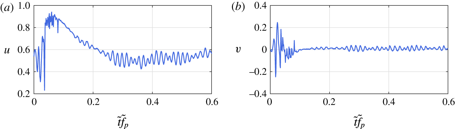
. Bursting is accompanied by reduction of the vortex shedding strength. This is visualised in figure 13, which depicts instantaneous velocity traces probed at the aft part of the bubble. At the early stages of the bursting process, for a short time interval after the bubble elimination, no shedding traces are evident within the field of view
 $(0.1<\tilde{t}\tilde{f}<0.15)$
. Shedding, however, quickly resumes as the bubble grows, albeit at a lower strength, until reattachment assumes its most downstream location (
 $\unicode[STIX]{x1D719}\approx 0.25$
, figure 11). From this point, the bubble height increases further than its unforced value, an inertial effect that is a direct consequence of the vortex shedding strength reduction. More specifically, mass accumulation caused by the reverse flow is not balanced by sufficient mass entrainment in the aft portion through vortex shedding until breakdown has moved sufficiently upstream. After the latter occurs, the LSB finally recovers to its unperturbed state.
The dynamic cycle described here, including the bubble size reduction or elimination, is also observed in cases where laminar separation bubbles interact with controlled periodic wake disturbances (e.g. Simoni et al. Reference Simoni, Ubaldi, Zunino and Bertini2012a ). In addition, the separation bubble does not exhibit any features of long bubbles (Marxen & Henningson Reference Marxen and Henningson2011) throughout the forcing cycle, thus the elongation represents part of a dynamic process of a short bubble.
Velocity signals at
 $x=55$
and
 $y=\bar{\unicode[STIX]{x1D6FF}}_{0}^{\ast }(55)$
for
 $C_{\unicode[STIX]{x1D707}}=5.4\times 10^{-5}$
. (a) Streamwise component,
 $u$
. (b) Wall-normal component,
 $v$
.

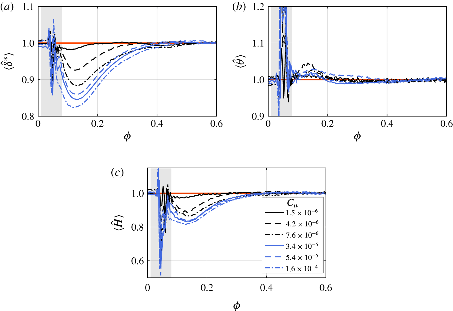
The LSB topology is dependent on the laminar to turbulent transition process as the latter governs momentum entrainment and leads to reattachment. It is therefore expected that variations in laminar to turbulent transition within the LSB shear layer are accompanied by evident changes in integral boundary layer length scales (van Ingen Reference van Ingen2008; Yarusevych & Kotsonis Reference Yarusevych and Kotsonis2017). The aforementioned quantities are estimated during the forcing cycle at the streamwise location of the unforced LSB mean maximum height and are shown in figure 14. It is evident that during bursting, increasing forcing amplitude results in decrease of displacement thickness (
 $\unicode[STIX]{x1D6FF}^{\ast }$
) and increase of momentum thickness (
 $\unicode[STIX]{x1D703}$
). Consequently, the shape factor (
 $H=\unicode[STIX]{x1D6FF}^{\ast }/\unicode[STIX]{x1D703}$
) decreases, signifying enhanced stabilisation of the boundary layer for increasing forcing amplitude, consistent with the documentations of Rist & Augustin (Reference Rist and Augustin2006) and Marxen & Rist (Reference Marxen and Rist2010).
Evolution of phase-averaged boundary layer integral quantities scaled to the respective unforced value. Values are probed at the streamwise location of maximum height of the unforced LSB
 $\bar{x}_{h_{0}}$
. (a) Displacement thickness; (b) momentum thickness; (c) shape factor. Shaded region: interval during which forced disturbance is within the field of view.

Prior to the disturbance introduction (
 $\unicode[STIX]{x1D719}=0$
), the location of maximum shape factor,
 $H$
, is located in the upstream vicinity of the mean reattachment location (figures 14
c and 11). This location corresponds well to the abrupt rise of wall-normal velocity fluctuations in the unforced bubble (figure 6), signifying the onset of the shear layer breakdown. Due to the low turbulence environment and the strongly inflectional profiles exhibited by the LSB, the breakdown and transition onset locations are in close proximity. As such, a first-order estimation of the breakdown onset location can be derived based on the streamwise location where the shape factor is maximised. This is indicated by a square marker in figure 11. Shortly after the convection of the forced wave packet and the elimination of the LSB, the breakdown onset point swiftly shifts upstream by approximately
 $12\tilde{\unicode[STIX]{x1D6FF}}_{s}^{\ast }$
(
 $\unicode[STIX]{x1D719}=0.08$
and
 $0.096$
). Here, the absence of reverse flow leads to temporary stabilisation, which, in turn, causes the breakdown onset point to shift downstream
 $(\unicode[STIX]{x1D719}=0.173)$
. This downstream shift persists throughout the entire bursting process (figure 12). Given the observed behaviour, the phase at which the breakdown onset location is most downstream corresponds to the longest LSB (
 $\unicode[STIX]{x1D719}\approx 0.25$
), i.e. at the end of bursting (figure 12
c). As gradual recovery ensues after maximum elongation, the breakdown onset point propagates upstream, reaching its unforced location at
 $\unicode[STIX]{x1D719}\approx 0.5$
.
As mentioned earlier, during the interval between the bubble elimination and the end of the bursting process, the LSB shedding strength is reduced (figure 13). This notion, in conjunction with the significant changes in the breakdown onset location implies that an impulsive disturbance significantly influences the stability characteristics of the LSB. Following the elimination of the reverse flow region, the temporary stabilisation leads to reduced growth rate of incoming disturbances, thus, transition to turbulence and the associated increase of wall-normal mixing are driven to occur farther downstream. Consequently, the separated shear layer fails to reattach as early as in the unforced scenario. It is important to stress here that the apparent stabilisation of the LSB is slightly different than the one observed by Gaster (Reference Gaster1967) and Marxen & Henningson (Reference Marxen and Henningson2011) in their respective studies. While a combination of mean flow distortion and changing amplitude of incoming instabilities was at play in the aforementioned studies, the current investigation is performed with a non-changing incoming disturbance amplitude during the bubble bursting and recovery phase.
A final comment can be given on the characteristic time scales of the observed topological changes in the LSB. As indicated by
 $\langle {\hat{h}}\rangle$
in figure 12(d), increase of forcing amplitude results in faster elimination of the LSB as well as increase of the duration of reverse flow absence. Nonetheless, the phase at which the LSB recovers to its unperturbed state
 $(\unicode[STIX]{x1D719}\approx 0.45)$
seems to be independent of the forcing amplitude. This serves as an additional indication that while the rapid and significant changes imparted on the topology and shedding behaviour of the LSB are due to the initial effect of impulsive forcing, the recovery to the unperturbed state is driven by the global pressure gradient and the amplitude of the natural incoming disturbances, which are constant for all tested cases.
5.2 Quasi-steady spatial stability
According to the analysis carried out in § 4.2, LST predictions (figure 9) suggest that the most amplified instability mode in the unforced LSB manifests at a frequency of approximately
 $St=0.038$
(136 Hz,
 $\tilde{k}\tilde{h}_{s}=0.78$
). This is confirmed by the spectral content (figure 8) where the band of amplified frequencies ranges from
 $St=0.022$
(80 Hz,
 $\tilde{k}\tilde{h}_{s}=0.62$
) to
 $St=0.047$
(170 Hz,
 $\tilde{k}\tilde{h}_{s}=0.96$
). The results agree well with the findings of similar studies, e.g. Häggmark et al. (Reference Häggmark, Hildings and Henningson2001),
 $\tilde{k}\tilde{h}_{s}=0.88$
, Yang & Voke (Reference Yang and Voke2001),
 $\tilde{k}\tilde{h}_{s}=0.98$
and Simoni et al. (Reference Simoni, Ubaldi, Zunino, Lengani and Bertini2012b
),
 $\tilde{k}\tilde{h}_{s}=0.98$
. In addition, as demonstrated in § 5.1, the time interval from the disturbance introduction until full recovery of the LSB is approximately
 $\unicode[STIX]{x1D6FF}\unicode[STIX]{x1D719}=0.45$
, yielding an equivalent frequency of
 $St=1.2\times 10^{-3}$
(4.4 Hz). Due to this large separation of time scale between pertinent instability modes and global topology changes in the LSB, the forcing cycle may be treated as a quasi-steady process (Brevdo & Bridges Reference Brevdo and Bridges1997). In this manner, the statistical and stability properties at any given phase are considered independent of the rate of change of bubble characteristics.
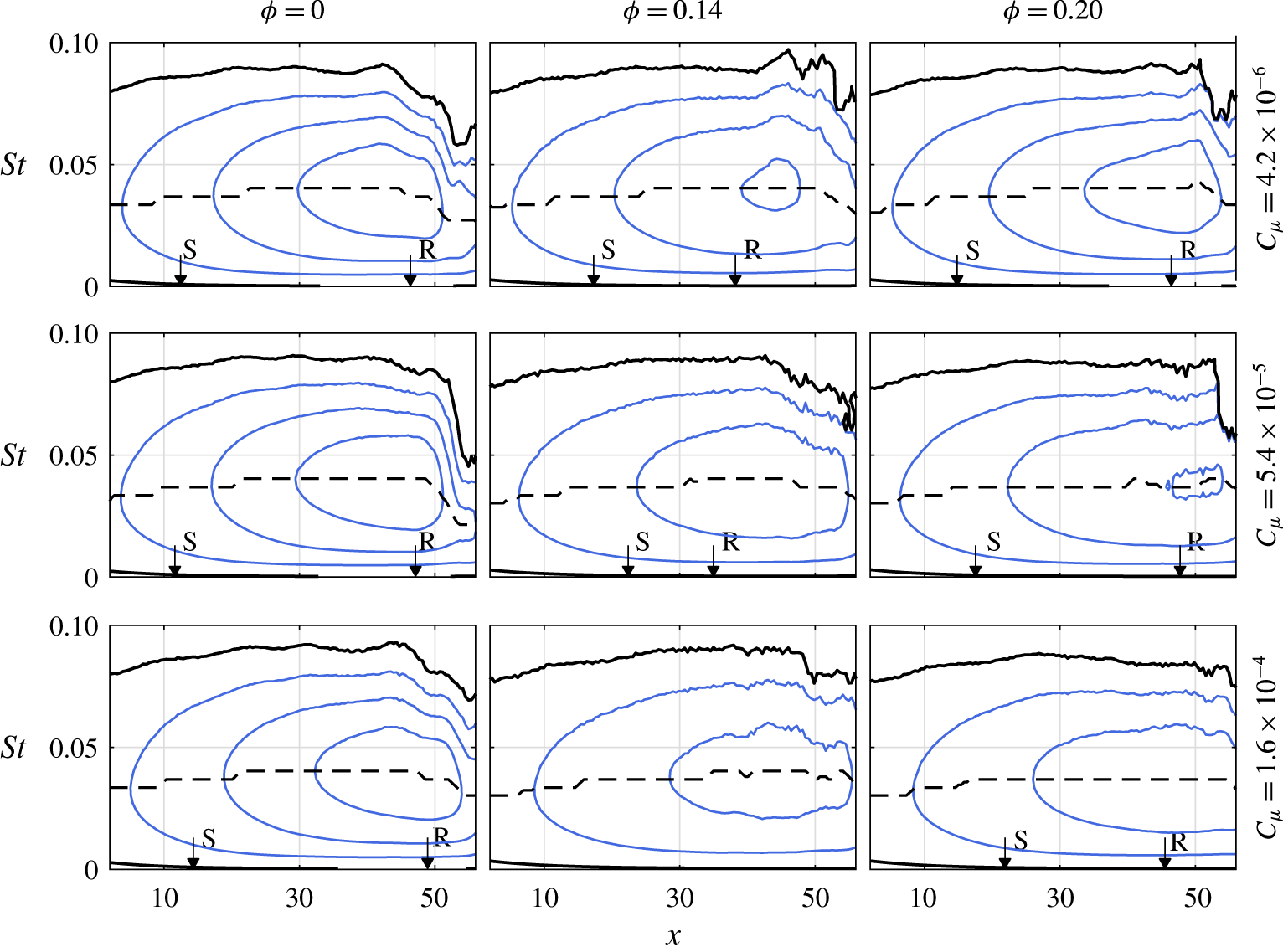
Stability diagrams for selected phases and forcing amplitudes. Iso-contours of non-dimensional growth rate,
 $-\unicode[STIX]{x1D6FC}_{i}=-\tilde{\unicode[STIX]{x1D6FC}}_{i}\tilde{\unicode[STIX]{x1D6FF}}^{\ast }$
, in steps of 0.1. Solid lines:
 $-\unicode[STIX]{x1D6FC}_{i}\geqslant 0$
, dashed line: frequency of the most unstable mode. Separation and reattachment points are noted with S and R, respectively.

The assumption of quasi-steady behaviour allows performing LST analysis as formulated in § 3.2, using phase-averaged streamwise velocity fields. Contours of growth rates for three different forcing amplitudes and selected phases within the forcing cycle are shown in figure 15. For
 $\unicode[STIX]{x1D719}=0$
, the growth rate fields correspond to the unforced case (figure 9
a). In the following column
 $(\unicode[STIX]{x1D719}=0.14)$
, the bubble attains its smallest size or is eliminated, depending on forcing amplitude. It is evident that the magnitude of the maximum growth rate decreases for increasing forcing amplitude, indicating increase of stability of the LSB, supporting observations made in § 5.1. Similar behaviour is observed for
 $\unicode[STIX]{x1D719}=0.20$
, during the recovery phase.
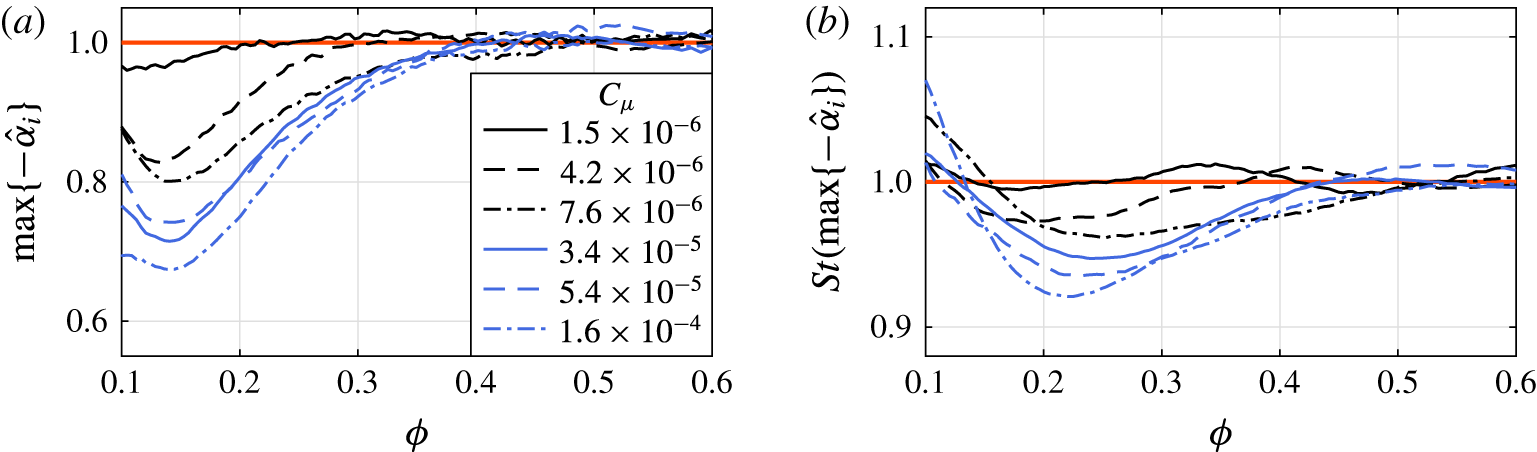
(a) Maximum growth rate and (b) most unstable frequency at
 $\bar{x}_{h_{0}}$
for different forcing amplitudes as predicted by quasi-steady LST analysis. Quantities are normalised with the respective unforced values.

The trend for different forcing amplitudes within the forcing cycle becomes more evident by plotting the maximum growth rate at the streamwise location of the unforced LSB mean maximum height,
 $\bar{x}_{h_{0}}$
, with respect to phase (figure 16
a). Here, with reference to figure 12, it is noted that as the LSB recovers
 $(\unicode[STIX]{x1D719}>0.2)$
growth rates are increasing. In addition, LST calculations indicate that the frequency of the most unstable mode at the same location (figure 16
b) decreases with respect to its unforced LSB value during the bubble recovery phase
 $(0.1<\unicode[STIX]{x1D719}<0.4)$
, with a minimum achieved at
 $\unicode[STIX]{x1D719}\approx 0.25$
. This reduction, however, is relatively small
 $({\approx}5\,\%)$
compared to the respective reduction of growth rate
 $({\approx}25\,\%)$
, agreeing well with observations of Marxen et al. (Reference Marxen, Kotapati, Mital and Zaki2015).
As evident by the previous discussion, the change in mean bubble size and topology has direct consequence on stability. Reduction of the bubble height and even complete elimination of the reverse flow region results in more stable flow in LST terms. Furthermore, the effect of impulsive forcing on the integral properties of the boundary layer, such as
 $\unicode[STIX]{x1D6FF}^{\ast }$
,
 $\unicode[STIX]{x1D703}$
and
 $H$
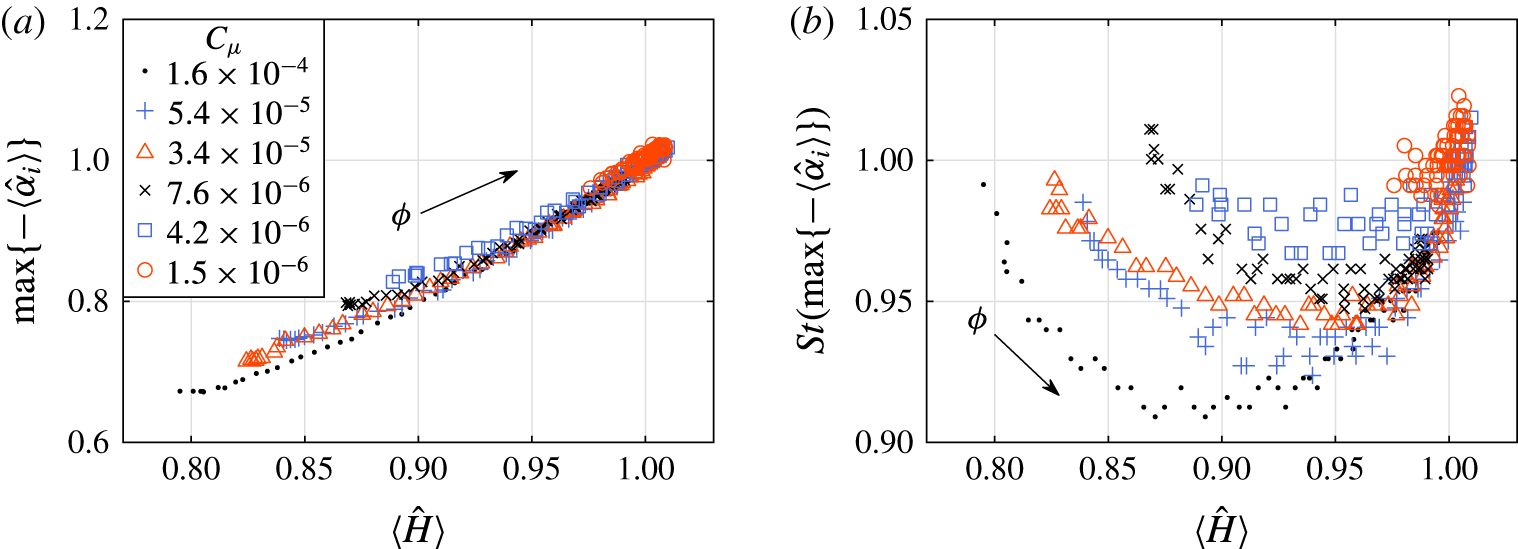
, appears to follow similar trend as the growth rate and frequency of most amplified mode (figure 14). The maximum growth rate as a function of the corresponding shape factor at
 $\bar{x}_{h_{0}}$
is, therefore, shown in figure 17(a) for all phases during the recovery phase of the forcing cycle
 $(0.1<\unicode[STIX]{x1D719}<0.5)$
and all forcing amplitudes. For ease of comparison the values are scaled with the respective values pertaining to the unforced bubble.
(a) Maximum growth rate and (b) most unstable frequency for different forcing amplitudes. Data are probed at
 $\bar{x}_{h_{0}}$
and
 $0.1<\unicode[STIX]{x1D719}<0.5$
as a function of the local shape factor. All quantities are normalised with the respective unforced values.

It is apparent that all growth rates collapse on a monotonic, nearly linear regression. This indicates strong correlation between stability of the LSB and integral characteristics of the boundary layer regardless of the forcing amplitude, as previously suggested in the works of LeBlanc, Blackwelder & Liebeck (Reference LeBlanc, Blackwelder and Liebeck1989), van Ingen & Kotsonis (Reference van Ingen and Kotsonis2011) and Boutilier & Yarusevych (Reference Boutilier and Yarusevych2012). The implication of this notion for both flapping and bursting mechanisms is a consequence of altered stability characteristics due to the influence of incoming perturbations on the bubble topology. If the perturbations are of small amplitude and intermittent, as in the case of free stream disturbances, the LSB will react with mild shape factor and stability variations leading to the observation of the flapping phenomenon. In turn, introduction of a periodic disturbance at the most unstable frequency or impulsive forcing, of amplitude higher than environmental disturbances, may achieve reduction of flapping by pegging the stability characteristics, explaining the observations of Dovgal & Boiko (Reference Dovgal, Boiko, Fasel and Saric1994). In the extreme case of a high amplitude impulsive disturbance, the flow distorts to an extent that the LSB diminishes and by consequence stabilises considerably. As a result, the shear layer breakdown onset location is forced downstream (see figure 11), alleviating mixing benefits, and resulting in bubble bursting. This confirms the observations of Marxen & Henningson (Reference Marxen and Henningson2011) regarding the bursting process based on simulations where the flow becomes more stable by decreasing the amplitude of numerical unsteady forcing.
Contrary to the growth rates, the frequency of the most unstable waves is not directly proportional to the shape factor but demonstrates a parabolic variation (figure 17
b). In particular, the minimum value is achieved at
 $\unicode[STIX]{x1D719}\approx 0.22$
. With reference to the trace of the bubble length and height shown in figure 12(c,d), this coincides with the instant when these quantities temporarily assume their unforced value, followed by the elongation due to bursting. The extremum in the frequency variation with shape factor suggests a notable change in the boundary layer characteristics. Indeed, the inflection point in the displacement thickness can be observed at the same time instant (
 $\unicode[STIX]{x1D719}\approx 0.22$
) in figure 14(a).
5.3 Disturbance characteristics
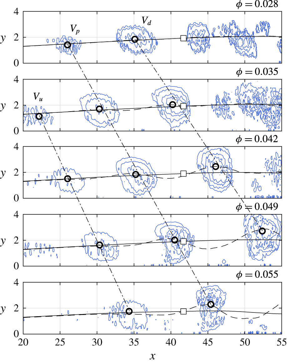
 $Q$
-criterion for
 $C_{\unicode[STIX]{x1D707}}=1.6\times 10^{-4}$
at various phases. Dashed lines: displacement thickness. Solid lines: displacement thickness based on reconstruction with
 $\unicode[STIX]{x1D731}^{(1)}$
and
 $\unicode[STIX]{x1D731}^{(2)}$
. Dash-dot lines: connect the vortex centroids (indicated by circles) at different time instants. Square marker: location of probe used for extracting signal for wavelet analysis (figure 19).

The analysis performed in the preceding sections demonstrates the strong influence of the impulsive disturbance on the LSB dynamic topology and stability. It is, therefore, imperative to describe and quantify the disturbance evolution in order to close the interaction loop. Complementary to figure 11, contours of
 $Q$
-criterion (Hunt, Wray & Moin Reference Hunt, Wray and Moin1988) are shown in figure 18 for
 $0.026<\unicode[STIX]{x1D719}<0.046$
. A set of three corotating vortices, labelled
 $V_{p}$
,
 $V_{u}$
and
 $V_{d}$
, dominates the flow field, downstream of which the
 $Q$
-criterion detects evidence of structures shed prior to the introduction of the impulse.
 $V_{p}$
is the primary vortex produced due to the introduction of the pulse as it can be traced to the streamwise location of the actuator,
 $x=0$
, at
 $\unicode[STIX]{x1D719}=0$
.
 $V_{d}$
is induced by
 $V_{p}$
shortly after the impulse and becomes measurable when
 $V_{p}$
has reached
 $x\approx 15$
. A tertiary weaker vortex,
 $V_{u}$
, emerges upstream of
 $V_{p}$
closing the cascade. The streamwise distance between all three vortices is initially approximately
 $9\unicode[STIX]{x1D6FF}_{s}^{\ast }$
, however, it gradually increases to
 $12\unicode[STIX]{x1D6FF}_{s}^{\ast }$
between
 $V_{p}$
and
 $V_{d}$
, as
 $V_{d}$
passes through the accelerated flow in the reattachment region. The process closely resembles the wave packet sequence observed by Watmuff (Reference Watmuff1999). For completing characterisation of this wave packet, analyses of its frequency, convective speed and growth rate are performed.
Due to the highly transient nature of events, assessment of the frequency characteristics of the disturbance cannot be performed via Fourier analysis. Instead, the wavelet transform is employed as described in § 3.4, on the phase-averaged vorticity signal. The disturbance is expected to affect the shape of the LSB as it convects, thus the probe location where vorticity is extracted takes into account the deformation of the separated shear layer. Specifically, the probe’s streamwise location is fixed to the location of mean maximum height of the unforced LSB, while the distance of the probe from the wall is set to the displacement thickness at the corresponding phase. In order to reduce the uncertainty in the probe location due to the passing wave packet disturbance, displacement thickness is estimated on reduced-order velocity fields, reconstructed by considering POD modes
 $\unicode[STIX]{x1D731}^{(1)}$
and
 $\unicode[STIX]{x1D731}^{(2)}$
. As demonstrated in § 3.3, these modes capture the overall motion of the bubble disregarding shedding as well as distortion of the shear layer due to the presence of the disturbance. A comparison between the displacement thickness calculated based on the full phase-averaged signal and the displacement thickness calculated on the reduced-order signal
 $(\unicode[STIX]{x1D6FF}_{ro}^{\ast })$
is shown in figure 18. The location of the probe coinciding with the reduced-order displacement thickness is indicated by the square marker. The extracted vorticity signal and the corresponding wavelet coefficients for forcing amplitude of
 $C_{\unicode[STIX]{x1D707}}=1.6\times 10^{-4}$
are plotted in figure 19. Peaks in the wavelet coefficient field indicate that the dominant frequency assumed by the wave packet is approximately
 $St=0.037$
(134 Hz), which agrees with the most amplified frequency of the unforced bubble, determined from velocity spectra and LST predictions at the same streamwise position (§ 4.2). It may be noted that the introduced disturbance frequency maintains approximately a constant value during all the phases for which it is detected.
(a) Signal of phase-averaged vorticity at
 $x=\bar{x}_{h}$
and
 $y=\langle \unicode[STIX]{x1D6FF}_{ro}^{\ast }\rangle$
for
 $C_{\unicode[STIX]{x1D707}}=1.6\times 10^{-4}$
. (b) Normalised wavelet coefficients. Dashed line: connects the maxima at each phase.

Though it is possible to obtain an approximation of the disturbance convective speed by tracing the propagation of the vortex cores (figure 18), a more reliable approach is followed based on integrating the phase-averaged wall-normal velocity component along the
 $y$
-direction. With this method, disturbance traces are detectable even at upstream locations where the structures are still too weak to be detected by vortex identification schemes. The result is shown in an
 $x-\unicode[STIX]{x1D719}$
diagram in figure 20(a), for the case corresponding to forcing amplitude of
 $C_{\unicode[STIX]{x1D707}}=1.6\times 10^{-4}$
. Two distinct sets of convective ridges are identified. The first set is located in the interval
 $0<\unicode[STIX]{x1D719}<0.08$
, spanning throughout the entire streamwise extent and pertaining to the passage of the three structures induced by the pulse (
 $V_{p}$
,
 $V_{d}$
and
 $V_{u}$
, figure 18). The second set of convective ridges (
 $\unicode[STIX]{x1D719}>0.2$
and
 $x>40$
) is the signature of the coherent vortex shedding in the aft part of the LSB, re-established after the bursting process. Between these two regions in time (
 $0.08<\unicode[STIX]{x1D719}<0.2$
), elimination of the LSB takes place, followed by cessation of vortex shedding associated to the bursting process (see also figure 13), therefore, no clear convective ridges are observed. The convective speed of the wave packet introduced by the impulsive forcing is directly related to the slope of the dominant convective ridge (marked by the dashed line in figure 20
a). The convective speed is found to be largely independent of the forcing amplitude (figure 20
b) with an average value of
 $0.46\tilde{U} _{0}$
, equal to estimations made on the unforced bubble (§ 4.2). This is in good agreement with LST analysis predictions as well as the work of Rist & Maucher (Reference Rist and Maucher2002) and Pröbsting & Yarusevych (Reference Pröbsting and Yarusevych2015).
(a) Phase–streamwise location map of
 $y$
-integral of wall-normal phase-averaged velocity
 $(\int \langle v\rangle \,\text{d}y)$
for
 $C_{\unicode[STIX]{x1D707}}=1.6\times 10^{-4}$
. (b) Convective speed (
 $u_{c}$
) of forced disturbance for tested forcing amplitudes. ○: measurements and ▫: corresponding LST predictions for the most unstable mode at
 $St=0.043$
(155 Hz).

Figure 20(a) provides an additional confirmation that the wave packet is convectively, rather than globally unstable due to the lack of ridges with negative slope that would otherwise signify upstream propagation of disturbances in the vicinity of the wall. Additionally, it is noteworthy that although data extraction is performed on phase-averaged results, evident spatial and temporal coherence due to vortex shedding is observed in the aft portion of the bubble during recovery
 $(\unicode[STIX]{x1D719}>0.2)$
. At these phases, the artificial forcing wave packet has convected downstream and is no longer directly influencing the bubble dynamics. Consequently, the aforementioned spatio-temporal coherence indicates that bursting and the following recommencing onset of vortex shedding are associated with nearly constant time scales with respect to the impulse instant. Given that incoming disturbances during this phase intervals are effectively random, it follows that the onset of vortex shedding in a LSB that has undergone bursting is deterministically synchronised with the bursting and recovery process. This effect is not evident in the sequence presented in figure 11. This can be attributed to the limited local resolution of PIV as well as insensitivity of the velocity curl to weak vortices. Nevertheless, the latter can be discerned in figure 20(a) due to the employed integration in the wall-normal direction.
Quantification of the growth of the introduced disturbance is based on the extraction of the phase-averaged wall-normal velocity fluctuating component,
 $\langle v^{\prime }\rangle =\langle v\rangle -\bar{v}$
, as it is not significantly affected by global shear layer fluctuation. Each of the three dominant vortical structures induced by the impulsive forcing (figure 18) features a region downstream its core where fluid is displaced towards the wall. The location where the unique local maximum magnitude of
 $\langle v^{\prime }\rangle$
is reached within such region is recorded for phases in the interval
 $0.02<\unicode[STIX]{x1D719}<0.07$
, i.e. when the wave packet is within the field of view (FOV) (figure 11). Figure 21(a) depicts the resulting values. The magnitude of
 $\langle v^{\prime }\rangle$
related to
 $V_{p}$
increases as the vortex convects, reaching its peak at approximately the mean maximum height of the unforced LSB
 $(x=42)$
. A similar process is observed further downstream for the secondary vortex
 $V_{d}$
, although the maximum point is not captured within the current field of view. In contrast, the weaker vortex
 $V_{u}$
induces notably lower
 $\langle v^{\prime }\rangle$
.
Quasi-steady LST analysis for the case of
 $C_{\unicode[STIX]{x1D707}}=1.6\times 10^{-4}$
in the phase interval
 $0.02<\unicode[STIX]{x1D719}<0.07$
. (a) Points: magnitude of wall directed
 $\langle v^{\prime }\rangle$
due to forced wave packet. (b) Dashed lines: non-dimensional growth rates (
 $-\unicode[STIX]{x1D6FC}_{i}=-\tilde{\unicode[STIX]{x1D6FC}}_{i}\tilde{\unicode[STIX]{x1D6FF}}^{\ast }$
) at the centre frequency determined by wavelet analysis. Solid lines: composite
 $\unicode[STIX]{x1D6FC}_{i}$
based on the maximum
 $\langle v^{\prime }\rangle$
location at each phase. (c) Points:
 $N$
factor calculated from
 $\langle v^{\prime }\rangle$
. Solid lines: composite
 $N$
factor calculated from the composite
 $\unicode[STIX]{x1D6FC}_{i}$
.

Comparison of the experimentally measured growth of the three individuated vortices with quasi-steady LST is enabled by extracting LST growth rates at each phase for the frequency determined through wavelet analysis (
 $St=0.037$
, 134 Hz), shown as dashed lines in figure 21(b). It must be noted here, that as individual vortices convect through the LSB, they experience a changing base velocity profile due to the global reduction of bubble size (figure 12). As such, each vortex is traced at a given streamwise location for each phase. A certain growth rate is predicted by LST for each pair of streamwise location and phase values. Consequently, a composite growth rate is obtained for each vortex by sliding through the phases and extracting the growth rate per streamwise location and phase where the measured
 $\langle v^{\prime }\rangle$
is locally maximised (i.e. at each phase and corresponding streamwise location, a point is selected from the respective dashed-line growth rate curve). The resulting composite growth rates correspond to the solid lines of figure 21(b). A composite amplification factor,
 $N_{c}$
, may, therefore, be estimated by integrating the composite growth rates (as per equation (3.3)). Subsequently, amplification factors of the experimentally measured disturbances are derived from the logarithmic part of the same equation by setting
 $\tilde{A}=\langle \tilde{v}^{\prime }\rangle$
. Defining
 $\tilde{A}_{0}$
requires reformulating the left-hand side of equation (3.3) as
 $\tilde{A}_{0}=\tilde{A}/\text{e}^{N_{c}}$
and utilising the measured induced velocity and the aforementioned composite amplification factor at an arbitrary streamwise location (
 $x=30$
for
 $V_{p,u}$
and
 $x=40$
for
 $V_{d}$
). The constraint for this location selection is that
 $\langle v^{\prime }\rangle$
be higher than the PIV measurement error (
 $\unicode[STIX]{x1D700}_{v}\approx 2\,\%$
).
The two sets of growth factors are plotted in figure 21(c), where point markers and solid lines correspond to measurements and quasi-steady LST respectively. Agreement between the two methods is remarkable, even when the amplitude of the experimentally measured disturbance is higher than the conventionally accepted threshold of
 $0.1\,\%U_{0}$
for LST (e.g. Mack Reference Mack1984; Reed, Saric & Arnal Reference Reed, Saric and Arnal1996). As discussed by Diwan & Ramesh (Reference Diwan and Ramesh2009), the success of LST estimations in LSBs is not fully understood. The good agreement between the two analyses shown here suggests that rather weak nonlinear effects come into play for the investigated case, with little energy transferred between modes. This is traced to the impulsive nature of the forcing and the exciting of a single dominant mode, characterised by essentially constant frequency and convective speed within the bubble. The above is further enhanced by the strong two-dimensionality of the considered disturbance, pivoting on the inherent features of the plasma actuator (Kotsonis Reference Kotsonis2015). Negligible nonlinear interactions appear to take place in the case of the stronger vortex
 $V_{p}$
, for which LST predictions collapse on experimental measurements for the whole streamwise extent. Contrary, for the cases of the induced
 $V_{d}$
and
 $V_{u}$
vortices, LST analysis diverts from measured
 $N$
values at higher amplitudes, implying more substantial nonlinear interactions.
It is important to note that, as the three identified vortices convect sequentially, they experience the base flow profiles at slightly different phases (figure 18). Nevertheless, it is evident that the amplification factor of the two advancing vortices (
 $V_{p}$
and
 $V_{d}$
) increases with the same rate (i.e. slope) until approximately the mean maximum height of the unforced LSB (figure 21
c). In contrast, the results for the trailing vortex (
 $V_{u}$
), which crosses the mean bubble last, indicate a notable change in growth rate slope, manifested as a ‘kink’ in the
 $N$
factor curve, at
 $x\approx 30$
(figure 21
c). Following figure 18, vortex
 $V_{u}$
is at this location at phase
 $\unicode[STIX]{x1D719}\approx 0.05$
. Indeed, again with reference to figure 18, at that instant,
 $V_{d}$
has reached the aft part of the separation bubble. This suggests that the stability characteristics of the separated shear layer remain largely invariant during the convection of the forced wave packet. It is only when the introduced disturbance first interacts with the reattachment region that stability characteristics of the bubble are affected. The above, further reconcile with the hypothesis of a closed-loop feedback between stability, breakdown onset location and amplification of incoming disturbances suggested by Marxen & Henningson (Reference Marxen and Henningson2011).
5.4 Onset of the shear layer breakdown
Two essential features of the transitional dynamics and spatio-temporal evolution of the LSB emerge from the so-far presented analysis. These are the proportionality of the maximum growth rate to the shape factor irrespective of the incoming disturbance amplitude (§ 5.2, figure 17) and the indication that stability characteristics are modified only when disturbances reach and interact with the reattachment region (§ 5.3, figure 21). Both effects highlight the final stages of disturbance growth, turbulent breakdown and reattachment as the key element of the closed feedback loop, governing the flapping and bursting mechanisms.
In this section the temporal attributes of the transition process after convection of the forced disturbances are investigated. As discussed in § 5.1, for the unforced LSB the streamwise location where the shape factor is maximised may serve as a first-order approximation of the onset of shear layer breakdown (figure 6). A critical amplification factor can be estimated at this streamwise position through LST, being equal to
 $N_{crit}=7.7$
(figure 9). In the forced LSB cases, at each phase, incoming disturbances perceive the LSB at a certain stability state. The latter is modified as a disturbance convects downstream due to the global topological changes induced by the bursting and subsequent recovery of the bubble. This behaviour is expressed by the growth rate of the most unstable mode calculated through quasi-steady LST analysis. This is visualised in the
 $x{-}\unicode[STIX]{x1D719}$
plane by the contours of figure 22(a). Evidently, any given disturbance convecting through the domain will experience a local growth rate corresponding to both the current streamwise location of the disturbance (
 $x$
) and phase (
 $\unicode[STIX]{x1D719}$
). Based on this observation and given the established nearly constant convective speed of
 $0.46\tilde{U} _{0}$
(figure 20), a composite growth rate,
 $-\unicode[STIX]{x1D6FC}_{i_{comp}}$
, can be constructed for a given disturbance entering the domain at phase
 $\unicode[STIX]{x1D719}$
. The trajectories of such disturbances through the
 $x{-}\unicode[STIX]{x1D719}$
plane (loci of
 $-\unicode[STIX]{x1D6FC}_{i_{comp}}$
) are visualised by exemplary dashed lines in figure 22(a), the slope of which is equal to the convective speed. Composite growth rate curves are extracted only for disturbances entering after the propagation of the wave packet
 $(\unicode[STIX]{x1D719}>0.08)$
.
Quasi-steady LST analysis for the case of
 $C_{\unicode[STIX]{x1D707}}=1.6\times 10^{-4}$
. (a) Growth rates
 $(-\unicode[STIX]{x1D6FC}_{i}=-\tilde{\unicode[STIX]{x1D6FC}}_{i}\tilde{\unicode[STIX]{x1D6FF}}^{\ast })$
of mode with
 $St=0.043$
(155 Hz), with respect to phase and streamwise location. Dashed lines: loci of composite growth rates
 $(-\unicode[STIX]{x1D6FC}_{i_{comp}})$
for disturbances convecting at speed of
 $0.46\tilde{U} _{0}$
. (b) Dashed line: evolution of the measured streamwise location of maximum shape factor,
 $x(\max \{H\})$
; solid line: LST predicted
 $N$
-factor at the streamwise location of maximum shape factor calculated from
 $\unicode[STIX]{x1D6FC}_{i_{comp}}$
; dash-dot line: end of the bursting process
 $(\unicode[STIX]{x1D719}\approx 0.24)$
.

A comparison is now performed between LST predictions for breakdown onset and the experimental measurements. Direct estimations of the streamwise location where the shape factor is maximised (i.e. onset of breakdown) may be done from the phase-averaged velocity data (figure 11) and are marked by a dashed line in figure 22(b). Additionally, integration of the composite growth rates (figure 22
a) provides composite
 $N$
factor curves,
 $N_{comp}(x,\unicode[STIX]{x1D719})$
, as per equation (3.3). Subsequently, the value of
 $N_{comp}$
is extracted for each phase at the
 $x$
-location of maximum
 $H$
. The result is traced by the solid line in figure 22 and is complementary to the observations analysed in § 5.1 and figure 11. It is evident that the convection of the initial forced wave packet over the aft portion of the bubble
 $(\unicode[STIX]{x1D719}\approx 0.1)$
is followed by a significant decrease in the amplification factor with respect to its unforced LSB value
 $({\sim}0.55N_{crit})$
. The flow is, therefore, becoming more stable, in line with the results of the analysis carried out in § 5.2.
6 Summary and concluding remarks
An experimental investigation of the spatial and temporal response of a laminar separation bubble to impulsive forcing is carried out by means of time-resolved PIV and linear stability theory. The LSB develops on a flat plate, driven by an imposed adverse pressure gradient at a Reynolds number based on the separation point displacement thickness of
 $Re_{\unicode[STIX]{x1D6FF}_{s}^{\ast }}=1305$
. The aim is providing insight into both flapping and bursting mechanisms of a short LSB by deterministically forcing the dynamics of the bubble. The selection of impulsive forcing allows excitation of natural modes through selective amplification (Gaster Reference Gaster1967) as well as further development of the flow in natural disturbance conditions. Introduction of disturbances is spanwise and two-dimensional, achieved by means of an AC-DBD plasma actuator, located just upstream of the mean separation point of the unforced LSB. The forcing amplitude spans over two orders of magnitude when expressed in terms of momentum coefficient and is varied by adjusting the DBD voltage. The forcing of the bubble with well-separated impulsive pulses facilitates phase-averaged analysis.
Following its introduction, the impulsive disturbance undergoes convective amplification as it propagates along the separated shear layer, evolving into a wave packet, similar to the results of Watmuff (Reference Watmuff1999). Once the latter has convected past the reattachment point, the LSB rapidly shrinks from both upstream and downstream sides. If the forcing amplitude is sufficiently high, the separation bubble is completely eliminated. This rapid process is followed by a gradual recovery in the bubble length similar to the bubble bursting process. Recovery to the unperturbed state is shown to be achieved at the same phase regardless of the forcing amplitude, further reconciling with the principle of impulsive forcing.
The time scale difference between pertinent instability modes derived from LST analysis and measured global topology changes of the LSB during the forcing cycle allows for treating the latter as a quasi-steady process (Brevdo & Bridges Reference Brevdo and Bridges1997). Pivoting on this observation, LST calculations are performed on phase-averaged velocity fields. After the elimination of the LSB, the amplification rate and the frequency of the predicted most unstable mode are found to decrease with increasing forcing amplitude. The same trend is followed by boundary layer integral quantities and, therefore, when the maximum growth rate is compared to the shape factor, the two quantities collapse on a monotonic linear regression for all forcing amplitudes. The aforementioned correlation confirms the conjecture that both flapping and bursting mechanisms are driven by altered stability characteristics due to the influence of incoming disturbances of different amplitude. Contrary to the growth rate, the frequency of the most unstable wave is not monotonic with respect to the shape factor but rather exhibits a parabolic relation.
Analysis of the wave packet produced by the impulse is performed for estimating frequency, convective speed and growth rate. The transient nature of the disturbance dictates the use of wavelet analysis for estimating the frequency of the wave packet. As expected, the frequency assumed is equal to the LSB shedding frequency, both from the comparison with velocity spectra and LST analysis of the unforced bubble. The convective speed is determined to be constant regardless of the forcing amplitude
 $(0.46\tilde{U} _{0})$
. Regarding the wave packet amplification, a remarkable agreement between measurements and LST is observed. The estimated growth of the vortices comprising the wave packet is shown to change once they start interacting with the breakdown region. This implies that stability changes ensue only when disturbances gain significant amplitudes and affect the flow in the aft portion of the LSB.
Variation of stability due to interactions of disturbances with the shear layer breakdown process stresses the necessity of investigating temporal attributes of the latter. The convection of the wave packet is followed by a significant reduction of the amplification factor, indicating flow stabilisation. At the same time, the breakdown onset location where the shape factor is maximised shifts upstream.
In conclusion, experimental evidence has been provided for coupling incoming disturbances with the LSB shear layer breakdown location and, consequently, with changes in stability characteristics towards flow stabilisation. This feedback loop serves as a ground for both flapping and bursting mechanisms and is paramount for active flow control realisation.
Supplementary movie
A supplementary movie is available at https://doi.org/10.1017/jfm.2017.217.