1. Introduction
In the shallow regions of natural water bodies, such as the nearshore regions of lakes and reservoirs, with slowly varying topography, thermal forcing due to solar radiation often plays an important role in driving the exchange flow and mixing within the reservoir. The significance of the induced natural convection in such water bodies for biological activity and water quality is well known (Adams & Wells Reference Adams and Wells1984; Monismith, Imberger & Morison Reference Monismith, Imberger and Morison1990). The direct absorption of solar radiation by the water body follows Beer’s law and therefore forms a stable thermal stratification, whilst residual radiation reaching the bottom is considered to be fully absorbed by the bottom surface and re-emitted as a boundary flux, forming an unstable thermal stratification in that region (Farrow & Patterson Reference Farrow and Patterson1993), which is a potential source for a Rayleigh–Bénard (RB) type instability. Numerous investigations have been carried out to understand the details of the fluid mechanics associated with the induced convection flows and the heat transfer within the reservoir, through analytical (Farrow & Patterson Reference Farrow and Patterson1993, Reference Farrow and Patterson1994; Hattori, Patterson & Lei Reference Hattori, Patterson and Lei2015b ), experimental (Lei & Patterson Reference Lei and Patterson2002a ), numerical (Lei & Patterson Reference Lei and Patterson2003; Hattori, Patterson & Lei Reference Hattori, Patterson and Lei2015a ) and scaling approaches (Lei & Patterson Reference Lei and Patterson2002b ; Mao, Lei & Patterson Reference Mao, Lei and Patterson2009). In the previous scaling analyses (Lei & Patterson Reference Lei and Patterson2002b ; Mao et al. Reference Mao, Lei and Patterson2009), a cavity with a sloping bottom was used to model the flow in the reservoir and scaling relations were obtained for the characteristic time scales and the associated flow properties until the onset of instability. As both experimentally (Lei & Patterson Reference Lei and Patterson2002a ) and numerically (Lei & Patterson Reference Lei and Patterson2003) observed, the primary form of instability is characterised by rising plumes from the bottom thermal boundary layer, which drives a vertical convection flow and is therefore an important mixing mechanism. It has also been shown that the flow reaches a quasi-steady state where the perturbation temperature, which is the difference between the total temperature and the spatially averaged temperature, fluctuates about an approximately constant level.
The primary purpose of the present study is to provide a theoretical expression for the plume penetration length scale (i.e. lower mixed layer thickness) within a reservoir subjected to solar radiation. Further, scaling relations are developed for the quasi-steady bottom boundary layer after the onset of instability using two separate approaches (the resulting relations are, however, shown to be identical). In the nearshore regions of lakes and reservoirs, the bottom slope (
 $A$
) is generally small, i.e.
 $O(10^{-3})<A<O(10^{-2})$
. The scaling analysis of Mao et al. (Reference Mao, Lei and Patterson2009) has been revisited and improved for small slope situations in Hattori, Patterson & Lei (Reference Hattori, Patterson and Lei2014) where it is noted that if
 $A<0.03$
, the horizontal temperature gradient across the shore and the consequent horizontal convection are negligible, and the flow is therefore either purely diffusive or unstable. It follows that after the onset of instability the dominant flow near a rising plume is the circulating flow driven by the plume itself.
The present theoretical analysis focuses on small slope situations with negligible horizontal convection and is therefore carried out without accounting for the bottom slope, and the numerical validation of the theoretical analysis will be based on a horizontal fluid layer of a fixed depth (
 $h$
) with no bottom slope. Further, the present study assumes a bulk vertical attenuation coefficient of water (
 ${\it\eta}$
), which is a common approach in the literature, instead of accounting for the spectra of wavelength of the light, and constant and uniform radiation intensity at the water surface. It is noted that the effective value of
 ${\it\eta}$
increases as the incident angle of the incoming radiation (measured from the vertical) increases. For simplicity, only a single value of attenuation coefficient is considered here. In a model which includes, for example, a diurnally varying radiation input, a time-varying attenuation coefficient would be required to take account of the changing angle of incidence. With
 $y$
representing the vertical coordinate, the distribution of the radiation intensity over the water depth is therefore written as (Kirk Reference Kirk, De Deckker and Williams1986):
 $$\begin{eqnarray}I=I_{0}\exp ({\it\eta}y)\quad (y\leqslant 0),\end{eqnarray}$$
where
 $I_{0}$
is the radiation intensity at
 $y=0$
, the water surface.
2. Problem formulation
The flow under consideration is governed by the incompressible Navier–Stokes equations with the Boussinesq approximation and a volumetric heating source term in the energy equation, representing the direct absorption of the incoming radiation. The quantities in the governing equations are normalised by the following scales:
 $x_{i},h\sim {\it\eta}^{-1}$
(length scale);
 $t\sim \left({\it\kappa}{\it\eta}^{2}\right)^{-1}$
(time scale);
 $T\sim I_{0}/{\it\rho}_{0}C_{p}{\it\kappa}{\it\eta}$
(temperature scale);
 $p\sim g{\it\beta}I_{0}/C_{p}{\it\kappa}{\it\eta}^{2}$
(pressure scale); and
 $u_{i}\sim {\it\kappa}{\it\eta}$
(velocity scale). Here
 $u_{i}\,(=u,v,w)$
is the velocity component in the
 $x_{i}\,(=x,y,z)$
direction,
 $g$
is the gravitational acceleration,
 ${\it\beta}$
is the thermal expansion coefficient,
 ${\it\rho}_{0}$
is the density,
 $C_{p}$
is the specific heat and
 ${\it\kappa}$
is the thermal diffusivity. The thermal properties of water are assumed to be constant. The governing equations are therefore given in a non-dimensional form as follows:
 $$\begin{eqnarray}\frac{\partial u_{i}}{\partial t}+u_{j}\frac{\partial u_{i}}{\partial x_{j}}=-\mathit{Ra}\mathit{Pr}\frac{\partial p}{\partial x_{i}}+\mathit{Pr}{\rm\nabla}^{2}u_{i}+\mathit{Ra}\mathit{Pr}{\it\delta}_{i,2}T,\end{eqnarray}$$
 $$\begin{eqnarray}\frac{\partial T}{\partial t}+u_{i}\frac{\partial T}{\partial x_{i}}={\rm\nabla}^{2}T+\exp (x_{2}),\end{eqnarray}$$
 $$\begin{eqnarray}\frac{\partial u_{i}}{\partial x_{i}}=0,\end{eqnarray}$$
where
 $\mathit{Ra}$
is the Rayleigh number (
 $=g{\it\beta}I_{0}/{\it\rho}_{0}C_{p}{\it\nu}{\it\kappa}^{2}{\it\eta}^{4}$
) and
 $\mathit{Pr}$
is the Prandtl number (
 $={\it\nu}/{\it\kappa}$
) fixed at
 $\mathit{Pr}=7$
for water, where
 ${\it\nu}$
is the kinematic viscosity. It is noted that the Rayleigh number used here is the flux Rayleigh number (Maxworthy Reference Maxworthy1997), and it differs from the Rayleigh number used in the classical Rayleigh–Bénard convection where the fluid is bounded by rigid and fixed-temperature walls. Also,
 ${\it\delta}_{i,2}$
is the Kronecker delta. The present study assumes the initial condition of the flow to be stationary and iso-thermal, and the radiation
 $I_{0}$
is instantaneously applied at
 $t=0$
, and maintained thereafter. The fluid layer is bounded by a stress-free and adiabatic top (
 $y=0$
) and a rigid bottom (
 $y=-h$
) with a fixed-flux condition associated with the re-emission of the residual radiation as mentioned earlier, which is given as (Farrow & Patterson Reference Farrow and Patterson1993):
 $$\begin{eqnarray}\frac{\partial T}{\partial y}=\,-\exp (-h).\end{eqnarray}$$
3. Theoretical analysis
3.1. Lower mixed layer thickness
In the initial stage of the flow development before the onset of convective instability, the flow is quiescent and therefore the temperature growth is governed by a one-dimensional, inhomogeneous heat equation subjected to the aforementioned boundary and initial conditions, which has been solved in Farrow & Patterson (Reference Farrow and Patterson1993) as:
 $$\begin{eqnarray}\displaystyle T\left(y,t,h\right) & = & \displaystyle \frac{t}{h}-\exp (y)+\frac{y^{2}}{2h}+y+\frac{1}{3}h+\frac{1}{h}\left(1-\exp \left(-h\right)\right)\nonumber\\ \displaystyle & & \displaystyle -~\frac{2}{h}\mathop{\sum }_{n=1}^{\infty }\left[\frac{1}{\left(n{\rm\pi}/h\right)^{2}}-\frac{1-(-1)^{n}\exp \left(-h\right)}{1+\left(n{\rm\pi}/h\right)^{2}}\right]\nonumber\\ \displaystyle & & \displaystyle \times \exp \left(-\!\left(\frac{n{\rm\pi}}{h}\right)^{2}t\right)\cos \!\left(\frac{n{\rm\pi}}{h}y\right),\end{eqnarray}$$
where
 $t/h$
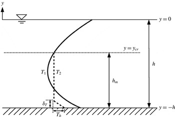
is the average temperature increase over the depth, i.e. the mean temperature increases steadily with time. After the onset of instability, the flow becomes unsteady and exhibits bursts of buoyant plumes from the bottom boundary layer, which then drives vigorous mixing of fluid. Laminar plume behaviour in a quiescent environment with a stable thermal stratification has been studied in Morton (Reference Morton1967) and Wirtz & Chiu (Reference Wirtz and Chiu1974), and it was shown that the plume rise height is determined by the gradient of the background thermal stratification. In figure 1, typical vertical temperature distributions before and after the onset of instability in relatively deep waters with a substantial surface stable stratification are shown. The thickness of the bottom thermal boundary layer reduces after the onset of instability due to a substantial amount of heated fluid being removed from the boundary layer in the form of rising plumes and also due to the induced advection flow limiting the diffusive growth of the thermal boundary layer. Also associated with the plume motion, the water temperature tends to homogenise over the plume rise height. Further, the surface stable layer is not affected by the boundary layer instability and remains stratified, due to the plume penetration being limited to the lower part of the fluid layer.
Schematic showing the bottom thermal boundary layer and the lower mixed layer thickness (
 $h_{m}$
) with typical temperature distributions before (
 $T_{1}$
) and after (
 $T_{2}$
) the onset of instability in relatively deep waters.

The plume penetration is expected to be determined by the location of the point of neutral buoyancy. In the following, a theoretical model for the plume penetration height, i.e. the lower mixed layer thickness (
 $h_{m}$
), is established. As mentioned above, the temperature stratification is destroyed by the plume motion, and hence the temperature distribution tends to homogenise over the lower mixed layer thickness with the vertical temperature gradient significantly reduced over this region. Further, the thickness of the unstably stratified bottom boundary layer is insignificant compared to the total lower mixed layer thickness. The temperature distribution over the lower mixed layer thickness is therefore assumed to be uniform in the following analysis. This assumption is validated via numerical simulation of the flow in the following section along with the proposed theoretical model. The level of neutral buoyancy is denoted by
 $y_{cr}$
. From (3.1), the total temperature increase over the depth is
 $\int _{-h}^{0}T\text{d}y=t$
. From (2.2), in the stable surface layer (
 $y_{cr}\leqslant y\leqslant 0$
) where the flow is approximately quiescent and the vertical length scale is large (
 ${\sim}{\it\eta}^{-1}$
), the following relation holds:
 $$\begin{eqnarray}\frac{\partial T}{\partial t}\approx \exp (y),\end{eqnarray}$$
therefore,
 $$\begin{eqnarray}T\approx t\exp (y).\end{eqnarray}$$
The total temperature increase in this region is:
 $$\begin{eqnarray}\int _{y_{cr}}^{0}T\text{d}y\approx t-t\exp (y_{cr}).\end{eqnarray}$$
Therefore the spatially averaged temperature increase over the region
 $-h\leqslant y\leqslant y_{cr}$
with the length
 $h_{m}$
is:
 $$\begin{eqnarray}\frac{\displaystyle \int _{-h}^{0}T\text{d}y-\int _{y_{cr}}^{0}T\text{d}y}{h_{m}}\approx \frac{t\exp (y_{cr})}{h_{m}}.\end{eqnarray}$$
Further, the local temperature increase at
 $y=y_{cr}$
is obtained from (3.3) as:
 $$\begin{eqnarray}T\approx t\exp (y_{cr}),\end{eqnarray}$$
which is equal to the right-hand side of (3.5); therefore:
 $$\begin{eqnarray}h_{m}\approx 1.\end{eqnarray}$$
This suggests that for
 $h>1$
, the plume penetration is limited and the dimensional lower mixed layer thickness (
 $h_{m}^{\ast }$
) is equal to the attenuation length of the radiation (
 ${\it\eta}^{-1}$
). Even when
 $y_{cr}\rightarrow 0$
, (3.7) holds, and this means that for
 $h<1$
the location of neutral buoyancy does not exist and therefore plumes penetrate the full depth. Numerical validation of the above prediction is discussed in § 4.
3.2. Quasi-steady boundary layer
The boundary layer behaviour after the onset of instability is partly governed by Howard’s theory of intermittent convection in deep layers (Howard Reference Howard1966), which states that an unsteady thermal boundary layer undergoes a cyclic process consisting of the diffusive growth of the thermal boundary layer, the onset of instability when the local Rayleigh number exceeds a critical value, the destruction of the boundary layer in the form of rising plumes and the restoration of the boundary layer by diffusion. Howard’s theory assumes that the fluid layer is infinitely deep and the heat transfer is purely one-dimensional. However, in the present problem with a bounded fluid layer, plumes drive a large-scale circulating flow (bulk flow), which substantially affects the boundary layer stability; it acts to stabilise the unstably stratified thermal boundary layer. The stabilisation of the boundary layer due to the plume-driven circulating flow is illustrated by numerical simulations in the following section. This may also be expected from the linear stability analysis for the Rayleigh–Bénard–Poiseuille flow (Nicolas, Luijkx & Platten Reference Nicolas, Luijkx and Platten2000), which is of a different flow configuration; however, some analogy may apply. Due to the presence of the bulk flow, Howard’s model does not directly apply to the present problem; however, the boundary layer exhibits a cyclic behaviour at the quasi-steady state although the fluctuation is not single periodic as for Howard’s model described above. Therefore, it is appropriate to consider the time-averaged flow field at the quasi-steady state. In what follows, the scaling relations for the time-averaged boundary layer thickness
 ${\it\delta}_{T}$
and perturbation temperature difference across the boundary layer
 $T_{b}$
(refer to figure 1) at the quasi-steady state are obtained.
Following the above discussion and assuming that
 ${\it\delta}_{T}\ll h_{m}$
so that the thermal boundary layer is not affected by the surface layer and the surface boundary, the following balances are obtained for the time-averaged, quasi-steady bottom boundary layer:
 $$\begin{eqnarray}v\frac{\partial T}{\partial y}\sim \frac{\partial ^{2}T}{\partial y^{2}},\end{eqnarray}$$
and
 $$\begin{eqnarray}v\frac{\partial v}{\partial y}\sim \mathit{Ra}\mathit{Pr}T.\end{eqnarray}$$
It follows that:
 $$\begin{eqnarray}v_{p}\frac{T_{b}}{{\it\delta}_{T}}\sim \frac{T_{b}}{{\it\delta}_{T}^{2}},\end{eqnarray}$$
and
 $$\begin{eqnarray}\frac{v_{p}^{2}}{{\it\delta}_{T}}\sim \mathit{Ra}\mathit{Pr}T_{b},\end{eqnarray}$$
where
 $v_{p}$
is the characteristic ascending velocity associated with the plume formation. Further, from the bottom thermal boundary condition (2.4):
 $$\begin{eqnarray}T_{b}\sim \exp (-h){\it\delta}_{T}.\end{eqnarray}$$
Eliminating
 $v_{p}$
from (3.10) and (3.11) leads to:
 $$\begin{eqnarray}{\it\delta}_{T}\sim \left(\frac{\exp (h)}{\mathit{Ra}\mathit{Pr}}\right)^{1/4},\end{eqnarray}$$
and
 $$\begin{eqnarray}T_{b}\sim \frac{1}{\left(\mathit{Ra}\mathit{Pr}\exp (3h)\right)^{1/4}}.\end{eqnarray}$$
The configuration of the flow under consideration is apparently different from the classical Rayleigh–Bénard convection. The classical Rayleigh–Bénard convection is bounded by rigid and fixed-temperature walls, whilst the flow considered here is bounded by a rigid and fixed-heat-flux bottom and a stress-free and adiabatic top, and is subject to a non-uniform volumetric heating associated with the direct absorption of incoming radiation. However, the analogy with the classical Rayleigh–Bénard theory may be applied to derive the scaling relations for
 ${\it\delta}_{T}$
and
 $T_{b}$
as follows. Figure 1 suggests that
 $h_{m}$
may be treated as the size of the convection cell and
 $T_{b}$
as the temperature difference across the convection cell. Consequently, the equivalent Rayleigh number for the analogous classical Rayleigh–Bénard convection is written as:
 $$\begin{eqnarray}\mathit{Ra}_{RB}\equiv \frac{g{\it\beta}T_{b}^{\ast }h_{m}^{\ast 3}}{{\it\nu}{\it\kappa}}.\end{eqnarray}$$
It is noted that
 $h_{m}^{\ast }$
and
 $T_{b}^{\ast }$
in the above equation are dimensional quantities, given as
 $h_{m}^{\ast }=h_{m}/{\it\eta}$
and
 $T_{b}^{\ast }=T_{b}I_{0}/{\it\rho}_{0}C_{p}{\it\kappa}{\it\eta}$
respectively. The classical
 $1/3$
scaling law for the Nusselt number
 $\mathit{Nu}$
is then written as (Priestley Reference Priestley1954; Malkus Reference Malkus1954):
 $$\begin{eqnarray}\mathit{Nu}\equiv \frac{h_{m}\displaystyle \frac{\partial T}{\partial y}\bigg|_{y=-h}}{T_{b}}\sim \mathit{Ra}_{RB}^{1/3}.\end{eqnarray}$$
It is noted (Amati et al.
Reference Amati, Koal, Massaioli, Sreenivasan and Verzicco2005) that the classical scaling law for Rayleigh–Bénard convection is based on the assumption that all the heat transfer occurs within the thermal boundary layers, with the bulk of the fluid layer essentially remaining isothermal and that the two boundary layers behave independently and do not communicate through the bulk flow. The first assumption is shown to be satisfied in the present study, as discussed later. The second assumption is equivalent to the heat flux being independent of the depth of the fluid layer (Castaing et al.
Reference Castaing, Gunaratne, Heslot, Kadanoff, Libchaber, Thomae, Wu, Zaleski and Zanetti1989) and is relevant to
 ${\it\delta}_{T}\ll h_{m}$
in the present flow configuration so that the bottom thermal boundary layer behaves independently of the surface layer and the surface boundary. Solving (3.16) for
 $T_{b}$
yields:
 $$\begin{eqnarray}T_{b}\sim \frac{1}{\left(\mathit{Ra}\exp (3h)\right)^{1/4}},\end{eqnarray}$$
which is identical to (3.14) (except for the
 $\mathit{Pr}$
dependence). Then
 ${\it\delta}_{T}$
is obtained as follows:
 $$\begin{eqnarray}{\it\delta}_{T}\equiv \frac{T_{b}}{\displaystyle \frac{\partial T}{\partial y}\bigg|_{y=-h}}\sim \left(\frac{\exp (h)}{\mathit{Ra}}\right)^{1/4},\end{eqnarray}$$
which is identical to (3.13) (except for the
 $\mathit{Pr}$
dependence). The
 $\mathit{Pr}$
dependence is not determined from the classical Rayleigh–Bénard theory; however, it is not relevant in the present study which focuses on water with a fixed
 $\mathit{Pr}$
as the working fluid. Further, substituting for
 $h_{m}^{\ast }$
and
 $T_{b}^{\ast }$
in (3.15) using (3.7) and (3.17) yields a scaling relation between the equivalent Rayleigh number for the classical Rayleigh–Bénard convection and the flux Rayleigh number used in the present study:
 $$\begin{eqnarray}\mathit{Ra}_{RB}\sim \mathit{Ra}^{3/4}\exp \left(-\frac{3h}{4}\right).\end{eqnarray}$$
The above correlation suggests that the equivalent Rayleigh number for classical Rayleigh–Bénard convection is approximately 2 orders of magnitude smaller than the flux Rayleigh number considered. Amati et al. (Reference Amati, Koal, Massaioli, Sreenivasan and Verzicco2005) found the convergence of
 $\mathit{Nu}$
towards the
 $1/3$
scaling for
 $\mathit{Ra}_{RB}>10^{10}$
. In the following numerical investigation, consistency with the classical scaling is found for the flux Rayleigh number,
 $\mathit{Ra}\gtrsim 10^{8}$
, which is equivalent to
 $\mathit{Ra}_{RB}\gtrsim 10^{6}$
. The discrepancy from the published result (Amati et al.
Reference Amati, Koal, Massaioli, Sreenivasan and Verzicco2005) is most likely due to the differences in the boundary conditions imposed at the bounding surfaces. It is noted that Sparrow, Goldstein & Jonsson (Reference Sparrow, Goldstein and Jonsson1964) found a critical Rayleigh number of 320 for the marginal stability for a rigid and fixed-heat-flux bottom and a stress-free and fixed-heat-flux top, and 1708 for rigid and fixed-temperature top and bottom, both with a linear temperature profile across the depth of the fluid layer.
4. Numerical validation
The validation of the above theoretical analysis is conducted via two-dimensional numerical simulation of the flow in a horizontal fluid layer of depth in the range
 $0.5\leqslant h\leqslant 3.0$
subject to constant and uniform radiation at the water surface with the Rayleigh number in the range
 $10^{7}\leqslant \mathit{Ra}\leqslant 10^{10}$
. The adoption of a two-dimensional numerical model for this type of flow has been justified in Lei & Patterson (Reference Lei and Patterson2005). To provide further verification, a limited number of three-dimensional simulations have also been conducted using computational domains with reduced horizontal extents and reduced grid resolutions in the horizontal directions. Comparisons of the two- and three-dimensional simulation results are discussed at the end of the section. The highest
 $\mathit{Ra}$
considered in this study is equivalent to the physical scenario with solar radiation of
 $I_{0}=1000~\text{W m}^{-2}$
and
 ${\it\eta}\sim 10~\text{m}^{-1}$
, a typical attenuation coefficient for inland waters (Kirk Reference Kirk, De Deckker and Williams1986, Reference Kirk1994). The considered range of
 $h$
corresponds to typical water depths used in laboratory-scale experiments of closely related flows (Coates & Patterson Reference Coates and Patterson1993; Lei & Patterson Reference Lei and Patterson2002a
; Bednarz, Lei & Patterson Reference Bednarz, Lei and Patterson2008). The applicability of the subsequent analysis to larger values of
 $h$
relevant to the physical depths of littoral waters is shown later. The numerical simulation uses the SnS code (Norris Reference Norris2000), which is a non-staggered, Cartesian mesh, finite volume code based on a fractional step method (Armfield Reference Armfield1994; Armfield & Street Reference Armfield and Street2002), with the Adams-Bashforth and Crank–Nicolson time discretisation schemes being used for the advection and diffusion terms, respectively. The code is written in double-precision format. The spatial discretisation of the diffusion terms uses second-order central differencing, whilst the spatial discretisation of the advection terms uses second-order central differencing with the ultra (universal limiter for tight resolution and accuracy) flux limiter (Leonard & Mokhtari Reference Leonard and Mokhtari1990). A variable time step size is used to maintain the CFL (Courant–Friedrichs–Lewy) number within the range 0.15–0.3; the time step size is updated every time step based on the CFL number. Further reducing the CFL number range, which in turn reduces the time step size, has a negligible effect on the solution accuracy (not shown for the sake of brevity). The strongly implicit procedure (sip) (Stone Reference Stone1968) is used for solving the momentum and energy equations, while the bi-conjugate gradient stabilised method (bicgstab) (van der Vorst Reference van der Vorst1981) using a sip preconditioner is used for solving the Poisson pressure correction equation, which is formed directly from the Navier–Stokes equations. The convergence criteria ensure that the root-mean-square value of the cell divergence (the net flux into a finite volume cell) is kept below
 $10^{-8}$
at every time step.
The horizontal extent of the computational domain is
 $0\leqslant x\leqslant 10$
, and the vertical extent is
 $-h\leqslant y\leqslant 0$
with
 $h$
varied over the range
 $0.5\leqslant h\leqslant 3.0$
, the range used in the laboratory experiments, as noted above. The boundary conditions imposed at the horizontal boundaries (
 $y=-h$
and
 $y=0$
) are as aforementioned, whereas the periodic condition with
 $f_{x=0}\equiv f_{x=10}$
, where
 $f$
represents any flow quantity and its derivatives, is applied at the vertical boundaries.
 $2000$
grid points are uniformly distributed in the horizontal (
 $x$
) direction. In the vertical (
 $y$
) direction, the grid size near the horizontal boundaries is
 $4\times 10^{-4}<{\rm\Delta}y<5\times 10^{-4}$
with 1–3 % linear stretching applied, giving at least
 $20$
grid points within the bottom boundary layer after the flow becomes quasi-steady for
 $\mathit{Ra}\leqslant 10^{10}$
; the largest grid size of
 $8\times 10^{-3}<{\rm\Delta}y<1\times 10^{-2}$
is in the centre of the domain; and the total grid points is
 $200$
,
 $360$
,
 $540$
,
 $700$
and
 $900$
for
 $h=0.5$
,
 $1.0$
,
 $1.5$
,
 $2.0$
and
 $3.0$
, respectively. Further increasing the number of grid points has only marginal effect on the solution accuracy, as shown below.
The grid dependence test conducted for the cases of
 $h=0.5$
with
 $\mathit{Ra}=10^{9}$
and
 $\mathit{Ra}=10^{10}$
: (a) the perturbation temperature at the middle of the bottom boundary,
 $(x,y)=(5.0,-0.5)$
and (b) the standard deviation of the temperature over the bottom boundary. The different flow regimes are marked for the case of
 $\mathit{Ra}=10^{9}$
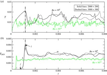
as: (i) the diffusive growth of the boundary layer, (j) the onset of instability, (k) the exponential growth of the perturbation following linear theory, (l) plume formation, and (m) quasi-steady state.

Instantaneous perturbation temperature fields obtained for
 $\mathit{Ra}=10^{9}$
and
 $h=0.5$
at (a)
 $t=0.001$
 $(k)$
; (b)
 $t=0.00115$
 $(l)$
; (c)
 $t=0.0015$
 $(l)\rightarrow (m)$
; (d)
 $t=0.004$
 $(m)$
; and (e)
 $t=0.014$
 $(m)$
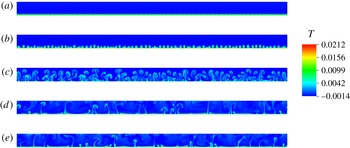
.

Figure 2 shows the results of the grid dependence test for the cases of
 $h=0.5$
with
 $\mathit{Ra}=10^{9}$
and
 $\mathit{Ra}=10^{10}$
, using two different mesh resolutions,
 $2000\times 200$
and
 $3000\times 300$
. Figure 2(a) shows the time series of the perturbation temperature at the middle of the bottom boundary,
 $(x,y)=(5.0,-0.5)$
, and figure 2(b) shows the time series of the standard deviation of the temperature over the bottom boundary. The different flow regimes are marked as (i–m) for the case of
 $\mathit{Ra}=10^{9}$
and
 $h=0.5$
, and the instantaneous perturbation temperature fields corresponding to the flow regimes (k–m) (obtained on the
 $2000\times 200$
grid) are shown in figure 3. The flow regime before the initial peak shown in figure 2(a,b) corresponds to the development of thermal structures in a quiescent environment, which consists of the steady diffusive growth of the bottom boundary layer (i), the onset of instability (j) and the exponential growth of the perturbation following the linear theory (k) (figure 3(a)). The sudden reduction after the peak is due to the primary plume formation (l) (figure 3
b), which destroys the boundary layer and drives a circulating flow (figure 3
c), leading to a sudden reduction in the boundary layer temperature (figure 2
a). The circulating flow acts to stabilise the bottom boundary layer, as discussed earlier; therefore the signal reaches a plateau (m) after the reduction, i.e. quasi-steady state (figure 3
d,e). It is shown that the variation between the results obtained with two different mesh resolutions is only marginal in both cases, and the grid dependence is even weaker for all other cases with reduced
 $\mathit{Ra}$
and increased
 $h$
, i.e. reduced bottom heating. Therefore, the coarser grid is used, to minimise computational requirements. Time-averaged quantities are calculated in the quasi-steady flow regime over time periods of
 $t\approx 0.21$
for the
 $\mathit{Ra}=10^{7}$
flows;
 $t\approx 0.072$
for the
 $\mathit{Ra}=10^{8}$
flows;
 $t\approx 0.014$
for the
 $\mathit{Ra}=10^{9}$
flows; and
 $t\approx 0.007$
for the
 $\mathit{Ra}=10^{10}$
flows.
Instantaneous perturbation temperature in the steady flow regime (
 $t=0.00143$
) and time-averaged perturbation temperature in the quasi-steady flow regime plotted over the depth for
 $\mathit{Ra}=10^{9}$
and
 $h=2.0$
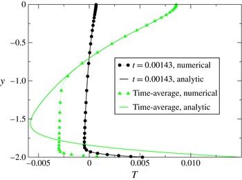
, compared with the analytic solution (3.1).

In figure 4, instantaneous perturbation temperature at
 $t=0.00143$
and time-averaged perturbation temperature over
 $0.0144\leqslant t\leqslant 0.0286$
in the quasi-steady flow regime, spatially averaged over
 $0\leqslant x\leqslant 10$
, are plotted over the depth for the case of
 $\mathit{Ra}=10^{9}$
and
 $h=2.0$
. In the figure, the corresponding analytic solutions from (3.1) are also shown for comparison. At
 $t=0.00143$
, the flow is steady, hence the numerical and analytic solutions perfectly agree with each other, as expected. The time-averaged profile obtained in the quasi-steady flow regime perfectly agrees with the corresponding time-averaged analytic solution in the surface stable layer. This confirms that the surface layer is not affected by the bottom boundary layer instability and the consequent plume activities. Further, it is shown that the quasi-steady time-averaged bottom boundary layer is substantially thinner than the corresponding analytic solution, which is evidently a consequence of the plume formation as discussed earlier. It is also shown that the temperature distribution over the central region (above the thin bottom boundary layer and below the surface layer) is approximately uniform. This verifies the assumption for the theoretical analysis in § 3.1 and satisfies one of the assumptions for the classical
 $1/3$
scaling discussed in § 3.2. Consistent flow characteristics have also been confirmed for other values of
 $\mathit{Ra}$
and
 $h$
over the ranges
 $10^{7}\leqslant \mathit{Ra}\leqslant 10^{10}$
and
 $0.5\leqslant h\leqslant 3.0$
respectively.
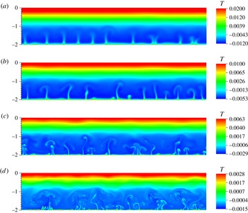
In figure 5, instantaneous perturbation temperature fields obtained in the quasi-steady flow regime for the different values of
 $\mathit{Ra}$
and
 $h=2.0$
are shown. Clearly, the plume penetration is limited to the lower part of the flow domain, and the upper part remains stratified. It is seen that the plume penetration height (i.e. lower mixed layer thickness,
 $h_{m}$
) is approximately constant for the different values of
 $\mathit{Ra}$
and
 $h_{m}\approx 1$
. Similar observations have been made for other values of
 $h$
for
 $h>1$
. Further, it is clear that the bottom boundary layer thickness reduces, and the flow exhibits an increasingly chaotic behaviour with increased small-scale structures as
 $\mathit{Ra}$
increases.
Instantaneous perturbation temperature fields obtained in the quasi-steady flow regime for
 $h=2.0$
and (a)
 $\mathit{Ra}=10^{7}$
(at
 $t=0.073$
); (b)
 $\mathit{Ra}=10^{8}$
(at
 $t=0.03$
); (c)
 $\mathit{Ra}=10^{9}$
(at
 $t=0.016$
); and (d)
 $\mathit{Ra}=10^{10}$
(at
 $t=0.007$
).

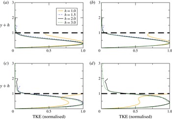
In figure 6, the distribution of turbulence kinetic energy (
 $\text{TKE}=\overline{u_{i}^{\prime }u_{i}^{\prime }}/2$
, where
 $u_{i}^{\prime }$
is the velocity fluctuation and the overbar is the time-averaging operator) over the depth, spatially averaged over
 $0\leqslant x\leqslant 10$
, is shown for different cases (
 $h\geqslant 1$
). In the figure, the ordinate has been translated by
 $h$
to fix the location of the bottom boundary for different cases. It is shown that TKE undergoes a sudden reduction in the vicinity of
 $h_{m}\approx 1$
in the cases with
 $h>1$
and remains small above this location, suggesting that the flow is substantially stabilised above this location and mixing takes place only over a limited distance from the bottom, consistent with the results shown in figure 5. This is not the case for
 $h\leqslant 1$
where mixing takes place over the full depth. The above results are in excellent agreement with the theoretical model (3.7); therefore it is confirmed that
 $h_{m}^{\ast }\approx {\it\eta}^{-1}$
for
 $h>1$
, which applies to the physical scenario in littoral waters.
The distribution of TKE over
 $y+h$
for (a)
 $\mathit{Ra}=10^{7}$
; (b)
 $\mathit{Ra}=10^{8}$
; (c)
 $\mathit{Ra}=10^{9}$
; and (d)
 $\mathit{Ra}=10^{10}$
. TKE has been normalised by the maximum value over the depth.

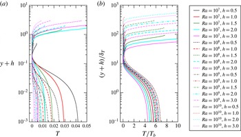
Figure 7(a) shows the time-averaged perturbation temperature profile over the depth, spatially averaged over
 $0\leqslant x\leqslant 10$
, for different cases. Again, the ordinate has been translated by
 $h$
to fix the location of the bottom boundary for different cases, and the abscissa has also been translated to fix the minimum temperature at
 $T=0$
. In order to validate the scaling relations for the time-averaged boundary layer thickness
 ${\it\delta}_{T}$
(3.13) and perturbation temperature difference across the boundary layer
 $T_{b}$
(3.14), the ordinate of figure 7(a) is normalised by the scaling for
 ${\it\delta}_{T}$
and the abscissa is normalised by the scaling for
 $T_{b}$
. The normalised profiles are then plotted in figure 7(b). The approximate collapse of the normalised profiles in the bottom boundary layer region shown for
 $\mathit{Ra}\gtrsim 10^{8}$
confirms the validity of the scalings and consistency with the classical scaling (3.16), whilst the increased scattering for the
 $\mathit{Ra}=10^{7}$
cases indicates the deviation from the classical scaling and is evidently associated with the increased
 ${\it\delta}_{T}$
with reducing
 $\mathit{Ra}$
, therefore failing to satisfy the underlying assumption,
 ${\it\delta}_{T}\ll h_{m}$
.

As noted earlier, three-dimensional numerical simulations have been conducted for the lowest and highest
 $\mathit{Ra}$
cases with the smallest and largest values of
 $h$
respectively, i.e.
 $\mathit{Ra}=10^{7}$
cases with
 $h=0.5$
and
 $3.0$
and
 $\mathit{Ra}=10^{10}$
cases with
 $h=0.5$
and
 $3.0$
. Due to the associated substantial computational costs, the three-dimensional simulations use computational domains with reduced horizontal extents (
 $0\leqslant x\leqslant 1$
and
 $0\leqslant z\leqslant 1$
), and the grid spacing in the horizontal directions is made twice as large as that of the two-dimensional simulations described above, i.e. a uniformly distributed mesh with
 $100$
grid points in each of the two horizontal directions, whilst in the vertical direction the same grid resolution as the above-described two-dimensional simulations is adopted for a given
 $h$
. The boundary conditions imposed on the horizontal and vertical boundaries are as described earlier for the two-dimensional simulations. Additional two-dimensional simulations with the same horizontal extent (
 $0\leqslant x\leqslant 1$
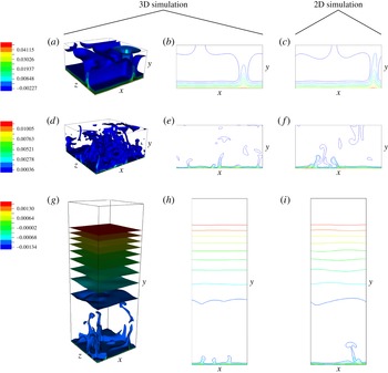
) and grid resolution as those of the three-dimensional simulations have also been conducted. Figure 8 shows instantaneous perturbation temperature fields in the quasi-steady flow regime obtained from two- and three-dimensional simulations with reduced horizontal extents and reduced horizontal grid resolutions for the
 $\mathit{Ra}=10^{7}$
case with
 $h=0.5$
and the
 $\mathit{Ra}=10^{10}$
cases with
 $h=0.5$
and
 $3.0$
. In each case, the two- and three-dimensional simulation results show similar flow behaviours, especially in the small
 $\mathit{Ra}$
case.
Instantaneous perturbation temperature fields obtained from two- and three-dimensional simulations with reduced horizontal extents and reduced horizontal grid resolutions for: (a–c)
 $\mathit{Ra}=10^{7}$
and
 $h=0.5$
(
 $t=0.21$
); (d–f)
 $\mathit{Ra}=10^{10}$
and
 $h=0.5$
(
 $t=0.006$
); and (g–i)
 $\mathit{Ra}=10^{10}$
and
 $h=3.0$
(
 $t=0.006$
). (a,b,d,e,g,h) Three-dimensional (3D) simulation results and (c,f,i) two-dimensional (2D) simulation results. (b,e,h) Sliced views of (a,d,g) at the
 $z=0.5$
plane respectively.

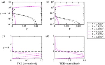
In figure 9, the two- and three-dimensional simulation results for the time-averaged perturbation temperature profile over the depth (as shown in figure 7
a) and for the normalised TKE (as shown in figure 6) for
 $h=3.0$
are compared. The variations in the time-averaged perturbation temperature profiles obtained from the original two-dimensional simulations and the two- and three-dimensional simulations using reduced horizontal extents and reduced grid resolutions are found to be only marginal. Further, the results for the TKE distribution obtained from the two- and three-dimensional simulations with reduced horizontal extents and reduced horizontal grid resolutions are both consistent with the results of the original two-dimensional simulations, showing a sudden reduction in the vicinity of
 $h_{m}\approx 1$
. This provides further verification for the theoretical model (3.7). Overall, the adoption of a two-dimensional numerical model is verified without adversely affecting the results reported in this study.
Comparison of two- and three-dimensional simulation results, referred to as 2D and 3D, respectively. (The superscript
 $\ast$
represents the simulations with reduced horizontal extents and reduced horizontal grid resolutions, as described in the text.) Time-averaged perturbation temperature profile over
 $y+h$
for (a)
 $\mathit{Ra}=10^{7}$
and (b)
 $\mathit{Ra}=10^{10}$
. The normalised TKE over
 $y+h$
for (c)
 $\mathit{Ra}=10^{7}$
and (d)
 $\mathit{Ra}=10^{10}$
, for
 $h=3.0$
only.

5. Conclusions
The present study has focused on the radiation-induced natural convection in natural water bodies typically with slowly varying topography. In such water bodies, the stability of the bottom thermal boundary layer has important implications for water quality as the thermal instability in the form of rising plumes drives vigorous mixing of the water. In relatively deep waters with a substantial surface stable stratification, the plume penetration is limited and so is the vertical mixing; therefore the lower mixed layer thickness is an important parameter for water quality management. A theoretical model for the lower mixed layer thickness has been developed in the present study (§ 3.1) and excellent agreement with numerical simulations has been demonstrated (figures 5 and 6). It was concluded that the dimensional lower mixed layer thickness (
 $h_{m}^{\ast }$
) is equal to the attenuation length of the radiation (
 ${\it\eta}^{-1}$
), which has important implications for the transport of pollutants and nutrients in the water body. Further, scaling relations for the quasi-steady boundary layer have been obtained via two separate approaches (§ 3.2) and the validity of the scaling relations has been confirmed for
 $\mathit{Ra}\gtrsim 10^{8}$
by numerical simulations (figure 7).
Acknowledgements
This research was financially supported by the Australian Research Council (DP120104849) and The University of Sydney. The authors wish to thank the anonymous reviewers for very useful comments, which helped to improve the quality of the paper significantly.