Model Description

Sea ice is considered a two-dimensional (2-D) continuum described by the standard prognostic variables ice thickness (h), areal coverage or ice concentration (A), and horizontal ice velocity (u). The spatial and temporal evolution of ice cover is determined from extended-continuity equations, including thermodynamic source and sink terms for h and A. Equations for u are derived from a momentum balance including wind stress, water stress, Coriolis force, sea-surface tilt, and internal forces due to ice deformation. A viscous-plastic rheology following Reference HiblerHibler (1979) describes the internal forces. Thermodynamic growth and melting of sea ice is derived from the energy balance outlined by Reference Parkinson and WashingtonParkinson and Washington (1979). The main differences from the Reference HiblerHibler (1979) model are (1) a numerical upstream scheme for advection, avoiding negative ice thicknesses, (2) no explicit diffusion in the continuity equations, (3) optimized drag coefficients (Reference HarderHarder, 1994; Reference FischerFischer, 1995), and (4) inclusion of a prognostic snow layer (Reference Owens and LemkeOwens and Lemke, 1990).

The physical equations are implemented as a numerical model running on a rotated spherical grid covering the whole Arctic, with a spatial resolution of 1° and a daily time-step. Daily surface atmospheric-forcing data for wind, air temperature, and humidity are taken from European Centre for Medium-Rauge Weather Forecasts (ECMWF) analyses for 1986–92. Cloudiness and precipitation, are prescribed as climatological means. Ocean currents are taken from a separate ocean model (Reference Gerdes and KöberleGerdes and Köberle, 1995).

Roughness (R) and age (a) of sea ice are introduced as scalar variables, with their spatial and temporal evolutions described by two additional, prognostic budget equations:

where the lelthand side describes the local rates of change and advection, and the righthand side describes the source and sink terms for the roughness and the age of sea ice.

R (Reference HarderHarder, 1996) is defined as the accumulation of deformation of sea-ice cover by internal forces, given as an energy per area in J m⁻². These internal forces, acting as a source of ice roughness, are derived as the product of the stress tensor (σ) and the strain rate from the viscous-plastic rhcology by standard continuum mechanics (Reference RothrockRothrock, 1975). Newly frozen ice is considered to have no original roughness. As the ice volume is regarded as a carrier of ice roughness, it is assumed that R vanishes at the same rate as the ice-volume melts. (A more elaborate approach might take into account that ridges tend to melt faster than level ice.)

The age (a) of sea ice is defined as a scalar quantity with the dimension of time. At the point when sea water freezes to sea ice, its age is defined as zero. Then, the ice grows older by a rate of one, so time is the source of age. Further freezing adds young ice to already-existing older ice. When new ice is frozen, a new, reduced age is determined as a volume-weighted average of all ice in a model gridcell. Freczing of new ice is the sink of a. Similarly, a volume-weighted mean a is calculated after each time-step, when advection has mixed sea ice of different regions and different ages. When all these terms describing the age of sea ice are added together, the prognostic equation (Equation (2)) is obtained. A more detailed description of the simulated age of sea ice, applied to a Weddell Sea ice model, is given by Reference Harder, Lemke, Johannessen, Mueneh and OverlandHarder and Lemke (1994).

The prognostic equations (Equations (1) and (2)) appear similar to a prognostic equation describing the evolution of ice thickness. But, it must be noted that the source terms on the righthand side of the equation are different. The source of R is caused by internal forces resulting from sea-ice dynamics, thus R represents the integrated history of the deformation of ice volume. Ice that is grown purely thermo-dynamically may reach considerable thickness, but has no roughness, whereas even thin ice quickly becomes rough in areas with high deformation. Roughness and ice thickness are physically different quantities, with roughness characterizing the contribution of deformation to ice-thickness buildup.

The age of sea ice is a physical quantity that is different from ice thickness and roughness. Age measures the time required to build up an ice cover of actual thickness and roughness. Generally, older ice tends to be thicker and rougher than young ice, as it has had more time to grow and to undergo deformation. But, this depends on the geographical region and the season, so thickness, roughness and age describe different aspects of the development of the sea-ice cover.

Other attempts (e.g. Reference Flato and HiblerFlato and Hibler, 1991; Reference HarderHarder and Lemke, 1994; Reference Kwok, Rothrock, Stern and CunninghamKwok and others, 1995) have been made to characterize roughness or age of sea ice by introducing different ice classes. These more sophisticated multi-level models describe certain properties of sea ice that cannot be accounted for in the descriptions of roughness and age discussed above. However, these multi-level models depend on a number of empirical or arbitrary parameterization, although the one-class approach is easy to implement in existing large-scale sea-ice or climate models, with the cost of additional computing being small.

In the model, Lagrangian trajectories are obtained from an interpolation of the simulated Eulerian v elocities to subgrid scales. The simulated trajectories start at the same date and position as observed buoys. Then, in each time-step, the model calculates the motion of a hypothetical ice particle from its latest simulated position to a new position, according to the ice velocity prognosed for the actual time-step and area. The simulated trajectory then comprises a set of simulated positions reached successively by the hypothetical ice particle. This simulated trajectory is similar to the paths of observed buoys that report their successive positions as a function of time. Details of the numerical procedure are described by Reference HarderHarder (1994).

It is important to note the difference between the simulated trajectories described here and the progressive vector plots used in most previous investigations of sea-ice motion (e.g. Reference Hibler and ArkleyHiblerand Ackley, 1983; Reference Ip, Hibler and FlatoIp and others, 1991; Reference Vihma and LauniainenVihma and Launiainen, 1993; Reference Flato and HiblerFlato and Hibler. 1995). Progressive vector plots take the position of an observed buoy to calculate the simulated velocity at this given point. In the next time-step (and all succeeding ones), the observed position is used for the intercomparison of model and buoy velocities. The progressive vector plot scheme compares model velocities with buoy data along a prescribed path taken from observations, instead of predicting a trajectory independent of observations.

Naturally, simulated trajectories are much more sensitive to errors in forcing data or in the physical model: errors occurring when a simulated trajectory is being calculated will accumulate and disturb the prognoses in succeeding time-steps, making the simulated trajectory very sensitive to changes in forcing and physical parameterizations.

This high sensitivity of simulated trajectories qualifies them as valuable tools for model verification. While differences between different ice-dynamics models often appear small when measured by progressive vector plots or monthly mean motion fields, the differences become more visible when the models simulate trajectories. Thus, the simulation of trajectories is one of the most rigorous tests of sea-ice dynamics.

Simulation Results and Comparison with Observations

Figure 1 shows the simulated sea-ice roughness for February 1990. The greatest amount of roughness is found north of Greenland and the Canadian Archipelago, whereas the least amount occurs north of Siberia over the Eurasian Shelf. Moderate, but still recognizable, roughness prevails in the central Arctic. As a result of the advection in the Beaufort Gyre, a tongue of rough ice extends westward from the Canadian Archipelago towards the Bering Strait. A similar spatial pattern, but one varying in detail due to the changes in the daily wind field, is found when sea-ice roughness for other months is simulated.

Fig. 1.

Simulated sea-ice roughness (10⁶ Jm⁻²) in February 1990.

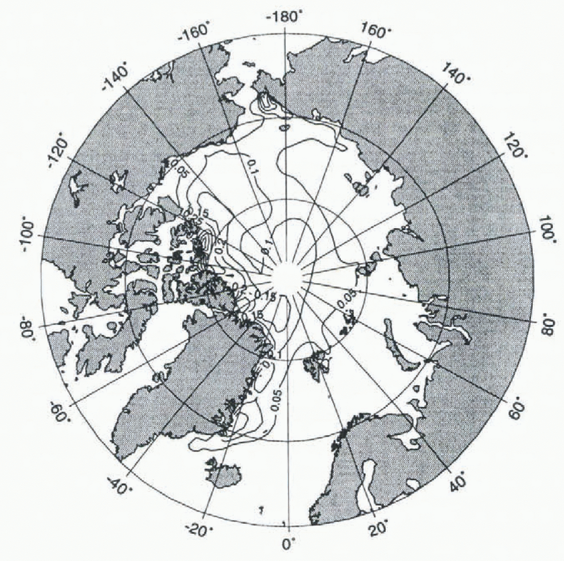
Observations of sea-ice roughness are available from submarine-borne upward-looking sonars, at least for the western Arctic (Reference Bourke and McLarenBourke and McLaren. 1992). Expeditions and Russian data covering the eastern Arctic generally show lower values of ice roughness than those observed north of the American continent. In qualitative comparison, the simulated roughness pattern agrees well with the fact that thick, deformed multi-year ice is observed north of Greenland, whereas thinner, smoother first-year ice occurs over the Eurasian Shelf.

Observations from upward-looking sonars usually describe sea-ice roughness by the geometrical properties of the ice surface (e.g. as mean ridge-keel frequency or keel depth along a cruise track (Reference Bourke and McLarenBourke and McLaren, 1992)). This geometrical roughness is not the same physical quantity as the roughness R, which is energetically defined. However, the different definitions of roughness, depending on the method of measurement or simulation, are related: rough ice, with keels pressed deep into the water and sails exiending well above sea level, contains a significantly higher amount of potential energy than level ice. Energy input from external forcing, such as strong winds or ocean currents, is required to build up rough, deformed ice. Only a part of this energy supply increases the potential energy stored in deformed ice. whereas other fractions are used to break up the ice, or are dissipated in frictional losses. Numerical at simulations of the small-scale process of ridging estimate that about 20% (Reference Hopkins, Hibler and FlatoHopkins and others, 1991) of total ridging work increases the potential energy of the ice cover. More recently, improved simulations have produced a smaller range (5-10%) of values (Reference Flato and HiblerFlato and Hibler, 1995).

The potential energy stored in deformed ice can thus be derived from the observed geometrical properties of the sea-ice surface, such as keel depth and sail height, spatial frequency, probability function, etc. Steiner personal communication from N. Steiner, 1996) gives a preliminary estimate of about 5-10kJ m⁻² of mean potential energy per area stored in pressure ridges as a typical value for the central Arctic. The large-scale model predicts typical values of the roughness (R), representing the accumulated total ridging work per area, in the range of 50-150 kJ m⁻² in the central Arctic. Between 3 and 20% of the total work is available to increase potential energy. This ratio fits well with the results of the small-scale simulations (Reference Hopkins, Hibler and FlatoHopkins and others, 1991; Reference Flato and HiblerFlato and Hibler, 1995) described above.

These figures show how different definitions of roughness, based on energy calculations (total ridging work) or geometrical properties (potential energy), can be finked. Although the task of establishing a sound relation between different roughness definitions is still in progress, these preliminary results indicate a promising fit of model prognoses with observed sea-ice roughness.

The simulated age of sea ice, given in days, is shown in Figure 2 for February 1990. The pattern looks similar to, but not exactly the same as, the roughness pattern. Youngest ice of only 50–100 days is simulated for the Eurasian Shelf region, while the oldest ice (<1000 days: is found north of Greenland. A tongue of old ice advected in the Beaufort Gyre is clearly visible north of Canada. It must be borne in mind that simulated age is a mean value, vertically averaged over all ice layers, and also spatially averaged over the area (110 × 110 km² of each gridcell. Thus, there are individual ice floes that are older or younger than the large-scale mean age of sea ice given in Figure 2.

Fig. 2.

Simulated age of sea ice (days) in February 1990.

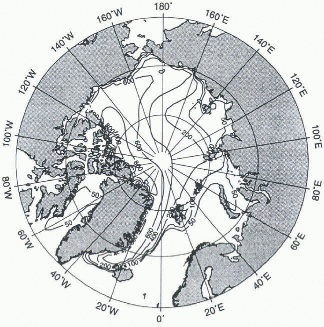
Observations of multi-year ice concentrations are available from satellite-borne observations (SMMR, SSM/I) measured at different microwave frequencies (Reference Gloersen, Campbell, Cavalieri, Comiso, Parkinson and ZwallyGloersen and others, 1992). These observations show high multi-year concentrations north of Greenland and Canada, whereas mostly first-year ice is observed over the Eurasian Shelf. In the central Arctic, a mixture of first-year and multi-year ice dominates. Although the observed multi-year ice concentration does not represent exactly the same physical quantity as the simulated age of sea ice, it is a reasonable and useful observed variable that distinguishes regions of old and new ice. The general spatial pattern of the observed multi-year ice concentration is well reproduced by the simulated age.

However, there remains a discrepancy between the definition of the simulated age (a), defined as a vertical mean through the ice column, and the rather crude distinction between first-year and multi-year ice. derived from observations of the ice surface. While the model variable a really integrates the history of the ice volume, satellite observations give only an estimate of the relative fraction of two ice classes, based on measurements of surface properties that also vary with precipitation, air temperature, etc.).

Other models (e.g. Reference Kwok, Rothrock, Stern and CunninghamKwok and others, 1995) attempt to describe the age of ice by distinguishing between the two ice classes, thus giving a description of the sea-ice age that is closer to satellite-observed quantities. However, this advantage should be weighed against the problems that all multi-class models need to address: the definition of ice classes in the first place, description of transition processes, and the separate thermodynamic (and maybe dynamic) evolution of each class.

Simulated trajectories of sea ice, compared with observed buoy tracks, are shown in Figure 3. The only information from observations passed to the model are the starting position of the buoys and the date of the trajectories, with the further trajectories fully simulated by the model without reference to observations. The observed trajectories are remarkably well simulated by the model for periods as long as one year. However, it must be noted that the buoy data derive from selected information from >200 datasets available for the simulated period, and that some of the simulated trajectories (not presented) do not fit the data derived from some of the other buoys equally well. This underlines the need for further model improvements, which can now be achieved by comparing simulated and observed trajectories (Reference Drinkwater, Fischer, Kreyscher and HarderDrinkwater and others, 1995). By the definition of a quantitative error function (Reference FischerFischer, 1995) that measures the deviations between simulated and observed buoy tracks, different models can be tested in order to find the optimal one to simulate sea-ice drift.

Fig. 3.

Simulated (thick) and observed (thin) trajectories of sea-ice drift.

Discussion and Conclusions

Roughness, age and Lagrangian trajectories have been introduced as three new sea-ice parameters in a large-scale sea-ice model. The simulation results are generally in agreement with the observations available. Lagrangian trajectories are observed with ice-drift buoys, and multi-year ice concentrations are detected with remote-sensing techniques. Simulated roughness, based on energy calculations, shows a similar spatial pattern as that of observed roughness based on surface geometry. The paper has outlined how geometrical roughness features can be related to the total ridging work predicted by the model, with preliminary results showing a reasonable correlation. A permanent global observation of sea-ice roughness from radar sensors will be available when evaluation algorithms are established. Further investigations are required to determine the relationship between different definitions of roughness in measurements (upward-looking sonars, radar) and models.

This article has shown three examples of how additional variables and methods describing the evolution of sea-iee cover provide for the use of a much broader set of observational data to verify the models. The important task for the future lies in compiling all observations available to a standard verification dataset, and defining a quantitative error function for measuring the deviations between observations and simulations (Reference Kreysehcr, Harder and LemkeKreysehcr and others, 1997). This work is carried out in the framework of the WCRP Sea Ice Model Intercomparison Project (SIMIP) outlined by Reference Lemke, Hibler, Flato, Harder and KreyseherLemke and others (1997).