THE 1940s

Real history does not block itself out by decades, but we can use such rough milestones here. The 1940s saw the first serious scientific use of survey research to examine voting behavior more fully. Under the direction of Paul Lazarsfeld, the Bureau of Applied Social Research at Columbia University interviewed a probability sample of Erie County, Ohio, during the Roosevelt–Wilkie presidential race. The study design was remarkably avant-garde. Citizens initially interviewed in the spring were reinterviewed multiple times as the campaign progressed. Lazarsfeld, a veteran of market research, wanted to watch the candidates try to sell their greater merits to the voters in the same mode that commercial enterprises try to out-advertise their competitors. This “panel” design would chronicle the progressive luring of voters into one camp or the other, once the summer nominating conventions had selected the candidates. A serious problem developed, however, when it was discovered that an embarrassing fraction of Erie County voters already knew which party they would vote for in November even before the candidates were chosen. These spring decisions undercut the clever design, although the final report, The People's Choice (1944), made major contributions by shifting attention to groupings defined by social class, religion or urban-rural residence, which showed distinctive preferences for one party or the other. A second Bureau voting study carried out in Elmira, New York during the 1948 presidential campaign gave more attention to the role of interpersonal influence in primary groups in maintaining these partisan colorations in the larger groupings.

THE 1950s

Lazarsfeld was in effect a social psychologist, but his Bureau was lodged in the Sociology Department, and the focus on primary and secondary groups fit with a traditional sociological perspective on voting. This focus seemed parochial to some. There was also restiveness in the broader academic community at the narrow county venues of the Bureau work, when reliable national samples could now be interviewed instead. (The Bureau had not stayed local by choice: it had no national field staff.) Actually, the National Opinion Research Center (NORC), then at the University of Denver, had done a national voting study in 1944, but no major report was made from it. By 1952, the Survey Research Center at the University of Michigan had won a grant for a large-scale study of the first Eisenhower election. The Principal Investigator, Angus Campbell, was a social psychologist, as was the more junior Gerald Gurin, but the other junior, Warren Miller, had serious political science credentials. Moreover, the grant had been won through the good offices of the new Political Behavior Committee of the Social Science Research Council, where Campbell was a member, and first David Truman of Columbia, and later V.O. Key of Harvard were chairmen, pure political scientists both. So the stage was set for turf wars between the sociological and the political science “perspectives” on voting.

In due time (1959), Key and Frank Munger made the elegant case for the political science perspective, relative to the sociological one: political scientists needed to understand shifts in vote outcomes of 5% and 10% or more in election returns over intervals as brief as two to four years, when large social groupings were changing their size only glacially if at all. But at the time when I joined the Election Study staff in 1956, the debate swirled around relative correlation sizes. On one hand it was pointed out that the partisan coloration of sociological groups was less than overwhelming, showing correlations with vote divisions that were rarely much above r = .30. This was well below the correlations generated between the three motivational “orientations” (party, candidates, and issues, which were the central predictors for the Michigan social psychologists) and the final presidential vote in 1952. Naturally, the sociologists were equally condescending about the Michigan “discovery” that voters who liked a party, its candidates, and its platform were much more likely to vote for it than the competitor. Our correlation between vote intention just before the election and the later reported vote was even higher!

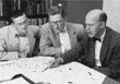
The Making of The American Voter. In June, 1956, Philip E. Converse (above left), Warren E. Miller (above center), and Angus Campbell (above right) were examining maps of the Primary Sampling Units selected for the fall national study of the presidential election, to be later reported as The American Voter. Donald E. Stokes (left) would arrive shortly after, fresh from Yale, to complete the crew. Image #bl005607 of Converse, Miller and Campbell courtesy of Bentley Historical Library, University of Michigan. Photo of Donald Stokes courtesy of Clem Fiori.

I found this discussion embarrassing, although as the most junior member of the 1956 election crew, I felt I should keep my feelings under my hat, given that our side was the big-correlation one. Yet I found myself driven to erect some kind of intellectual structure that to my eye would properly halve the distance in the dispute. I wrote this up as a term paper in my last graduate seminar, unbeknownst to my new colleagues. The Visiting Professor, who presumably knew little about the debate, was so enthusiastic about the paper that he suggested we coauthor it. I instantly said that it was spoken for in my shop, which it was not. But his reception did embolden me to show it to my colleagues, who to my relief reacted with equal enthusiasm. So it became Chapter 2 of The American Voter (Campbell et al. 1960), “funnel of causality” and all.

THE 1960s

This decade opened auspiciously for our Election Study crew. The American Voter (Campbell et al. 1960) was off to the press, and we were descending on new data from our 1958 and 1960 data collections. There were two novelties here: we had converted the 1956 study into a panel, with repeat interviews in 1958 and 1960. More dramatically, Warren Miller (Miller and Stokes 1963) had piggy-backed on the main study an investigation of the role that elections played in the policy representation of the Common Man. This involved interviews with 1958 candidates for Congress running in our primary sampling areas. Data were collected to match the issue content of the voter study, including the candidate's own issue positions and his estimate of the opinion of the constituents on these issues. Finally, roll-call vote data related to these issues cast in the next session of Congress by winners were harvested.

This was a dynamite package of information, and what happened when the complex modules were interlocked and examined remains as one of the most noteworthy beads on the string I am pursuing here. Miller looked first at the correlations between voter issue preferences within each congressional district and the ultimate roll-call votes of their representatives in Congress. It was a disaster. All of these correlations, across various issue domains, were what some wag once called the “Irish correlations”: O'Three, O'Five, O'One. In short, no statistically significant vestige of “representation” could be found at all! A marvelous and costly design had somehow been brought low.

After a period of depression, Miller wisely retraced his steps. He had organized his first runs as bonds between each Represenative and each of his constituents taken separately, such that the N of paired values was the N of all respondents. On review, he realized that it would be no insult to the theory to organize the runs differently, such that each roll-call vote is paired with the mean issue position in that representative's district, with the paired values reduced to the N of representatives. With district opinion aggregated in this way, numerous reassuring relationships winked into view. These correlations were not overwhelming, but they were indeed statistically significant (Miller and Stokes 1963).

Amid this excitement, I was examining the results of our four-year panel, and discovering that in some distressing degree, citizen positions on issues that we considered among the most polarizing of the period were remarkably poorly correlated from one expression to the next by the same respondents. A little reverse engineering suggested that although the fraction varied somewhat from issue to issue, numerous respondents were answering the items so haphazardly from one interview to the next that their “convictions” on these matters seemed little more than Brownian motion. I was writing the “Belief Systems” essay (Converse 1964) at the time, and I was on the brink of writing a final section that would proclaim a sort of simplistic “single-peak” model of the electorate where political issues were concerned, such that the voters nearest the peak in political attentiveness would be largely responsible for the intelligible portion of mass opinion. But I had to stop and test out this growing impression, and soon convinced myself that it was too simple a model by far. This forced me to do an unexpected section entitled “Issue Publics,” because the data were speaking loudly that although there was indeed some upper crust of knowledgeable “generalists,” there were also a lot of foothills populated by ardent specialists on issue domains like gun control or civil rights.

I did one other methodological analysis with the four-year panel which will have echoes later in this piece. By the final wave (postelection, 1960), we were approaching attrition of a quarter of the respondents we had begun with, and it seemed likely that the loss was heaviest among those who knew least about politics and found hour-long interviews on the subject embarrassing. I therefore wanted to know how badly damaged our later results might be, given such significant attrition. This was easily done by contrasting the distributions on variables in the first wave among those who would survive until the panel's end, with those exiting before the end. To my surprise, a review of all of the variables in the first wave showed that differences between the stayers and leavers rarely even approached significance, save at one point. On our main measure of personal political involvement, the stayers were very significantly more involved than the dropouts. If this was so, were there parallel distortions in our other variables correlated with involvement? No, but this was a function of the fact that no other variables in the study were closely correlated with political involvement. Its largest correlation was with education, but this was only about r = .30. To be sure, stayers were more highly educated than leavers in an absolute sense, but still not significantly so.

THE 1970s

By the beginning of the 1970s, I was working primarily in other vineyards than election studies, although I did monitor the area closely for more beads on the string I was following. This decade was noteworthy in part because of the healthy flowering of revisions and updating on the basic notions outlined in The American Voter (Campbell et al. 1960). These took many shapes and forms, but the most persuasive to me, at least, were those documenting the proposition that the 1952–1960 period of our earliest studies was an uncommonly quiet one, soon to be broken by the cresting tumult of both the civil rights movement and the Vietnam War. We were not entirely unaware of this fact even at the time, having labeled it a “steady-state” period where the partisan division of the electorate was concerned, at least relative to the several grand realignments frozen in the long-term U.S. voting record.

Among the revisionist statements, one of the most wide-ranging and well documented was represented by Norman Nie and his collaborators at the University of Chicago. A 1973 article showed that the very weak levels of constraint registered by the policy issues of the 1950s had tightened around the time of the relatively ideological Johnson/Goldwater election of 1964, and had remained high for the period thereafter (Nie and Andersen 1973). These analyses were soon updated and enlarged in The Changing American Voter (Nie, Verba, and Petrocik 1976, 1979). In addition to some strengthening of policy attitudes, these authors showed that there was some weakening of party identifications, in several senses at once. Fewer citizens called themselves “strong” Democrats or Republicans, and the “independents” in the middle became more numerous. Moreover, for any given strength of identification, voters showed an increased likelihood of defecting to the opposing party in their votes. There was also additional evidence that attitudes toward parties as an element on the election scene were growing more negative. Thus the large gap between party and issue motivations so noteworthy in the 1950s had narrowed significantly (although hardly to the point of inverting) by the 1970s.

At least equally notable as an event in this decade had nothing to do with revisionism. This was Gerald Kramer's 1971 study predicting the aggregate vote for Congress, 1896–1964, essentially from four economic variables, with multiple correlations mounting into the .80s, or two-thirds of the temporal variance in the vote accounted for. At first blush it seemed hard to square this work with the sea of noise in voter opinions, including economic ones, found in our studies. But of course it is easy to see that there is no incompatibility here, and for several reasons. One is that most opinion change that is statistically significant at the margin in the short term sweeps over only small percentage ranges, save for such rare galvanizing events as the Watergate disclosures. An informed one-sixth of the electorate can easily account for this much “signal,” especially with the help, from one issue to the next, of the issue publics sensitive to narrower issue domains. And over longer intervals, further contribution to change at the margin can come from population replacement as well.

Even more important is the change in correlational vocabulary when data are aggregated. Nothing does quite such wonders for variance requiring explanation than hiding large quantities of noise by the simple strategy of forming a path of means of x on y through the larger cloud of points, and redefining the “variance to be explained” as merely that of the center-seeking means over time, rather than the actual component observations. The variance of means is relatively pure “signal” variance, and in real-life observation is invariably smaller (and often vastly smaller) than the disaggregated variance on which it is based. Much less variance to “account for” means a royal road to high correlations, provided of course that the underlying theory has some merit. This is scarcely to imply that there is anything shady here. The aggregate procedure is every bit as legitimate as the disaggregated one, but it remains useful to keep in mind that these are different languages, keyed to different magnitudes where variance accounting is concerned. And we surely should not conclude that the research choice to aggregate opinions suddenly elevates “the public” from poorly informed to “rational” in the classic full-information sense. Actually, the informedness of voters has shown little change during a half-century of measurement (Delli Carpini and Keeter 1996).

Perhaps the larger system may boast some approach to such rational status. Indeed, in my pages commenting on Kramer's work (1975), I opined that data aggregation would likely be critical in laying bare a more intelligible and robust “representation function.” In retrospect, this was a good guess, with the practitioners of “macro” analysis now demonstrating speedy government response to even small movements of opinion. But I had no conception of the analytic splendors that have been achieved by macro work in recent years.

THE 1980s TO DATE

The most extensive and long-running programmatic political research in the macro mode has been summed up most recently in The Macro Polity (Erikson, MacKuen, and Stimson 2002). This edifice has scarcely been achieved overnight: by the later 1970s excellent work in the macro mode was underway. And such an edifice has stood on many shoulders. For example, a cottage industry comparing macro-level trends in public opinion with governmental responses (e.g., Monroe 1979; Page and Shapiro 1983, 1992) progressively tightened the evidence for a reasonable level of congruence between the two, and hence provided reassuring signs of representation of the people. Nevertheless, the triumvirate authoring The Macro Polity, drawing from a range of sources, have been responsible for assembling many of the key ingredients.

The first of these pillars was the “Macropartisanship” time series (MacKuen, Erikson, and Stimson 1989). This item begins by noting that “party identification is the key concept of U.S. electoral research,” and implies that the macro version is simply the time trace at the margin for the traditional party identification question. But suddenly we morph into a different variable, George Gallup's question to predict real or mock election outcomes, by asking for party preference “as of today.” It is in effect a vote intention question, were there an election “today,” but cast in party terms simply because the other terms—candidates and issues—lack generic names. This Gallup question has the huge advantage for macro use of vastly more frequent measurement, and shifting to it has paid great dividends. But these are not functionally equivalent measures.

In writing the party identification question, Angus Campbell wanted it differentiated as clearly as possible from the Gallup one. Although some of this was to avoid the mirth of competitors about predicting vote from vote intention, he wanted a party term as distinct as possible from current vote plans, which could then be studied as interacting with candidate and issue appeals to produce a vote intention. Thus his item is decked out with phrases like “Generally speaking” and “usually” to broaden the time frame. Obviously some respondents might not experience this item as differing from the Gallup one. But it seems clear empirically that a considerable majority does respond differently to the two time frames. For example, the first 1952 use of the Campbell item found numerous Democrats who “liked Ike” and reported plans to defect. There is no such category in the Gallup item: Democrats liking Ike were apparently Republicans for the day at least.

The macropartisanship authors go another step to report that early on, party identifications were thought to be constant over time; but later, in the 1970s, it was discovered that they were not. Who made the first mistake is not mentioned, although the “Michigan Model” never assumed that party identifications were immutable. For example, the 1952 study had included reports of the first presidential votes that respondents had cast. This yielded an “archaeological” analysis of then-recent electoral history, featuring the swift and large depression realignment from a fairly stable Republican majority to a fairly stable Democratic one. This vista was hardly calculated to inspire a dogma of immutable party identifications. Moreover, as an eager youngster I could hardly wait (scientifically, that is) for a new realignment, to study adult conversions close up. I began to keep a file of defections on the hunch that these could be first steps toward adult conversion. I mentioned this doodling one day to some students, and they were mystified, since they saw strict partisan constancy as part of the Michigan Model. I was mystified in turn, and challenged them to bring me any “inside” statement of such a dogma. None was produced, suggesting that this belief was some outside caricature.

One doctrine we seniors did share was the belief that party identifications mainly acted as independent variables shaping other short-term perceptions rather than being much acted upon. By 1960 it had become obvious that strong short-term forces did cause small and usually temporary deflections in party identification responses. This displeased us, and we considered it a shortcoming in our measurement. But at one point in the early 1960s I tried to compare the sizes of these causal flows to and from party identifications. This got nowhere, in part because we were limited in the roster of variables we could assess, and more especially because causal modelling was in its infancy, and truly plausible software to sort out two-way causal flows were a decade away. In the later 1970s such work emerged and seemed to me to validate our long-term assumptions.

The simplest response to all these imputed claims of immutability is to cite the 1956–1960 comparative continuity coefficients for our main variables, squaring them to permit ratio statements. Party identifications were over three times as stable as any other psychological variables in our studies, and about five times as stable as the average policy issue. This was the warrant for thinking that these identifications acted prevalently as independent variables. As a matter of fact, about 30% of the variance is not shared in common after four years. This residue of change must include garden-variety errors, such as wrong boxes checked. There are also smaller shifts on the seven-point scale, short of party change, that register in the unshared variance as well. But this leaves room for significant actual party change as well. High relative durability hardly equals absolute immutability. Interestingly, the chart of numbers cited above is duplicated to a close approximation for party identification in the 1972–1976 and 2000–2004 National Election Studies (NES) panels as well.

Abramson and Ostrom (1991) challenged the use of the Gallup question as a surrogate for party identification, in view of its greater volatility than the Campbell item. A central display in the official rejoinder (Erikson and Stimson 1992) shows the macro performance of four different partisanship series from 1976 to 1988, a period of distinct Democratic decline. All four measures showed decline, but the Gallup item covered the largest range of any of the items (ca. 21%), whereas the NES item covered the smallest (ca. 8.5%). This ratio between the two is not at all surprising.

CODA

In the latter part of this essay I have focused primarily on macro work, in part due to the novelty of research in this mode, along with the fact that it has extended earlier work on the role of partisanship, ideology, and policy representation in electoral politics. But over the same period, of course, micro work has continued to flourish. And between these two spearheads, the momentum of serious scientific work on electoral politics is on the upswing, with a strong assist from data resources that are gaining time depth and widening coverage.

One practical difference between the micro and macro modes is that the great strength of macro work in harnessing high-frequency measurements over long spans of time leaves it dependent on whatever time series happen to be on the shelf. Although such series typically target meaty subjects or they would not have survived, they are unlikely to be optimally defined for the purposes of every secondary analyst. The struggles of micro researchers to find just the blend of question wording to operationalize this or that delicate concept has no counterpart in the macro mode. There is also an interesting challenge for macro researchers to take a more proactive role in defining and launching new high-frequency measurements that can bear fruit in this mode in ensuing decades.

At a conceptual level, it is high irony that electoral studies begun at the micro level in midcentury have migrated profitably to the macro level, when the normal flow in the “hard” sciences has been in the opposite direction: some general macromechanism is isolated and established, and the work proceeds to decode in micro fashion why the mechanism works. Classic here are the seventeenth-century gas laws of Hooke and others, enormously useful macro regularities distilled from a micro-molecular base (as if random Brownian motion) which, when further probed, opened up atomic theory. The same flow famously runs from the macro observations of Darwin and Mendel to the exploration of DNA and the genome. However, comparisons between the harder and softer sciences are at best metaphor and at worst, faux amis. Surely all can agree that teamwork between macro and micro modes is in order. And more generally still, it is a commonplace that in the inquiry process, most questions reliably answered prompt an array of new questions in their wake.

So however rich the current harvest of insights from recent macro work, there are many questions which return us to the micro level. Here is one example. Macro-students have noted that ideology identifications in the United States started with substantial liberal majorities in the 1950s which, after a hiatus in measurements in the 1960s, were well on their way to reversing by the early 1970s, a trend that has continued apace. The more detailed flavor of this trend is sadly obscured by the missing data period. However, it seems relevant that we did in 1960 ask voters to explain the meaning of the terms “liberal” and “conservative.” Perhaps I should not have been surprised, but one steady rivulet of answers defined “liberals” as those who would coddle minorities, and especially blacks. This was, of course, after Brown vs. Board and the efforts of Gov. Faubus to save segregated education in Arkansas. But it was just before the GOP began serious pursuit of its “Southern Strategy” to build a new voter base by tarring “liberals” as the main threat to Southern folkways. The apparent success of this campaign may well account for much of the gain in popularity of “conservatism” as a vague but potent symbol. Of course this issue can be fitted as one special case to the Mood variable's big/little (federal) government poles. But given the profound impact of this conflict for recent electoral history, finer specification is in order.