1 Introduction
Nucleation is the ‘incipit’ of a new thermodynamic phase and the precursor of phase transformations. Its fundamental features are similar in largely different contexts such as cavitation on propeller blades and turbines (Brennen Reference Brennen2013), ice formation on aircraft (Gent, Dart & Cansdale Reference Gent, Dart and Cansdale2000), drying or de-foaming procedures in the food industry (Murray Reference Murray2007) and solidification in material science and alloy production (Flemings Reference Flemings1991). The variety of technological applications combined with its complexity make nucleation an extremely challenging research area. A central feature is the multiscale nature of the phenomenology spanning characteristic lengths and times ranging from the molecular scale to the macroscopic dimension of the specific application. Nucleation is driven by thermal fluctuations that lead to the formation of embryos of the new phase, a stochastic process controlled by the local thermodynamic conditions.
This work addresses vapour bubble nucleation focusing on liquid–vapour phase transitions. When a liquid is kept in a metastable state (stretched or superheated), an energy barrier must be surmounted to bring the system into the stable vapour phase (Debenedetti Reference Debenedetti1996; Kashchiev Reference Kashchiev2000). Starting from an ideally homogeneous liquid phase, thermal fluctuations induce the formation of vapour nuclei which can expand only after they reach a critical size, resulting in a complex non-equilibrium process that leads the system to decompose into two different phases. The role of thermal fluctuations highlights the microscopic nature of the phenomenon. Nevertheless, despite the fact that its origin has to be found at the molecular level, nucleation takes place on temporal scales of several orders of magnitude greater than the atomistic characteristic time. The time needed for the occurrence of a sufficiently intense fluctuation event able to produce a supercritical nucleus can indeed be very long, and it is related to the energy barrier separating the two thermodynamic states. For this reason, nucleation can be labelled as a rare event. This issue represents a great challenge both for designing accurate experiments, and for theoreticians who need to develop consistent multiscale models to correctly capture the critical features of the nucleation phenomenon.
The reference theory for the quantitative prediction of bubble nucleation is the classical nucleation theory (CNT) (Blander & Katz Reference Blander and Katz1975). It enables us to estimate the energy barrier, the critical bubble dimension and, more importantly, the nucleation rate, i.e. the number of nucleated bubbles for unit volume and time. The theory is based on strong assumptions that may undermine the accuracy of the predictions in some cases. The most limiting hypotheses are: (i) the dimension of the critical bubble is assumed to be much larger than the typical liquid–vapour interface thickness, a particularly inaccurate assumption in thermodynamic conditions close to the spinodal line where the critical radius is a few nanometres; (ii) the nucleation event is assumed to take place in isolation with no interaction with other vapour clusters such that, e.g. conditions leading to bubble cloud cavitation are, strictly speaking, excluded.
More sophisticated theories, such as density functional theory (DFT) (Oxtoby & Evans Reference Oxtoby and Evans1988; Lutsko Reference Lutsko2008), interesting extensions of CNT (Lutsko & Durán-Olivencia Reference Lutsko and Durán-Olivencia2015; Menzl et al. Reference Menzl, Gonzalez, Geiger, Caupin, Abascal, Valeriani and Dellago2016) and molecular dynamics (MD) simulations can provide better barrier estimates to correct some of the CNT mispredictions. These methods are extremely powerful but need to be coupled to specialized rare event techniques, such as the string method (E, Ren & Vanden-Eijnden Reference E, Ren and Vanden-Eijnden2002) or forward flux sampling (Allen, Valeriani & ten Wolde Reference Allen, Valeriani and ten Wolde2009), to access the nucleation event in an affordable computational time. Notwithstanding the accelerate procedure provided by the rare event techniques, the aforementioned methods are often computationally too expensive to address realistic systems with macroscopic dimensions and are therefore limited to very small applications.
More recently, a novel approach based on a diffuse interface model supplemented with thermal fluctuations, the so-called capillary Landau–Lifshitz–Navier–Stokes (CLLNS) model, has been exploited to address thermally activated vapour bubble nucleation (Gallo, Magaletti & Casciola Reference Gallo, Magaletti and Casciola2017, Reference Gallo, Magaletti and Casciola2018b). This mesoscale approach enables the description of the liquid–vapour transition in extended systems, and allows us to reach realistic dimensions and macroscopic time scales thanks to the strongly reduced computational cost. The deterministic part of the model is based on the van der Waals (Van der Waals Reference Van der Waals1979) description of the vapour–liquid system (Magaletti, Marino & Casciola Reference Magaletti, Marino and Casciola2015); the stochastic part relies on fluctuating hydrodynamics (FH) (Fox & Uhlenbeck Reference Fox and Uhlenbeck1970; Landau & Lifshitz Reference Landau and Lifshitz1958). Recently, FH has been extended to capillary liquids (Shang, Voulgarakis & Chu Reference Shang, Voulgarakis and Chu2011) to study the spinodal decomposition induced by thermal noise (Chaudhri et al. Reference Chaudhri, Bell, Garcia and Donev2014), and was exploited to study interface fluctuations near the contact line (Belardinelli et al. Reference Belardinelli, Sbragaglia, Gross and Andreotti2016). Moreover, great effort has been devoted to developing dedicated numerical techniques able to reproduce the correct statistics of the stochastic fields (Donev et al. Reference Donev, Vanden-Eijnden, Garcia and Bell2010; Balboa et al. Reference Balboa, Bell, Delgado-Buscalioni, Donev, Fai, Griffith and Peskin2012; Delong et al. Reference Delong, Griffith, Vanden-Eijnden and Donev2013; Donev et al. Reference Donev, Nonaka, Sun, Fai, Garcia and Bell2014).
In this work we propose a spherically reduced model for the isothermal CLLNS equations which recovers the statistical properties of the complete model. The aim here is to develop a simplified setting with the purpose of reducing the computational demand, maintaining the physical consistency and the overall reliability of the more fundamental full three-dimensional (3-D) approach. The choice of an isothermal system is in the direction of most of the classical nucleation models where the temperature is assumed constant, see for instance Meadley & Escobedo (Reference Meadley and Escobedo2012), Menzl et al. (Reference Menzl, Gonzalez, Geiger, Caupin, Abascal, Valeriani and Dellago2016) and Marchio et al. (Reference Marchio, Meloni, Giacomello, Valeriani and Casciola2018). The possibility of extending this approach to non-isothermal systems where temperature variation are crucial (e.g. boiling) is in principle straightforward and is left for future work dedicated to applications. In addition, such a simplified description adopts one of the basic CNT assumptions, i.e. the relevant thermal fluctuations for nucleation are those which lead to spherical vapour clusters. Spherical symmetry is indeed a reasonable assumption when searching for simplified models, even in stochastic frameworks. For example, a stochastic Rayleigh–Plesset equation has been considered to address bubble nucleation in Lohse & Prosperetti (Reference Lohse and Prosperetti2016) and Menzl et al. (Reference Menzl, Gonzalez, Geiger, Caupin, Abascal, Valeriani and Dellago2016). Recently, Lutsko (Lutsko Reference Lutsko2018) derived a systematic hierarchy of increasingly simplified nucleation models from a general theory based on DFT. Quite naturally the reaction coordinate representing the progress of the phase transition in a spherically symmetric model can be selected to be the radius of the nucleus (see Lutsko (Reference Lutsko2012) for a discussion on the topic and the alternative solution of assuming the mass of the nucleus as the most appropriate reaction coordinate). It is worthwhile stressing that the shape of actual cavitation nuclei can hardly be deemed spherical, as highlighted in the work of Wang, Valeriani & Frenkel (Reference Wang, Valeriani and Frenkel2008). The aim here is to obtain a cheaper model, accepting the price of losing some, presumably minor, microscopic details. The model we propose should be indeed understood as a sort of ensemble averaging of many possible 3-D realizations.
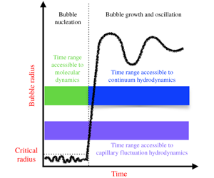
The proposed model is exploited to perform numerical simulations ranging from embryo formation up to the macroscopic oscillating motion of the bubble. A central feature of the CLLNS model is indeed its ability to bridge the gap between the nucleation phase and the successive, strongly nonlinear dynamics of the mature bubble. From the simulations the mean bubble formation time in different thermodynamic conditions is extracted and the results validated against the fully three-dimensional model. In addition, the new results are contrasted with several alternative approaches to nucleation, in particular CNT and extensions thereof, e.g. inclusion of the Tolman length to account for curvature effects on surface tension (Menzl et al. Reference Menzl, Gonzalez, Geiger, Caupin, Abascal, Valeriani and Dellago2016) and the Poynting correction to the vapour–liquid pressure difference (Angélil et al. Reference Angélil, Diemand, Tanaka and Tanaka2014). A fair comparison between models requires an accurate reconstruction of the free energy landscape. Doing so for the diffused interface approach requires the use of modern techniques. In particular, here, the string method for rare events (E, Ren & Vanden-Eijnden Reference E, Ren and Vanden-Eijnden2007) applied to the van der Waals model of the vapour–liquid system is adopted. This approach determines the minimum energy path for the transition which, coupled with Kramers theory (Kramers Reference Kramers1940), gives an alternative access to the mean first passage time, thus allowing for independent comparison with our in silico experiments based on the stochastic model. Concerning the post-critical, inertia-dominated regime, bubble oscillation dynamics is favourably compared with recent literature models for confined bubbles (Drysdale, Doinikov & Marmottant Reference Drysdale, Doinikov and Marmottant2017; Vincent & Marmottant Reference Vincent and Marmottant2017).
The structure of the paper is the following. In § 2 we discuss the mathematical aspects of the two-phase modelling. First, in § 2.1 we address the van der Waals model to describe vapour–liquid systems. In § 2.2 we retrace the FH theory in the context of the diffuse interface approach, and in § 2.3 we present the procedure to derive the spherically reduced model in detail. Section 2.4 deals with the alternative approach based on the string method, providing transition states and the minimum energy paths (MEP). Section 3 deals with the numerical simulations. More specifically, in § 3.1 we illustrate the choice of the equation of state. In § 3.2 we provide the validation of our numerics. Section 3.3 reports on the bubble nucleation results, with particular attention to mean first passage times and the eventual bubble dynamics. In § 3.4 we focus on the oscillating dynamics in a confined system. Finally § 4 is devoted to the conclusions and discusses open issues and further model development.
2 Mathematical model
2.1 Thermodynamics of liquid–vapour systems through the diffuse interface approach
Framed in the modern terminology of phase field theories (Hohenberg & Halperin Reference Hohenberg and Halperin1977), van der Waals assumed the density field as the relevant phase indicator with the squared density gradient taken as a surface penalization localized at the interface and playing the role of (distributed) surface tension (see (2.1) below). The model is extremely powerful both for steady and unsteady conditions, providing a robust description of interfacial flows that naturally accounts for topology modification of the regions occupied by the two phases and the phase change between them (Magaletti et al. Reference Magaletti, Marino and Casciola2015, Reference Magaletti, Gallo, Marino and Casciola2016). For a closed system, with a given mass  $M_{0}$, the constrained Helmholtz free energy of a two-phase flow in the van der Waals gradient approximation (Dell’Isola, Gouin & Seppecher Reference Dell’Isola, Gouin and Seppecher1995; Anderson, McFadden & Wheeler Reference Anderson, McFadden and Wheeler1998; Jamet et al. Reference Jamet, Lebaigue, Coutris and Delhaye2001) is,
 $$\begin{eqnarray}\displaystyle F_{c}[\unicode[STIX]{x1D70C},T]=\int _{V}\left(f_{b}(\unicode[STIX]{x1D70C},T)+\frac{\unicode[STIX]{x1D706}}{2}\unicode[STIX]{x1D735}\unicode[STIX]{x1D70C}\boldsymbol{\cdot }\unicode[STIX]{x1D735}\unicode[STIX]{x1D70C}\right)\,\text{d}V+l\left(M_{0}-\int _{V}\unicode[STIX]{x1D70C}\,\text{d}V\right), & & \displaystyle\end{eqnarray}$$
where  $l$ is a Lagrange multiplier and
 $f_{b}(\unicode[STIX]{x1D70C},T)$ is the classical Helmholtz free energy density per unit volume of the homogeneous fluid at temperature
 $T$ and mass density
 $\unicode[STIX]{x1D70C}$. The coefficient
 $\unicode[STIX]{x1D706}(\unicode[STIX]{x1D70C},T)$, in general a function of the thermodynamic state, is related to the interfacial properties of the liquid–vapour system, namely the surface tension and the interface thickness (see Magaletti et al. Reference Magaletti, Gallo, Marino and Casciola2016, for details). In a previous work these authors showed that a constant value for the coefficient
 $\unicode[STIX]{x1D706}$ is able to reproduce the correct temperature dependence of the surface tension (Gallo et al. Reference Gallo, Magaletti and Casciola2018b).
The model is fully specified by selecting the appropriate free energy  $f_{b}(\unicode[STIX]{x1D70C},T)$. In this work the thermodynamic properties of the fluid are described through the modified Benedict–Webb–Rubin equation of state (MBWR EoS) which mimics the behaviour of a Lennard Jones (LJ) fluid (Johnson, Zollweg & Gubbins Reference Johnson, Zollweg and Gubbins1993). The EoS directly provides the free energy
 $f_{b}$ as a function of density and temperature. Its expression is too cumbersome to be reported here, but we refer the interested reader to the original paper by Johnson et al. (Reference Johnson, Zollweg and Gubbins1993). This choice gives the opportunity for direct comparison with molecular dynamics simulations (Gallo et al. Reference Gallo, Magaletti and Casciola2018b).
At given temperature, equilibrium is characterized by the minimum of the free energy functional (2.1), where variations are performed with respect to the density distribution  $\unicode[STIX]{x1D70C}$. The resulting Euler–Lagrange equation is
 $$\begin{eqnarray}\unicode[STIX]{x1D707}_{c}^{b}-\unicode[STIX]{x1D735}\boldsymbol{\cdot }(\unicode[STIX]{x1D706}\unicode[STIX]{x1D735}\unicode[STIX]{x1D70C})-l=0,\end{eqnarray}$$
where the temperature is assumed to be constant,  $T=\text{const.}$,
 $\unicode[STIX]{x1D707}_{c}^{b}=\unicode[STIX]{x2202}f_{b}/\unicode[STIX]{x2202}\unicode[STIX]{x1D70C}|_{T}$ is the classical chemical potential and the Lagrange multiplier enforcing the mass constraint is identified as the equilibrium chemical potential,
 $l=\unicode[STIX]{x1D707}_{c}^{b}-\unicode[STIX]{x1D735}\boldsymbol{\cdot }(\unicode[STIX]{x1D706}\unicode[STIX]{x1D735}\unicode[STIX]{x1D70C})=\unicode[STIX]{x1D707}_{c}(\unicode[STIX]{x1D70C}_{eq})=\unicode[STIX]{x1D707}_{eq}$. All the functions appearing in the expression for
 $l$ are evaluated at the equilibrium density field, which is in general a function of position. The equation defines a generalized chemical potential
 $\unicode[STIX]{x1D707}_{c}=\unicode[STIX]{x1D707}_{c}^{b}-\unicode[STIX]{x1D735}\boldsymbol{\cdot }(\unicode[STIX]{x1D706}\unicode[STIX]{x1D735}\unicode[STIX]{x1D70C})$ that must be constant at equilibrium.
2.2 Fluctuating hydrodynamics: the Landau–Lifshitz/Navier–Stokes model for capillary fluids
The deterministic dynamics of the isothermal two-phase system is governed by mass and momentum conservation laws
 $$\begin{eqnarray}\displaystyle & \displaystyle {\displaystyle \frac{\unicode[STIX]{x2202}\unicode[STIX]{x1D70C}}{\unicode[STIX]{x2202}t}}+\unicode[STIX]{x1D735}\boldsymbol{\cdot }(\unicode[STIX]{x1D70C}\boldsymbol{u})=0, & \displaystyle\end{eqnarray}$$
 $$\begin{eqnarray}\displaystyle & \displaystyle {\displaystyle \frac{\unicode[STIX]{x2202}\unicode[STIX]{x1D70C}\boldsymbol{u}}{\unicode[STIX]{x2202}t}}+\unicode[STIX]{x1D735}\boldsymbol{\cdot }(\unicode[STIX]{x1D70C}\boldsymbol{u}\otimes \boldsymbol{u})=\unicode[STIX]{x1D735}\boldsymbol{\cdot }\unicode[STIX]{x1D72E}, & \displaystyle\end{eqnarray}$$
where  $\boldsymbol{u}(\boldsymbol{x},t)$ is the fluid velocity. Following the prescriptions of non-equilibrium thermodynamics (De Groot & Mazur Reference De Groot and Mazur2013), a thermodynamically consistent constitutive relationship can be found for the stress tensor
 $\unicode[STIX]{x1D72E}$. For the adopted van der Waals model (see the free energy in (2.1)) the classical stress tensor of a Newtonian fluid is augmented with capillary terms
 $$\begin{eqnarray}\unicode[STIX]{x1D72E}=\left[-p+\frac{\unicode[STIX]{x1D706}}{2}|\unicode[STIX]{x1D735}\unicode[STIX]{x1D70C}|^{2}+\unicode[STIX]{x1D706}\unicode[STIX]{x1D70C}\unicode[STIX]{x1D735}\boldsymbol{\cdot }(\unicode[STIX]{x1D706}\unicode[STIX]{x1D735}\unicode[STIX]{x1D70C})\right]\unicode[STIX]{x1D644}-\unicode[STIX]{x1D706}\unicode[STIX]{x1D735}\unicode[STIX]{x1D70C}\otimes \unicode[STIX]{x1D735}\unicode[STIX]{x1D70C}+\unicode[STIX]{x1D702}\left[(\unicode[STIX]{x1D735}\boldsymbol{u}+\unicode[STIX]{x1D735}\boldsymbol{u}^{\text{T}})-\frac{2}{3}\unicode[STIX]{x1D735}\boldsymbol{\cdot }\boldsymbol{u}\unicode[STIX]{x1D644}\right],\end{eqnarray}$$
with  $p=-\unicode[STIX]{x1D70C}^{2}\unicode[STIX]{x2202}(f_{b}/\unicode[STIX]{x1D70C})/\unicode[STIX]{x2202}\unicode[STIX]{x1D70C}=f_{b}-\unicode[STIX]{x1D707}_{c}^{b}\unicode[STIX]{x1D70C}$ the pressure and
 $\unicode[STIX]{x1D702}$ the dynamic viscosity, (Jamet et al. Reference Jamet, Lebaigue, Coutris and Delhaye2001; Magaletti et al. Reference Magaletti, Gallo, Marino and Casciola2016).
Thermal fluctuations can be consistently embedded into the diffuse interface model in the spirit of FH (Gallo et al. Reference Gallo, Magaletti and Casciola2018b). FH is a stochastic fluid model originally proposed in the pioneering work of Landau & Lifshitz (Reference Landau and Lifshitz1958) and systematically derived in Fox & Uhlenbeck (Reference Fox and Uhlenbeck1970) for simple Newtonian fluids. The basic assumption is that fluctuations can be described by the usual hydrodynamic equations once supplemented with random noise terms whose statistical properties are inferred by enforcing the fluctuation–dissipation balance (FDB). The random noise force is represented by the divergence of a stochastic stress tensor  $\unicode[STIX]{x1D739}\unicode[STIX]{x1D72E}$, a zero mean Gaussian process characterized below, which adds to the ordinary momentum balance equation
 $$\begin{eqnarray}{\displaystyle \frac{\unicode[STIX]{x2202}\unicode[STIX]{x1D70C}\boldsymbol{u}}{\unicode[STIX]{x2202}t}}+\unicode[STIX]{x1D735}\boldsymbol{\cdot }(\unicode[STIX]{x1D70C}\boldsymbol{u}\otimes \boldsymbol{u})=\unicode[STIX]{x1D735}\boldsymbol{\cdot }\unicode[STIX]{x1D72E}+\unicode[STIX]{x1D735}\boldsymbol{\cdot }\unicode[STIX]{x1D739}\unicode[STIX]{x1D72E}.\end{eqnarray}$$
Enforcing the fluctuation–dissipation balance, the covariance of the stochastic tensor reads (in components)
 $$\begin{eqnarray}\langle \unicode[STIX]{x1D6FF}\unicode[STIX]{x1D6F4}_{\unicode[STIX]{x1D6FC}\unicode[STIX]{x1D6FD}}(\hat{\boldsymbol{x}},\hat{t})\otimes \unicode[STIX]{x1D6FF}\unicode[STIX]{x1D6F4}_{\unicode[STIX]{x1D708}\unicode[STIX]{x1D702}}(\tilde{\boldsymbol{x}},\tilde{t})\rangle =2\text{k}_{B}T\unicode[STIX]{x1D702}(\unicode[STIX]{x1D6FF}_{\unicode[STIX]{x1D6FC}\unicode[STIX]{x1D708}}\unicode[STIX]{x1D6FF}_{\unicode[STIX]{x1D6FD}\unicode[STIX]{x1D702}}+\unicode[STIX]{x1D6FF}_{\unicode[STIX]{x1D6FC}\unicode[STIX]{x1D702}}\unicode[STIX]{x1D6FF}_{\unicode[STIX]{x1D6FD}\unicode[STIX]{x1D708}}-{\textstyle \frac{2}{3}}\unicode[STIX]{x1D6FF}_{\unicode[STIX]{x1D6FC}\unicode[STIX]{x1D6FD}}\unicode[STIX]{x1D6FF}_{\unicode[STIX]{x1D708}\unicode[STIX]{x1D702}})\unicode[STIX]{x1D6FF}(\hat{\boldsymbol{x}}-\tilde{\boldsymbol{x}})\unicode[STIX]{x1D6FF}(\hat{t}-\tilde{t}),\end{eqnarray}$$
with  $\text{k}_{B}$ the Boltzmann constant. As a consequence of the stochastic force, the hydrodynamic fields (namely density and velocity) fluctuate.
The equilibrium correlation tensor  $\unicode[STIX]{x1D63E}_{\unicode[STIX]{x1D71F}}(\hat{\boldsymbol{x}},\tilde{\boldsymbol{x}})=\langle \unicode[STIX]{x1D71F}(\hat{\boldsymbol{x}})\otimes \unicode[STIX]{x1D71F}^{\dagger }(\tilde{\boldsymbol{x}})\rangle$ of the field fluctuations, organized in a 4-component vector
 $\unicode[STIX]{x1D71F}(\boldsymbol{x})=\{\unicode[STIX]{x1D6FF}\unicode[STIX]{x1D70C}(\boldsymbol{x}),\unicode[STIX]{x1D739}\boldsymbol{u}(\boldsymbol{x})\}$, is found to be (Gallo et al. Reference Gallo, Magaletti and Casciola2018b)
 $$\begin{eqnarray}\unicode[STIX]{x1D63E}_{\unicode[STIX]{x1D71F}}(\hat{\boldsymbol{r}},\tilde{\boldsymbol{r}})=\left(\begin{array}{@{}cc@{}}C_{\unicode[STIX]{x1D6FF}\unicode[STIX]{x1D70C}\unicode[STIX]{x1D6FF}\unicode[STIX]{x1D70C}} & 0\\ 0 & \unicode[STIX]{x1D63E}_{\unicode[STIX]{x1D6FF}\boldsymbol{ u}\unicode[STIX]{x1D6FF}\boldsymbol{u}}\end{array}\right),\end{eqnarray}$$
with
 $$\begin{eqnarray}\displaystyle & \displaystyle C_{\unicode[STIX]{x1D6FF}\unicode[STIX]{x1D70C}\unicode[STIX]{x1D6FF}\unicode[STIX]{x1D70C}}(\hat{\boldsymbol{r}},\tilde{\boldsymbol{r}})=\frac{\text{k}_{B}T_{0}}{4\unicode[STIX]{x03C0}\unicode[STIX]{x1D706}|\hat{\boldsymbol{r}}-\tilde{\boldsymbol{r}}|}\exp \left(-|\hat{\boldsymbol{r}}-\tilde{\boldsymbol{r}}|\sqrt{\frac{c_{T}^{2}}{\unicode[STIX]{x1D70C}_{0}\unicode[STIX]{x1D706}}}\right), & \displaystyle\end{eqnarray}$$
 $$\begin{eqnarray}\displaystyle & \displaystyle \unicode[STIX]{x1D63E}_{\unicode[STIX]{x1D6FF}\boldsymbol{u}\unicode[STIX]{x1D6FF}\boldsymbol{u}}(\hat{\boldsymbol{r}},\tilde{\boldsymbol{r}})=\frac{\text{k}_{B}T_{0}}{\unicode[STIX]{x1D70C}_{0}}\unicode[STIX]{x1D644}\unicode[STIX]{x1D6FF}(\hat{\boldsymbol{r}}-\tilde{\boldsymbol{r}}). & \displaystyle\end{eqnarray}$$
In the above equation,  $\unicode[STIX]{x1D70C}_{0}$ and
 $T_{0}$ are the equilibrium density and temperature, respectively, and
 $c_{T}^{2}=\unicode[STIX]{x2202}p/\unicode[STIX]{x2202}\unicode[STIX]{x1D70C}|_{T}$ is the isothermal speed of sound. At variance with the usual
 $\unicode[STIX]{x1D6FF}$-correlation typical of simple fluids (De Zarate & Sengers Reference De Zarate and Sengers2006), the exponential decay of the density fluctuation spatial correlation arises from the long range capillary interactions.
2.3 The spherically reduced model
With the aim of reproducing the most relevant features of bubble nucleation in a simplified setting, a reduced model is here derived under the assumption of spherical symmetry. As discussed in the Introduction, a systematic procedure has been proposed by Lutsko (Reference Lutsko2012) in the case of a diffusive dynamics of a spherical colloid in the overdamped limit. This methodology requires the complete dynamical equations to be averaged on a spherical shell in order to obtain a set of evolution stochastic equations spatially depending only on the radial distance from the cluster centre. The averaging procedure transforms the full three-dimensional stochastic fields  $\unicode[STIX]{x1D70C}(\boldsymbol{x},t)$ and
 $\boldsymbol{u}(\boldsymbol{x},t)$ in the purely radial quantities
 $\bar{\unicode[STIX]{x1D70C}}(r,t)$ and
 $\bar{u}_{r}(r,t)$. The assumption of spherical symmetry is the delicate point of the procedure since the random stresses are expected to break this symmetry. The idea is to find an expression for an equivalent stochastic force, depending only on the radial coordinate, which recovers exactly the statistical properties of the original spherically averaged noise.
Before concentrating on the technical details, some general discussion is worthwhile. The theory of fluctuating hydrodynamics was originally formulated to deal with fluctuations in fluids in thermodynamic equilibrium. The typical derivation of the FDB is obtained based on linear equations, i.e. under the assumption of small fluctuations with respect to the equilibrium values, see Español, Serrano & Öttinger (Reference Español, Serrano and Öttinger1999) and Español, Anero & Zúñiga (Reference Español, Anero and Zúñiga2009) for a more general derivation of the very same model in the nonlinear context. The common approach when dealing with non-equilibrium states is based on the assumption that the correlations of the fluctuating fields obey a local-equilibrium version of the FDB (De Zarate & Sengers Reference De Zarate and Sengers2006). This should not sound unfamiliar since it is the usual way to proceed in non-equilibrium thermodynamics (De Groot & Mazur Reference De Groot and Mazur2013), where the equilibrium laws, such as  $p=p(\unicode[STIX]{x1D70C},T)$, continue to hold for the locally defined fluid properties,
 $p(\boldsymbol{x},t)=p(\unicode[STIX]{x1D70C}(\boldsymbol{x},t),T(\boldsymbol{x},t))$. It is worth noticing that similar assumptions are necessary also in more fundamental approaches such as dynamic density functional theory (Archer Reference Archer2009; Goddard et al. Reference Goddard, Nold, Savva, Yatsyshin and Kalliadasis2012). The fact that the FDB is local means that the correlation of the random stress tensor is obtained by substituting the local temperature and viscosity in (2.7). In the spirit of FH we formally apply the averaging procedure to the linearized version of the equations to obtain the expression of the equivalent radial stochastic force in a fluid in equilibrium. Successively, under the common assumption of local equilibrium, we extend the obtained expression to non-equilibrium, nonlinear, conditions.
Let us define  $\unicode[STIX]{x1D70C}^{\prime }$ and
 $\boldsymbol{u}^{\prime }$, the small fluctuations of the density and velocity, respectively, around their equilibrium values,
 $\unicode[STIX]{x1D70C}_{0}$ and
 $\boldsymbol{u}_{\mathbf{0}}=\mathbf{0}$. The linearized version of the continuity equation, equation (2.3), in spherical coordinates reads as
 $$\begin{eqnarray}\frac{\unicode[STIX]{x2202}\unicode[STIX]{x1D70C}^{\prime }}{\unicode[STIX]{x2202}t}+\unicode[STIX]{x1D70C}_{0}\left[\frac{1}{r^{2}}\frac{\unicode[STIX]{x2202}}{\unicode[STIX]{x2202}r}(r^{2}u_{r}^{\prime })+\frac{1}{r\sin \unicode[STIX]{x1D703}}\frac{\unicode[STIX]{x2202}}{\unicode[STIX]{x2202}\unicode[STIX]{x1D703}}(u_{\unicode[STIX]{x1D703}}^{\prime }\sin \unicode[STIX]{x1D703})+\frac{1}{r\sin \unicode[STIX]{x1D703}}\frac{\unicode[STIX]{x2202}}{\unicode[STIX]{x2202}\unicode[STIX]{x1D711}}(u_{\unicode[STIX]{x1D711}}^{\prime })\right]=0.\end{eqnarray}$$
In order to evaluate the evolution of the averaged density over the surface of a sphere with radius  $r$, we apply the spherical averaging operator
 ${\mathcal{M}}$, defined on the generic field
 $g(r,\unicode[STIX]{x1D703},\unicode[STIX]{x1D711},t)$ as
 $$\begin{eqnarray}{\mathcal{M}}[g](r,t)=\frac{1}{4\unicode[STIX]{x03C0}}\int _{0}^{\unicode[STIX]{x03C0}}\int _{0}^{2\unicode[STIX]{x03C0}}g\sin \unicode[STIX]{x1D703}\,\text{d}\unicode[STIX]{x1D703}\,\text{d}\unicode[STIX]{x1D711}.\end{eqnarray}$$
We thus obtain an evolution equation for the spherically averaged density  $\bar{\unicode[STIX]{x1D70C}}={\mathcal{M}}[\unicode[STIX]{x1D70C}^{\prime }]$
 $$\begin{eqnarray}\frac{\unicode[STIX]{x2202}\bar{\unicode[STIX]{x1D70C}}}{\unicode[STIX]{x2202}t}=-\unicode[STIX]{x1D70C}_{0}{\mathcal{M}}\left[\frac{1}{r^{2}}\frac{\unicode[STIX]{x2202}}{\unicode[STIX]{x2202}r}(r^{2}u_{r}^{\prime })+\frac{1}{r\sin \unicode[STIX]{x1D703}}\frac{\unicode[STIX]{x2202}}{\unicode[STIX]{x2202}\unicode[STIX]{x1D703}}(u_{\unicode[STIX]{x1D703}}^{\prime }\sin \unicode[STIX]{x1D703})+\frac{1}{r\sin \unicode[STIX]{x1D703}}\frac{\unicode[STIX]{x2202}}{\unicode[STIX]{x2202}\unicode[STIX]{x1D711}}(u_{\unicode[STIX]{x1D711}}^{\prime })\right]=-\unicode[STIX]{x1D70C}_{0}\frac{1}{r^{2}}\frac{\unicode[STIX]{x2202}}{\unicode[STIX]{x2202}r}(r^{2}\bar{u}_{r}),\end{eqnarray}$$
where  $\bar{u}_{r}(r,t)$ is the averaged radial velocity and the other two contributions vanish after integration. It worth noticing that the averaged density evolution is only affected by the radial velocity. This suggests that we apply the same averaging operator to the radial component of the linearized momentum equation, again in spherical coordinates
 $$\begin{eqnarray}\displaystyle \unicode[STIX]{x1D70C}_{0}\frac{\unicode[STIX]{x2202}\bar{u}_{r}}{\unicode[STIX]{x2202}t} & = & \displaystyle {\mathcal{M}}\left[\frac{1}{r^{2}}\frac{\unicode[STIX]{x2202}}{\unicode[STIX]{x2202}r}(r^{2}\unicode[STIX]{x1D6F4}_{rr}^{L})+\frac{1}{r\sin \unicode[STIX]{x1D703}}\frac{\unicode[STIX]{x2202}}{\unicode[STIX]{x2202}\unicode[STIX]{x1D703}}(\unicode[STIX]{x1D6F4}_{r\unicode[STIX]{x1D703}}^{L}\sin \unicode[STIX]{x1D703})+\frac{1}{r\sin \unicode[STIX]{x1D703}}\frac{\unicode[STIX]{x2202}}{\unicode[STIX]{x2202}\unicode[STIX]{x1D711}}(\unicode[STIX]{x1D6F4}_{r\unicode[STIX]{x1D711}}^{L})-\frac{\unicode[STIX]{x1D6F4}_{\unicode[STIX]{x1D703}\unicode[STIX]{x1D703}}^{L}+\unicode[STIX]{x1D6F4}_{\unicode[STIX]{x1D711}\unicode[STIX]{x1D711}}^{L}}{r}\right]\nonumber\\ \displaystyle & = & \displaystyle {\mathcal{M}}\left[\frac{1}{r^{2}}\frac{\unicode[STIX]{x2202}}{\unicode[STIX]{x2202}r}(r^{2}\unicode[STIX]{x1D6F4}_{rr}^{L})-\frac{\unicode[STIX]{x1D6F4}_{\unicode[STIX]{x1D703}\unicode[STIX]{x1D703}}^{L}+\unicode[STIX]{x1D6F4}_{\unicode[STIX]{x1D711}\unicode[STIX]{x1D711}}^{L}}{r}\right]=\unicode[STIX]{x1D6E4}_{r}^{L}+\unicode[STIX]{x1D6FF}\unicode[STIX]{x1D6E4}_{r},\end{eqnarray}$$
where the stress tensor  $\unicode[STIX]{x1D72E}^{L}$ appearing in the above equation is the linearized total stress tensor consisting of both the deterministic and stochastic contributions
 $$\begin{eqnarray}\unicode[STIX]{x1D72E}^{L}=(-c_{T}^{2}\unicode[STIX]{x1D70C}^{\prime }+\unicode[STIX]{x1D706}\unicode[STIX]{x1D70C}_{0}\unicode[STIX]{x1D6FB}^{2}\unicode[STIX]{x1D70C}^{\prime })\unicode[STIX]{x1D644}+\unicode[STIX]{x1D702}_{0}(\unicode[STIX]{x1D735}\boldsymbol{u}^{\prime }+\unicode[STIX]{x1D735}{\boldsymbol{u}^{\prime }}^{\text{T}}-{\textstyle \frac{2}{3}}\unicode[STIX]{x1D735}\boldsymbol{\cdot }\boldsymbol{u}^{\prime }\unicode[STIX]{x1D644})+\unicode[STIX]{x1D739}\unicode[STIX]{x1D72E}.\end{eqnarray}$$
Here,  $\unicode[STIX]{x1D6E4}_{r}^{L}$ and
 $\unicode[STIX]{x1D6FF}\unicode[STIX]{x1D6E4}_{r}$ denote the spherically averaged deterministic and stochastic radial forces, respectively. In the definition of the linearized stress tensor,
 $c_{T}^{2}$ represents the square of the isothermal speed of sound evaluated at the reference condition
 $\unicode[STIX]{x1D70C}_{0}$. The relevant components of the linearized stress tensor are readily obtained,
 $$\begin{eqnarray}\displaystyle & \displaystyle \unicode[STIX]{x1D6F4}_{rr}^{L}=-c_{T}^{2}\unicode[STIX]{x1D70C}^{\prime }+\frac{\unicode[STIX]{x1D706}\unicode[STIX]{x1D70C}_{0}}{r^{2}}\frac{\unicode[STIX]{x2202}}{\unicode[STIX]{x2202}r}\left(r^{2}\frac{\unicode[STIX]{x2202}\unicode[STIX]{x1D70C}^{\prime }}{\unicode[STIX]{x2202}r}\right)+2\unicode[STIX]{x1D702}_{0}\left[\frac{\unicode[STIX]{x2202}u_{r}^{\prime }}{\unicode[STIX]{x2202}r}-\frac{1}{3}\unicode[STIX]{x1D735}\boldsymbol{\cdot }\boldsymbol{u}^{\prime }\right]+\unicode[STIX]{x1D6FF}\unicode[STIX]{x1D6F4}_{rr}, & \displaystyle\end{eqnarray}$$
 $$\begin{eqnarray}\displaystyle & \displaystyle \unicode[STIX]{x1D6F4}_{\unicode[STIX]{x1D703}\unicode[STIX]{x1D703}}^{L}=-c_{T}^{2}\unicode[STIX]{x1D70C}^{\prime }+\frac{\unicode[STIX]{x1D706}\unicode[STIX]{x1D70C}_{0}}{r^{2}}\frac{\unicode[STIX]{x2202}}{\unicode[STIX]{x2202}r}\left(r^{2}\frac{\unicode[STIX]{x2202}\unicode[STIX]{x1D70C}^{\prime }}{\unicode[STIX]{x2202}r}\right)+2\unicode[STIX]{x1D702}_{0}\left[\frac{u_{r}^{\prime }}{r}-\frac{1}{3}\unicode[STIX]{x1D735}\boldsymbol{\cdot }\boldsymbol{u}^{\prime }\right]+\unicode[STIX]{x1D6FF}\unicode[STIX]{x1D6F4}_{\unicode[STIX]{x1D703}\unicode[STIX]{x1D703}}, & \displaystyle\end{eqnarray}$$
 $$\begin{eqnarray}\displaystyle & \displaystyle \unicode[STIX]{x1D6F4}_{\unicode[STIX]{x1D711}\unicode[STIX]{x1D711}}^{L}=-c_{T}^{2}\unicode[STIX]{x1D70C}^{\prime }+\frac{\unicode[STIX]{x1D706}\unicode[STIX]{x1D70C}_{0}}{r^{2}}\frac{\unicode[STIX]{x2202}}{\unicode[STIX]{x2202}r}\left(r^{2}\frac{\unicode[STIX]{x2202}\unicode[STIX]{x1D70C}^{\prime }}{\unicode[STIX]{x2202}r}\right)+2\unicode[STIX]{x1D702}_{0}\left[\frac{u_{r}^{\prime }}{r}-\frac{1}{3}\unicode[STIX]{x1D735}\boldsymbol{\cdot }\boldsymbol{u}^{\prime }\right]+\unicode[STIX]{x1D6FF}\unicode[STIX]{x1D6F4}_{\unicode[STIX]{x1D711}\unicode[STIX]{x1D711}}. & \displaystyle\end{eqnarray}$$
When the averaging operator is applied to the deterministic contributions, the radial force is found to be
 $$\begin{eqnarray}\displaystyle \unicode[STIX]{x1D6E4}_{r}^{L} & = & \displaystyle \frac{\unicode[STIX]{x2202}}{\unicode[STIX]{x2202}r}\left[-c_{T}^{2}\bar{\unicode[STIX]{x1D70C}}+\frac{\unicode[STIX]{x1D706}\unicode[STIX]{x1D70C}_{0}}{r^{2}}\frac{\unicode[STIX]{x2202}}{\unicode[STIX]{x2202}r}\left(r^{2}\frac{\unicode[STIX]{x2202}\bar{\unicode[STIX]{x1D70C}}}{\unicode[STIX]{x2202}r}\right)-\frac{2\unicode[STIX]{x1D702}_{0}}{3}\frac{1}{r^{2}}\frac{\unicode[STIX]{x2202}}{\unicode[STIX]{x2202}r}(r^{2}\bar{u}_{r})\right]\nonumber\\ \displaystyle & & \displaystyle +\,\frac{2\unicode[STIX]{x1D702}_{0}}{r^{2}}\frac{\unicode[STIX]{x2202}}{\unicode[STIX]{x2202}r}\left(r^{2}\frac{\unicode[STIX]{x2202}\bar{u}_{r}}{\unicode[STIX]{x2202}r}\right)-\frac{4\unicode[STIX]{x1D702}_{0}\bar{u}_{r}}{r^{2}}.\end{eqnarray}$$
The correlation tensor given in (2.7), expressing the correlation of the Cartesian components (with respect to the basis  ${\mathcal{B}}=\{\boldsymbol{e}_{x},\boldsymbol{e}_{y},\boldsymbol{e}_{z}\}$) of the stochastic stress tensor, can be converted into the spherical-polar basis
 ${\mathcal{B}}^{S}=\{\boldsymbol{e}_{r},\boldsymbol{e}_{\unicode[STIX]{x1D703}},\boldsymbol{e}_{\unicode[STIX]{x1D711}}\}$ by applying the classical orthogonal transformation
 $$\begin{eqnarray}\unicode[STIX]{x1D6FF}\unicode[STIX]{x1D6F4}_{pq}=B_{pk}^{{\mathcal{B}}^{S}\rightarrow {\mathcal{B}}}B_{ql}^{{\mathcal{B}}^{S}\rightarrow {\mathcal{B}}}\unicode[STIX]{x1D6FF}\unicode[STIX]{x1D6F4}_{kl},\end{eqnarray}$$
with the index set  $p,q=\{r,\unicode[STIX]{x1D703},\unicode[STIX]{x1D711}\}$ and
 $k,l=\{x,y,z\}$. The transformation matrix
 $\unicode[STIX]{x1D63D}^{{\mathcal{B}}^{S}\rightarrow {\mathcal{B}}}$ is the orthogonal (
 $3\times 3$) matrix whose entries are
 $$\begin{eqnarray}\displaystyle \unicode[STIX]{x1D63D}_{{\mathcal{B}}^{S}\rightarrow {\mathcal{B}}}=\left(\begin{array}{@{}ccc@{}}\sin \unicode[STIX]{x1D703}\cos \unicode[STIX]{x1D711} & \sin \unicode[STIX]{x1D703}\sin \unicode[STIX]{x1D711} & \cos \unicode[STIX]{x1D703}\\ \cos \unicode[STIX]{x1D703}\cos \unicode[STIX]{x1D711} & \cos \unicode[STIX]{x1D703}\sin \unicode[STIX]{x1D711} & -\text{sin}\,\unicode[STIX]{x1D703}\\ -\text{sin}\,\unicode[STIX]{x1D711} & \cos \unicode[STIX]{x1D711} & 0\end{array}\right), & & \displaystyle\end{eqnarray}$$
accomplishing the coordinate transformation by rotating the Cartesian basis, i.e.  $\unicode[STIX]{x1D609}_{ik}^{{\mathcal{B}}^{S}\rightarrow {\mathcal{B}}}\unicode[STIX]{x1D609}_{jk}^{{\mathcal{B}}^{S}\rightarrow {\mathcal{B}}}=\unicode[STIX]{x1D6FF}_{ij}$. By applying the rules in (2.20), the correlation tensor has the form
 $$\begin{eqnarray}\langle \unicode[STIX]{x1D6FF}\unicode[STIX]{x1D6F4}_{mn}(\hat{\boldsymbol{x}},\hat{t})\unicode[STIX]{x1D6FF}\unicode[STIX]{x1D6F4}_{pq}(\tilde{\boldsymbol{x}},\tilde{t})\rangle ={\mathcal{I}}(\unicode[STIX]{x1D6FF}_{mp}\unicode[STIX]{x1D6FF}_{nq}+\unicode[STIX]{x1D6FF}_{mq}\unicode[STIX]{x1D6FF}_{np}-{\textstyle \frac{2}{3}}\unicode[STIX]{x1D6FF}_{mn}\unicode[STIX]{x1D6FF}_{pq}),\end{eqnarray}$$
with  ${\mathcal{I}}=2\unicode[STIX]{x1D702}\text{k}_{B}T\unicode[STIX]{x1D6FF}(\hat{r}-\tilde{r})\unicode[STIX]{x1D6FF}(\hat{\unicode[STIX]{x1D703}}-\tilde{\unicode[STIX]{x1D703}})\unicode[STIX]{x1D6FF}(\hat{\unicode[STIX]{x1D711}}-\tilde{\unicode[STIX]{x1D711}})\unicode[STIX]{x1D6FF}(\hat{t}-\tilde{t})/(\hat{r}^{2}\sin \hat{\unicode[STIX]{x1D703}})$, and
 $m,n,p,q=r,\unicode[STIX]{x1D703},\unicode[STIX]{x1D711}$, where the Jacobian
 $\hat{r}^{2}\sin \hat{\unicode[STIX]{x1D703}}$ appears due to the expression in spherical coordinates of the original Dirac delta function in Cartesian variables. Explicitly, the relevant correlations are
 $$\begin{eqnarray}\displaystyle & \displaystyle \langle \unicode[STIX]{x1D6FF}\unicode[STIX]{x1D6F4}_{rr}(\hat{\boldsymbol{x}},\hat{t})\unicode[STIX]{x1D6FF}\unicode[STIX]{x1D6F4}_{rr}(\tilde{\boldsymbol{x}},\tilde{t})\rangle =\langle \unicode[STIX]{x1D6FF}\unicode[STIX]{x1D6F4}_{\unicode[STIX]{x1D703}\unicode[STIX]{x1D703}}(\hat{\boldsymbol{x}},\hat{t})\unicode[STIX]{x1D6FF}\unicode[STIX]{x1D6F4}_{\unicode[STIX]{x1D703}\unicode[STIX]{x1D703}}(\tilde{\boldsymbol{x}},\tilde{t})\rangle =\langle \unicode[STIX]{x1D6FF}\unicode[STIX]{x1D6F4}_{\unicode[STIX]{x1D711}\unicode[STIX]{x1D711}}(\hat{\boldsymbol{x}},\hat{t})\unicode[STIX]{x1D6FF}\unicode[STIX]{x1D6F4}_{\unicode[STIX]{x1D711}\unicode[STIX]{x1D711}}(\tilde{\boldsymbol{x}},\tilde{t})\rangle ={\textstyle \frac{4}{3}}{\mathcal{I}},\qquad & \displaystyle\end{eqnarray}$$
 $$\begin{eqnarray}\displaystyle & \displaystyle \langle \unicode[STIX]{x1D6FF}\unicode[STIX]{x1D6F4}_{rr}(\hat{\boldsymbol{x}},\hat{t})\unicode[STIX]{x1D6FF}\unicode[STIX]{x1D6F4}_{\unicode[STIX]{x1D703}\unicode[STIX]{x1D703}}(\tilde{\boldsymbol{x}},\tilde{t})\rangle =\langle \unicode[STIX]{x1D6FF}\unicode[STIX]{x1D6F4}_{rr}(\hat{\boldsymbol{x}},\hat{t})\unicode[STIX]{x1D6FF}\unicode[STIX]{x1D6F4}_{\unicode[STIX]{x1D711}\unicode[STIX]{x1D711}}(\tilde{\boldsymbol{x}},\tilde{t})\rangle =\langle \unicode[STIX]{x1D6FF}\unicode[STIX]{x1D6F4}_{\unicode[STIX]{x1D703}\unicode[STIX]{x1D703}}(\hat{\boldsymbol{x}},\hat{t})\unicode[STIX]{x1D6FF}\unicode[STIX]{x1D6F4}_{\unicode[STIX]{x1D711}\unicode[STIX]{x1D711}}(\tilde{\boldsymbol{x}},\tilde{t})\rangle =-{\textstyle \frac{2}{3}}{\mathcal{I}}.\qquad & \displaystyle\end{eqnarray}$$
Since both  $\unicode[STIX]{x1D6FF}\unicode[STIX]{x1D6F4}_{\unicode[STIX]{x1D703}\unicode[STIX]{x1D703}}$ and
 $\unicode[STIX]{x1D6FF}\unicode[STIX]{x1D6F4}_{\unicode[STIX]{x1D711}\unicode[STIX]{x1D711}}$ are Gaussian processes with correlations given by (2.23), (2.24), their sum is also a Gaussian process
 $\unicode[STIX]{x1D6FF}\unicode[STIX]{x1D6F4}_{\unicode[STIX]{x1D719}\unicode[STIX]{x1D719}}=\unicode[STIX]{x1D6FF}\unicode[STIX]{x1D6F4}_{\unicode[STIX]{x1D703}\unicode[STIX]{x1D703}}+\unicode[STIX]{x1D6FF}\unicode[STIX]{x1D6F4}_{\unicode[STIX]{x1D711}\unicode[STIX]{x1D711}}$ with autocorrelation
 $\langle \unicode[STIX]{x1D6FF}\unicode[STIX]{x1D6F4}_{\unicode[STIX]{x1D719}\unicode[STIX]{x1D719}}(\hat{\boldsymbol{x}},\hat{t})\unicode[STIX]{x1D6FF}\unicode[STIX]{x1D6F4}_{\unicode[STIX]{x1D719}\unicode[STIX]{x1D719}}(\tilde{\boldsymbol{x}},\tilde{t})\rangle =4/3{\mathcal{I}}$ and cross-correlation
 $\langle \unicode[STIX]{x1D6FF}\unicode[STIX]{x1D6F4}_{\unicode[STIX]{x1D719}\unicode[STIX]{x1D719}}(\hat{\boldsymbol{x}},\hat{t})\unicode[STIX]{x1D6FF}\unicode[STIX]{x1D6F4}_{rr}(\tilde{\boldsymbol{x}},\tilde{t})\rangle =-4/3{\mathcal{I}}$. By applying the averaging operator
 ${\mathcal{M}}$ one may then obtain the correlation of the averaged radial stochastic force, namely,
 $$\begin{eqnarray}\langle \unicode[STIX]{x1D6FF}\unicode[STIX]{x1D6E4}_{r}(\hat{r},\hat{t})\unicode[STIX]{x1D6FF}\unicode[STIX]{x1D6E4}_{r}(\tilde{r},\tilde{t})\rangle =\left\langle {\mathcal{M}}\left[\frac{1}{\hat{r}^{2}}\frac{\unicode[STIX]{x2202}}{\unicode[STIX]{x2202}\hat{r}}(\hat{r}^{2}\unicode[STIX]{x1D6FF}\unicode[STIX]{x1D6F4}_{rr})-\frac{\unicode[STIX]{x1D6FF}\unicode[STIX]{x1D6F4}_{\unicode[STIX]{x1D719}\unicode[STIX]{x1D719}}}{\hat{r}}\right]{\mathcal{M}}\left[\frac{1}{\tilde{r}^{2}}\frac{\unicode[STIX]{x2202}}{\unicode[STIX]{x2202}\tilde{r}}(\tilde{r}^{2}\unicode[STIX]{x1D6FF}\unicode[STIX]{x1D6F4}_{rr})-\frac{\unicode[STIX]{x1D6FF}\unicode[STIX]{x1D6F4}_{\unicode[STIX]{x1D719}\unicode[STIX]{x1D719}}}{\tilde{r}}\right]\right\rangle .\end{eqnarray}$$
Since the operator  ${\mathcal{M}}$ does not depend on the radial coordinate, it commutes with the radial derivative and directly applies to the two components of the stress tensor
 $\unicode[STIX]{x1D6FF}\unicode[STIX]{x1D6F4}_{rr}$ and
 $\unicode[STIX]{x1D6FF}\unicode[STIX]{x1D6F4}_{\unicode[STIX]{x1D719}\unicode[STIX]{x1D719}}$
 $$\begin{eqnarray}\displaystyle & & \displaystyle \langle \unicode[STIX]{x1D6FF}\unicode[STIX]{x1D6E4}_{r}(\hat{r},\hat{t})\unicode[STIX]{x1D6FF}\unicode[STIX]{x1D6E4}_{r}(\tilde{r},\tilde{t})\rangle \nonumber\\ \displaystyle & & \displaystyle \quad =\frac{1}{(4\unicode[STIX]{x03C0})^{2}\hat{r}^{2}\tilde{r}^{2}}\frac{\unicode[STIX]{x2202}^{2}}{\unicode[STIX]{x2202}\hat{r}\unicode[STIX]{x2202}\tilde{r}}\left[\hat{r}^{2}\tilde{r}^{2}\int _{0}^{\unicode[STIX]{x03C0}}\int _{0}^{\unicode[STIX]{x03C0}}\int _{0}^{2\unicode[STIX]{x03C0}}\int _{0}^{2\unicode[STIX]{x03C0}}\langle \unicode[STIX]{x1D6FF}\unicode[STIX]{x1D6F4}_{rr}\unicode[STIX]{x1D6FF}\unicode[STIX]{x1D6F4}_{rr}\rangle \sin \hat{\unicode[STIX]{x1D703}}\sin \tilde{\unicode[STIX]{x1D703}}\,\text{d}\hat{\unicode[STIX]{x1D703}}\,\text{d}\tilde{\unicode[STIX]{x1D703}}\,\text{d}\hat{\unicode[STIX]{x1D711}}\,\text{d}\tilde{\unicode[STIX]{x1D711}}\right]\nonumber\\ \displaystyle & & \displaystyle \qquad +\,\frac{2}{(4\unicode[STIX]{x03C0})^{2}\hat{r}^{2}\tilde{r}}\frac{\unicode[STIX]{x2202}}{\unicode[STIX]{x2202}\hat{r}}\left[\hat{r}^{2}\int _{0}^{\unicode[STIX]{x03C0}}\int _{0}^{\unicode[STIX]{x03C0}}\int _{0}^{2\unicode[STIX]{x03C0}}\int _{0}^{2\unicode[STIX]{x03C0}}\langle \unicode[STIX]{x1D6FF}\unicode[STIX]{x1D6F4}_{rr}\unicode[STIX]{x1D6FF}\unicode[STIX]{x1D6F4}_{\unicode[STIX]{x1D719}\unicode[STIX]{x1D719}}\rangle \sin \hat{\unicode[STIX]{x1D703}}\sin \tilde{\unicode[STIX]{x1D703}}\,\text{d}\hat{\unicode[STIX]{x1D703}}\,\text{d}\tilde{\unicode[STIX]{x1D703}}\,\text{d}\hat{\unicode[STIX]{x1D711}}\,\text{d}\tilde{\unicode[STIX]{x1D711}}\right]\nonumber\\ \displaystyle & & \displaystyle \qquad +\,\frac{1}{(4\unicode[STIX]{x03C0})^{2}\hat{r}\tilde{r}}\int _{0}^{\unicode[STIX]{x03C0}}\int _{0}^{\unicode[STIX]{x03C0}}\int _{0}^{2\unicode[STIX]{x03C0}}\int _{0}^{2\unicode[STIX]{x03C0}}\langle \unicode[STIX]{x1D6FF}\unicode[STIX]{x1D6F4}_{\unicode[STIX]{x1D719}\unicode[STIX]{x1D719}}\unicode[STIX]{x1D6FF}\unicode[STIX]{x1D6F4}_{\unicode[STIX]{x1D719}\unicode[STIX]{x1D719}}\rangle \sin \hat{\unicode[STIX]{x1D703}}\sin \tilde{\unicode[STIX]{x1D703}}\,\text{d}\hat{\unicode[STIX]{x1D703}}\,\text{d}\tilde{\unicode[STIX]{x1D703}}\,\text{d}\hat{\unicode[STIX]{x1D711}}\,\text{d}\tilde{\unicode[STIX]{x1D711}}.\end{eqnarray}$$
After some algebra one finds
 $$\begin{eqnarray}\displaystyle & & \displaystyle \langle \unicode[STIX]{x1D6FF}\unicode[STIX]{x1D6E4}_{r}(\hat{r},\hat{t})\unicode[STIX]{x1D6FF}\unicode[STIX]{x1D6E4}_{r}(\tilde{r},\tilde{t})\rangle \nonumber\\ \displaystyle & & \displaystyle \quad ={\mathcal{Z}}\left\{\frac{1}{\hat{r}^{2}\tilde{r}^{2}}\frac{\unicode[STIX]{x2202}^{2}}{\unicode[STIX]{x2202}\hat{r}\unicode[STIX]{x2202}\tilde{r}}[\hat{r}^{2}\unicode[STIX]{x1D6FF}(\hat{r}-\tilde{r})]+2\frac{1}{\hat{r}^{2}\tilde{r}}\frac{\unicode[STIX]{x2202}}{\unicode[STIX]{x2202}\hat{r}}[\unicode[STIX]{x1D6FF}(\hat{r}-\tilde{r})]+\frac{1}{\hat{r}^{2}\tilde{r}^{2}}\unicode[STIX]{x1D6FF}(\hat{r}-\tilde{r})\right\}\unicode[STIX]{x1D6FF}(\hat{t}-\tilde{t}),\qquad\end{eqnarray}$$
where  ${\mathcal{Z}}=2\unicode[STIX]{x1D702}\text{k}_{B}T/3\unicode[STIX]{x03C0}$. It is now easy to show that the process
 $$\begin{eqnarray}\unicode[STIX]{x1D6FF}\unicode[STIX]{x1D6E4}_{r}^{\ast }(r,t)=\frac{1}{r^{2}}\frac{\unicode[STIX]{x2202}}{\unicode[STIX]{x2202}r}(\unicode[STIX]{x1D6FC}(r)\unicode[STIX]{x1D709}(r,t))+\frac{\unicode[STIX]{x1D6FD}}{r^{2}}\unicode[STIX]{x1D709}(r,t),\end{eqnarray}$$
expressed in terms of the Weiner process  $\unicode[STIX]{x1D709}$,
 $\langle \unicode[STIX]{x1D709}(\hat{r},\hat{t})\unicode[STIX]{x1D709}(\tilde{r},\tilde{t})\rangle =\unicode[STIX]{x1D6FF}(\hat{r}-\tilde{r})\unicode[STIX]{x1D6FF}(\hat{t}-\tilde{t})$, is statistically equivalent to
 $\unicode[STIX]{x1D6FF}\unicode[STIX]{x1D6E4}_{r}$, provided
 $\unicode[STIX]{x1D6FD}=\sqrt{{\mathcal{Z}}}$,
 $\unicode[STIX]{x1D6FC}=r\unicode[STIX]{x1D6FD}$. This expression has the computational advantage of being a function of a single Weiner process, instead of the three appearing in (2.14).
So far we have applied the classical procedure to the linearized equations and we obtained the expression for the equivalent random force in (2.28). As discussed in the introductory part of this section, we now extend the obtained results to the nonlinear dynamics under the assumption of local equilibrium. The formal expression for the random noise, equation (2.28), remains unaltered but with the local values of viscosity and temperature used instead of the equilibrium ones. The averaging operator now applies to the nonlinear equation (2.3) and to the radial component of (2.6), leading to the evolution equations for the averaged density  $\bar{\unicode[STIX]{x1D70C}}={\mathcal{M}}[\unicode[STIX]{x1D70C}]$ and averaged radial momentum
 $\bar{\unicode[STIX]{x03C0}}_{r}={\mathcal{M}}[\unicode[STIX]{x03C0}_{r}]$
 $$\begin{eqnarray}\frac{\unicode[STIX]{x2202}\bar{\unicode[STIX]{x1D70C}}}{\unicode[STIX]{x2202}t}+\frac{1}{r^{2}}\frac{\unicode[STIX]{x2202}}{\unicode[STIX]{x2202}r}(r^{2}\bar{\unicode[STIX]{x03C0}}_{r})=0,\end{eqnarray}$$
 $$\begin{eqnarray}\displaystyle & & \displaystyle \frac{\unicode[STIX]{x2202}\bar{\unicode[STIX]{x03C0}}_{r}}{\unicode[STIX]{x2202}t}+\frac{1}{r^{2}}\frac{\unicode[STIX]{x2202}}{\unicode[STIX]{x2202}r}(r^{2}{\mathcal{M}}[\unicode[STIX]{x03C0}_{r}u_{r}])-\frac{{\mathcal{M}}[\unicode[STIX]{x03C0}_{\unicode[STIX]{x1D703}}u_{\unicode[STIX]{x1D703}}+\unicode[STIX]{x03C0}_{\unicode[STIX]{x1D711}}u_{\unicode[STIX]{x1D711}}]}{r}\nonumber\\ \displaystyle & & \displaystyle \quad =\frac{1}{r^{2}}\frac{\unicode[STIX]{x2202}}{\unicode[STIX]{x2202}r}(r^{2}{\mathcal{M}}[\unicode[STIX]{x1D6F4}_{rr}])-\frac{{\mathcal{M}}[\unicode[STIX]{x1D6F4}_{\unicode[STIX]{x1D703}\unicode[STIX]{x1D703}}+\unicode[STIX]{x1D6F4}_{\unicode[STIX]{x1D711}\unicode[STIX]{x1D711}}]}{r}+\unicode[STIX]{x1D6FF}\unicode[STIX]{x1D6E4}_{r}^{\ast }.\end{eqnarray}$$
The averaging of the nonlinear terms appearing in the components of the stress tensor and in the convective contributions requires some further assumptions. We decompose the generic field  $g(r,\unicode[STIX]{x1D703},\unicode[STIX]{x1D711},t)$ as the sum of its spherical average and a residual part,
 $g={\mathcal{M}}[g](r,t)+g^{\prime }(r,\unicode[STIX]{x1D703},\unicode[STIX]{x1D711},t)=\bar{g}(r,t)+g^{\prime }(r,\unicode[STIX]{x1D703},\unicode[STIX]{x1D711},t)$. Notice that the residual part has zero spherical average
 ${\mathcal{M}}[g^{\prime }]=0$. Let us focus on the term
 ${\mathcal{M}}[\unicode[STIX]{x03C0}_{r}u_{r}]$ to exemplify the procedure; the other terms will be treated analogously. After the decomposition, the product of the radial momentum and the radial velocity can be expressed as the sum of four terms:
 $\unicode[STIX]{x03C0}_{r}u_{r}=\bar{\unicode[STIX]{x03C0}}_{r}\bar{u}_{r}+\bar{\unicode[STIX]{x03C0}}_{r}u_{r}^{\prime }+\unicode[STIX]{x03C0}_{r}^{\prime }\bar{u}_{r}+\unicode[STIX]{x03C0}_{r}^{\prime }u_{r}^{\prime }$. When averaging the product, the procedure leads to a Reynolds stress-like term,
 ${\mathcal{M}}[\unicode[STIX]{x03C0}_{r}u_{r}]=\bar{\unicode[STIX]{x03C0}}_{r}\bar{u}_{r}+{\mathcal{M}}[\unicode[STIX]{x03C0}_{r}^{\prime }u_{r}^{\prime }]$. The assumption here is that we neglect all these ‘Reynolds stresses’ arising from the residual contributions. The last assumption concerns the explicit angular terms such as
 ${\mathcal{M}}[\unicode[STIX]{x03C0}_{\unicode[STIX]{x1D703}}u_{\unicode[STIX]{x1D703}}]$ that will be completely neglected. We will show in § 3, where the results of the spherical symmetric model are compared with a full three-dimensional simulation, that these assumptions do not affect the effectiveness of the model. The final expression of the averaged radial momentum equation reads
 $$\begin{eqnarray}\frac{\unicode[STIX]{x2202}\bar{\unicode[STIX]{x03C0}}_{r}}{\unicode[STIX]{x2202}t}+\frac{1}{r^{2}}\frac{\unicode[STIX]{x2202}}{\unicode[STIX]{x2202}r}(r^{2}\bar{\unicode[STIX]{x03C0}}_{r}\bar{u}_{r})=\unicode[STIX]{x1D6E4}_{r}+\unicode[STIX]{x1D6FF}\unicode[STIX]{x1D6E4}_{r}^{\ast },\end{eqnarray}$$
with the deterministic radial force
 $$\begin{eqnarray}\displaystyle \unicode[STIX]{x1D6E4}_{r} & = & \displaystyle \frac{\unicode[STIX]{x2202}}{\unicode[STIX]{x2202}r}\left[-p(\bar{\unicode[STIX]{x1D70C}},T)+\frac{\unicode[STIX]{x1D706}}{2}\left(\frac{\unicode[STIX]{x2202}\bar{\unicode[STIX]{x1D70C}}}{\unicode[STIX]{x2202}r}\right)^{2}+\frac{\unicode[STIX]{x1D706}\bar{\unicode[STIX]{x1D70C}}}{r^{2}}\frac{\unicode[STIX]{x2202}}{\unicode[STIX]{x2202}r}\left(r^{2}\frac{\unicode[STIX]{x2202}\bar{\unicode[STIX]{x1D70C}}}{\unicode[STIX]{x2202}r}\right)-\frac{2\unicode[STIX]{x1D702}}{3}\frac{1}{r^{2}}\frac{\unicode[STIX]{x2202}}{\unicode[STIX]{x2202}r}(r^{2}\bar{u}_{r})\right]\nonumber\\ \displaystyle & & \displaystyle +\,\frac{1}{r^{2}}\frac{\unicode[STIX]{x2202}}{\unicode[STIX]{x2202}r}\left[r^{2}\left(2\unicode[STIX]{x1D702}\frac{\unicode[STIX]{x2202}\bar{u}_{r}}{\unicode[STIX]{x2202}r}-\unicode[STIX]{x1D706}\left(\frac{\unicode[STIX]{x2202}\bar{\unicode[STIX]{x1D70C}}}{\unicode[STIX]{x2202}r}\right)^{2}\right)\right]-\frac{4\unicode[STIX]{x1D702}\bar{u}_{r}}{r^{2}}.\end{eqnarray}$$
2.4 String method: minimum energy path and transition states
The stochastic spherically reduced model will be exploited in the next section to obtain detailed indications on the dynamics of the bubble nucleation event. However, at an even simpler level of description, the phase change phenomenon can be globally characterized by a single parameter, namely the mean first passage time, representing the time until, on average, the formation of a supercritical vapour cluster is observed. CNT, for example, provides a rough estimate of this important parameter.
An alternative procedure is here proposed following the diffuse interface description of the liquid–vapour system in § 2.1. The equilibrium condition in (2.2) is rewritten in spherical coordinates to obtain the density profile  $\unicode[STIX]{x1D70C}(r)$ of the critical bubble immersed in the metastable liquid at the chosen temperature
 $T$ and chemical potential
 $\unicode[STIX]{x1D707}^{met}$
 $$\begin{eqnarray}\unicode[STIX]{x1D707}_{c}^{b}(\unicode[STIX]{x1D70C},T)-\frac{\unicode[STIX]{x1D706}}{r^{2}}\frac{\unicode[STIX]{x2202}}{\unicode[STIX]{x2202}r}\left(r^{2}\frac{\unicode[STIX]{x2202}\unicode[STIX]{x1D70C}}{\unicode[STIX]{x2202}r}\right)=\unicode[STIX]{x1D707}^{met}.\end{eqnarray}$$
Here,  $\unicode[STIX]{x1D70C}_{c}(r)$, representing the critical bubble, is an unstable solution of (2.33) and requires specialized techniques to obtain numerically. In this work the powerful string method (E et al. Reference E, Ren and Vanden-Eijnden2007) is applied to evaluate the critical density profile. As an additional information, the method identifies also the minimum energy path (MEP) joining the metastable homogeneous liquid to the most stable state represented by the cavitated vapour. A brief description of the approach is provided below, see appendix A and the original literature for additional details.
In this work we will focus on closed systems at fixed volume, mass and temperature, where the stable cavitated state consists of a vapour bubble surrounded by a liquid phase. The MEP can be visualized as the continuous sequence of density configurations,  $\unicode[STIX]{x1D70C}(r,\unicode[STIX]{x1D6FC})$, the system assumes when transitioning from the metastable to the stable state, where
 $\unicode[STIX]{x1D6FC}$ is a suitably defined parameter along the path. The distance (in the configuration space) between two instances is expressed as
 $\unicode[STIX]{x0394}\ell =(1/V\int \unicode[STIX]{x0394}\unicode[STIX]{x1D70C}^{2}(r)\,\text{d}V)^{1/2}$ and defines the functional arclength along the path. The discrete form of the path, consisting of a finite number of configurations, is called the string. The string method numerically approximates this path starting from an initial guess of
 $N_{s}$ configurations
 $\{\unicode[STIX]{x1D70C}^{k}(r)\}$. The head of the string (
 $k=1$) is initialized as a uniform density field corresponding to the uniform metastable liquid
 $\unicode[STIX]{x1D70C}(r)=\unicode[STIX]{x1D70C}_{L}^{met}$; the tail (
 $k=N_{s}$) is initialized as a guessed
 $\tanh$-density profile adjoining the liquid and the vapour density to approximate a vapour bubble. All the intermediate images on the string are obtained by interpolation of these two density fields with respect to the above defined arclength. The images
 $\unicode[STIX]{x1D70C}^{k}(r)$ forming the string are evolved over the pseudo-time
 $\tilde{t}$ according to the steepest descent algorithm (which in this case recovers an Allen–Cahn dynamics in the over-damped regime)
 $$\begin{eqnarray}\frac{\unicode[STIX]{x2202}\unicode[STIX]{x1D70C}^{k}}{\unicode[STIX]{x2202}\tilde{t}}=\unicode[STIX]{x1D707}^{met}-\left[\unicode[STIX]{x1D707}_{c}^{b}(\unicode[STIX]{x1D70C}^{k})-\frac{\unicode[STIX]{x1D706}}{r^{2}}\frac{\unicode[STIX]{x2202}}{\unicode[STIX]{x2202}r}\left(r^{2}\frac{\unicode[STIX]{x2202}\unicode[STIX]{x1D70C}^{k}}{\unicode[STIX]{x2202}r}\right)\right].\end{eqnarray}$$
Equation (2.34) is used to evolve a single pseudo-time step  $\unicode[STIX]{x0394}\tilde{t}$ and successively the images are redistributed along the string using a reparameterization procedure enforcing the equal arclength. This two-step procedure is iterated up to the complete convergence of the whole string to the MEP. It is worthwhile noting that the transition path depends in general on the relaxation dynamics used to evolve the string. The over-damped regime, described through the steepest descent relaxation dynamics, is used here, as commonly done in the current literature. Under the above assumption the MEP, connecting the local minimum to the cavitated stable state and passing through the saddle point (namely the critical bubble), coincides with the most probable transition path (Ren Reference Ren2014). On the contrary, both the critical cluster and the energy barriers do not depend on the relaxation dynamics and are always correctly evaluated by the string method independently of the chosen dynamics.
Any instance  $\unicode[STIX]{x1D70C}_{MEP}^{k}(r)$ on the converged string represents a minimum energy configuration along the path. It allows for the evaluation of the corresponding bubble radius (Lutsko Reference Lutsko2008)
 $$\begin{eqnarray}R^{k}=\left[\frac{\displaystyle 6\int _{0}^{\infty }(\unicode[STIX]{x1D70C}_{L}^{met}-\unicode[STIX]{x1D70C}_{MEP}^{k}(r))r^{2}\,\text{d}r}{\unicode[STIX]{x1D70C}_{L}^{met}-\unicode[STIX]{x1D70C}_{MEP}^{k}(0)}\right]^{1/3},\end{eqnarray}$$
and of the related free energy
 $$\begin{eqnarray}\unicode[STIX]{x0394}\unicode[STIX]{x1D6FA}(R^{k})=\int _{0}^{\infty }\{f(\unicode[STIX]{x1D70C}_{MEP}^{k}(r))-f(\unicode[STIX]{x1D70C}_{L}^{met})-\unicode[STIX]{x1D707}^{met}[\unicode[STIX]{x1D70C}_{MEP}^{k}(r)-\unicode[STIX]{x1D70C}_{L}^{met}]\}4\unicode[STIX]{x03C0}r^{2}\,\text{d}r,\end{eqnarray}$$
defined as the difference in grand potential  $\unicode[STIX]{x1D6FA}$ between the actual
 $k^{th}$-configuration and the metastable liquid. When the above expressions are evaluated at the critical density profile one finds the critical radius and the energy barrier
 $R^{\ast },\unicode[STIX]{x0394}\unicode[STIX]{x1D6FA}^{\ast }$.
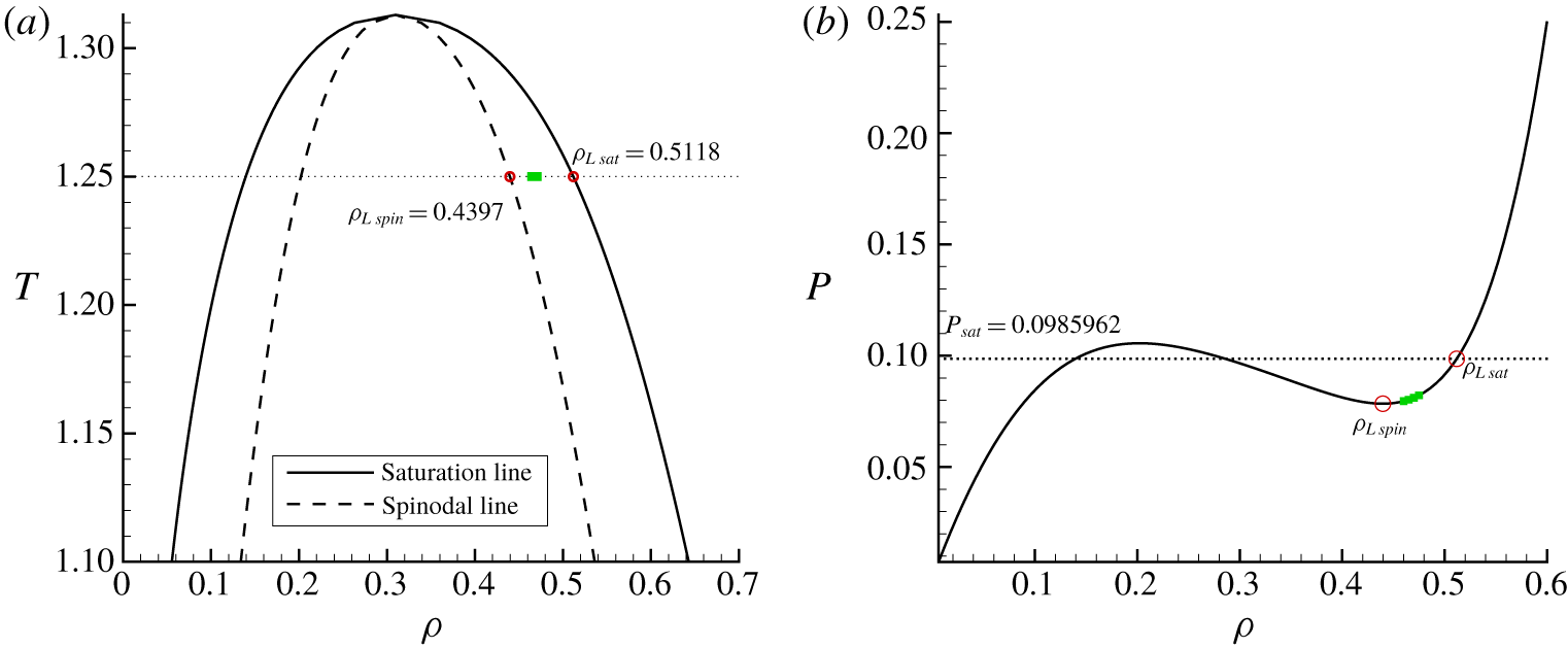
(a) Phase diagram of a Lennard Jones fluid described with the modified Benedict–Webb–Rubin equation of state. The solid line represents the saturation conditions, corresponding to the vapour and liquid densities at equilibrium. The dashed curve represents the spinodal line, where the condition  $\unicode[STIX]{x2202}p/\unicode[STIX]{x2202}\unicode[STIX]{x1D70C}|_{T}=0$ is satisfied. (b) The isotherm
 $T=1.25$ in the
 $P$–
 $\unicode[STIX]{x1D70C}$ plane. The dotted line represents the saturation pressure. In both panels the green symbols corresponds to the metastable conditions investigated with the spherical FH simulations.

The energy landscape obtained with the string method is here compared with the one provided by the CNT
 $$\begin{eqnarray}\unicode[STIX]{x0394}\unicode[STIX]{x1D6FA}^{CNT}(R)=\unicode[STIX]{x0394}p{\textstyle \frac{4}{3}}\unicode[STIX]{x03C0}R^{3}+\unicode[STIX]{x1D6FE}4\unicode[STIX]{x03C0}R^{2},\end{eqnarray}$$
where  $\unicode[STIX]{x0394}p$ is the pressure difference between liquid and vapour and
 $\unicode[STIX]{x1D6FE}$ the surface tension.
The phase diagram for the modified MBWR EoS is given in figure 1(a) where both the spinodal line (dashed) and the saturation line (solid) are plotted as a function of the temperature. The region between the liquid branches of the spinodal and saturation lines corresponds to metastable liquid states. All the thermodynamic conditions analysed in this work have been chosen at a temperature of  $T=1.25$, where the metastable region spans in the liquid density range
 $\unicode[STIX]{x1D70C}_{Lspin}=0.4397<\unicode[STIX]{x1D70C}_{L}^{met}<\unicode[STIX]{x1D70C}_{Lsat}=0.5118$ (both temperature and densities are expressed in LJ units, see below).
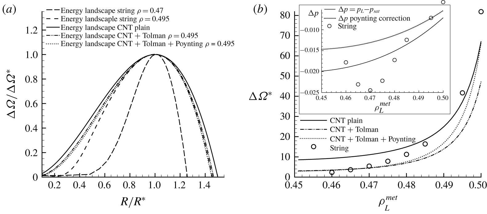
(a) Free energy landscape (normalized with the energy barrier  $\unicode[STIX]{x0394}\unicode[STIX]{x1D6FA}^{\ast }$) as a function of the bubble radius (normalized with the critical radius
 $R^{\ast }$). The solid line corresponds to the CNT prediction, while the other two curves have been obtained with the string method at two different metastable liquid densities, both at
 $T=1.25$. (b) Comparison of the energy barriers between different CNT models and the string results. The ‘
 $\text{CNT}+\text{Tolman}$’ corresponds to the proposed correction by Menzl et al. (Reference Menzl, Gonzalez, Geiger, Caupin, Abascal, Valeriani and Dellago2016) with an optimal fitting Tolman length
 $\unicode[STIX]{x1D6FF}=0.964$. The ‘
 $\text{CNT}+\text{Tolman}+\text{Poynting}$’ adds the Poynting correction to the pressure difference (plotted in the inset) as suggested by Angélil et al. (Reference Angélil, Diemand, Tanaka and Tanaka2014) with an optimal fitting Tolman length
 $\unicode[STIX]{x1D6FF}=1.95$.

In figure 2(a) we compare the landscapes of three different CNT predictions with those obtained with the string method at two specific thermodynamic conditions:  $\{\unicode[STIX]{x1D70C}_{L}^{met}=0.47,T=1.25\}$ and
 $\{\unicode[STIX]{x1D70C}_{L}^{met}=0.495,T=1.25\}$. The condition with the higher density is closer to saturation (
 $\unicode[STIX]{x1D70C}_{Lsat}=0.5118$), where the CNT is expected to provide accurate results. Indeed, near saturation, the critical bubble is larger and the density distribution is better approximated as a sharp profile (interface thickness much smaller than the bubble radius), consistently with the CNT hypothesis. In the ‘plain CNT’ model (solid line) the surface tension is assumed constant,
 $\unicode[STIX]{x1D6FE}=0.059$ as appropriate for an LJ fluid at
 $T=1.25$, and the pressure difference is given by
 $\unicode[STIX]{x0394}p=p_{L}-p_{sat}$. In the two chosen metastable states
 $\unicode[STIX]{x0394}p=-0.01749$ and
 $\unicode[STIX]{x0394}p=-0.00958$, respectively. The ‘
 $\text{CNT}+\text{Tolman}$’ (dash–double-dotted line) model introduces the Tolman length correction for the surface tension,
 $\unicode[STIX]{x1D6FE}=\unicode[STIX]{x1D6FE}_{0}/(1+2\unicode[STIX]{x1D6FF}/R)$, as suggested by Menzl et al. (Reference Menzl, Gonzalez, Geiger, Caupin, Abascal, Valeriani and Dellago2016). The ‘
 $\text{CNT}+\text{Tolman}+\text{Poynting}$’ (dotted line) model adds the Poynting correction to the pressure difference which takes into account the fact that the vapour is not at the saturation pressure (Blander & Katz Reference Blander and Katz1975), as exploited by Angélil et al. (Reference Angélil, Diemand, Tanaka and Tanaka2014). The Tolman length,
 $\unicode[STIX]{x1D6FF}$, is used as a free parameter to fit the energy barriers over those provided by the string method, figure 2(b). The optimal values are
 $\unicode[STIX]{x1D6FF}=0.964$ and
 $\unicode[STIX]{x1D6FF}=1.95$, respectively. The values obtained from the present data are a bit large when compared to other works in the literature, see for instance Menzl et al. (Reference Menzl, Gonzalez, Geiger, Caupin, Abascal, Valeriani and Dellago2016). However, it should be noted that our simulations are performed close to the critical point and that the Tolman length is an increasing function of temperature. It is worth noticing that the Tolman correction helps in reducing the barrier errors in the region of lower densities, closer to the spinodal condition, where the critical radius is expected to be smaller. On the other hand, the Poynting correction helps to recover a good level of approximation also in the intermediate metastability region. As apparent in the inset of figure 2(b), the pressure difference correction obtained with the Poynting model allows us to perfectly reproduce the values for
 $\unicode[STIX]{x1D70C}_{L}^{met}>0.49$ obtained with the string method. Within the string method,
 $\unicode[STIX]{x0394}p$ is evaluated as the pressure difference between the liquid and the bubble centre,
 $\unicode[STIX]{x0394}p=p_{L}-p_{V}=p(\unicode[STIX]{x1D70C}_{L}^{met})-p(\unicode[STIX]{x1D70C}(r=0))$. When approaching the spinodal condition,
 $\unicode[STIX]{x1D70C}_{L}^{met}\rightarrow \unicode[STIX]{x1D70C}_{Lspin}$, the density profiles become flatter and the density at the bubble centre increases,
 $\unicode[STIX]{x1D70C}(r=0)\rightarrow \unicode[STIX]{x1D70C}_{L}^{met}$. As a consequence, the magnitude of the pressure difference is reduced and tends to vanish,
 $\unicode[STIX]{x0394}p\rightarrow 0$, explaining the non-trivial behaviour observed in figure 2(b). Please note that this effect, not captured by any CNT approach, was also observed in Shen & Debenedetti (Reference Shen and Debenedetti2001), who exploited the density functional theory to study the free energy landscapes of vapour bubble nucleation. Figure 2(a) shows that, as expected, the closer the condition is to the saturation point, the better is the CNT approximation in comparison with the more detailed description of the diffuse interface modelling. The two corrections added to the plain CNT model allow us to reduce the error, in particular when the bubble is larger than the critical one.
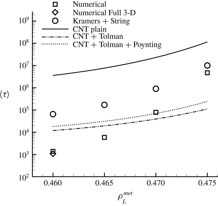
The MEP gives access to the mean first passage time  $\langle \unicode[STIX]{x1D70F}\rangle$ through the well-established Kramers theory (Kramers Reference Kramers1940). In a nutshell, the theory assumes that the probability of observing a vapour cluster with radius
 $R$ is proportional to
 $\exp (-\unicode[STIX]{x0394}\unicode[STIX]{x1D6FA}(R)/\text{k}_{B}T)$ and that the system spends most of the time close to the metastable condition. The escape dynamics from the metastable basin follows a diffusive motion, hence the mean passage time can be approximated by evaluating the integral,
 $$\begin{eqnarray}\langle \unicode[STIX]{x1D70F}\rangle =\int _{\cup }\exp \left(-\frac{\unicode[STIX]{x0394}\unicode[STIX]{x1D6FA}(R)}{\text{k}_{B}T}\right)\,\text{d}R\int _{\cap }\frac{1}{D}\exp \left(\frac{\unicode[STIX]{x0394}\unicode[STIX]{x1D6FA}(R)}{\text{k}_{B}T}\right)\,\text{d}R,\end{eqnarray}$$
where  $\cup$ and
 $\cap$ represent the metastable and the critical basin, respectively (see appendix B for details). In (2.38) the parameter
 $D$ is the diffusion coefficient here evaluated, following Menzl et al. (Reference Menzl, Gonzalez, Geiger, Caupin, Abascal, Valeriani and Dellago2016), as
 $D^{\ast }=\text{k}_{B}T/16\unicode[STIX]{x1D702}\unicode[STIX]{x03C0}R^{\ast }$ estimated at the critical state. It is obtained by enforcing the fluctuation dissipation balance on the stochastic over-damped Rayleigh–Plesset dynamics for the bubble radius. It is thus clear that the most relevant aspects in the energy landscape in figure 2(a) are the basin regions and, in particular, its curvatures in the metastable condition (
 $R\simeq 0$) and at the transition point (
 $R\simeq R^{\ast }$). The results show that the finite thickness of the vapour–liquid interface at the thermodynamic condition closer to saturation does not strongly affect the energy landscape at the transition state. This is in line with the expected behaviour, consistently with the CNT hypothesis. On the contrary, at smaller radii, where the vapour cluster dimension is comparable with its interface thickness, the curvatures obtained with the string method in both the thermodynamic conditions analysed are substantially different from those following from CNT. This discrepancy highlights the importance of considering a phase field description when dealing with phase transitions.
3 Results and discussion
3.1 Equation of state
As already stated, also for the stochastic simulations the selected bulk free energy  $f_{b}(\unicode[STIX]{x1D70C},T)$ is the modified Benedict–Webb–Rubin equation of state (Johnson et al. Reference Johnson, Zollweg and Gubbins1993). All quantities are made dimensionless by introducing as reference values the parameters of the LJ potential:
 $\unicode[STIX]{x1D70E}=3.4\times 10^{-10}~\text{m}$ as length,
 $\unicode[STIX]{x1D716}=1.65\times 10^{-21}~\text{J}$ as energy,
 $m=6.63\times 10^{-26}~\text{kg}$ as mass and
 $T_{r}=\unicode[STIX]{x1D716}/\text{k}_{B}$ as temperature. In order to reproduce the benchmark results for surface tension obtained through Monte Carlo simulations, the capillary coefficient is fixed as
 $\unicode[STIX]{x1D706}=\unicode[STIX]{x1D706}m^{2}/(\unicode[STIX]{x1D70E}^{5}\unicode[STIX]{x1D716})=5.224$ (Gallo et al. Reference Gallo, Magaletti and Casciola2018b). It is worth noticing that, in the present diffuse interface model,
 $f_{b}(\unicode[STIX]{x1D70C},T)$ and
 $\unicode[STIX]{x1D706}$ determine both surface tension and interface thickness on physical grounds, see Magaletti et al. (Reference Magaletti, Gallo, Marino and Casciola2016) for details. In particular, the interface thickness is
 $$\begin{eqnarray}\unicode[STIX]{x1D716}=(\unicode[STIX]{x1D70C}_{L}-\unicode[STIX]{x1D70C}_{V})\sqrt{\frac{\unicode[STIX]{x1D706}}{2[w_{b}(\bar{\unicode[STIX]{x1D70C}})-w_{b}(\unicode[STIX]{x1D70C}_{V})]}},\end{eqnarray}$$
where  $w_{b}$ is the Landau grand potential density
 $w_{b}=f_{b}-\unicode[STIX]{x1D707}_{eq}\unicode[STIX]{x1D70C}$,
 $\unicode[STIX]{x1D707}_{eq}$ being the equilibrium chemical potential at saturation,
 $\unicode[STIX]{x1D70C}_{L}$ and
 $\unicode[STIX]{x1D70C}_{V}$ the density values of liquid and vapour at saturation and
 $\bar{\unicode[STIX]{x1D70C}}$ the density corresponding to the condition
 $\unicode[STIX]{x2202}w_{b}/\unicode[STIX]{x2202}\unicode[STIX]{x1D70C}=0$. Similarly, the surface tension follows as
 $$\begin{eqnarray}\unicode[STIX]{x1D6FE}=\int _{\unicode[STIX]{x1D70C}_{V}}^{\unicode[STIX]{x1D70C}_{L}}\sqrt{2\unicode[STIX]{x1D706}(w_{b}(\unicode[STIX]{x1D70C})-w_{b}(\unicode[STIX]{x1D70C}_{V}))}\,\text{d}\unicode[STIX]{x1D70C}.\end{eqnarray}$$
With the chosen  $f_{b}$ and
 $\unicode[STIX]{x1D706}$ the dimensionless (LJ units) surface tension and interface thickness are
 $\unicode[STIX]{x1D6FE}=0.059$ and
 $\unicode[STIX]{x1D716}=8.46$, respectively, which correspond to
 $\unicode[STIX]{x1D6FE}=8.42\times 10^{-4}~\text{J}~\text{m}^{-2}$ and
 $\unicode[STIX]{x1D716}=2.86\times 10^{-9}~\text{m}$, when using argon parameters. One LJ time unit would correspond to
 $2.15\times 10^{-12}~\text{s}$, with a reference density of
 $1.69\times 10^{3}~\text{kg}~\text{m}^{-3}$. Clearly, the approach is not limited to argon, which is the prototypal system for validation against molecular dynamics simulations. Other fluids can be used, e.g. water, by selecting the appropriate free energy equation and capillary coefficient.
In order to be fully consistent with the LJ properties, the expression proposed by Rowley & Painter (Reference Rowley and Painter1997) for viscosity  $\unicode[STIX]{x1D702}(\unicode[STIX]{x1D70C},T)$ is used. This choice enables us to account for the substantial viscosity change between the liquid and vapour phase.
3.2 Numerical scheme and the discrete fluctuation dissipation balance
The different physical phenomena captured by (2.29)–(2.30) make their numerical treatment challenging. Specifically, both the stochastic contribution and the deterministic part, characterized by phase change, acoustic wave emission, capillary dispersion and viscous diffusion, call for specialized numerical techniques. In our previous works (Magaletti et al. Reference Magaletti, Marino and Casciola2015, Reference Magaletti, Gallo, Marino and Casciola2016) a staggered scheme coupled with an explicit Runge–Kutta integrator has been employed to numerically solve the deterministic diffuse interface equations. When dealing with stochastic partial differential equations, dissipative numerical schemes should always be avoided since they introduce artificial dissipation that would spoil the fluctuation–dissipation balance. In order to comply with this requirement, we adopt a classical centred second-order approximation on a uniform, staggered grid where scalars are located at the cell centres, while (radial) vectors are located at the cell boundaries, as described in Balboa et al. (Reference Balboa, Bell, Delgado-Buscalioni, Donev, Fai, Griffith and Peskin2012). This scheme inherits at discrete level the required functional properties of the continuum differential operators (skew adjointness of the gradient,  $\unicode[STIX]{x1D735}\boldsymbol{\cdot }=-\unicode[STIX]{x1D735}^{\dagger }$, and self-adjointness of the Laplacian,
 $(\unicode[STIX]{x1D6FB}^{2})^{\dagger }=(\unicode[STIX]{x1D735})^{\dagger }\boldsymbol{\cdot }(\unicode[STIX]{x1D735}\boldsymbol{\cdot })^{\dagger }=\unicode[STIX]{x1D6FB}^{2}$ (Balboa et al. Reference Balboa, Bell, Delgado-Buscalioni, Donev, Fai, Griffith and Peskin2012)). Concerning time integration, the use of specific explicit Runge–Kutta schemes is advised when dealing with stochastic equations (Honeycutt Reference Honeycutt1992). In particular, here a second-order accurate stochastic Runge–Kutta integrator is used. The adopted numerical method satisfies at discrete level the fluctuation–dissipation balance, i.e. the scheme reproduces the theoretical equilibrium covariances of the fluctuating fields. In particular, concerning stochastic fluxes, it is second-order accurate in time in a weak sense, and it recovers also the second-order (strong) accuracy for the deterministic part of the equations.
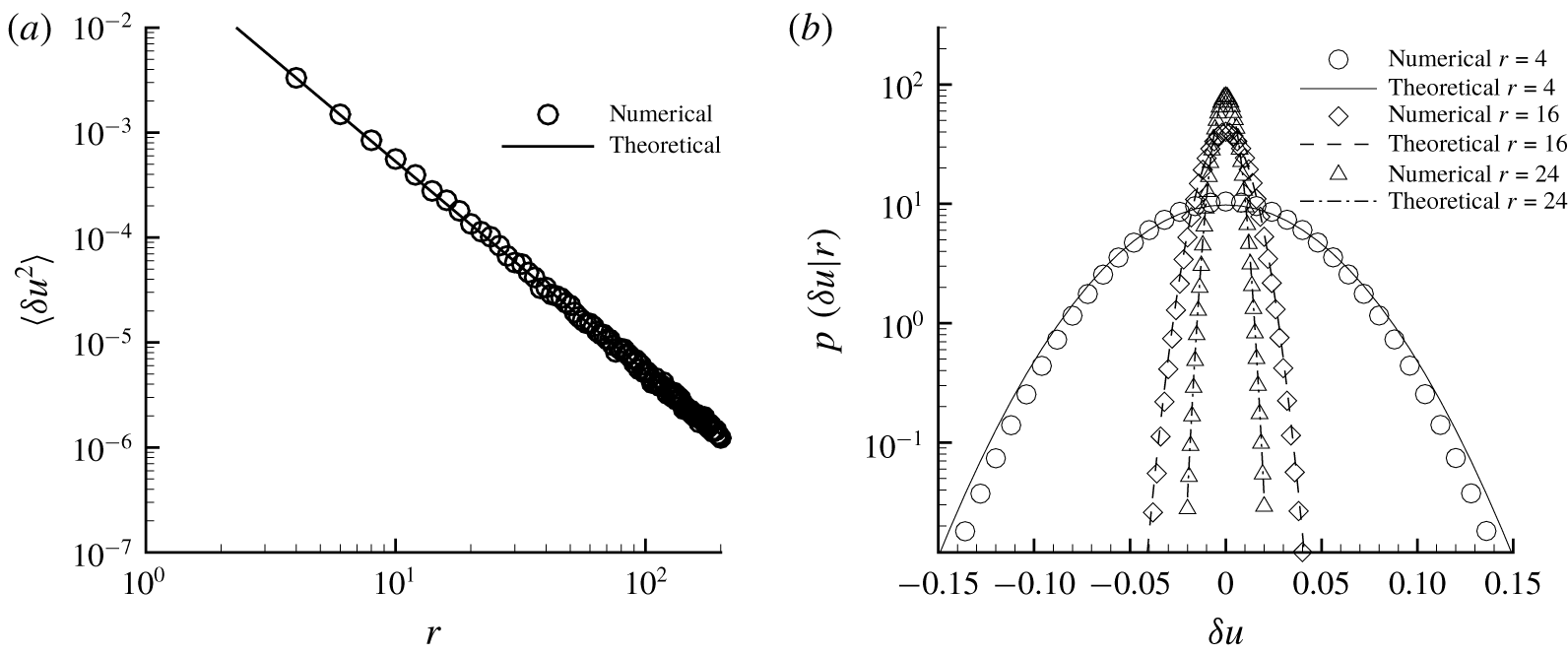
As common in the specific literature (Donev et al. Reference Donev, Vanden-Eijnden, Garcia and Bell2010; Balboa et al. Reference Balboa, Bell, Delgado-Buscalioni, Donev, Fai, Griffith and Peskin2012; Delong et al. Reference Delong, Griffith, Vanden-Eijnden and Donev2013) the convergence of the adopted numerical scheme is validated by comparing the statistical properties of the radial velocity field with their theoretical predictions. Clearly, when dealing with stochastic systems, all that concerns convergence must be checked on statistical properties, a single realization alone bearing no physical significance. The expected variance of spherically symmetric velocity fluctuations can be obtained from the general Cartesian expression (2.10) as
 $$\begin{eqnarray}\langle \unicode[STIX]{x1D6FF}u(r)\unicode[STIX]{x1D6FF}u(r)\rangle =\frac{\text{k}_{B}T_{0}}{4\unicode[STIX]{x03C0}\unicode[STIX]{x1D70C}_{0}\unicode[STIX]{x0394}r}r^{-2},\end{eqnarray}$$
with  $\unicode[STIX]{x1D70C}_{0}$ the mean density,
 $\unicode[STIX]{x0394}r$ the grid size and
 $T_{0}$ the temperature. The comparison is provided in figure 3(a) showing a perfect agreement and confirming that the discrete FDB is perfectly satisfied by the numerical scheme. The probability density function of velocity fluctuations at different radial positions are shown in figure 3(b), as a further common accuracy check used in the fluctuating hydrodynamics community (Voulgarakis & Chu Reference Voulgarakis and Chu2009; Lazaridis, Wickham & Voulgarakis Reference Lazaridis, Wickham and Voulgarakis2017).
(a) Velocity fluctuation variance versus radial coordinate  $r$ (theoretical prediction, solid line; numerical results, symbols). (b) Probability density function of velocity fluctuations at three different radial coordinates (theoretical predictions, solid line; numerical results, symbols).

3.3 Vapour bubble nucleation
Bubble nucleation is investigated in a metastable liquid enclosed in a spherical domain with radius  $R_{wall}=200$ with fixed temperature, volume and total mass (NVT ensemble). For the sake of definiteness, the spherical solid wall is assumed to enforce impermeability and a no-slip condition with vanishing density normal derivative. The related wettability would correspond to a
 $90^{\circ }$ contact angle. In fact, the impermeability condition induces confinement effects on the dynamics that, for small systems, may be significant and will be described in § 3.4, devoted to bubble oscillations. On the contrary, the wettability is selected to prevent fluid layering at the wall, an effect estimated to be negligible for the present systems since it takes place far from the bubble, within an extremely thin wall layer. The system has been spatially discretized on a uniform grid with
 $50$ cells, corresponding to a dimensional cell length
 $\unicode[STIX]{x0394}r=1.36~\text{nm}$. As reported in § 3.1, the nominal interface thickness is
 $\unicode[STIX]{x1D716}=2.86~\text{nm}$, hence the used grid guarantees a good spatial accuracy with 8–10 cells inside the interface, since its actual thickness is 4–5 times
 $\unicode[STIX]{x1D716}$ (Jacqmin Reference Jacqmin1999). As initial condition we use a quiescent fluid at different homogeneous metastable liquid density
 $\unicode[STIX]{x1D70C}_{L}^{met}$. The different conditions are highlighted with green symbols in the phase diagram of figure 1(a). Twenty simulations for each thermodynamic condition were run using different seeds for the random number generator used for the Gaussian noise. Convergence tests assured that the number of samples is sufficient for statistical accuracy (error within 3 %–4 %).
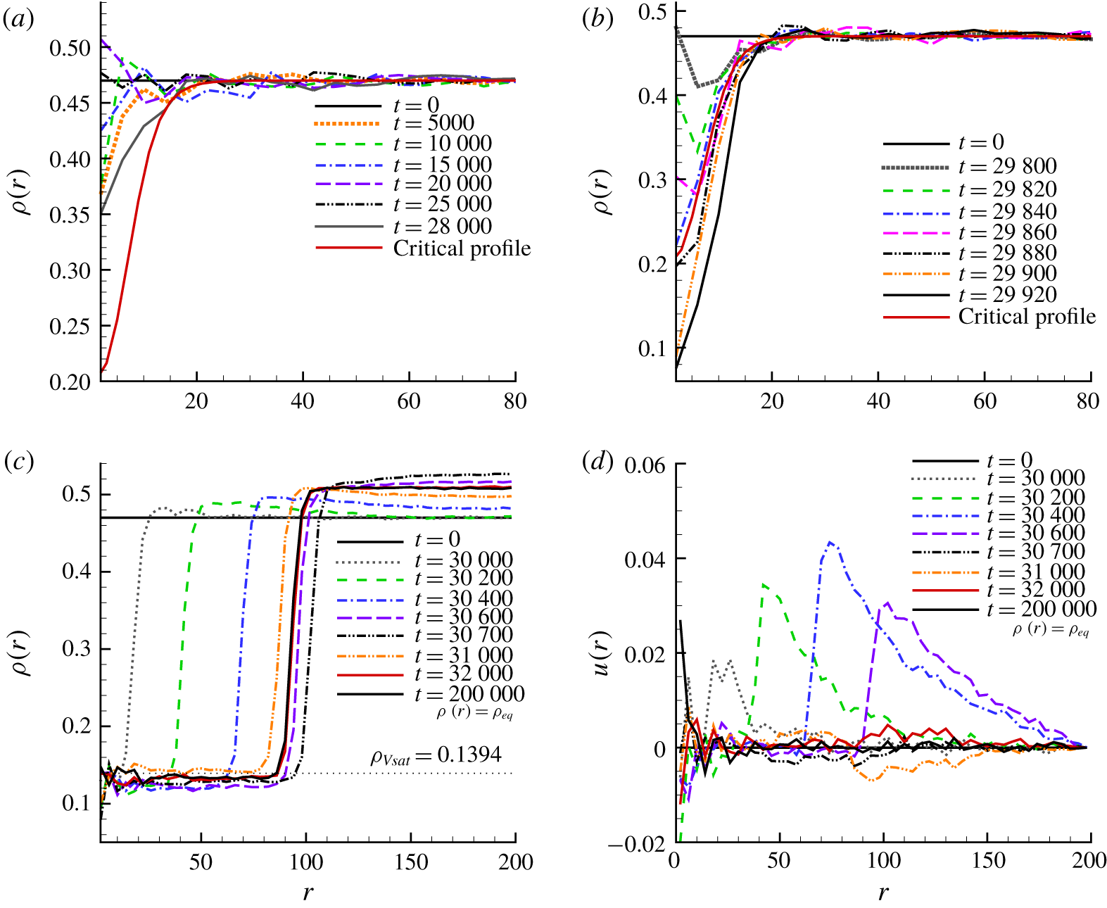
Density and velocity evolution in a closed system with  $R_{wall}=200$ at
 $\unicode[STIX]{x1D70C}_{L}^{met}=0.46$. (a) Density profiles versus radial distance
 $r$ at different time instants before the nucleation event. The critical profile (red solid line), evaluated with the string method, is reported as a reference. (b) Density profiles during the critical bubble formation. (c) Density profiles during the inertial growth and oscillation stage. (d) Radial velocity profiles during the inertial growth and oscillation stage.

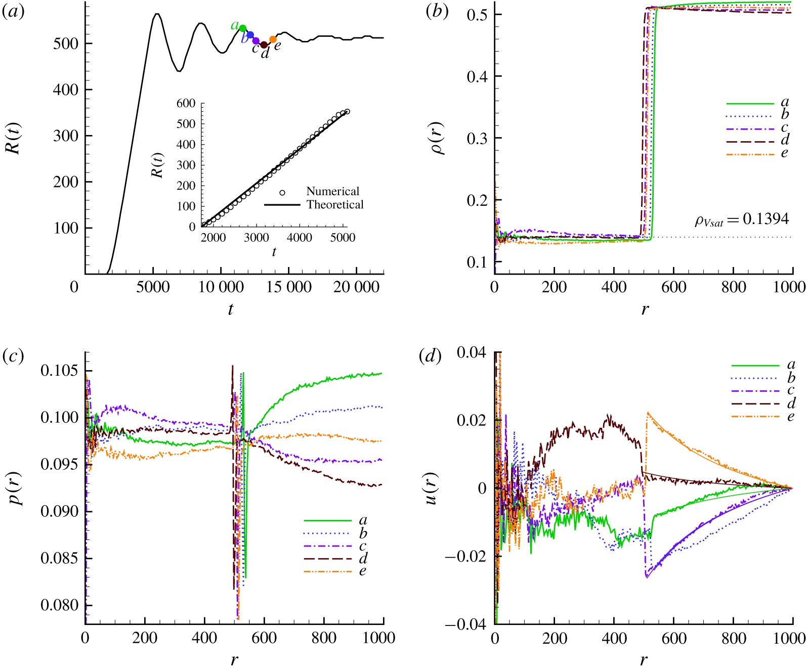
System (2.29)–(2.31) is integrated until it reaches the stable state with a mature, larger than critical, vapour bubble surrounded by the liquid compressed to density larger than the initial metastable one,  $\unicode[STIX]{x1D70C}_{L}^{met}$. The density and velocity radial profiles are plotted in figure 4 at different time instants. The figure refers to one configuration randomly extracted from the twenty different simulations; radial profiles and transition times do differ for each sample but the qualitative dynamics is substantially the same. Each panel focuses on one evolution stage among (a) pre-nucleation, (b) critical bubble formation, (c) inertial growth and oscillation dynamics. Panel (d) concerns the velocity profiles during the growth regime. In both figures 4(a) and 4(b) the critical cluster density profile obtained with the string method is plotted as reference (red solid line). Figure 4(a) shows density variations developing from the initial homogeneous liquid phase due to thermal fluctuations. They are particularly intense in the proximity of the cluster centre, near
 $r=0$, where the density correlation is expected to be higher from theory. During this first evolution stage the system explores the metastable basin: most of the time the configuration consists of a cluster smaller than the critical one but, on rare occasions, the cluster grows to larger sizes (comparable to critical) retaining however a density significantly larger than will be found in the critical bubble (solid grey line). Sometimes the density in the cluster core may even exceed that of the metastable liquid (see, e.g. the dashed purple line). Such configurations (
 $\unicode[STIX]{x1D70C}(r=0)>\unicode[STIX]{x1D70C}_{L}^{met}$) are always suppressed given the limited compressibility of the high density fluid which entails a large pressure increase. These observations suggest that the classical description of the phase transition with a single order parameter, namely the bubble radius, could miss important details. From inspection, nucleation events are most often initiated by an intense density fluctuation near the nucleus centre which allows the system to cross the transition barrier. When this occurs, the dynamics is extremely fast; see the range of times involved in figure 4(b). As soon as the vapour cluster becomes larger than the critical size and its density becomes sufficiently low, the bubble suddenly expands to reaches the equilibrium size on a time scale (order of
 $10^{3}$ time units) much smaller than the time required to activate the transition (order of
 $10^{4}$ time units for this thermodynamic condition). The density and the radial velocity profiles during this inertial growth stage are plotted in figures 4(c) and 4(d), respectively. During the growth phase the vapour density remains almost constant, slightly lower than the saturation level (
 $\unicode[STIX]{x1D70C}_{Vsat}=0.1394$). Meanwhile, liquid pressure and density increase. During the oscillation the vapour is slightly compressed (orange dash–double-dotted line), but re-expands back until the equilibrium is reached. Figure 4(d) shows that the velocity inside the bubble during inertial growth is dominated by the noise and is almost negligible with respect to the bubble interface velocity and, consequently, with respect to the velocity of the exterior liquid.
The ensemble of simulations with different random seeds allows us to evaluate the mean first passage time  $\langle \unicode[STIX]{x1D70F}\rangle$. From an operative point of view, the transition time of a single simulation is identified as the time when the bubble starts growing explosively. As discussed in the context of density profile analysis, the expansion stage is so fast that any possible indetermination in evaluating the actual transition time is comparatively negligible. The mean first passage time obtained from the spherical model, figure 5, can be compared with the results of full 3-D FH simulations. The computational cost of the full model suggests we restrict the comparison to a single thermodynamic condition sufficiently close to the spinodal point,
 $\unicode[STIX]{x1D70C}_{L}^{met}=0.46$. It may be stressed that, theoretically, this is the most challenging case, since far from the spinodal CNT already provides a good reference. In order to reduce the effects of the multi-bubble nucleation observed with the full 3-D simulations we reduced the 3-D domain to a
 $160\times 160\times 160$ box, obtaining the formation of a single (or very few) bubble at a time. The evaluated mean first passage time compares extremely well with the full 3-D simulation, confirming the effectiveness of the spherical model assumptions exploited in § 2.3 and the possibility of neglecting angular terms. The numerical results are also compared with the theoretical prediction of Kramers theory applied to both the string method, as explained in § 2.4, and to the CNT energy landscapes plotted in figure 2(a). The plain CNT predictions are by far the worst, in particular close to spinodal conditions. The other two CNT approaches with Tolman and Poynting corrections better approximate the mean first passage time. This is motivated by the fact that the Tolman length was determined by fitting from the string method (§ 2.4) the free energy barrier which is the crucial parameter determining the mean first passage time. The comparison with the ‘
 $\text{Kramers}+\text{String}$’ approach clearly shows the expected trend, with the numerical simulation approaching the theoretical prediction at higher densities, hence at smaller metastability level. It is indeed expected (see appendix B) that the Kramers approximation for the mean first passage time becomes valid when the energy barriers are high. As a consequence, the closer to saturation the thermodynamic condition is, the more accurate becomes Kramers theory.
Mean first passage time at different thermodynamic conditions. The squares represent the numerical calculation with the spherically reduced model and the circles the prediction with Kramers theory coupled with the string method. The diamond symbol corresponds to a full 3-D simulation with the FH model. The curves are obtained by applying Kramers theory to the different CNT energy landscapes plotted in figure 2(a).

3.4 Bubble dynamics
One of the main features of the present model is the possibility of accessing the full nucleation process, from the phase change inception up to the macroscopic hydrodynamic motion, all within the same framework. From a computational standpoint, the present approach is much cheaper than both atomistic simulations (Diemand et al. Reference Diemand, Angélil, Tanaka and Tanaka2013) and full 3-D fluctuating hydrodynamic theory (Gallo, Magaletti & Casciola Reference Gallo, Magaletti and Casciola2018a; Gallo et al. Reference Gallo, Magaletti and Casciola2018b), facilitating the analysis of the complete dynamics. In particular the numerical effort required by an atomistic simulation, see e.g. Diemand et al. (Reference Diemand, Angélil, Tanaka and Tanaka2013), LAMMPS LJ benchmarks, is of the order of  $4\times 10^{4}$ core hours to follow nucleation in a
 $(300~\text{nm})^{3}$ system for
 $1~\text{ns}$, enabling the evaluation of the nucleation rate. A full three-dimensional FH simulation in a thermodynamic condition with a comparable nucleation rate and an equivalent domain size requires of order
 $10^{2}$ core hours to capture the complete nucleation regime. At the same condition, the present model requires only
 $1$ core hour to simulate a time corresponding to twice the mean first passage time, hence observing the bubble formation event with a four orders of magnitude cheaper simulation with respect to brute-force molecular dynamics (MD).
Inertial growth and oscillation stage in a closed system with  $R_{wall}=1000$ at
 $\unicode[STIX]{x1D70C}_{L}^{met}=0.46$. (a) Bubble radius evolution. In the inset the expansion stage is compared with Rayleigh’s prediction. The labels denote the time of the five snapshots shown in the other panels. (b) Density profiles during the oscillation. The dotted line provides the vapour saturation density. (c) Pressure profiles. (d) Velocity profiles compared with Vincent & Marmottant (Reference Vincent and Marmottant2017) plotted as solid lines; the solid blue and purple curves (b,c lines) happened to be almost coincident, while an intense stochastic fluctuation in the particular configuration shown with the dotted (b) curve produced a deviation from the expected trend.

In this section we focus on the cavitation dynamics in a large confined medium. This problem has attracted great attention from researchers (Vincent et al. Reference Vincent, Marmottant, Quinto-Su and Ohl2012, Reference Vincent, Marmottant, Gonzalez-Avila, Ando and Ohl2014; Drysdale et al. Reference Drysdale, Doinikov and Marmottant2017; Vincent & Marmottant Reference Vincent and Marmottant2017; Scognamiglio et al. Reference Scognamiglio, Magaletti, Izmaylov, Gallo, Casciola and Noblin2018) since several similar scenarios occur in nature, e.g. the cavitation process in tree xylems. The system we study consists again of a wall bounded sphere, now with radius  $R=1000$, much larger than for the cases discussed in the previous section. The grid size is kept identical,
 $\unicode[STIX]{x0394}r=4$, since the resolution is dictated by the interface thickness. As before, the system is initialized in a homogeneous metastable liquid state and, after a time of the order of the mean first passage time, the thermal noise activates the nucleation process. When the bubble appears the dynamics can be divided into two different phases, as shown in figure 6(a). In the first stage the bubble expands at (almost) constant velocity until reaching its maximum radius. After that, due to the total mass constraint, the bubble starts oscillating. This second stage is characterized by a damped oscillation at a specific frequency, until relaxation to the equilibrium state. The expansion at constant growth rate follows the prediction of the classical Rayleigh–Plesset model (Brennen Reference Brennen2013)
 $$\begin{eqnarray}{\dot{R}}=\sqrt{\frac{2}{3}\,\frac{p_{sat}-p_{L}^{met}}{\unicode[STIX]{x1D70C}_{L}^{met}}},\end{eqnarray}$$
where  $p_{sat}$ is the saturation pressure and
 $p_{L}^{met}$ the pressure in the metastable liquid at the initial condition. The comparison between the simulation and the theoretical prediction is shown in the inset of figure 6(a). In this regime, the bubble growth is mainly driven by the pressure difference between vapour (roughly at saturation conditions) and the liquid held at constant pressure far away from the bubble interface. This linear growth regime has been also observed in large MD simulations of bubble nucleation (Angélil et al. Reference Angélil, Diemand, Tanaka and Tanaka2014).
Concerning the second stage, density, pressure and velocity profiles are shown in figures 6(b), 6(c) and 6(d), respectively. The third oscillation, after the strong transient and the nonlinearities associated with the initial explosive growth are damped away, can be selected for fair comparison with existing theoretical models for bubble oscillations. From figure 6(b) it is apparent that the liquid density is almost homogeneous in space, and varies in time according to the bubble oscillation. The spatial variation is smaller than 2 %, showing that the quasi-static approximation proposed by Vincent & Marmottant (Reference Vincent and Marmottant2017) is quite accurate. The small variation in density is reflected in a slightly larger variation in pressure, which still remains below 5 %, as shown in figure 6(c). The strong pressure gradient is concentrated inside the narrow interface and associated with the capillary stress, as clearly visible in the profiles.
In order to compare the present results with the model proposed by Vincent & Marmottant (Reference Vincent and Marmottant2017), a slightly extended version of their theory is advisable to cope with the high temperature thermodynamic conditions involved here. The original theory neglected the vapour density since in most common conditions  $\unicode[STIX]{x1D70C}_{V}/\unicode[STIX]{x1D70C}_{L}\ll 1$. This is not the case at higher temperature. In particular, at
 $T=1.25$, the saturation densities for vapour and liquid are
 $\unicode[STIX]{x1D70C}_{Vsat}=0.1394$ and
 $\unicode[STIX]{x1D70C}_{Lsat}=0.5118$, respectively. For a confined system, mass conservation implies a relation between bubble radius and the liquid density,
 $$\begin{eqnarray}\unicode[STIX]{x1D70C}_{L}(R_{wall}^{3}-R^{3})+\unicode[STIX]{x1D70C}_{V}R^{3}=\unicode[STIX]{x1D70C}_{L}^{met}R_{wall}^{3}.\end{eqnarray}$$
Assuming vapour density at saturation,  $\unicode[STIX]{x1D70C}_{V}=\unicode[STIX]{x1D70C}_{Vsat}$, as reasonable according to figure 6(b), the liquid density reads
 $$\begin{eqnarray}\unicode[STIX]{x1D70C}_{L}=\frac{\unicode[STIX]{x1D70C}_{L}^{met}-\unicode[STIX]{x1D70C}_{Vsat}x^{3}}{1-x^{3}},\end{eqnarray}$$
with  $x=R/R_{wall}$. Under the assumption of quasi-static evolution, as in Vincent & Marmottant (Reference Vincent and Marmottant2017), the liquid density is spatially homogeneous, entailing, by mass conservation, a simple relation between liquid velocity, liquid density and interface velocity
 ${\dot{R}}$,
 $$\begin{eqnarray}\unicode[STIX]{x1D735}\boldsymbol{\cdot }\boldsymbol{u}=\frac{1}{r^{2}}\frac{\unicode[STIX]{x2202}(r^{2}u)}{\unicode[STIX]{x2202}r}=-\frac{\dot{\unicode[STIX]{x1D70C}_{L}}}{\unicode[STIX]{x1D70C}_{L}}.\end{eqnarray}$$
By exploiting the boundary condition,  $u(R_{wall})=0$ at the confining wall, integration leads to
 $$\begin{eqnarray}u(r)=\frac{(\unicode[STIX]{x1D70C}_{L}^{met}-\unicode[STIX]{x1D70C}_{Vsat})}{(\unicode[STIX]{x1D70C}_{L}^{met}-x^{3}\unicode[STIX]{x1D70C}_{Vsat})}\frac{x^{2}}{(1-x^{3})}{\dot{R}}\left[\frac{R_{wall}^{2}}{r^{2}}-\frac{r}{R_{wall}}\right]\,.\end{eqnarray}$$
Figure 6(d) shows the good agreement between the numerical velocity profiles and this theoretical prediction.
The bubble frequency  $f$ is easily extracted from the numerical simulations and compared with two theoretical predictions: (i) the Drysdale et al. (Reference Drysdale, Doinikov and Marmottant2017) prediction, based on the following equation in terms of the complex oscillation pulsation,
 $\unicode[STIX]{x1D714}$ (
 $f=Re[\unicode[STIX]{x1D714}]/(2\unicode[STIX]{x03C0})$):
 $$\begin{eqnarray}1-kR_{wall}\frac{1+2\text{i}\unicode[STIX]{x1D709}_{b}^{2}(1-R_{eq}/R_{wall})}{\tan [k(R_{wall}-R_{eq})]}+2\text{i}\unicode[STIX]{x1D709}_{b}^{2}(1+k^{2}R_{eq}R_{wall})=0,\end{eqnarray}$$
with  $R_{eq}$ the final equilibrium bubble radius in the confined system,
 $\unicode[STIX]{x1D709}_{b}=\unicode[STIX]{x1D6FF}/R_{eq}$,
 $\unicode[STIX]{x1D6FF}=(2\unicode[STIX]{x1D702}/(\unicode[STIX]{x1D714}\unicode[STIX]{x1D70C}_{Leq}))^{1/2}$,
 $\unicode[STIX]{x1D702}$ the fluid viscosity,
 $\unicode[STIX]{x1D70C}_{Leq}$ the liquid density at equilibrium obtained with (3.6),
 $k=\unicode[STIX]{x1D714}/(c_{eq}(1-\text{i}4/3\unicode[STIX]{x1D702}\unicode[STIX]{x1D714}/(\unicode[STIX]{x1D70C}_{Leq}c_{eq}^{2}))^{1/2})$ and
 $c_{eq}$ the liquid speed of sound at equilibrium; (ii) the Vincent & Marmottant (Reference Vincent and Marmottant2017) prediction obtained by the formula,
 $$\begin{eqnarray}f=\frac{1}{2\unicode[STIX]{x03C0}R_{eq}}\sqrt{\frac{3\unicode[STIX]{x1D70C}_{Leq}c_{eq}^{2}x_{eq}^{3}-2\unicode[STIX]{x1D70E}/R_{eq}}{\unicode[STIX]{x1D70C}_{Leq}\unicode[STIX]{x1D6F7}_{eq}}},\end{eqnarray}$$
with  $x_{eq}=R_{eq}/R_{wall}$ and
 $\unicode[STIX]{x1D6F7}_{eq}=(1-9/5x_{eq}+x_{eq}^{3}-x_{eq}^{6}/5)/(1-x_{eq}^{3})^{2}$. In both cases the equilibrium radius is obtained by solving the Laplace equation,
 $$\begin{eqnarray}p_{L}(\unicode[STIX]{x1D70C}_{Leq}(R_{eq}))+\frac{2\unicode[STIX]{x1D70E}}{R_{eq}}=p_{V},\end{eqnarray}$$
where the vapour pressure is the saturation pressure  $p_{V}=p_{sat}$, the liquid density is obtained from (3.6) and the pressure is directly evaluated from the complete equation of state, avoiding linearization, as suggested instead by the original authors. The equilibrium radii are reported in table 1, which compares the numerical results with the predictions of the original theory by Vincent & Marmottant (Reference Vincent and Marmottant2017) and the extended version discussed above. Overall, the data confirm the reliability of the extended model in these thermodynamic conditions. Finally, figure 7 compares the frequency at different thermodynamic conditions, showing again an excellent agreement (difference of 3 % at worst) with both the theoretical models. The oscillation frequency is an increasing function of the metastability level, as expected, since the lower the initial liquid pressure is, the more intense the bubble expansion, equation (3.4).
Equilibrium bubble radius comparison.

Bubble oscillation frequencies as a function of the metastable liquid density.

As a final comment, a rule of thumb estimate for the relevance of thermal noise during the bubble oscillation phase follows by comparing the typical fluctuation velocity at the interface,  $\langle \unicode[STIX]{x1D6FF}u(R)^{2}\rangle ^{1/2}$ from (3.3), and the typical interface velocity
 ${\dot{R}}$. The estimate definitely confirms the dominance of the deterministic dynamics during the damped oscillation phase.
4 Conclusions and comments
A reduced stochastic model based on fluctuating hydrodynamics coupled with a diffuse interface description of liquid–vapour systems has been used to address homogeneous bubble nucleation in metastable liquids. Homogeneity allows us to exploit spherical symmetry and derive a stochastic system of partial differential equations for the spherically averaged fluid density and momentum. The model favourably compares with a reference theory of nucleation based on Kramers’ approach applied to the free energy landscape appropriate for the specific diffuse interface model, here obtained with the string method for rare events.
If our interest were limited to the nucleation phase, the model discussed here could have been further simplified. Indeed, by assuming an overdamped dynamics and by neglecting hydrodynamic couplings, the equations may reduce to a form similar to that found in the recent proposal by Lutsko (Reference Lutsko2018), which largely inspired the present developments. However, the purpose of the present paper was rather in providing a complete framework encompassing the entire phase change dynamics, from bubble inception to its growth and oscillation, phases where hydrodynamics is central. The proposed method efficiently works on time and length scales incomparably larger than accessible to usual techniques and, according to predictions available in the specialized literature, correctly captures the inertially driven bubble oscillations. The computational efficiency is indeed a major feature of the proposed model. A rough estimate showed that the numerical effort is reduced by four orders of magnitude with respect to MD simulations and by two orders of magnitude with respect to the full 3-D FH model.
In the spirit of simplifying the model as much as possible, our interest was limited to isothermal systems, as in most of the classical nucleation models where temperature is assumed constant. However, the computational efficiency combined with the reliability of the model encourages its extension to more complex conditions, such as non-isothermal and multi-species systems. The non-isothermal model, in particular, could be of interest to provide insights into the debated subject concerning the role of hot-spots in nucleation (Wang et al. Reference Wang, Valeriani and Frenkel2008; Diemand et al. Reference Diemand, Angélil, Tanaka and Tanaka2014) and for applications related to boiling.
Acknowledgements
The research leading to these results has received funding from the European Research Council under the European Union’s Seventh Framework Programme (FP7/2007-2013)/ERC grant agreement no. (339446). We acknowledge the CINECA award under the Iscra project (project id: IsB15_BNUCL), for the availability of high performance computing resources and support.
Appendix A. String method
In this section we retrace the derivation of a powerful rare event technique, namely the string method, for computing the path which describes the sequence of configurations of the density field during the phase change event. We refer to the specialist literature for a more systematic discussion (E et al. Reference E, Ren and Vanden-Eijnden2002, Reference E, Ren and Vanden-Eijnden2007).
Let us consider a fluid system described by the free energy functional  $F[\unicode[STIX]{x1D70C}(\boldsymbol{x})]$ which depends on the density spatial distribution. If the energy is characterized by multiple local minima, maxima or saddle points, the system has different equilibrium conditions and it is legitimate to ask what is the better path to transition from the equilibrium condition A to equilibrium B. For example, let us focus on a metastable liquid in a given volume at fixed temperature
 $T$ and chemical potential
 $\unicode[STIX]{x1D707}^{met}$. The metastable condition, with the liquid at uniform density
 $\unicode[STIX]{x1D70C}_{L}^{met}$, is only a local minimum of the free energy landscape. This system is indeed characterized by other two equilibrium conditions: (i) the more stable vapour phase with uniform density
 $\unicode[STIX]{x1D70C}_{V}=\unicode[STIX]{x1D70C}_{V}(\unicode[STIX]{x1D707}^{met},T)$ which represents the global minimum of
 $F$; (ii) the transition state with a vapour bubble with critical radius
 $R^{\ast }$ immersed in the liquid (i.e. the critical bubble), representing the saddle point of
 $F$. The system must pass through the critical configuration in order to transition from the metastable liquid to the stable vapour state.
The objective of the string method is to find the complete path of minimum energy that describes the system configurations  $\unicode[STIX]{x1D70C}(\unicode[STIX]{x1D6FC},\boldsymbol{x})$, with
 $\unicode[STIX]{x1D6FC}$ a suitable advancing reaction coordinate, along the transition. This path can be visualized as a curve (the string), parametrized with
 $\unicode[STIX]{x1D6FC}$, embedded in the infinite configurational space of the energy landscape. The MEP is defined by the condition
 $$\begin{eqnarray}(\unicode[STIX]{x1D735}_{\unicode[STIX]{x1D70C}}F)^{\bot }[\unicode[STIX]{x1D70C}(\unicode[STIX]{x1D6FC},\boldsymbol{x})]=0,\end{eqnarray}$$
where the operator  $\unicode[STIX]{x1D735}_{\unicode[STIX]{x1D70C}}$ has to be intended in a functional sense for an infinite-dimensional gradient flow, i.e. the functional derivative
 $\unicode[STIX]{x1D735}_{\unicode[STIX]{x1D70C}}=\unicode[STIX]{x1D6FF}/\unicode[STIX]{x1D6FF}\unicode[STIX]{x1D70C}$, and where the symbol
 $\bot$ refers to the projection of
 $\unicode[STIX]{x1D735}_{\unicode[STIX]{x1D70C}}F$ onto the space perpendicular to the path. The goal of the string method consists in determining the MEP by evolving an initial guess curve connecting the two equilibrium states with a relaxation dynamics driven by the orthogonal gradient as
 $$\begin{eqnarray}\frac{\unicode[STIX]{x2202}\unicode[STIX]{x1D70C}}{\unicode[STIX]{x2202}t}(\unicode[STIX]{x1D6FC},\boldsymbol{x},t)=-\unicode[STIX]{x1D735}_{\unicode[STIX]{x1D70C}}F^{\bot }[\unicode[STIX]{x1D70C}(\unicode[STIX]{x1D6FC},\boldsymbol{x},t)],\end{eqnarray}$$
for which (A 1) is the stationary condition. The string evolution equation can be rewritten as
 $$\begin{eqnarray}\frac{\unicode[STIX]{x2202}\unicode[STIX]{x1D70C}}{\unicode[STIX]{x2202}t}=-\unicode[STIX]{x1D735}_{\unicode[STIX]{x1D70C}}F[\unicode[STIX]{x1D70C}]+(\unicode[STIX]{x1D735}_{\unicode[STIX]{x1D70C}}F,\unicode[STIX]{x1D749}_{\boldsymbol{\Vert }})\unicode[STIX]{x1D749}_{\boldsymbol{\Vert }},\end{eqnarray}$$
where  $(f(x),g(x))=\int (f(x)g(x)\,\text{d}x)$ represents the inner product and where the tangent vector
 $\unicode[STIX]{x1D749}_{\boldsymbol{\Vert }}$ to the curve is given by
 $$\begin{eqnarray}\unicode[STIX]{x1D749}_{\boldsymbol{\Vert }}(\unicode[STIX]{x1D6FC})=\frac{\unicode[STIX]{x2202}\unicode[STIX]{x1D70C}/\unicode[STIX]{x2202}\unicode[STIX]{x1D6FC}}{\Vert \unicode[STIX]{x2202}\unicode[STIX]{x1D70C}/\unicode[STIX]{x2202}\unicode[STIX]{x1D6FC}\Vert }.\end{eqnarray}$$
It is worthwhile noticing that the parallel component of the gradient moves the points along the string, only changing the parameterization of the curve but not its shape. From a numerical standpoint the string  $\unicode[STIX]{x1D70C}(\unicode[STIX]{x1D6FC},\boldsymbol{x},t)$ is discretized in a finite number of discrete images
 $\unicode[STIX]{x1D70C}^{i}(\boldsymbol{x},t)$ to be evolved according to (A 3). Since the relaxation to the MEP is only determined by the orthogonal component of the driving force, the string evolution can be replaced by a more general equation, by altering the parallel component of the driving force,
 $$\begin{eqnarray}\frac{\unicode[STIX]{x2202}\unicode[STIX]{x1D70C}}{\unicode[STIX]{x2202}t}(\unicode[STIX]{x1D6FC})=-\unicode[STIX]{x1D735}_{\unicode[STIX]{x1D70C}}F[\unicode[STIX]{x1D70C}(\unicode[STIX]{x1D6FC})]+k\unicode[STIX]{x1D749}_{\boldsymbol{\Vert }}(\unicode[STIX]{x1D6FC}),\end{eqnarray}$$
where the parameter  $k$ is a Lagrange multiplier which allows us to enforce a given parameterization for the curve, numerically enabling a much better control of the distribution of the points
 $\unicode[STIX]{x1D70C}^{i}$ along the string. Among all the possible parameterizations in this work we choose the so-called equal arclength parameterization, where the distance (in the configuration space) between two instances, expressed as
 $\unicode[STIX]{x0394}\ell =(1/V\int \unicode[STIX]{x0394}\unicode[STIX]{x1D70C}^{2}(r)\,\text{d}V)^{1/2}$, defines the functional arclength along the path.
The string method numerically approximates the path starting from an initial guess of  $N_{s}$ configurations
 $\{\unicode[STIX]{x1D70C}^{i}(\boldsymbol{x})\}$ which are evolved according to (A 5) with a time splitting algorithm,
 $$\begin{eqnarray}\displaystyle & \displaystyle \unicode[STIX]{x1D70C}^{i}(t^{\ast })=\unicode[STIX]{x1D70C}^{i}(t)-\unicode[STIX]{x0394}t\unicode[STIX]{x1D735}_{\unicode[STIX]{x1D70C}}F[\unicode[STIX]{x1D70C}^{i}(t)], & \displaystyle\end{eqnarray}$$
 $$\begin{eqnarray}\displaystyle & \displaystyle \unicode[STIX]{x1D70C}^{i}(t+\unicode[STIX]{x0394}t)=\unicode[STIX]{x1D70C}^{i}(t^{\ast })+\unicode[STIX]{x0394}tk\unicode[STIX]{x1D749}_{\boldsymbol{\Vert }}^{i}. & \displaystyle\end{eqnarray}$$
During the first step all the instances are evolved following the complete gradient,  $\unicode[STIX]{x1D735}_{\unicode[STIX]{x1D70C}}F$, while the second step enforces the chosen parameterization. From a numerical standpoint the second step is replaced by a redistribution of the instances along the string using a reparameterization procedure enforcing the equal arclength.
Appendix B. Kramers theory
This appendix is devoted to recalling the main aspects of Kramers theory. The reader is referred to the original Kramers work for its systematic derivation (Kramers Reference Kramers1940). In his seminal work Kramers provided the mean time  $\langle \unicode[STIX]{x1D70F}\rangle$ required for a random walker to cross the energy barrier and to escape from the metastable basin of a given potential, the so-called mean first passage time.
Let us denote  ${\mathcal{B}}\subset {\mathcal{S}}$ the metastable basin contained in
 ${\mathcal{S}}$, the space of the states for the physical system, and
 $\boldsymbol{X}(t)$ the general trajectory in
 ${\mathcal{S}}$. The random walker is assumed to obey a Langevin equation
 $$\begin{eqnarray}\frac{\text{d}\boldsymbol{X}}{\text{d}t}=\unicode[STIX]{x1D741}(\boldsymbol{X})+(2\unicode[STIX]{x1D63F})^{1/2}\unicode[STIX]{x1D743}(t),\end{eqnarray}$$
where  $\unicode[STIX]{x1D743}$ is a
 $\unicode[STIX]{x1D6FF}$-correlated stochastic process,
 $\langle \unicode[STIX]{x1D743}(t)\otimes \unicode[STIX]{x1D743}^{T}(t^{^{\prime }})\rangle =\unicode[STIX]{x1D6FF}(t-t^{^{\prime }})$, with zero mean. In the above equation
 $\unicode[STIX]{x1D741}$ is the drift vector, deterministically forcing the position evolution of the walker, and
 $\unicode[STIX]{x1D63F}$ is the diffusion tensor, here assumed for simplicity independent of the state
 $\boldsymbol{X}$. The temporal evolution of the conditional probability distribution
 $P(\boldsymbol{X},t|\boldsymbol{Y},t_{0})$ of the state
 $\boldsymbol{X}$ at time
 $t$, given the state
 $\boldsymbol{Y}$ at a previous time
 $t_{0}$, obeys the well-known Fokker–Planck equation associated with the Langevin equation (B 1) (also called the forward Kolmogorov equation) (Risken Reference Risken1996; Gardiner Reference Gardiner2009)
 $$\begin{eqnarray}\frac{\unicode[STIX]{x2202}P(\boldsymbol{X},t|\boldsymbol{Y},t_{0})}{\unicode[STIX]{x2202}t}=-{\mathcal{F}}P(\boldsymbol{X},t|\boldsymbol{Y},t_{0}),\end{eqnarray}$$
where  ${\mathcal{F}}$ is the Fokker–Planck operator defined as
 $$\begin{eqnarray}{\mathcal{F}}=\frac{\unicode[STIX]{x2202}}{\unicode[STIX]{x2202}\boldsymbol{X}}\boldsymbol{\cdot }\unicode[STIX]{x1D741}(\boldsymbol{X})-\frac{\unicode[STIX]{x2202}}{\unicode[STIX]{x2202}\boldsymbol{X}}\otimes \frac{\unicode[STIX]{x2202}}{\unicode[STIX]{x2202}\boldsymbol{X}}\boldsymbol{ : }\unicode[STIX]{x1D63F}.\end{eqnarray}$$
The probability that the trajectory  $\boldsymbol{X}$ is still contained in the basin
 ${\mathcal{B}}$ at time
 $t$ or, equivalently, the probability that the first passage time
 $\unicode[STIX]{x1D70F}(\boldsymbol{Y})$ starting from position
 $\boldsymbol{Y}$ is larger than the current time
 $t$, can be directly evaluated from this conditional probability distribution as
 $$\begin{eqnarray}\unicode[STIX]{x1D6F1}(t|\boldsymbol{Y},t_{0})=\int _{{\mathcal{B}}}P(\boldsymbol{X},t|\boldsymbol{Y},t_{0})\,\text{d}\boldsymbol{X}=Pr(\unicode[STIX]{x1D70F}(\boldsymbol{Y})>t)=\int _{t}^{+\infty }\unicode[STIX]{x03C0}(\unicode[STIX]{x1D70F}|\boldsymbol{Y})\,\text{d}\unicode[STIX]{x1D70F},\end{eqnarray}$$
with  $\unicode[STIX]{x03C0}(\unicode[STIX]{x1D70F}|\boldsymbol{Y})$ the probability density distribution of the first passage times. As a consequence of these definitions the mean value of
 $\unicode[STIX]{x1D70F}$ is
 $$\begin{eqnarray}\langle \unicode[STIX]{x1D70F}(\boldsymbol{Y})\rangle =\int _{0}^{+\infty }\unicode[STIX]{x1D70F}\unicode[STIX]{x03C0}(\unicode[STIX]{x1D70F}|\boldsymbol{Y})\,\text{d}\unicode[STIX]{x1D70F}=-\int _{0}^{+\infty }\unicode[STIX]{x1D70F}\frac{\unicode[STIX]{x2202}\unicode[STIX]{x1D6F1}(\unicode[STIX]{x1D70F}|\boldsymbol{Y},0)}{\unicode[STIX]{x2202}\unicode[STIX]{x1D70F}}\,\text{d}\unicode[STIX]{x1D70F},\end{eqnarray}$$
that, after integration by parts, provides
 $$\begin{eqnarray}\langle \unicode[STIX]{x1D70F}(\boldsymbol{Y})\rangle =\int _{0}^{+\infty }\,\text{d}\unicode[STIX]{x1D70F}\int _{{\mathcal{B}}}P(\boldsymbol{X},\unicode[STIX]{x1D70F}|\boldsymbol{Y},0)\,\text{d}\boldsymbol{X},\end{eqnarray}$$
which still does not allow for a direct evaluation of the mean first passage time.
It is instrumental to introduce the conditional probability distribution at time  $t$,
 $P(\boldsymbol{Z},q|\boldsymbol{X},t)$, of the states that will reach the given target
 $\boldsymbol{Z}$ at a future time
 $q$. The time evolution of this conditional probability distribution is governed by the backward Kolmogorov equation
 $$\begin{eqnarray}\frac{\unicode[STIX]{x2202}P(\boldsymbol{Z},q|\boldsymbol{X},t)}{\unicode[STIX]{x2202}t}-{\mathcal{F}}^{\dagger }P(\boldsymbol{Z},q|\boldsymbol{X},t)=0,\end{eqnarray}$$
where the adjoint of the Fokker–Planck operator is defined as
 $$\begin{eqnarray}{\mathcal{F}}^{\dagger }=-\unicode[STIX]{x1D741}(\boldsymbol{X})\boldsymbol{\cdot }\frac{\unicode[STIX]{x2202}}{\unicode[STIX]{x2202}\boldsymbol{X}}-\unicode[STIX]{x1D63F}\boldsymbol{ : }\frac{\unicode[STIX]{x2202}}{\unicode[STIX]{x2202}\boldsymbol{X}}\otimes \frac{\unicode[STIX]{x2202}}{\unicode[STIX]{x2202}\boldsymbol{X}}.\end{eqnarray}$$
The governing equation for the mean first passage time, is strictly related to the Kolmogorov backward equation, in fact, by applying the adjoint operator  ${\mathcal{F}}^{\dagger }$ to (B 6) one finds
 $$\begin{eqnarray}{\mathcal{F}}^{\dagger }\langle \unicode[STIX]{x1D70F}(\boldsymbol{Y})\rangle =-\int _{0}^{+\infty }\,\text{d}\unicode[STIX]{x1D70F}\int _{{\mathcal{B}}}\frac{\unicode[STIX]{x2202}P(\boldsymbol{X},\unicode[STIX]{x1D70F}|\boldsymbol{Y},0)}{\unicode[STIX]{x2202}\unicode[STIX]{x1D70F}}\,\text{d}\boldsymbol{X}=\int _{0}^{+\infty }\unicode[STIX]{x03C0}(\unicode[STIX]{x1D70F}|\boldsymbol{Y})\,\text{d}\unicode[STIX]{x1D70F}=1,\end{eqnarray}$$
where the functional properties of the operator  ${\mathcal{F}}$ in (B 3) have been enforced, and the stationary conditions are invoked
 $P(\boldsymbol{X},t|\boldsymbol{Y},t_{0})=P(\boldsymbol{X},t-t_{0}|\boldsymbol{Y},0)$. Equation (B 9) explicitly reads
 $$\begin{eqnarray}-\unicode[STIX]{x1D741}(\boldsymbol{X})\boldsymbol{\cdot }\frac{\unicode[STIX]{x2202}\langle \unicode[STIX]{x1D70F}(\boldsymbol{X})\rangle }{\unicode[STIX]{x2202}\boldsymbol{X}}-\unicode[STIX]{x1D63F}\boldsymbol{ : }\left(\frac{\unicode[STIX]{x2202}}{\unicode[STIX]{x2202}\boldsymbol{X}}\otimes \frac{\unicode[STIX]{x2202}}{\unicode[STIX]{x2202}\boldsymbol{X}}\right)\langle \unicode[STIX]{x1D70F}(\boldsymbol{X})\rangle =1,\end{eqnarray}$$
representing a differential equation for the mean first passage time, complemented with the boundary condition  $\langle \unicode[STIX]{x1D70F}(\boldsymbol{X})\rangle =0$ on
 $\unicode[STIX]{x2202}{\mathcal{B}}$.
Given the above general description, let us focus on a one-dimensional physical system characterized by a bistable potential  $\unicode[STIX]{x1D6FA}(X)$. Let us suppose that the potential
 $\unicode[STIX]{x1D6FA}(X)$ grows rapidly close to the boundary of its definition set (coercive function), it has two minima in
 $X_{m}$ and
 $X_{s}$ (metastable and stable state respectively) and a maximum in
 $X_{t}$ (transition state). We aim to determinate the mean time required to reach the stable condition
 $X_{s}$ starting from the metastable state
 $X_{m}$. The described physical system is governed by a one-dimensional version of (B 1)
 $$\begin{eqnarray}\frac{\text{d}X}{\text{d}t}=-\frac{\text{d}\unicode[STIX]{x1D6FA}}{\text{d}X}+\sqrt{2D}\unicode[STIX]{x1D709}(t).\end{eqnarray}$$
The equation for  $\langle \unicode[STIX]{x1D70F}\rangle$ can be deduced by using (B 10),
 $$\begin{eqnarray}\frac{\text{d}\unicode[STIX]{x1D6FA}}{\text{d}X}\frac{\text{d}}{\text{d}X}\langle \unicode[STIX]{x1D70F}(X)\rangle -D\frac{\text{d}^{2}}{\text{d}X^{2}}\langle \unicode[STIX]{x1D70F}(X)\rangle =1.\end{eqnarray}$$
By multiplying both sides of (B 12) by the integrating factor  $\exp (-\unicode[STIX]{x1D6FD}\unicode[STIX]{x1D6FA})/D$, the equation is rearranged as
 $$\begin{eqnarray}\frac{\text{d}}{\text{d}X}\left(\exp (-\unicode[STIX]{x1D6FD}\unicode[STIX]{x1D6FA})\frac{\text{d}\langle \unicode[STIX]{x1D70F}(X)\rangle }{\text{d}X}\right)=-\frac{1}{D}\exp (-\unicode[STIX]{x1D6FD}\unicode[STIX]{x1D6FA}),\end{eqnarray}$$
with  $\unicode[STIX]{x1D6FD}=1/\text{k}_{B}T$ and
 $D=1/\unicode[STIX]{x1D6FD}$. Equation (B 13) can be integrated twice, first over the set
 $(-\infty ,X)$ and then over the set
 $(X,X_{s})$, providing
 $$\begin{eqnarray}\langle \unicode[STIX]{x1D70F}(X)\rangle =\int _{X}^{X_{s}}\frac{1}{D}\exp (\unicode[STIX]{x1D6FD}\unicode[STIX]{x1D6FA}(x))\,\text{d}x\int _{-\infty }^{x}\exp (-\unicode[STIX]{x1D6FD}\unicode[STIX]{x1D6FA}(y))\,\text{d}y,\end{eqnarray}$$
where  $X_{s}$ is assumed to be an absorbing boundary (
 $\langle \unicode[STIX]{x1D70F}(X_{s})\rangle =0$). The above integral can be simplified, by noticing that significant contributions arise only from points in a neighbourhood of
 $X_{t}$, where
 $\exp (\unicode[STIX]{x1D6FD}\unicode[STIX]{x1D6FA})$ is large, and equivalently in a neighbourhood of
 $X_{m}$, where
 $\exp (-\unicode[STIX]{x1D6FD}\unicode[STIX]{x1D6FA})$ is dominant. As a consequence, initializing the system in the metastable basin, the mean first passage time is explicitly obtained as
 $$\begin{eqnarray}\langle \unicode[STIX]{x1D70F}\rangle \simeq \int _{\cup }\exp \left(-\frac{\unicode[STIX]{x1D6FA}(X)}{\text{k}_{B}T}\right)\,\text{d}X\int _{\cap }\frac{1}{D}\exp \left(\frac{\unicode[STIX]{x1D6FA}(X)}{\text{k}_{B}T}\right)\,\text{d}X,\end{eqnarray}$$
where the symbol  $\cup$ represents the neighbourhood of
 $X_{m}$ (the metastable basin) and
 $\cap$ the neighbourhood of the transition state
 $X_{t}$.