1 Introduction
The dynamics of falling films subjected to an external driving force is a ubiquitous and important phenomenon that occurs extensively in biological systems and some industrial applications, such as falling films in human pulmonary capillaries, heat exchange by coating films and spray forming processes. In the decades since the work of Kapitza & Kapitza (Reference Kapitza and Kapitza1949) it has been studied both experimentally and theoretically. Comprehensive reviews have been given by Chang & Demekhin (Reference Chang and Demekhin2002) and Kalliadasis, Ruyer-Quil & Scheid (Reference Kalliadasis, Ruyer-Quil and Scheid2012). The film flows down on a plane and develops long interfacial waves due to the convective Kapitza instability. Classical modelling methods have been developed to describe the dynamics of falling films for low and moderate Reynolds numbers, respectively. For falling films with low Reynolds numbers, the long-wave theory based on the gradient expansion of the governing equations can lead to a single evolution equation for the film thickness, known as the Benney (Reference Benney1966) equation. Moreover, it can be expanded to some weakly nonlinear forms, such as the Kuramoto–Sivashinsky (KS) equation (Sivashinsky & Michelson Reference Sivashinsky and Michelson1980). For falling films with moderate Reynolds numbers, the integral boundary-layer method, combined with the assumption of a self-similar velocity profile, can lead to coupled equations for the evolution of film thickness and flow rate. These are known as the integral boundary layer (IBL) equations (Shkadov Reference Shkadov1967). Based on the KS equation and the IBL equations, Chang (Reference Chang1994) studied the wave evolution of a falling film comprehensively, and catalogued the steady travelling waves into the fast and the slow families, respectively.
Goren (Reference Goren1962) was one of the first to study the thin liquid film flowing down the outer surface of a cylinder. It was pointed out that there is a perturbation with certain wavelengths, which may grow more rapidly than other perturbations, due to the Plateau–Rayleigh instability. Hammond (Reference Hammond1983) studied the instability of a thin annular liquid film coating a rigid tube surrounding a thread of another viscous fluid. He found that the evolution of axisymmetric long-wavelength interfacial perturbations would lead to the breakup of an initially continuous outer film, and to the formation of a number of isolated rings of fixed length on the tube wall. Trifonov (Reference Trifonov1992) studied the wave characteristics of falling liquid film on both inner and outer surfaces of a tube. He pointed out that the intensity of waves produced increases with decreasing tube radius. Kalliadasis & Chang (Reference Kalliadasis and Chang1994) studied the film flowing down a fibre, and found that static capillary forces may drain the fluid into drops. Kliakhandler, Davis & Bankoff (Reference Kliakhandler, Davis and Bankoff2001) studied the problem experimentally. They observed three qualitatively different regimes of interfacial patterns according to the form of the beads. Craster & Matar (Reference Craster and Matar2006) revisited this problem. The interfacial evolution equation was derived based on the long-wavelength approximation, which captures the flow characteristics of the system. Sisoev et al. (Reference Sisoev, Craster, Matar and Gerasimov2006) investigated the axisymmetric flow of fluid film down the exterior of a rigid vertical cylinder and found that steady travelling waves are mainly involved. The most recent work, which considered the influence of surrounding air on film flow in a narrow cylindrical tube, was carried out by Dietze & Ruyer-Quil (Reference Dietze and Ruyer-Quil2015). It elucidated a viscous blocking mechanism which acts to delay flooding in thin films.
Wall flexibility can have a considerable effect on the dynamics of falling films. Motivated by the airway closure dynamics in pulmonary capillaries, Halpern & Grotberg (Reference Halpern and Grotberg1992) analysed the instability of a liquid-lined flexible tube under a longitudinal tension by using lubrication theory. They claimed that the destabilization of the film tends to form a liquid bridge. High surface tension along the air–liquid interface or the flexibility of the wall may cause the wall to collapse. They also found that the airway closure occurs more rapidly with increasing unperturbed film thickness, surface tension and wall flexibility. More studies about pulmonary flows were summarized by Grotberg (Reference Grotberg1994) and Grotberg & Jensen (Reference Grotberg and Jensen2004). However, few of them account for the falling film driven by gravity. Matar, Craster & Kumar (Reference Matar, Craster and Kumar2007) studied the nonlinear stability and dynamic behaviour of falling films flowing over a planar flexible substrate. They concluded that decreasing wall damping or wall tension can promote the development of chaos. Sisoev et al. (Reference Sisoev, Matar, Craster and Kumar2010) investigated the dynamics of a thin fluid film flowing down a flexible vertical wall with moderate Reynolds number. Based on the Shkadov approach, the manifold of steady travelling waves was presented.
Although less attention has been paid to the film flow of non-Newtonian fluids over the past decades, the film flow of viscoelastic fluid has inspired great interest in recent years. The main reason is that many fluids in biological systems and industrial processes are non-Newtonian. Andersson & Dahl (Reference Andersson and Dahl1999) considered a steady laminar film flow of a viscoelastic fluid (Walters’ liquid
 $B^{\prime \prime }$
) down a vertical wall. It was revealed that the interfacial waves of the viscoelastic films develop more rapidly towards the downstream than those of the Newtonian films. Saprykin, Koopmans & Kalliadasis (Reference Saprykin, Koopmans and Kalliadasis2007) investigated weak viscoelastic liquid film flows over a step-down in topography. The role of the fluid inertia is clarified by using the IBL method. The steady states of the flow are characterized by a capillary ridge before the entrance to the step, whose height is a monotonically decreasing function of the fluid viscoelasticity. Halpern, Fujioka & Grotberg (Reference Halpern, Fujioka and Grotberg2010) considered an airway lined with a thin Jeffreys fluid film. It was pointed out that the fluid viscoelasticity acts to destabilize the flow. Boulogne, Pauchard & Giorgiutti-Dauphiné (Reference Boulogne, Pauchard and Giorgiutti-Dauphiné2012) reported an experimental study on the dynamics of a thin polymer solution film (both xanthan and polyacrylamide) coating a vertical fibre. They found that the thickness of the film is always smaller than that of the Newtonian film due to the presence of the shear-thinning effect. The growth rate of the Plateau–Rayleigh instability decreases for the polyacrylamide solution due to the normal forces. Zhou et al. (Reference Zhou, Peng, Zhang and Zhuge2014) studied the linear instability characteristics of a viscoelastic liquid film coated on the inner surface of a tube. It was found that an additional interfacial shearing stress can stabilize the film flow.
This study is motivated by the annular falling film flow in the pulmonary capillaries (Grotberg Reference Grotberg1994; Grotberg & Jensen Reference Grotberg and Jensen2004). The mucus (film) can be treated as a viscoelastic fluid (Halpern et al. Reference Halpern, Fujioka and Grotberg2010) and the pulmonary capillaries in lungs are flexible. Thus, in this paper, we examine the annular flow of weak viscoelastic liquid film down the inner surface of a flexible tube. A complete physical and mathematical description of the problem is given in § 2. Linear stability analysis based on normal modes is presented in § 3. The bifurcation analysis of steady travelling waves is presented in § 4. Transient numerical solutions are carried out in § 5 to examine the evolution of the falling film. Finally, concluding remarks are provided in § 6.
2 Formulation
2.1 Governing equations
We consider the axisymmetric system of an annular incompressible viscoelastic liquid film, with thickness
 $h^{\ast }$
, flowing down the inner surface of a vertical flexible tube under the action of gravity
 $g^{\ast }$
. The tube is assumed to be infinitely long and impermeable with an undisturbed radius
 $b^{\ast }$
. An inviscid gas core with undisturbed radius
 $a^{\ast }=b^{\ast }-h^{\ast }$
is surrounded by the annular film. The constant pressures of the air-core and outside the tube are denoted by
 $p_{in}^{\ast }$
and
 $p_{out}^{\ast }$
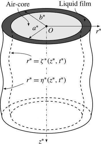
, respectively. It is convenient to describe the geometry and dynamics of the system in cylindrical polar coordinates, as illustrated in figure 1. The instantaneous locations of the free surface and liquid–wall interface are denoted by
 $r^{\ast }=\unicode[STIX]{x1D701}^{\ast }(z^{\ast },t^{\ast })$
and
 $r^{\ast }=\unicode[STIX]{x1D702}^{\ast }(z^{\ast },t^{\ast })$
.
Geometry of an annular liquid film flowing down the inner surface of a flexible tube.

The governing equations are the continuity equation and Navier–Stokes equations:
 $$\begin{eqnarray}\displaystyle & \displaystyle \unicode[STIX]{x1D735}^{\ast }\boldsymbol{\cdot }\boldsymbol{V}^{\ast }=0, & \displaystyle\end{eqnarray}$$
 $$\begin{eqnarray}\displaystyle & \displaystyle \unicode[STIX]{x1D70C}^{\ast }\left(\frac{\unicode[STIX]{x2202}\boldsymbol{V}^{\ast }}{\unicode[STIX]{x2202}t^{\ast }}+\boldsymbol{V}^{\ast }\boldsymbol{\cdot }\unicode[STIX]{x1D735}^{\ast }\boldsymbol{V}^{\ast }\right)=-\unicode[STIX]{x1D735}^{\ast }p^{\ast }+\unicode[STIX]{x1D735}^{\ast }\boldsymbol{\cdot }\unicode[STIX]{x1D749}^{\ast }+\unicode[STIX]{x1D70C}^{\ast }g^{\ast }\boldsymbol{e}_{z}, & \displaystyle\end{eqnarray}$$
 $\unicode[STIX]{x1D70C}^{\ast }$
,
 $\boldsymbol{V}^{\ast }$
,
 $p^{\ast }$
and
 $\unicode[STIX]{x1D749}^{\ast }$
are the density, velocity vector, pressure and stress tensor of the annular film flow, and
 $\boldsymbol{e}_{z}$
is the unit vector along the
 $z^{\ast }$
-axis. The upper-convected Maxwell (UCM) constitutive equation is adopted to model the viscoelastic behaviour of the liquid, which has been widely used for various flows:
 $$\begin{eqnarray}\unicode[STIX]{x1D749}^{\ast }+\unicode[STIX]{x1D706}^{\ast }\frac{\unicode[STIX]{x1D6FF}\unicode[STIX]{x1D749}^{\ast }}{\unicode[STIX]{x1D6FF}t^{\ast }}=\unicode[STIX]{x1D707}^{\ast }(\unicode[STIX]{x1D735}^{\ast }\boldsymbol{V}+(\unicode[STIX]{x1D735}^{\ast }\boldsymbol{V})^{\top }).\end{eqnarray}$$
Here,
 $\unicode[STIX]{x1D706}^{\ast }$
is the relaxation time, and
 $\unicode[STIX]{x1D707}^{\ast }$
is the polymer-contributed viscosity of the UCM fluid. Obviously, the UCM model can be reduced to the Newtonian fluid model by letting
 $\unicode[STIX]{x1D706}^{\ast }=0$
. The upper-convected derivative in equation (2.2) is given by
 $$\begin{eqnarray}\frac{\unicode[STIX]{x1D6FF}\unicode[STIX]{x1D749}^{\ast }}{\unicode[STIX]{x1D6FF}t^{\ast }}=\frac{\unicode[STIX]{x2202}\unicode[STIX]{x1D749}^{\ast }}{\unicode[STIX]{x2202}t^{\ast }}+\boldsymbol{V}^{\ast }\boldsymbol{\cdot }\unicode[STIX]{x1D735}^{\ast }\unicode[STIX]{x1D749}^{\ast }-(\unicode[STIX]{x1D735}^{\ast }\boldsymbol{V}^{\ast })^{\top }\boldsymbol{\cdot }\unicode[STIX]{x1D749}^{\ast }-\unicode[STIX]{x1D749}^{\ast }\boldsymbol{\cdot }\unicode[STIX]{x1D735}^{\ast }\boldsymbol{V}^{\ast }.\end{eqnarray}$$
At the free surface,
 $r^{\ast }=\unicode[STIX]{x1D701}^{\ast }(z^{\ast },t^{\ast })$
, the kinematic boundary condition is
 $$\begin{eqnarray}\unicode[STIX]{x1D701}_{t}^{\ast }-V_{r}^{\ast }+V_{z}^{\ast }\unicode[STIX]{x1D701}_{z}^{\ast }=0,\end{eqnarray}$$
where
 $\unicode[STIX]{x1D701}_{t}^{\ast }=\unicode[STIX]{x2202}\unicode[STIX]{x1D701}^{\ast }/\unicode[STIX]{x2202}t^{\ast }$
,
 $\unicode[STIX]{x1D701}_{z}^{\ast }=\unicode[STIX]{x2202}\unicode[STIX]{x1D701}^{\ast }/\unicode[STIX]{x2202}z^{\ast }$
, and
 $V_{r}^{\ast }$
and
 $V_{z}^{\ast }$
are the radial and axial flow velocity components, respectively. Moreover, we have the balances of tangential and normal stresses:
 $$\begin{eqnarray}\displaystyle & \displaystyle \unicode[STIX]{x1D701}_{z}^{\ast }(\unicode[STIX]{x1D70F}_{rr}^{\ast }-\unicode[STIX]{x1D70F}_{zz}^{\ast })+[1-(\unicode[STIX]{x1D701}_{z}^{\ast })^{2}]\unicode[STIX]{x1D70F}_{rz}^{\ast }=0, & \displaystyle\end{eqnarray}$$
 $$\begin{eqnarray}\displaystyle & \displaystyle \unicode[STIX]{x1D70F}_{rr}^{\ast }-2\unicode[STIX]{x1D701}_{z}^{\ast }\unicode[STIX]{x1D70F}_{rz}^{\ast }+(\unicode[STIX]{x1D701}_{z}^{\ast })^{2}\unicode[STIX]{x1D70F}_{zz}^{\ast }=[1+(\unicode[STIX]{x1D701}_{z}^{\ast })^{2}](p^{\ast }-p_{in}^{\ast })-\unicode[STIX]{x1D6FE}^{\ast }\left(\frac{\unicode[STIX]{x1D701}_{z,z}^{\ast }}{\unicode[STIX]{x1D6E5}_{\unicode[STIX]{x1D701}}^{\ast }}-\frac{\unicode[STIX]{x1D6E5}_{\unicode[STIX]{x1D701}}^{\ast }}{\unicode[STIX]{x1D701}^{\ast }}\right). & \displaystyle\end{eqnarray}$$
 $\unicode[STIX]{x1D6E5}_{\unicode[STIX]{x1D701}}^{\ast }=\sqrt{1+(\unicode[STIX]{x1D701}_{z}^{\ast })^{2}}$
,
 $\unicode[STIX]{x1D701}_{z,z}^{\ast }=\unicode[STIX]{x2202}^{2}\unicode[STIX]{x1D701}^{\ast }/\unicode[STIX]{x2202}{z^{\ast }}^{2}$
,
 $\unicode[STIX]{x1D6FE}^{\ast }$
is the surface tension, and
 $\unicode[STIX]{x1D70F}_{rr}^{\ast }$
,
 $\unicode[STIX]{x1D70F}_{rz}^{\ast }$
and
 $\unicode[STIX]{x1D70F}_{zz}^{\ast }$
are the components of the stress tensor
 $\unicode[STIX]{x1D749}^{\ast }$
.
At the wall of the flexible tube,
 $r^{\ast }=\unicode[STIX]{x1D702}^{\ast }(z^{\ast },t^{\ast })$
, the kinematic boundary condition is
 $$\begin{eqnarray}\unicode[STIX]{x1D702}_{t}^{\ast }-V_{r}^{\ast }+V_{z}^{\ast }\unicode[STIX]{x1D702}_{z}^{\ast }=0.\end{eqnarray}$$
In this study, the flexible tube is assumed to be tethered, and the deflection of the tube along the axial direction is ignored. Thus, we have the no-slip condition
 $V_{z}^{\ast }(\unicode[STIX]{x1D702}^{\ast },t^{\ast })=0$
. The kinematic boundary condition can be simplified as
 $\unicode[STIX]{x1D702}_{t}^{\ast }=V_{r}^{\ast }$
. Following Halpern & Grotberg (Reference Halpern and Grotberg1992), the equation of equilibrium of normal stress is given by
 $$\begin{eqnarray}\frac{\unicode[STIX]{x1D6FC}^{\ast }\unicode[STIX]{x1D70C}_{w}^{\ast }H_{w}^{\ast }\unicode[STIX]{x1D702}_{t}^{\ast }}{\unicode[STIX]{x1D6E5}_{\unicode[STIX]{x1D702}}^{\ast }}+\frac{T_{\unicode[STIX]{x1D703}}^{\ast }}{\unicode[STIX]{x1D702}^{\ast }\unicode[STIX]{x1D6E5}_{\unicode[STIX]{x1D702}}^{\ast }}-\frac{T_{z}^{\ast }\unicode[STIX]{x1D702}_{z,z}^{\ast }}{(\unicode[STIX]{x1D6E5}_{\unicode[STIX]{x1D702}}^{\ast })^{3}}=p^{\ast }-p_{out}^{\ast }-\frac{1}{1+(\unicode[STIX]{x1D702}_{z}^{\ast })^{2}}[\unicode[STIX]{x1D70F}_{rr}^{\ast }-2\unicode[STIX]{x1D702}_{z}^{\ast }\unicode[STIX]{x1D70F}_{rz}^{\ast }+(\unicode[STIX]{x1D702}_{z}^{\ast })^{2}\unicode[STIX]{x1D70F}_{zz}^{\ast }],\end{eqnarray}$$
where
 $\unicode[STIX]{x1D6E5}_{\unicode[STIX]{x1D702}}^{\ast }=\sqrt{1+(\unicode[STIX]{x1D702}_{z}^{\ast })^{2}}$
. The relevant characteristics of the tube wall are its damping coefficient
 $\unicode[STIX]{x1D6FC}^{\ast }$
, density
 $\unicode[STIX]{x1D70C}_{w}^{\ast }$
, thickness
 $H_{w}^{\ast }$
, longitudinal tension
 $T_{z}^{\ast }$
and circumferential tension
 $T_{\unicode[STIX]{x1D703}}^{\ast }$
. In this study,
 $T_{\unicode[STIX]{x1D703}}^{\ast }$
is given as follows (Gol’Denveizer Reference Gol’Denveizer2014):
 $$\begin{eqnarray}T_{\unicode[STIX]{x1D703}}^{\ast }=T_{0}^{\ast }+\frac{E^{\ast }H_{w}^{\ast }}{1-\unicode[STIX]{x1D708}^{2}}\frac{\unicode[STIX]{x1D702}^{\ast }-b^{\ast }}{\unicode[STIX]{x1D702}^{\ast }},\end{eqnarray}$$
where
 $E^{\ast }$
is the modulus of elasticity,
 $\unicode[STIX]{x1D708}$
is the Poisson’s ratio and
 $T_{0}^{\ast }$
indicates the initial tension.
According to equations (2.1)–(2.8), the base flow of the viscoelastic fluid film can be easily derived as follows:
 $$\begin{eqnarray}\overline{V}_{z}^{\ast }(r^{\ast })=\frac{\unicode[STIX]{x1D70C}^{\ast }g^{\ast }{b^{\ast }}^{2}}{4\unicode[STIX]{x1D707}^{\ast }}\left[1-\left(\frac{r^{\ast }}{b^{\ast }}\right)^{2}+2\left(\frac{a^{\ast }}{b^{\ast }}\right)^{2}\log \frac{r^{\ast }}{b^{\ast }}\right],\end{eqnarray}$$
 $$\begin{eqnarray}\overline{\unicode[STIX]{x1D70F}}_{rz}^{\ast }(r^{\ast })=\frac{\unicode[STIX]{x1D70C}g^{\ast }}{2r^{\ast }}({a^{\ast }}^{2}-{r^{\ast }}^{2}),\quad \overline{\unicode[STIX]{x1D70F}}_{zz}^{\ast }(r^{\ast })=2\unicode[STIX]{x1D706}^{\ast }[\overline{\unicode[STIX]{x1D70F}}_{rz}^{\ast }(r^{\ast })]^{2},\end{eqnarray}$$
 $$\begin{eqnarray}\overline{p}^{\ast }(r^{\ast })=p_{in}^{\ast }-\frac{\unicode[STIX]{x1D6FE}^{\ast }}{a^{\ast }}=p_{out}^{\ast }+\frac{1}{b^{\ast }}T_{0}^{\ast },\end{eqnarray}$$
and
 $\overline{\unicode[STIX]{x1D70F}}_{rr}^{\ast }(r^{\ast })=\overline{\unicode[STIX]{x1D70F}}_{\unicode[STIX]{x1D703}\unicode[STIX]{x1D703}}^{\ast }(r^{\ast })\equiv 0$
. The volume flow rate can be written as
 $$\begin{eqnarray}\overline{Q}^{\ast }=2\unicode[STIX]{x03C0}\int _{a^{\ast }}^{b^{\ast }}r^{\ast }\overline{V}_{z}^{\ast }(r^{\ast })\,\text{d}r^{\ast }=2\unicode[STIX]{x03C0}\frac{\unicode[STIX]{x1D70C}^{\ast }g^{\ast }b^{\ast }{h^{\ast }}^{3}}{\unicode[STIX]{x1D707}^{\ast }}\unicode[STIX]{x1D711}(\unicode[STIX]{x1D700}_{0}),\end{eqnarray}$$
where
 $\unicode[STIX]{x1D700}_{0}=h^{\ast }/b^{\ast }$
is the initial undisturbed film relative thickness and
 $\unicode[STIX]{x1D711}$
is a function with the following definition:
 $$\begin{eqnarray}\unicode[STIX]{x1D711}(x)=\frac{1}{16x^{3}}[(1-(1-x)^{2})(1-3(1-x)^{2})-4(1-x)^{4}\log (1-x)].\end{eqnarray}$$
2.2 Non-dimensionalization
Hereinafter, the governing equations and boundary conditions are rendered dimensionless by letting
 $$\begin{eqnarray}\displaystyle \left.\begin{array}{@{}c@{}}\displaystyle t=\unicode[STIX]{x1D705}\frac{t^{\ast }}{h^{\ast }/U_{0}^{\ast }},\quad \{z,r\}=\frac{1}{h^{\ast }}\{\unicode[STIX]{x1D705}z^{\ast },r^{\ast }\},\quad \{V_{z},V_{r}\}=\frac{1}{U_{0}^{\ast }}\left\{V_{z}^{\ast },\frac{1}{\unicode[STIX]{x1D705}}V_{r}^{\ast }\right\},\\ \displaystyle p=\frac{p^{\ast }}{\unicode[STIX]{x1D70C}^{\ast }{U_{0}^{\ast }}^{2}},\quad \{\unicode[STIX]{x1D70F}_{rr},\unicode[STIX]{x1D70F}_{\unicode[STIX]{x1D703}\unicode[STIX]{x1D703}},\unicode[STIX]{x1D70F}_{zz},\unicode[STIX]{x1D70F}_{rz}\}=\frac{h^{\ast }}{\unicode[STIX]{x1D707}^{\ast }U_{0}^{\ast }}\left\{\frac{1}{\unicode[STIX]{x1D705}}\unicode[STIX]{x1D70F}_{rr}^{\ast },\frac{1}{\unicode[STIX]{x1D705}}\unicode[STIX]{x1D70F}_{\unicode[STIX]{x1D703}\unicode[STIX]{x1D703}}^{\ast },\unicode[STIX]{x1D705}\unicode[STIX]{x1D70F}_{rz}^{\ast },\unicode[STIX]{x1D70F}_{rz}^{\ast }\right\}.\end{array}\right\} & & \displaystyle\end{eqnarray}$$
Here,
 $\unicode[STIX]{x1D705}$
is a stretching parameter,
 $h^{\ast }$
is the equilibrium film thickness and
 $U_{0}^{\ast }$
is the reference velocity defined as
 $$\begin{eqnarray}U_{0}^{\ast }=\frac{\overline{Q}^{\ast }}{2\unicode[STIX]{x03C0}b^{\ast }h^{\ast }}=\frac{\unicode[STIX]{x1D70C}^{\ast }g^{\ast }{h^{\ast }}^{2}}{\unicode[STIX]{x1D707}^{\ast }}\unicode[STIX]{x1D711}(\unicode[STIX]{x1D700}_{0}).\end{eqnarray}$$
When
 $\unicode[STIX]{x1D700}_{0}\rightarrow 0$
, it equals the average velocity of the cross-section, since the cross-sectional area tends to
 $2\unicode[STIX]{x03C0}b^{\ast }h^{\ast }$
. In this study, we aim to model the dynamics of interfacial long waves. Thus, the definition of the stretching parameter
 $\unicode[STIX]{x1D705}$
is
 $\unicode[STIX]{x1D705}=h^{\ast }/\unicode[STIX]{x1D6EC}^{\ast }\ll 1$
, where
 $\unicode[STIX]{x1D6EC}^{\ast }$
represents the wavelength of a typical coherent wave structure (Matar et al.
Reference Matar, Craster and Kumar2007). A group of dimensionless parameters can be introduced as follows:
 $$\begin{eqnarray}\displaystyle \left.\begin{array}{@{}c@{}}\displaystyle Re=\frac{\unicode[STIX]{x1D70C}^{\ast }U_{0}^{\ast }h^{\ast }}{\unicode[STIX]{x1D707}^{\ast }},\quad We=\frac{\unicode[STIX]{x1D70C}^{\ast }{U_{0}^{\ast }}^{2}h^{\ast }}{\unicode[STIX]{x1D6FE}^{\ast }},\quad De=\frac{\unicode[STIX]{x1D706}^{\ast }U_{0}^{\ast }}{h^{\ast }},\\ \displaystyle \unicode[STIX]{x1D6FC}=\frac{\unicode[STIX]{x1D6FC}^{\ast }\unicode[STIX]{x1D70C}_{w}^{\ast }H_{w}^{\ast }}{\unicode[STIX]{x1D6FE}^{\ast }/(U_{0}^{\ast }h^{\ast })},\quad \unicode[STIX]{x1D6FD}=\frac{E^{\ast }H_{w}^{\ast }}{(1-\unicode[STIX]{x1D708}^{2})\unicode[STIX]{x1D6FE}^{\ast }},\quad \{T_{0},T_{z}\}=\frac{1}{\unicode[STIX]{x1D6FE}^{\ast }}\{T_{0}^{\ast },T_{z}^{\ast }\}.\end{array}\right\} & & \displaystyle\end{eqnarray}$$
Here,
 $Re$
is the Reynolds number and
 $We$
denotes the Weber number;
 $De$
is the Deborah number, which indicates the ratio of the time scales corresponding to the viscoelastic effects and hydrodynamic flow;
 $\unicode[STIX]{x1D6FC}$
represents the ratio between the damping effect of the flexible tube and the effect of the surface tension; and
 $\unicode[STIX]{x1D6FD}$
represents the ratio of the hoop elastic forces to the surface tension.
In order to retain the effects of surface tension, gravity, viscoelasticity and flexible tube at the leading order (Matar et al. Reference Matar, Craster and Kumar2007), the above parameters are rescaled as follows:
 $$\begin{eqnarray}\{\widehat{Re},\widehat{De}\}=\unicode[STIX]{x1D705}\{Re,De\},\quad \widehat{We}=We/\unicode[STIX]{x1D705}^{2},\quad \widehat{\unicode[STIX]{x1D6FC}}=\unicode[STIX]{x1D6FC}/\unicode[STIX]{x1D705}.\end{eqnarray}$$
By substituting equations (2.12)–(2.15) into (2.1) with leading order
 $O(\unicode[STIX]{x1D705})$
, we have
 $$\begin{eqnarray}\displaystyle & \displaystyle \frac{\unicode[STIX]{x2202}V_{r}}{\unicode[STIX]{x2202}r}+\frac{\unicode[STIX]{x2202}V_{z}}{\unicode[STIX]{x2202}z}+\frac{V_{r}}{r}=0, & \displaystyle\end{eqnarray}$$
 $$\begin{eqnarray}\displaystyle & \displaystyle 0=-\frac{\unicode[STIX]{x2202}p}{\unicode[STIX]{x2202}r}, & \displaystyle\end{eqnarray}$$
 $$\begin{eqnarray}\displaystyle & \displaystyle \frac{\unicode[STIX]{x2202}V_{z}}{\unicode[STIX]{x2202}t}+V_{r}\frac{\unicode[STIX]{x2202}V_{z}}{\unicode[STIX]{x2202}r}+V_{z}\frac{\unicode[STIX]{x2202}V_{z}}{\unicode[STIX]{x2202}z}=-\frac{\unicode[STIX]{x2202}p}{\unicode[STIX]{x2202}z}+\frac{1}{\widehat{Re}}\left(\frac{\unicode[STIX]{x2202}\unicode[STIX]{x1D70F}_{rz}}{\unicode[STIX]{x2202}r}+\frac{\unicode[STIX]{x2202}\unicode[STIX]{x1D70F}_{zz}}{\unicode[STIX]{x2202}z}+\frac{\unicode[STIX]{x1D70F}_{rz}}{r}\right)+\frac{1}{\widehat{Re}\unicode[STIX]{x1D711}(\unicode[STIX]{x1D700}_{0})}. & \displaystyle\end{eqnarray}$$
 $\unicode[STIX]{x1D705}\ll 1$
. The boundary conditions at the free surface yield
 $$\begin{eqnarray}\displaystyle & \displaystyle \unicode[STIX]{x1D701}_{t}-V_{r}+V_{z}\unicode[STIX]{x1D701}_{z}=0, & \displaystyle\end{eqnarray}$$
 $$\begin{eqnarray}\displaystyle & \displaystyle \unicode[STIX]{x1D70F}_{rz}-\unicode[STIX]{x1D701}_{z}\unicode[STIX]{x1D70F}_{zz}=0, & \displaystyle\end{eqnarray}$$
 $$\begin{eqnarray}\displaystyle & \displaystyle p-p_{in}=\frac{1}{\widehat{We}}\left(\unicode[STIX]{x1D701}_{z,z}-\frac{1}{\unicode[STIX]{x1D705}^{2}\unicode[STIX]{x1D701}}\right). & \displaystyle\end{eqnarray}$$
 $$\begin{eqnarray}\displaystyle & \displaystyle V_{r}=\unicode[STIX]{x1D702}_{t},\quad V_{z}=0, & \displaystyle\end{eqnarray}$$
 $$\begin{eqnarray}\displaystyle & \displaystyle \widehat{\unicode[STIX]{x1D6FC}}\unicode[STIX]{x1D702}_{t}+\frac{1}{\unicode[STIX]{x1D705}^{2}}\frac{1}{\unicode[STIX]{x1D702}}\left(T_{0}+\unicode[STIX]{x1D6FD}\frac{\unicode[STIX]{x1D702}-b}{\unicode[STIX]{x1D702}}\right)-T_{z}\unicode[STIX]{x1D702}_{z,z}=\widehat{We}(p-p_{out}). & \displaystyle\end{eqnarray}$$
 $$\begin{eqnarray}p-p_{out}=(p-p_{in})+(p_{in}-p_{out})=\frac{1}{\widehat{We}}\left[\unicode[STIX]{x1D701}_{z,z}+\frac{1}{\unicode[STIX]{x1D705}^{2}}\left(\frac{1}{a}-\frac{1}{\unicode[STIX]{x1D701}}\right)+\frac{T_{0}}{b}\right].\end{eqnarray}$$
By substituting equation (2.12) into (2.2)–(2.3), we have the dimensionless constitutive equations as follows:
 $$\begin{eqnarray}\displaystyle & \displaystyle \unicode[STIX]{x1D70F}_{rr}+\widehat{De}\mathscr{L}(\unicode[STIX]{x1D70F}_{rr})-2\widehat{De}\left(\unicode[STIX]{x1D70F}_{rr}\frac{\unicode[STIX]{x2202}V_{r}}{\unicode[STIX]{x2202}r}+\unicode[STIX]{x1D70F}_{rz}\frac{\unicode[STIX]{x2202}V_{r}}{\unicode[STIX]{x2202}z}\right)=2\frac{\unicode[STIX]{x2202}V_{r}}{\unicode[STIX]{x2202}r}, & \displaystyle\end{eqnarray}$$
 $$\begin{eqnarray}\displaystyle & \displaystyle \unicode[STIX]{x1D70F}_{\unicode[STIX]{x1D703}\unicode[STIX]{x1D703}}+\widehat{De}\mathscr{L}(\unicode[STIX]{x1D70F}_{\unicode[STIX]{x1D703}\unicode[STIX]{x1D703}})-2\widehat{De}\frac{V_{r}}{r}\unicode[STIX]{x1D70F}_{\unicode[STIX]{x1D703}\unicode[STIX]{x1D703}}=2\frac{V_{r}}{r}, & \displaystyle\end{eqnarray}$$
 $$\begin{eqnarray}\displaystyle & \displaystyle \unicode[STIX]{x1D70F}_{zz}+\widehat{De}\mathscr{L}(\unicode[STIX]{x1D70F}_{zz})-2\widehat{De}\left(\unicode[STIX]{x1D70F}_{rz}\frac{\unicode[STIX]{x2202}V_{z}}{\unicode[STIX]{x2202}r}+\unicode[STIX]{x1D70F}_{zz}\frac{\unicode[STIX]{x2202}V_{z}}{\unicode[STIX]{x2202}z}\right)=2\unicode[STIX]{x1D705}^{2}\frac{\unicode[STIX]{x2202}V_{z}}{\unicode[STIX]{x2202}z}, & \displaystyle\end{eqnarray}$$
 $$\begin{eqnarray}\displaystyle & & \displaystyle \unicode[STIX]{x1D70F}_{rz}+\widehat{De}\mathscr{L}(\unicode[STIX]{x1D70F}_{rz})-\widehat{De}\left(\unicode[STIX]{x1D70F}_{rr}\frac{\unicode[STIX]{x2202}V_{z}}{\unicode[STIX]{x2202}r}+\unicode[STIX]{x1D70F}_{rz}\frac{\unicode[STIX]{x2202}V_{z}}{\unicode[STIX]{x2202}z}\right)\nonumber\\ \displaystyle & & \displaystyle \quad -\,\widehat{De}\left(\unicode[STIX]{x1D70F}_{rz}\frac{\unicode[STIX]{x2202}V_{r}}{\unicode[STIX]{x2202}r}+\unicode[STIX]{x1D70F}_{zz}\frac{\unicode[STIX]{x2202}V_{r}}{\unicode[STIX]{x2202}z}\right)=\unicode[STIX]{x1D705}^{2}\frac{\unicode[STIX]{x2202}V_{r}}{\unicode[STIX]{x2202}z}+\frac{\unicode[STIX]{x2202}V_{z}}{\unicode[STIX]{x2202}r},\end{eqnarray}$$
where the differential operator
 $\mathscr{L}$
is defined as
 $\mathscr{L}=\unicode[STIX]{x2202}_{t}+V_{r}\unicode[STIX]{x2202}_{r}+V_{z}\unicode[STIX]{x2202}_{z}$
. In this study, we consider the liquid with weak viscoelasticity (i.e.
 $\widehat{De}=\unicode[STIX]{x1D705}De\ll 1$
). Then, we can expand the stresses in terms of
 $\widehat{De}$
:
 $$\begin{eqnarray}\unicode[STIX]{x1D749}=\unicode[STIX]{x1D749}^{(0)}+\widehat{De}\unicode[STIX]{x1D749}^{(1)}+O(\widehat{De})^{2}.\end{eqnarray}$$
Similar to Saprykin et al. (Reference Saprykin, Koopmans and Kalliadasis2007), by substituting (2.21) into (2.20d
) with leading order
 $O(\unicode[STIX]{x1D705},\widehat{De})$
, the explicit approximation expressions for the stresses can be written as follows:
 $$\begin{eqnarray}\displaystyle & \displaystyle \unicode[STIX]{x1D70F}_{rr}=2\frac{\unicode[STIX]{x2202}V_{r}}{\unicode[STIX]{x2202}r}+\widehat{De}\left[4\left(\frac{\unicode[STIX]{x2202}V_{r}}{\unicode[STIX]{x2202}r}\right)^{2}+2\frac{\unicode[STIX]{x2202}V_{z}}{\unicode[STIX]{x2202}r}\frac{\unicode[STIX]{x2202}V_{r}}{\unicode[STIX]{x2202}z}-2\mathscr{L}\left(\frac{\unicode[STIX]{x2202}V_{r}}{\unicode[STIX]{x2202}r}\right)\right], & \displaystyle\end{eqnarray}$$
 $$\begin{eqnarray}\displaystyle & \displaystyle \unicode[STIX]{x1D70F}_{\unicode[STIX]{x1D703}\unicode[STIX]{x1D703}}=2\frac{V_{r}}{r}+\widehat{De}\left[4\left(\frac{V_{r}}{r}\right)^{2}-2\mathscr{L}\left(\frac{V_{r}}{r}\right)\right], & \displaystyle\end{eqnarray}$$
 $$\begin{eqnarray}\displaystyle & \displaystyle \unicode[STIX]{x1D70F}_{zz}=2\widehat{De}\left(\frac{\unicode[STIX]{x2202}V_{z}}{\unicode[STIX]{x2202}r}\right)^{2}, & \displaystyle\end{eqnarray}$$
 $$\begin{eqnarray}\displaystyle & \displaystyle \unicode[STIX]{x1D70F}_{rz}=\frac{\unicode[STIX]{x2202}V_{z}}{\unicode[STIX]{x2202}r}+\widehat{De}\left[3\frac{\unicode[STIX]{x2202}V_{r}}{\unicode[STIX]{x2202}r}\frac{\unicode[STIX]{x2202}V_{z}}{\unicode[STIX]{x2202}z}+\frac{\unicode[STIX]{x2202}V_{z}}{\unicode[STIX]{x2202}r}\frac{\unicode[STIX]{x2202}V_{z}}{\unicode[STIX]{x2202}z}-\mathscr{L}\left(\frac{\unicode[STIX]{x2202}V_{z}}{\unicode[STIX]{x2202}r}\right)\right]. & \displaystyle\end{eqnarray}$$
2.3 Evolution equations
In this section, the integral theory is adopted to derive the evolution equations of the liquid film and the flexible tube. The system equations presented in the previous section are required to be fulfilled on average (Ruyer-Quil & Manneville Reference Ruyer-Quil and Manneville2000). Integration of the continuity equation (2.16a
) from
 $r=\unicode[STIX]{x1D701}(z,t)$
to
 $r=\unicode[STIX]{x1D702}(z,t)$
, evaluating by applying the kinematic condition at the free surface (2.17a
) and the no-slip condition at the liquid–wall interface (2.18a
), yields
 $$\begin{eqnarray}\frac{1}{2}\frac{\unicode[STIX]{x2202}}{\unicode[STIX]{x2202}t}(\unicode[STIX]{x1D701}^{2}-\unicode[STIX]{x1D702}^{2})=\frac{\unicode[STIX]{x2202}q}{\unicode[STIX]{x2202}z},\end{eqnarray}$$
where
 $$\begin{eqnarray}q(z,t)=\int _{\unicode[STIX]{x1D701}(z,t)}^{\unicode[STIX]{x1D702}(z,t)}rV_{z}(r,z,t)\,\text{d}r\end{eqnarray}$$
denotes the volume flow rate divided by
 $2\unicode[STIX]{x03C0}$
. In order to integrate the axial momentum equation (2.16c
), the axial velocity profile, which satisfies the boundary condition (2.17b
) at the free surface and the no-slip condition (2.18a
) at the liquid–wall interface, is assumed to be of the form
 $$\begin{eqnarray}V_{z}(r)=\frac{q(z,t)}{4\unicode[STIX]{x1D711}(\unicode[STIX]{x1D700})h^{3}\unicode[STIX]{x1D702}}\left(\unicode[STIX]{x1D702}^{2}-r^{2}+2\unicode[STIX]{x1D701}^{2}\log \frac{r}{\unicode[STIX]{x1D702}}\right).\end{eqnarray}$$
Here,
 $h(z,t)=\unicode[STIX]{x1D702}(z,t)-\unicode[STIX]{x1D701}(z,t)$
is the instantaneous dimensionless thickness,
 $\unicode[STIX]{x1D700}(z,t)=h(z,t)/\unicode[STIX]{x1D702}(z,t)$
is the instantaneous relative thickness and the function
 $\unicode[STIX]{x1D711}$
is defined in equation (2.11). Integration of the axial momentum equation (2.16c
) from
 $r=\unicode[STIX]{x1D701}(z,t)$
to
 $r=\unicode[STIX]{x1D702}(z,t)$
, evaluating by applying the boundary conditions in (2.17) and (2.18), yields
 $$\begin{eqnarray}\frac{\unicode[STIX]{x2202}q}{\unicode[STIX]{x2202}t}+\frac{\unicode[STIX]{x2202}M}{\unicode[STIX]{x2202}z}=\unicode[STIX]{x1D6F7}+\unicode[STIX]{x1D6F9}+\unicode[STIX]{x1D6F1}_{1}+\unicode[STIX]{x1D6F1}_{2},\end{eqnarray}$$
where
 $$\begin{eqnarray}\displaystyle & \displaystyle M=\int _{\unicode[STIX]{x1D701}(z,t)}^{\unicode[STIX]{x1D702}(z,t)}rV_{z}^{2}(r)\,\text{d}r=\frac{\unicode[STIX]{x1D719}(1-\unicode[STIX]{x1D700})}{16\unicode[STIX]{x1D700}^{5}\unicode[STIX]{x1D711}^{2}(\unicode[STIX]{x1D700})}\frac{q^{2}}{h\unicode[STIX]{x1D702}}, & \displaystyle\end{eqnarray}$$
 $$\begin{eqnarray}\displaystyle & \displaystyle \unicode[STIX]{x1D6F7}=\int _{\unicode[STIX]{x1D701}(z,t)}^{\unicode[STIX]{x1D702}(z,t)}\frac{1}{\unicode[STIX]{x1D711}(\unicode[STIX]{x1D700}_{0})\widehat{Re}}r\,\text{d}r=h\unicode[STIX]{x1D702}\left(1-\frac{\unicode[STIX]{x1D700}}{2}\right)\frac{1}{\unicode[STIX]{x1D711}(\unicode[STIX]{x1D700}_{0})\widehat{Re}}, & \displaystyle\end{eqnarray}$$
 $$\begin{eqnarray}\displaystyle & \displaystyle \unicode[STIX]{x1D6F9}=\int _{\unicode[STIX]{x1D701}(z,t)}^{\unicode[STIX]{x1D702}(z,t)}-\frac{\unicode[STIX]{x2202}p}{\unicode[STIX]{x2202}z}r\,\text{d}r=-h\unicode[STIX]{x1D702}\left(1-\frac{\unicode[STIX]{x1D700}}{2}\right)\frac{1}{\widehat{We}}\left(\frac{\unicode[STIX]{x2202}^{3}\unicode[STIX]{x1D701}}{\unicode[STIX]{x2202}z^{3}}+\frac{1}{\unicode[STIX]{x1D705}^{2}\unicode[STIX]{x1D701}^{2}}\frac{\unicode[STIX]{x2202}\unicode[STIX]{x1D701}}{\unicode[STIX]{x2202}z}\right), & \displaystyle\end{eqnarray}$$
 $$\begin{eqnarray}\displaystyle & \displaystyle \unicode[STIX]{x1D6F1}_{1}=\int _{\unicode[STIX]{x1D701}(z,t)}^{\unicode[STIX]{x1D702}(z,t)}\frac{1}{r}\frac{\unicode[STIX]{x2202}(r\unicode[STIX]{x1D70F}_{rz})}{\unicode[STIX]{x2202}r}r\,\text{d}r=\frac{1}{\unicode[STIX]{x1D711}(\unicode[STIX]{x1D700}_{0})\widehat{Re}}\left[\widehat{De}\left(\frac{\unicode[STIX]{x2202}L}{\unicode[STIX]{x2202}t}+J\frac{\unicode[STIX]{x2202}\unicode[STIX]{x1D702}}{\unicode[STIX]{x2202}t}+K\frac{\unicode[STIX]{x2202}\unicode[STIX]{x1D702}}{\unicode[STIX]{x2202}z}\right)-L\right], & \displaystyle\end{eqnarray}$$
 $$\begin{eqnarray}\displaystyle & \displaystyle \unicode[STIX]{x1D6F1}_{2}=\int _{\unicode[STIX]{x1D701}(z,t)}^{\unicode[STIX]{x1D702}(z,t)}\frac{\unicode[STIX]{x2202}\unicode[STIX]{x1D70F}_{zz}}{\unicode[STIX]{x2202}r}r\,\text{d}r=\frac{\widehat{De}}{\unicode[STIX]{x1D711}(\unicode[STIX]{x1D700}_{0})\widehat{Re}}\left(\frac{\unicode[STIX]{x2202}N}{\unicode[STIX]{x2202}z}-K\frac{\unicode[STIX]{x2202}\unicode[STIX]{x1D702}}{\unicode[STIX]{x2202}z}\right). & \displaystyle\end{eqnarray}$$
 $L$
,
 $N$
,
 $J$
and
 $K$
are listed in appendix A, and
 $\unicode[STIX]{x1D719}$
is a function defined as
 $$\begin{eqnarray}\unicode[STIX]{x1D719}(x)=-{\textstyle \frac{17}{12}}x^{6}+{\textstyle \frac{5}{2}}x^{4}-{\textstyle \frac{5}{4}}x^{2}+{\textstyle \frac{1}{6}}-x^{4}\log x\cdot (2-3x^{2}+2x^{2}\log x).\end{eqnarray}$$
According to (2.27), clearly,
 $M$
represents the contribution of the fluid inertial;
 $\unicode[STIX]{x1D6F7}$
indicates the contribution of gravity;
 $\unicode[STIX]{x1D6F9}$
represents the contribution of surface tension;
 $\unicode[STIX]{x1D6F1}_{1}$
denotes the contribution of the wall shear stress caused by the fluid elasticity and viscosity; and
 $\unicode[STIX]{x1D6F1}_{2}$
denotes the contribution of the
 $z$
-directed normal stress of the viscoelastic fluid. In order to clarify the contributions of surface tensions and fluid viscoelasticity, we introduce
 $$\begin{eqnarray}\displaystyle \unicode[STIX]{x1D6F1}=\unicode[STIX]{x1D6F1}_{1}+\unicode[STIX]{x1D6F1}_{2}+\frac{L}{\unicode[STIX]{x1D711}(\unicode[STIX]{x1D700}_{0})\widehat{Re}}=\frac{\widehat{De}}{\unicode[STIX]{x1D711}(\unicode[STIX]{x1D700}_{0})\widehat{Re}}\left(\frac{\unicode[STIX]{x2202}L}{\unicode[STIX]{x2202}t}+J\frac{\unicode[STIX]{x2202}\unicode[STIX]{x1D702}}{\unicode[STIX]{x2202}t}+\frac{\unicode[STIX]{x2202}N}{\unicode[STIX]{x2202}z}\right), & & \displaystyle\end{eqnarray}$$
 $$\begin{eqnarray}\displaystyle \unicode[STIX]{x1D6F9}_{z}=-h\unicode[STIX]{x1D702}\left(1-\frac{\unicode[STIX]{x1D700}}{2}\right)\frac{1}{\widehat{We}}\frac{\unicode[STIX]{x2202}^{3}\unicode[STIX]{x1D701}}{\unicode[STIX]{x2202}z^{3}},\quad \unicode[STIX]{x1D6F9}_{r}=-h\unicode[STIX]{x1D702}\left(1-\frac{\unicode[STIX]{x1D700}}{2}\right)\frac{1}{\widehat{We}}\frac{1}{\unicode[STIX]{x1D705}^{2}\unicode[STIX]{x1D701}^{2}}\frac{\unicode[STIX]{x2202}\unicode[STIX]{x1D701}}{\unicode[STIX]{x2202}z}. & & \displaystyle\end{eqnarray}$$
 $\unicode[STIX]{x1D6F1}$
represents the contribution of fluid viscoelasticity. The contribution of the wall shear stress caused by the fluid viscosity (
 $-(\unicode[STIX]{x1D711}(\unicode[STIX]{x1D700}_{0})\widehat{Re})^{-1}L$
) is separated from
 $\unicode[STIX]{x1D6F1}_{1}$
,
 $\unicode[STIX]{x1D6F9}_{z}$
represents the contribution of longitudinal surface tension, while
 $\unicode[STIX]{x1D6F9}_{r}$
represents the contribution of circumferential surface tension. The evolution equation of the flexible tube can be reduced to
 $$\begin{eqnarray}\widehat{\unicode[STIX]{x1D6FC}}\frac{\unicode[STIX]{x2202}\unicode[STIX]{x1D702}}{\unicode[STIX]{x2202}t}=T_{z}\frac{\unicode[STIX]{x2202}^{2}\unicode[STIX]{x1D702}}{\unicode[STIX]{x2202}z^{2}}-\frac{1}{\unicode[STIX]{x1D705}^{2}}T_{0}\left(\frac{1}{\unicode[STIX]{x1D702}}-\frac{1}{b}\right)-\frac{1}{\unicode[STIX]{x1D705}^{2}}\unicode[STIX]{x1D6FD}\frac{\unicode[STIX]{x1D702}-b}{\unicode[STIX]{x1D702}^{2}}+\frac{\unicode[STIX]{x2202}^{2}\unicode[STIX]{x1D701}}{\unicode[STIX]{x2202}z^{2}}+\frac{1}{\unicode[STIX]{x1D705}^{2}}\left(\frac{1}{a}-\frac{1}{\unicode[STIX]{x1D701}}\right).\end{eqnarray}$$
So far, the system of an annular viscoelastic liquid film flowing down the inner surface of a flexible tube consists of three coupled nonlinear evolution equations: (2.23), (2.26) and (2.30), for the location of the flexible wall
 $\unicode[STIX]{x1D702}(z,t)$
, the location of the free surface
 $\unicode[STIX]{x1D701}(z,t)$
and the flow rate
 $q(z,t)$
. The corresponding trivial solution is that the film thickness
 $h(z,t)=b-a=1$
, the relative thickness
 $\unicode[STIX]{x1D700}(z,t)=\unicode[STIX]{x1D700}_{0}=1/b$
and
 $\{\unicode[STIX]{x1D701}(z,t),\unicode[STIX]{x1D702}(z,t),q(z,t)\}=\{a,b,b\}$
.
2.4 Shkadov scaling and limiting case
In order to simplify the model further, we consider the flow with typical capillary waves, in which the contributions of gravity and surface tension are of the same order (Sisoev et al.
Reference Sisoev, Craster, Matar and Gerasimov2006). In other words,
 $\unicode[STIX]{x1D6F7}$
and
 $\unicode[STIX]{x1D6F9}$
, defined in (2.27b
) and (2.27c
), are assumed to be of the same order of magnitude. In particular, by letting
 $$\begin{eqnarray}\frac{1}{\unicode[STIX]{x1D711}(\unicode[STIX]{x1D700}_{0})\widehat{Re}}=\frac{1}{\widehat{We}},\end{eqnarray}$$
we can derive
 $\unicode[STIX]{x1D705}$
for these typical capillary waves as
 $$\begin{eqnarray}\unicode[STIX]{x1D705}=\left(\frac{\unicode[STIX]{x1D70C}^{\ast }g^{\ast }(h^{\ast })^{2}}{\unicode[STIX]{x1D6FE}^{\ast }}\right)^{1/3}.\end{eqnarray}$$
Two dimensionless parameters are introduced as follows:
 $$\begin{eqnarray}Ka=\frac{\unicode[STIX]{x1D6FE}^{\ast }}{\unicode[STIX]{x1D70C}^{\ast }(\unicode[STIX]{x1D708}^{\ast })^{4/3}(g^{\ast })^{1/3}},\quad \unicode[STIX]{x1D6FF}=\frac{1}{45(\unicode[STIX]{x1D708}^{\ast })^{2}}\left(\frac{\unicode[STIX]{x1D70C}^{\ast }(g^{\ast })^{4}(h^{\ast })^{11}}{\unicode[STIX]{x1D6FE}^{\ast }}\right)^{1/3}.\end{eqnarray}$$
Here, the Kapitza number (Kapitza & Kapitza Reference Kapitza and Kapitza1949),
 $Ka$
, only depends on the fluid properties and gravity. In this study, we consider the flow of a weak viscoelastic liquid film. Therefore, we choose
 $Ka=3376$
as an approximation, which is the Kapitza number of water at 25 degrees Celsius (Ruyer-Quil & Kalliadasis Reference Ruyer-Quil and Kalliadasis2012). The parameter
 $\unicode[STIX]{x1D6FF}$
was introduced to simplify the Reynolds number (Shkadov Reference Shkadov1977). Then we can rewrite the Reynolds number, Weber number and
 $\unicode[STIX]{x1D705}$
as
 $$\begin{eqnarray}\widehat{Re}=45\unicode[STIX]{x1D6FF}\unicode[STIX]{x1D711}(\unicode[STIX]{x1D700}_{0}),\quad \widehat{We}=45\unicode[STIX]{x1D6FF}\unicode[STIX]{x1D711}^{2}(\unicode[STIX]{x1D700}_{0}),\quad \unicode[STIX]{x1D705}=\left(\frac{(45\unicode[STIX]{x1D6FF})^{2}}{Ka^{3}}\right)^{1/11}.\end{eqnarray}$$
In this study, the typical values of the various dimensional parameters are adopted according to the flow of the liquid layer in the bronchi (Weibel Reference Weibel1963; Halpern & Grotberg Reference Halpern and Grotberg1992, Reference Halpern and Grotberg1993):
 $b^{\ast }=3{-}4~\text{mm}$
,
 $h^{\ast }=b^{\ast }-a^{\ast }=0.1{-}0.2~\text{mm}$
,
 $\unicode[STIX]{x1D70C}^{\ast }=10^{3}~\text{kg}~\text{m}^{-3}$
,
 $\unicode[STIX]{x1D707}^{\ast }=0.001~\text{Pa}~\text{s}$
,
 $\unicode[STIX]{x1D6FE}^{\ast }=72.5\times 10^{-3}~\text{N}~\text{m}^{-1}$
,
 $\unicode[STIX]{x1D70C}_{w}^{\ast }=10^{3}~\text{kg}~\text{m}^{-3}$
,
 $H_{w}^{\ast }=0.025~\text{mm}$
,
 $E_{w}^{\ast }=6\times 10^{3}~\text{Pa}$
,
 $T_{0}^{\ast }\approx 0.3~\text{N}~\text{m}^{-1}$
,
 $\unicode[STIX]{x1D708}=0.5$
,
 $\unicode[STIX]{x1D6FC}^{\ast }=2\times 10^{4}~\text{s}^{-1}$
and
 $\unicode[STIX]{x1D706}^{\ast }\approx 100~\unicode[STIX]{x03BC}\text{s}$
. Therefore,
 $\unicode[STIX]{x1D6FF}\approx 0.15$
,
 $\unicode[STIX]{x1D705}\approx 0.1$
and
 $\widehat{De}\approx 0.02$
. The value of the Reynolds number is approximately 40, where the axisymmetric assumption is still valid (Padmanaban Reference Padmanaban2006). Furthermore, the orders of magnitude for the dimensionless parameters (
 $\widehat{\unicode[STIX]{x1D6FC}}$
,
 $\unicode[STIX]{x1D6FD}$
and
 $T_{z}$
) of flexible tubes are unity.
If the unperturbed radius of the flexible tube approaches infinity, i.e.
 $b\rightarrow \infty$
, the system can be reduced to that of falling films down a flexible plane. In this case,
 $\unicode[STIX]{x1D700}=h/\unicode[STIX]{x1D702}\sim \unicode[STIX]{x1D700}_{0}=1/b\rightarrow 0$
,
 $\unicode[STIX]{x1D711}(\unicode[STIX]{x1D700}_{0})\rightarrow 1/3$
and
 $\widehat{Re}\rightarrow 15\unicode[STIX]{x1D6FF}$
,
 $\widehat{We}\rightarrow 5\unicode[STIX]{x1D6FF}$
. Introduce a coordinate transformation
 $x=z,y=b-r$
, and redefine flow rate as
 $\unicode[STIX]{x1D703}=q/b$
; then the velocity profile (2.25) approaches
 $$\begin{eqnarray}V_{x}(y)=-\frac{3\unicode[STIX]{x1D703}}{2h^{3}}(y-s)(y-s-2h)+O(b^{-1}).\end{eqnarray}$$
Here,
 $s=b-\unicode[STIX]{x1D702}$
denotes the location of the liquid–wall interface. The coupled nonlinear equations (2.23), (2.26) and (2.30) can be reduced as follows:
 $$\begin{eqnarray}\displaystyle \frac{\unicode[STIX]{x2202}h}{\unicode[STIX]{x2202}t}+\frac{\unicode[STIX]{x2202}\unicode[STIX]{x1D703}}{\unicode[STIX]{x2202}x}=0, & & \displaystyle\end{eqnarray}$$
 $$\begin{eqnarray}\displaystyle \widehat{Re}\left[\frac{\unicode[STIX]{x2202}\unicode[STIX]{x1D703}}{\unicode[STIX]{x2202}t}+\frac{6}{5}\frac{\unicode[STIX]{x2202}}{\unicode[STIX]{x2202}x}\left(\frac{\unicode[STIX]{x1D703}^{2}}{h}\right)\right] & = & \displaystyle h\left(3+\frac{\widehat{Re}}{\widehat{We}}\frac{\unicode[STIX]{x2202}^{3}(s+h)}{\unicode[STIX]{x2202}x^{3}}\right)-\frac{3\unicode[STIX]{x1D703}}{h^{2}}\nonumber\\ \displaystyle & & \displaystyle +\,3\widehat{De}\left[\frac{\unicode[STIX]{x2202}}{\unicode[STIX]{x2202}t}\left(\frac{\unicode[STIX]{x1D703}}{h^{2}}\right)-\frac{\unicode[STIX]{x1D703}}{h^{3}}\frac{\unicode[STIX]{x2202}s}{\unicode[STIX]{x2202}t}+\frac{\unicode[STIX]{x2202}}{\unicode[STIX]{x2202}x}\left(\frac{2\unicode[STIX]{x1D703}^{2}}{h^{3}}\right)\right],\end{eqnarray}$$
 $$\begin{eqnarray}\displaystyle \widehat{\unicode[STIX]{x1D6FC}}\frac{\unicode[STIX]{x2202}s}{\unicode[STIX]{x2202}t}=(1+T_{z})\frac{\unicode[STIX]{x2202}^{2}s}{\unicode[STIX]{x2202}x^{2}}+\frac{\unicode[STIX]{x2202}^{2}h}{\unicode[STIX]{x2202}x^{2}}, & & \displaystyle\end{eqnarray}$$
which are the governing equations of falling films down a flexible plane (Peng, Zhang & Zhuge Reference Peng, Zhang and Zhuge2014). Comparing them with the governing equations of falling films down a flexible tube, we find that the main difference is the contribution of surface tension. As shown in equation (2.27c
), the contribution of surface tension has two parts proportional to
 $\unicode[STIX]{x2202}^{3}\unicode[STIX]{x1D701}/\unicode[STIX]{x2202}z^{3}$
and
 $\unicode[STIX]{x1D701}^{-2}\unicode[STIX]{x2202}\unicode[STIX]{x1D701}/\unicode[STIX]{x2202}z$
, respectively. The former represents the contribution of the surface tension component along the axial direction; and the latter represents the contribution of the surface tension component along the circumferential direction, which is absent in the planar case.
3 Linear stability analysis
The linear stability analysis of the system, i.e. equations (2.23), (2.26) and (2.30), is performed by using the standard normal mode composition, where an infinitesimal perturbation is applied to the initial trivial solution. Accordingly, we assume that
 $$\begin{eqnarray}\{\unicode[STIX]{x1D701}(z,t),\unicode[STIX]{x1D702}(z,t),q(z,t)\}=\{a,b,b\}+\{\tilde{\unicode[STIX]{x1D701}},\tilde{\unicode[STIX]{x1D702}},\tilde{q}\}\exp [\text{i}(kz-\unicode[STIX]{x1D714}t)],\end{eqnarray}$$
where
 $k$
is the wavenumber of a perturbation wave, and
 $\unicode[STIX]{x1D714}_{i}=\text{Im}(\unicode[STIX]{x1D714})$
denotes the growth rate. In the limit
 $\{\tilde{\unicode[STIX]{x1D701}},\tilde{\unicode[STIX]{x1D702}},\tilde{q}\}\rightarrow \{0,0,0\}$
, the corresponding linearized governing equations are
 $$\begin{eqnarray}\displaystyle & \displaystyle \text{i}k\tilde{q}=\text{i}\unicode[STIX]{x1D714}(b\tilde{\unicode[STIX]{x1D702}}-a\tilde{\unicode[STIX]{x1D701}}), & \displaystyle\end{eqnarray}$$
 $$\begin{eqnarray}\displaystyle & \displaystyle -A_{21}\tilde{\unicode[STIX]{x1D701}}+A_{22}\tilde{\unicode[STIX]{x1D702}}+A_{23}\tilde{q}=\text{i}\unicode[STIX]{x1D714}(-B_{21}\tilde{\unicode[STIX]{x1D701}}+B_{22}\tilde{\unicode[STIX]{x1D702}}+B_{23}\tilde{q}), & \displaystyle\end{eqnarray}$$
 $$\begin{eqnarray}\displaystyle & \displaystyle \left(k^{2}-\frac{1}{a^{2}\unicode[STIX]{x1D705}^{2}}\right)\tilde{\unicode[STIX]{x1D701}}+\left[k^{2}T_{z}+(\unicode[STIX]{x1D6FD}-T_{0})\frac{1}{b^{2}\unicode[STIX]{x1D705}^{2}}\right]\tilde{\unicode[STIX]{x1D702}}=\text{i}\unicode[STIX]{x1D714}\widehat{\unicode[STIX]{x1D6FC}}\tilde{\unicode[STIX]{x1D702}}, & \displaystyle\end{eqnarray}$$
 $A_{21}$
,
 $A_{22}$
,
 $A_{23}$
,
 $B_{21}$
,
 $B_{22}$
and
 $B_{23}$
are listed in appendix B. The results of the linear stability analysis are compared to those of an Orr–Sommerfeld computation, which comes from a linearization of the full Navier–Stokes equations and full UCM constitutive equations (Zhou et al.
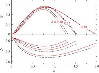
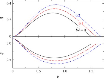
Reference Zhou, Peng, Zhang and Zhuge2014), as shown in figure 2. The profiles of growth rate
 $\unicode[STIX]{x1D714}_{i}$
and phase speed
 $c_{r}=\unicode[STIX]{x1D714}_{r}/k$
are cut off at the neutral wavenumber
 $k_{n}$
. It shows reassuring agreement with a particularly good capture of the growth rates. Though the wave speeds cannot be well captured by the Shkadov-type model, it can be improved by applying the method of weighted residuals, as discussed in Sisoev et al. (Reference Sisoev, Matar, Craster and Kumar2010). In this paper, however, we still use Shkadov-type equations for their simplicity and capability of capturing the flow characteristics.
Growth rate
 $\unicode[STIX]{x1D714}_{i}$
and phase speed
 $c_{r}$
versus wavenumber
 $k$
with
 $\unicode[STIX]{x1D6FF}$
as a parameter, for the flow of
 $\unicode[STIX]{x1D700}_{0}=0.05$
,
 $\widehat{\unicode[STIX]{x1D6FC}}=0.68$
,
 $T_{z}=5$
,
 $\unicode[STIX]{x1D6FD}=5$
and
 $\widehat{De}=0.05$
. Solid lines are given by linearized Shkadov-type modelling equations (3.2); dashed lines are given by the linearized full Navier–Stokes equations and full UCM constitutive equations. Both curves are cut off at the neutral wavenumber
 $k_{n}$
.

We first consider the influence of the tube flexibility on the system’s linear stability characteristics. The properties of the flexible tube are dominated by the damping coefficient
 $\widehat{\unicode[STIX]{x1D6FC}}$
, the longitudinal wall tension
 $T_{z}$
and the circumferential wall tension
 $\unicode[STIX]{x1D6FD}$
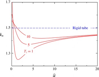
. Figure 3 illustrates the dependence of the neutral wavenumber
 $k_{n}$
on the damping coefficient
 $\widehat{\unicode[STIX]{x1D6FC}}$
. The longitudinal tension
 $T_{z}$
is considered as a parameter. It can be seen that the neutral wavenumber is non-monotonic as
 $\widehat{\unicode[STIX]{x1D6FC}}$
increases. This is similar to the results presented by Matar et al. (Reference Matar, Craster and Kumar2007) and Sisoev et al. (Reference Sisoev, Matar, Craster and Kumar2010). Physically, the wall damping plays a role in dissipating the system energy. In the case with small
 $\widehat{\unicode[STIX]{x1D6FC}}$
, the dissipation of the system would be intensified as
 $\widehat{\unicode[STIX]{x1D6FC}}$
increased. Thus, the neutral wavenumber decreases. When
 $\widehat{\unicode[STIX]{x1D6FC}}$
tends to infinity, the tube tends to become rigid. The dissipation effect is then weakened, and the neutral wavenumber increases. The dependence of the neutral wavenumber
 $k_{n}$
on
 $\unicode[STIX]{x1D6FD}$
with
 $\widehat{\unicode[STIX]{x1D6FC}}$
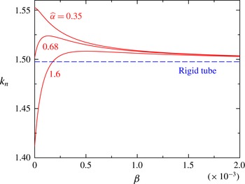
being a parameter is illustrated in figure 4. The stability of the annular falling film is influenced by the combination of the damping effect and the wall tension effect. In the first instance, when
 $\widehat{\unicode[STIX]{x1D6FC}}$
is small, the wall tension effect is dominant. Then as the wall tension increases, a smaller deformation of the tube wall would lead to a more stable system. The neutral wavenumber decreases monotonically as
 $\unicode[STIX]{x1D6FD}$
increases. In the second instance, when
 $\widehat{\unicode[STIX]{x1D6FC}}$
is relatively large, the damping effect is dominant. As the wall tension increases, a smaller deformation actually weakens the dissipation effect. As a result, the neutral wavenumber is increased. When the wall tension tends to infinity, the flexible tube will be expected to become a rigid one. Thus, the corresponding results tend to those of a rigid tube as illustrated in figures 3 and 4. In order to clarify the influences of the tube flexibility on the stability, we summarize the results in the following (
 ${\nearrow}$
means increasing,
 ${\searrow}$
means decreasing,
 ${\nearrow}{\searrow}$
means first increasing then decreasing, and
 ${\searrow}{\nearrow}$
means first decreasing then increasing):
 $$\begin{eqnarray}\displaystyle \left.\begin{array}{@{}c@{}}\widehat{\unicode[STIX]{x1D6FC}}{\nearrow}\Longrightarrow k_{n}{\searrow}{\nearrow}\text{for any }T_{z}\text{ or }\unicode[STIX]{x1D6FD},\\ T_{z}\text{ or }\unicode[STIX]{x1D6FD}{\nearrow}\Longrightarrow \left\{\begin{array}{@{}ll@{}}k_{n}{\searrow}\quad & \text{for small }\widehat{\unicode[STIX]{x1D6FC}},\\ k_{n}{\nearrow}{\searrow}\quad & \text{for large }\widehat{\unicode[STIX]{x1D6FC}}.\end{array}\right.\end{array}\right\} & & \displaystyle\end{eqnarray}$$
The neutral wavenumber
 $k_{n}$
versus the wall’s damping coefficient
 $\widehat{\unicode[STIX]{x1D6FC}}$
with the longitudinal tension as a parameter, for the flow of
 $\unicode[STIX]{x1D700}_{0}=0.05$
,
 $\unicode[STIX]{x1D6FF}=0.15$
and
 $\unicode[STIX]{x1D6FD}=5$
.

The neutral wavenumber
 $k_{n}$
versus the wall’s circumferential tension coefficient
 $\unicode[STIX]{x1D6FD}$
with damping coefficient
 $\widehat{\unicode[STIX]{x1D6FC}}$
as a parameter, for the flow of
 $\unicode[STIX]{x1D700}_{0}=0.05$
,
 $\widehat{\unicode[STIX]{x1D6FC}}=0.68$
and
 $T_{z}=5$
.

Growth rate
 $\unicode[STIX]{x1D714}_{i}$
and phase speed
 $c_{r}$
versus wavenumber
 $k$
with
 $\widehat{De}$
as a parameter, for the flow of
 $\unicode[STIX]{x1D700}_{0}=0.05$
,
 $\unicode[STIX]{x1D6FF}=0.15$
,
 $\widehat{\unicode[STIX]{x1D6FC}}=0.68$
,
 $T_{z}=5$
and
 $\unicode[STIX]{x1D6FD}=5$
. Both curves are cut off at the neutral wavenumber
 $k_{n}$
.

The dispersion curves for various Deborah numbers are shown in figure 5. It shows that the maximum growth rate and neutral wavenumber increase with increasing
 $\widehat{De}$
. The phase speed corresponding to each
 $k$
decreases. For simplicity, we consider the falling viscoelastic liquid film down a rigid tube. When
 $\unicode[STIX]{x1D700}_{0}\rightarrow 0$
, the dispersion relation corresponding to the planar limit can be derived as follows:
 $$\begin{eqnarray}\displaystyle & \displaystyle k_{n}^{2}=3(\widehat{We}+3\widehat{De}/\widehat{Re})+{\textstyle \frac{3}{10}}(9\widehat{We}+35\widehat{De}/\widehat{Re})\unicode[STIX]{x1D700}_{0}+O(\unicode[STIX]{x1D700}_{0}^{2}), & \displaystyle\end{eqnarray}$$
 $$\begin{eqnarray}\displaystyle & \displaystyle c_{r,n}=\unicode[STIX]{x1D714}_{r,n}/k_{n}=3+2\unicode[STIX]{x1D700}_{0}+{\textstyle \frac{13}{10}}\unicode[STIX]{x1D700}_{0}^{2}+O(\unicode[STIX]{x1D700}_{0}^{3}). & \displaystyle\end{eqnarray}$$
 $c_{r,n}$
means the phase speed at the neutral wavenumber. It can be seen that the neutral wavenumber
 $k_{n}$
will increase with increasing
 $\widehat{De}$
. However, the corresponding phase speed
 $c_{r,n}$
is independent of
 $\widehat{De}$
. This can be extended to the annular falling flow of the viscoelastic liquid film down the flexible tube, qualitatively. In figure 5, the differences in
 $c_{r,n}$
for various
 $\widehat{De}$
are very small. Furthermore, it can be found that the interval of the phase speed is extended with increasing
 $\widehat{De}$
. As a result, we may conclude that the fluid viscoelasticity destabilizes the film flow and strengthens the dispersion effect.
4 Steady travelling waves
4.1 Modelling and methodology
In this section, we consider travelling wave solutions of (2.23), (2.26) and (2.30) in the form of
 $q(\unicode[STIX]{x1D709})$
,
 $\unicode[STIX]{x1D702}(\unicode[STIX]{x1D709})$
and
 $\unicode[STIX]{x1D701}(\unicode[STIX]{x1D709})$
. Here
 $\unicode[STIX]{x1D709}=z-ct$
and
 $c$
is the velocity of the travelling wave. Integration of the continuity equation (2.23) with respect to
 $\unicode[STIX]{x1D709}$
gives
 $$\begin{eqnarray}q=q_{0}+{\textstyle \frac{1}{2}}c(\unicode[STIX]{x1D702}^{2}-\unicode[STIX]{x1D701}^{2}).\end{eqnarray}$$
Here,
 $q_{0}$
is an integration constant, which is expressed as
 $q_{0}=\int _{\unicode[STIX]{x1D701}}^{\unicode[STIX]{x1D702}}r(V_{z}-c)\,\text{d}r$
. Physically, it represents the volume flow rate of the falling film at the reference frame moving with the wave speed. Then, equation (2.26) can be rewritten as
 $$\begin{eqnarray}\displaystyle -cq^{\prime }+MM^{\prime } & = & \displaystyle h\unicode[STIX]{x1D702}\left(1-\frac{\unicode[STIX]{x1D700}}{2}\right)\left[\frac{1}{\unicode[STIX]{x1D711}(\unicode[STIX]{x1D700}_{0})\widehat{Re}}-\frac{1}{\widehat{We}}\left(\unicode[STIX]{x1D701}^{\prime \prime \prime }+\frac{1}{\unicode[STIX]{x1D705}^{2}\unicode[STIX]{x1D701}^{2}}\unicode[STIX]{x1D701}^{\prime }\right)\right]\nonumber\\ \displaystyle & & \displaystyle -\,\frac{L}{\unicode[STIX]{x1D711}(\unicode[STIX]{x1D700}_{0})\widehat{Re}}+\frac{\widehat{De}}{\unicode[STIX]{x1D711}(\unicode[STIX]{x1D700}_{0})\widehat{Re}}(-cLL^{\prime }-cJ\unicode[STIX]{x1D702}^{\prime }+NN^{\prime }).\end{eqnarray}$$
Here,
 $(\boldsymbol{\cdot })^{\prime }$
denotes the derivative of
 $(\boldsymbol{\cdot })$
with respect to
 $\unicode[STIX]{x1D709}$
, and the expressions of
 $M^{\prime }$
,
 $L^{\prime }$
and
 $N^{\prime }$
are given in appendix C. Similarly, equation (2.30) can be rewritten as follows:
 $$\begin{eqnarray}-c\widehat{\unicode[STIX]{x1D6FC}}\unicode[STIX]{x1D702}^{\prime }=T_{z}\unicode[STIX]{x1D702}^{\prime \prime }-\frac{1}{\unicode[STIX]{x1D705}^{2}}T_{0}\left(\frac{1}{\unicode[STIX]{x1D702}}-\frac{1}{b}\right)-\frac{1}{\unicode[STIX]{x1D705}^{2}}\unicode[STIX]{x1D6FD}\frac{\unicode[STIX]{x1D702}-b}{\unicode[STIX]{x1D702}^{2}}+\unicode[STIX]{x1D701}^{\prime \prime }+\frac{1}{\unicode[STIX]{x1D705}^{2}}\left(\frac{1}{a}-\frac{1}{\unicode[STIX]{x1D701}}\right).\end{eqnarray}$$
We now seek the solutions with period
 $l=2\unicode[STIX]{x03C0}/s$
under the phase condition
 $\unicode[STIX]{x1D701}(0)=a$
and the integral condition as follows:
 $$\begin{eqnarray}\frac{s}{2\unicode[STIX]{x03C0}}\int _{0}^{2\unicode[STIX]{x03C0}/s}\unicode[STIX]{x1D702}\,\text{d}\unicode[STIX]{x1D709}=b.\end{eqnarray}$$
In this study, equations (4.1)–(4.3) are discretized by the Fourier spectral method, where the pseudo-spectral method is adopted for the nonlinear term. The nonlinear algebraic system with one parameter
 $s$
is solved by using the Newton–Kantorovich method and the continuation method.
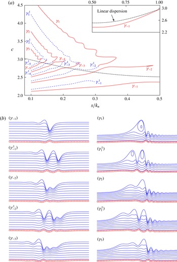
(a) Dependence of the velocities of the steady travelling waves on the normalized frequency, for
 $\unicode[STIX]{x1D700}_{0}=0.05$
,
 $\unicode[STIX]{x1D6FF}=0.15$
,
 $\widehat{\unicode[STIX]{x1D6FC}}=0.68$
,
 $T_{z}=5$
,
 $\unicode[STIX]{x1D6FD}=5$
and
 $\widehat{De}=0.05$
. Solid lines denote the
 $\unicode[STIX]{x1D6FE}_{\pm i}$
families, dashed lines denote the
 $\unicode[STIX]{x1D6FE}_{\pm i}^{1}$
families, and the dash-dotted line denotes the linear dispersion curve (
 $c_{r}$
–
 $k$
curve in linear stability). (b) Corresponding wave patterns of the gas–liquid interface and liquid–wall interface for
 $\unicode[STIX]{x1D6FE}_{\pm i}$
and
 $\unicode[STIX]{x1D6FE}_{\pm i}^{1}$
travelling waves (
 $s/k_{n}=0.1$
). The streamlines are observed in convected coordinates.

It is worth pointing out that there exist multiple solutions for a single value of
 $s$
, and the bifurcation structures of the solutions are very complex. To distinguish various solution families, notations
 $\unicode[STIX]{x1D6FE}_{\pm i}$
and
 $\unicode[STIX]{x1D6FE}_{\pm i}^{j}$
are introduced, where
 $\unicode[STIX]{x1D6FE}_{\pm i}$
denotes the travelling wave solution with one hump (one hollow) following many capillary waves. The one-hump (one-hollow) solution is constructed by
 $i$
sub-humps (sub-hollows), and the sign is positive (negative) for the fast (slow) wave family;
 $\unicode[STIX]{x1D6FE}_{\pm i}^{j}$
denotes the travelling wave pattern with
 $j$
humps between the one-hump and capillary waves.
Considering the complexity of the solution, we only give the
 $\unicode[STIX]{x1D6FE}_{\pm i}$
and
 $\unicode[STIX]{x1D6FE}_{\pm i}^{1}$
families in figure 6(a), and corresponding wave patterns are shown in figure 6(b). In order to show the wave patterns in a simpler way, a new coordinate system is introduced, which is based on the following transformation:
 $$\begin{eqnarray}r=b-y,\quad z=x.\end{eqnarray}$$
In the new coordinates
 $(x,y)$
, we denote the location of the liquid–wall interface by
 $\unicode[STIX]{x1D712}$
; then the location of the free surface is
 $\unicode[STIX]{x1D712}+h$
.
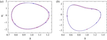
Phase trajectories illustrating a flip, which corresponds to a bifurcation of a stable limit cycle of period
 $T$
into a stable limit cycle of period
 $2T$
. The solid line is a stable limit cycle of period
 $2\unicode[STIX]{x03C0}/s_{1}$
before the flip bifurcation; the dashed line is a stable limit cycle of period
 $2\unicode[STIX]{x03C0}/s_{2}$
after the flip bifurcation. (a) The
 $\unicode[STIX]{x1D6FE}_{-2}$
family bifurcates by a flip from the
 $\unicode[STIX]{x1D6FE}_{-1}$
family with
 $s_{1}=1.3918$
and
 $s_{2}=0.6960$
. (b) The
 $\unicode[STIX]{x1D6FE}_{-1}^{1}$
family bifurcates by a flip from the
 $\unicode[STIX]{x1D6FE}_{-1}$
family with
 $s_{1}=0.9092$
and
 $s_{2}=0.4543$
.

The phase trajectories of these wave patterns have been discussed comprehensively by Chang & Demekhin (Reference Chang and Demekhin2002). In figure 6(a), the slow family
 $\unicode[STIX]{x1D6FE}_{-1}$
branches off the trivial solution at the cutoff wavenumber
 $s=k_{n}$
corresponding to the Hopf bifurcation point, which is a stable limit cycle in the
 $(h,h^{\prime })$
plane. The wave in this family has a speed that is less than that of a spatially amplified infinitesimal wave at the same frequency. Moreover, both the
 $\unicode[STIX]{x1D6FE}_{-2}$
and
 $\unicode[STIX]{x1D6FE}_{-1}^{1}$
families bifurcate by flipping (period doubling) from the same family
 $\unicode[STIX]{x1D6FE}_{-1}$
at different wavenumbers. Thus, the stable limit cycle in the
 $(h,h^{\prime })$
plane becomes only slightly different, as illustrated in figure 7. The key feature is that the period of the limit cycle doubles through the bifurcation (Dercole & Rinaldi Reference Dercole and Rinaldi2011). Generally, the bifurcation diagram is similar to those presented by Shkadov & Sisoev (Reference Shkadov and Sisoev2004). However, the presence of the tube flexibility and the fluid viscoelasticity tends to induce some differences. For instance, the fluid viscoelasticity will accelerate the fast family waves, but decelerate the slow family waves. In other words, the fluid viscoelasticity will intensify the dispersion effect. Detailed analysis and physical explanation will be given in the following. Chang (Reference Chang1994)’s stability analysis showed that the most stable waves lie on the primary slow family
 $\unicode[STIX]{x1D6FE}_{-1}$
and fast family
 $\unicode[STIX]{x1D6FE}_{1}$
. Thus, we mainly consider these two primary families in the following.
4.2 The effect of surface tension and fluid viscoelasticity
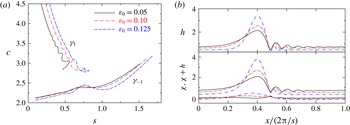
(a) Dependence of the velocities of two primary travelling waves on the normalized frequency, and (b) corresponding profiles of thickness and two interfaces of the
 $\unicode[STIX]{x1D6FE}_{1}$
family at
 $s=0.2$
, for the flow of
 $\unicode[STIX]{x1D6FF}=0.15$
,
 $\widehat{\unicode[STIX]{x1D6FC}}=0.68$
,
 $T_{z}=5$
,
 $\unicode[STIX]{x1D6FD}=5$
,
 $\widehat{De}=0$
and various initial relative thicknesses
 $\unicode[STIX]{x1D700}_{0}$
.

We first consider the effect of circumferential surface tension, which is inversely proportional to the tube radius (
 $b=1/\unicode[STIX]{x1D700}_{0}$
). Figure 8 shows the bifurcation diagram (only the primary slow and fast families being considered) and the corresponding interfacial profiles (both free surface and liquid–wall interface) of the primary fast family under different
 $\unicode[STIX]{x1D700}_{0}$
. From figure 8(a), it can be seen that the wave speed of the primary slow family decreases with increasing
 $\unicode[STIX]{x1D700}_{0}$
. However, the wave speed of the primary fast family is promoted. This may suggest that the relative thickness acts to strengthen the dispersion of the system. This is different from the situation of the annular film flowing down the outer surface of a cylinder (Sisoev et al.
Reference Sisoev, Craster, Matar and Gerasimov2006). Physically, in that situation, the circumferential surface tension acts to pull the free surface down towards the cylinder wall. The circumferential surface tension plays a role in decreasing the wave amplitude
 $h_{max}$
of the primary fast family wave. As a result, the wave speed becomes smaller than that in the planar film flow. However, in this study, the circumferential surface tension acts to pull the free surface towards the tube axis, or plays a role in strengthening the wave amplitude
 $h_{max}$
. Thus, the wave speed would be larger than that in the planar case. Furthermore, the circumferential surface tension would make the flexible tube shrink, when the tube radius is small enough (e.g.
 $\unicode[STIX]{x1D700}_{0}=0.1$
in figure 8
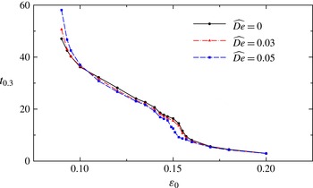
b). It can be found that the tube wall would undergo a larger deformation if the radius was smaller. This may be attributed to the larger circumferential surface tension effect. It is worth noting that tube closure would happen when
 $\unicode[STIX]{x1D700}$
is larger than the critical value
 $\unicode[STIX]{x1D700}_{c}$
. Then, the steady travelling waves cannot be identified. The critical value
 $\unicode[STIX]{x1D700}_{c}$
depends closely on both the film viscoelasticity and the tube flexibility.
(a) Dependence of the velocities of two primary travelling waves on the normalized frequency, and (b) corresponding profiles of thickness and two interfaces for the
 $\unicode[STIX]{x1D6FE}_{1}$
family at
 $s=0.2$
, for the flow of
 $\unicode[STIX]{x1D700}_{0}=0.05$
,
 $\unicode[STIX]{x1D6FF}=0.15$
,
 $\widehat{\unicode[STIX]{x1D6FC}}=0.68$
,
 $T_{z}=5$
,
 $\unicode[STIX]{x1D6FD}=5$
and various
 $\widehat{De}$
.

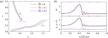
The effect of fluid viscoelasticity on steady travelling waves is shown in figure 9. As shown in figure 9(a), the fluid viscoelasticity plays a role in boosting the wave speed of the primary fast family, but delays that of the primary slow family. This is consistent with the linear stability analysis, in which the viscoelastic effect acts to strengthen the wave dispersion. In figure 9(b), it is shown that the fluid viscoelasticity acts to weaken the capillary ripples. This may be attributed to the fact that near the wave troughs the velocity gradients (and hence shearing strains) are relatively large. Then, the polymeric molecules experience strong stretching around the troughs, which results in thinner capillary ripples. As a result, the amplitude of the main hump
 $h_{max}$
increases due to the conservation of mass.
4.3 The effect of tube flexibility
(a) Dependence of the velocities of two primary travelling waves on the normalized frequency, and (b) corresponding profiles of thickness and two interfaces for the
 $\unicode[STIX]{x1D6FE}_{1}$
family at
 $s=0.2$
, for the flow of
 $\unicode[STIX]{x1D700}_{0}=0.05$
,
 $\unicode[STIX]{x1D6FF}=0.15$
,
 $T_{z}=5$
,
 $\unicode[STIX]{x1D6FD}=5$
,
 $\widehat{De}=0$
and various
 $\widehat{\unicode[STIX]{x1D6FC}}$
.

The effects of the damping coefficient
 $\widehat{\unicode[STIX]{x1D6FC}}$
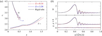
on the flow characteristics are shown in figure 10. As illustrated in figure 10(a), the wave speed of the primary slow family
 $\unicode[STIX]{x1D6FE}_{-1}$
first increases and then decreases with increasing
 $\widehat{\unicode[STIX]{x1D6FC}}$
. The variation of the neutral wavenumber is also non-monotonic. For the primary fast family
 $\unicode[STIX]{x1D6FE}_{1}$
, the amplitudes of the swing of
 $c$
–
 $s$
curves first decrease and then increase. Moreover, the results indicate that the variation of
 $\widehat{\unicode[STIX]{x1D6FC}}$
has little influence on the wave patterns of the
 $\unicode[STIX]{x1D6FE}_{-1}$
family, but has a distinctive influence on those of the
 $\unicode[STIX]{x1D6FE}_{1}$
family. The wave patterns of the
 $\unicode[STIX]{x1D6FE}_{1}$
family for various
 $\widehat{\unicode[STIX]{x1D6FC}}$
are shown in figure 10(b). As
 $\widehat{\unicode[STIX]{x1D6FC}}$
increases, the wall displacement of the flexible tube is decreased. The amplitudes of the capillary waves first decrease and then increase. This is also consistent with the linear stability analysis in § 3. Since the capillary waves are depressed with the increasing of
 $\widehat{\unicode[STIX]{x1D6FC}}$
, the amplitude of the main hump will increase due to the conservation of mass. However, when
 $\widehat{\unicode[STIX]{x1D6FC}}$
increases to a large value, the displacements of the tube wall are very small. The flexible tube tends to approach a rigid one. Then, the dissipation effect is actually weakened. As a result, the capillary waves have a larger amplitude compared to the situation with a moderate damping coefficient.
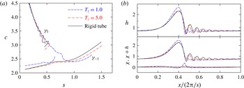
The bifurcation diagrams for various
 $T_{z}$
are shown in figure 11(a). When
 $\widehat{\unicode[STIX]{x1D6FC}}$
,
 $T_{z}$
and
 $\unicode[STIX]{x1D6FD}$
are at small values, the branch of travelling waves bifurcating from
 $s=k_{n}$
is connected to the primary fast family
 $\unicode[STIX]{x1D6FE}_{1}$
as
 $s$
decreases from
 $k_{n}$
(e.g.
 $T_{z}=1.0$
). As
 $T_{z}$
increases, the situation is reversed (e.g.
 $T_{z}=5.0$
) and the branch is connected to the primary slow family
 $\unicode[STIX]{x1D6FE}_{-1}$
. Mathematically, the two branches would collide when
 $T_{z}$
equals some critical value, and the connection between them would be exchanged due to the effect of flexibility. A similar phenomenon was also observed due to the effect of viscous dispersion (Salamon, Armstrong & Brown Reference Salamon, Armstrong and Brown1994). Besides, as
 $T_{z}$
increases, the speeds of waves with wavenumbers just branching off the trivial solution (e.g.
 $1<s<k_{n}$
) increase monotonically. For the fast family, the increasing of
 $T_{z}$
makes the
 $c$
–
 $s$
curve more swinging. As illustrated in figure 11(b), the deformation of the flexible tube decreases, and the capillary waves on the film free surface are stimulated when the wall tension
 $T_{z}$
increases. Physically, the increasing of
 $T_{z}$
makes the flexible tube stiffer. Corresponding smaller deformations of the tube wall may weaken the damping effect. Then, the amplitudes of the capillary waves are enlarged. The result also shows that the effect of
 $\unicode[STIX]{x1D6FD}$
on the travelling waves is similar to that of
 $T_{z}$
, since the increasing of
 $T_{z}$
or
 $\unicode[STIX]{x1D6FD}$
would enhance the stiffness of the flexible tube.
(a) Dependence of the velocities of two primary travelling waves on the normalized frequency, and (b) corresponding profiles of thickness and two interfaces for the
 $\unicode[STIX]{x1D6FE}_{1}$
family at
 $s=0.2$
, for the flow of
 $\unicode[STIX]{x1D700}_{0}=0.05$
,
 $\unicode[STIX]{x1D6FF}=0.15$
,
 $\widehat{\unicode[STIX]{x1D6FC}}=0.68$
,
 $\unicode[STIX]{x1D6FD}=5$
,
 $\widehat{De}=0$
and various
 $T_{z}$
.

5 Transient numerical solutions
In this section, the evolution of the initial wave packet is obtained by solving equations (2.23), (2.26) and (2.30) numerically. A sixth-order compact finite-difference scheme is adopted for spatial derivatives with space interval
 $\unicode[STIX]{x0394}z=0.05$
. A fourth-order Runge–Kutta scheme is used for the temporal integral with time interval
 $\unicode[STIX]{x0394}t=10^{-4}$
. The initial condition is (recall that
 $b=1/\unicode[STIX]{x1D700}_{0}$
)
 $$\begin{eqnarray}h(z,0)=1.0+0.05\times \exp [-(z-30.0)^{2}],\quad \unicode[STIX]{x1D702}(z,0)=b,\quad q(z,0)=b.\end{eqnarray}$$
The locations of the two interfaces, and the flow rate at the inlet (
 $z=0.0$
), are assumed to be fixed with
 $h(0,t)=1.0$
,
 $\unicode[STIX]{x1D702}(0,t)=b$
,
 $q(0,t)=b$
. At the outlet (
 $z=1200$
), an absorbing boundary condition (Hu Reference Hu1996) is imposed in order to minimize the upstream feedback. A perfectly matched layer, which can absorb the outgoing waves, is defined in a region next to the artificial boundary. In this layer, linearized equations are used to numerically calculate the eigenvalues and eigenvectors. Then, the outgoing waves can be determined. The evolution of the film thickness,
 $h$
, is illustrated in figure 12. At first, the perturbation in
 $h$
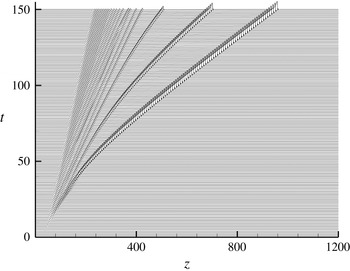
forms a wave packet, which is transported downstream by the mean flow. After that, it disperses into several capillary waves. The front wave quickly evolves into a solitary-like waveform. It separates from the wave packet and propagates rapidly downstream. However, at the rear of the wave structure, capillary waves with small amplitudes are preserved.
Evolution of film thickness (
 $h=\unicode[STIX]{x1D702}-\unicode[STIX]{x1D701}$
) over time, for the flow of
 $\unicode[STIX]{x1D700}_{0}=0.05$
,
 $\unicode[STIX]{x1D6FF}=0.15$
,
 $\widehat{\unicode[STIX]{x1D6FC}}=3.39$
,
 $T_{z}=1$
,
 $\unicode[STIX]{x1D6FD}=5$
and
 $\widehat{De}=0.05$
.

(a) Profiles of the free surface and the liquid–wall interface at
 $t=150.0$
for the flow of
 $\unicode[STIX]{x1D700}_{0}=0.01$
,
 $\unicode[STIX]{x1D6FF}=0.15$
,
 $\widehat{\unicode[STIX]{x1D6FC}}=0.68$
,
 $T_{z}=1$
and
 $\unicode[STIX]{x1D6FD}=5$
, and (b) corresponding solitary-like wave in three-dimensional display.

(a) Profiles of the free surface and the liquid–wall interface at
 $t=150.0$
for the flow of
 $\unicode[STIX]{x1D700}_{0}=0.08$
,
 $\unicode[STIX]{x1D6FF}=0.15$
,
 $\widehat{\unicode[STIX]{x1D6FC}}=3.39$
,
 $T_{z}=1$
and
 $\unicode[STIX]{x1D6FD}=5$
, and (b) corresponding solitary-like wave in three-dimensional display, in which the shrinking of the tube can be seen clearly.

Profiles of the free surface and the liquid–wall interface at
 $t=150.0$
, for the flow of
 $\unicode[STIX]{x1D700}_{0}=0.05$
,
 $\unicode[STIX]{x1D6FF}=0.15$
,
 $\widehat{\unicode[STIX]{x1D6FC}}=3.39$
,
 $T_{z}=1$
,
 $\unicode[STIX]{x1D6FD}=5$
and various
 $\widehat{De}$
.

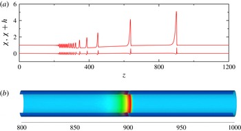
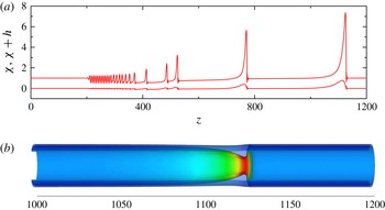
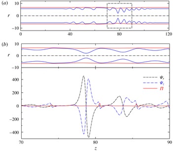
Though the evolution of the film thickness is similar to that of falling film on a flexible plane, which is considered by Sisoev et al. (Reference Sisoev, Matar, Craster and Kumar2010) and Peng et al. (Reference Peng, Zhang and Zhuge2014), the displacement of the flexible wall is distinctly different. For the planar film flow, it can be seen that the flexible wall deforms away from the fluid film at the crest (where
 $\unicode[STIX]{x1D701}_{z,z}>0$
). It is pushed by a pressure difference caused by the surface tension in a streamwise (
 $z$
) direction, mathematically
 $\unicode[STIX]{x1D701}_{z,z}/\widehat{We}$
in equation (2.19). However, in this study, the pressure difference caused by the surface tension in the circumferential direction will pull the tube towards the core while
 $\unicode[STIX]{x1D701}<a$
and reverse while
 $\unicode[STIX]{x1D701}>a$
, mathematically
 $\unicode[STIX]{x1D705}^{-2}(a^{-1}-\unicode[STIX]{x1D701}^{-1})/\widehat{We}$
in equation (2.19). Generally, we have
 $\unicode[STIX]{x1D701}_{z,z}>0$
and
 $\unicode[STIX]{x1D701}<a$
at the crest of a solitary-like wave. Thus, the displacement of the flexible tube depends on the competition between the effects of longitudinal and circumferential surface tensions. If the initial tube radius,
 $b$
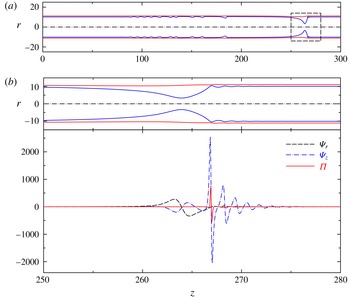
, is relatively large, the circumferential surface tension effect is weak and the flexible tube will expand at the crest, as illustrated in figure 13. This is similar to what occurs in the planar case. However, if
 $b$
is relatively small, the circumferential surface tension effect becomes strong, and the flexible tube will shrink at the crest, as illustrated in figure 14. Comparing figures 13 and 14, it can be found that the maximum thickness and the speed of the front solitary-like wave are both increased with increasing
 $\unicode[STIX]{x1D700}_{0}$
. But the speed of the rear wave is decreased. We may conclude that
 $\unicode[STIX]{x1D700}_{0}$
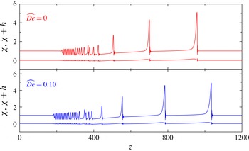
acts to enhance the dispersion of the system, which is consistent with the bifurcation analysis in § 4.2. The fluid viscoelasticity also has substantial effects on the evolution of the annular falling film. Figure 15 shows the profiles of the free surface and liquid–wall interface at
 $t=150.0$
for both a Newtonian fluid and a weak viscoelastic fluid. It can be found that the front solitary-like wave of the viscoelastic film propagates much faster than that of the Newtonian fluid. However, the rear wave of the viscoelastic film propagates much more slowly. In other words, the fluid viscoelasticity promotes the dispersion of the system, which is also consistent with the bifurcation analysis in § 4.2.
Minimum radius of the free surface versus time for a Newtonian fluid and a weak viscoelastic fluid (
 $\widehat{De}=0.03$
) under various initial relative thickness
 $\unicode[STIX]{x1D700}_{0}$
, for the flow of
 $\unicode[STIX]{x1D6FF}=0.15$
,
 $\widehat{\unicode[STIX]{x1D6FC}}=3.39$
,
 $T_{z}=1$
and
 $\unicode[STIX]{x1D6FD}=5$
.

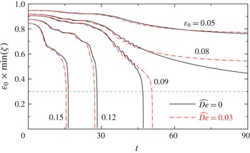
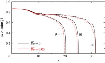
When the radius of the flexible tube is small enough, an interesting phenomenon called tube closure will occur. Figure 16 gives the evolution of the minimum radius of the free surface for a Newtonian fluid and a weak viscoelastic fluid. According to equation (5.1a–c
), the initial minimum radius of the free surface is
 $\min (\unicode[STIX]{x1D701}(z,0))=b-\max (h(z,0))=1/\unicode[STIX]{x1D700}_{0}-(1+0.05)$
. Then we have
 $\unicode[STIX]{x1D700}_{0}\min (\unicode[STIX]{x1D701}_{0})=1-1.05\unicode[STIX]{x1D700}_{0}$
as the initial value in this figure. When
 $\unicode[STIX]{x1D700}_{0}\leqslant 0.08$
, the minimum radius of the free surface is limited to a finite value. Thus tube closure cannot occur. However, when
 $\unicode[STIX]{x1D700}_{0}\geqslant 0.09$
, the minimum radius of the free surface decreases until tube closure happens. It can be concluded that the critical relative thickness
 $\unicode[STIX]{x1D700}_{c}$
is located between
 $0.08$
and
 $0.09$
. The critical value
 $\unicode[STIX]{x1D700}_{c}$
depends closely on both the film viscoelasticity and the tube flexibility. In this study, we choose the time when
 $\unicode[STIX]{x1D700}_{0}\min (\unicode[STIX]{x1D701})=0.3$
, denoted by
 $t_{0.3}$
, as an approximate closure time. It is reasonable since the minimum core radius decreases rapidly when
 $\unicode[STIX]{x1D700}_{0}\min (\unicode[STIX]{x1D701})<0.3$
. Besides, the long-wavelength assumption and the axial velocity profile assumption may not be accurate enough in the situation with thick film. Similar criteria for tube closure can also be found in previous literature (Halpern & Grotberg Reference Halpern and Grotberg1993; Halpern et al.
Reference Halpern, Fujioka and Grotberg2010).
Approximate closure time
 $t_{0.3}$
versus
 $\unicode[STIX]{x1D700}_{0}$
under various
 $\widehat{De}$
, for the flow of
 $\unicode[STIX]{x1D6FF}=0.15$
,
 $\widehat{\unicode[STIX]{x1D6FC}}=3.39$
,
 $T_{z}=1$
and
 $\unicode[STIX]{x1D6FD}=5$
.

(a) Profiles of two interfaces at
 $t=50.66$
just before tube closure happens, when
 $\unicode[STIX]{x1D700}_{0}\min (\unicode[STIX]{x1D701})=0.3$
, and (b) profiles of the surface tension and viscoelasticity terms in equation (2.29) for the weak viscoelastic fluid (
 $\widehat{De}=0.03$
) flow of
 $\unicode[STIX]{x1D700}_{0}=0.09$
,
 $\unicode[STIX]{x1D6FF}=0.15$
,
 $\widehat{\unicode[STIX]{x1D6FC}}=3.39$
,
 $T_{z}=1$
and
 $\unicode[STIX]{x1D6FD}=5$
.

(a) Profiles of two interfaces at
 $t=15.51$
just before tube closure happens, when
 $\unicode[STIX]{x1D700}_{0}\min (\unicode[STIX]{x1D701})=0.3$
, and (b) distributions of the two surface tension terms and viscoelasticity term in equation (2.29) for the weak viscoelastic fluid (
 $\widehat{De}=0.03$
) flow of
 $\unicode[STIX]{x1D700}_{0}=0.15$
,
 $\unicode[STIX]{x1D6FF}=0.15$
,
 $\widehat{\unicode[STIX]{x1D6FC}}=3.39$
,
 $T_{z}=1$
and
 $\unicode[STIX]{x1D6FD}=5$
.

Figure 17 shows the approximate closure times under various
 $\unicode[STIX]{x1D700}_{0}$
for Newtonian and weak viscoelastic fluids. It can be found that the fluid viscoelasticity boosts the tube closure process when
 $\unicode[STIX]{x1D700}_{0}$
is relatively large, e.g.
 $\unicode[STIX]{x1D700}_{0}>0.1$
, but prolongs the closure time when
 $\unicode[STIX]{x1D700}_{0}$
is relatively small. Two typical cases are investigated in detail to illustrate this interesting phenomenon. Figure 18 shows the profiles of the free surface and tube wall at
 $t=t_{0.3}$
for relatively small
 $\unicode[STIX]{x1D700}_{0}=0.09$
. Corresponding distributions of
 $\unicode[STIX]{x1D6F1}$
,
 $\unicode[STIX]{x1D6F9}_{z}$
and
 $\unicode[STIX]{x1D6F9}_{r}$
along the
 $z$
-axis are also presented. As we have mentioned in equation (2.29),
 $\unicode[STIX]{x1D6F1}$
indicates the contribution of fluid viscoelasticity, while
 $\unicode[STIX]{x1D6F9}_{z}$
and
 $\unicode[STIX]{x1D6F9}_{r}$
represent the contributions of longitudinal and circumferential surface tension effects, respectively. Similar results at
 $t=t_{0.3}$
for relatively large
 $\unicode[STIX]{x1D700}_{0}=0.15$
are illustrated in figure 19. Inspecting these two figures shows that
 $\unicode[STIX]{x1D6F1}$
varies mainly around the wavefront of humps, where the film is very thin;
 $\unicode[STIX]{x1D6F1}$
changes from positive to negative along the positive
 $z$
-axis. According to equation (2.26), we know that the flux increases where
 $\unicode[STIX]{x1D6F1}>0$
and decreases where
 $\unicode[STIX]{x1D6F1}<0$
. Then, it can be deduced that the fluid viscoelasticity plays a role in increasing the thickness around the wavefront of humps. As a result of conservation of mass, the heights of the humps decrease. Here, the fluid viscoelasticity acts similarly to the longitudinal surface tension term
 $\unicode[STIX]{x1D6F9}_{z}$
, as Peng et al. (Reference Peng, Zhang and Zhuge2014) indicated. This is attributed to the presence of the normal stress difference of viscoelastic fluids. Therefore, the fluid viscoelasticity acts to prolong the closure time due to the normal stress. On the other hand, as has been noted, the fluid viscoelasticity also plays a role in promoting the system dispersion. It acts to accelerate the development of the front solitary-like wave. This may lead to earlier tube closure, when the initial thickness of annular films is relatively large.
Figures 18 and 19 also show the competition between the effects of longitudinal and circumferential surface tension (
 $\unicode[STIX]{x1D6F9}_{z}$
and
 $\unicode[STIX]{x1D6F9}_{r}$
), which can be a supplement to the discussion in the second paragraph of this section. It can be seen that the maximum or minimum value of
 $\unicode[STIX]{x1D6F9}_{r}$
mainly occurs at a position near to the humps. This indicates that the circumferential surface tension has a greater influence here. Moreover,
 $\unicode[STIX]{x1D6F9}_{r}$
is almost opposite in value distribution to
 $\unicode[STIX]{x1D6F9}_{z}$
. This means that the influence of the circumferential surface tension is distinctly different from that of the longitudinal surface tension. As the tube radius decreases, the maximum value of
 $\unicode[STIX]{x1D6F9}_{r}$
would be larger than the maximum value of
 $\unicode[STIX]{x1D6F9}_{z}$
. Then, the circumferential surface tension will play a more important role in the flow. In particular, while the tube radius is large, e.g.
 $\unicode[STIX]{x1D700}_{0}=0.09$
, the longitudinal surface tension effect is dominant and the annular film flow is mainly influenced by Kapitza instability; while the tube radius is small, e.g.
 $\unicode[STIX]{x1D700}_{0}=0.15$
, the circumferential surface tension is dominant and the annular film flow is mainly influenced by Plateau–Rayleigh instability. Actually, there is another way of comparing the two surface tension effects, which was introduced by Kalliadasis & Chang (Reference Kalliadasis and Chang1994) and developed by Duprat, Ruyer-Quil & Giorgiutti-Dauphiné (Reference Duprat, Ruyer-Quil and Giorgiutti-Dauphiné2009) and Ruyer-Quil & Kalliadasis (Reference Ruyer-Quil and Kalliadasis2012). Following their method, the capillary length can be estimated as
 $$\begin{eqnarray}l_{c}^{\ast }=\sqrt{\unicode[STIX]{x1D6FE}^{\ast }/(\unicode[STIX]{x1D70C}^{\ast }g^{\ast })}=\unicode[STIX]{x1D705}^{-3/2}H^{\ast }\sqrt{\unicode[STIX]{x1D711}(\unicode[STIX]{x1D700}_{0})\widehat{Re}/\widehat{We}}.\end{eqnarray}$$
Then, the ratio of the capillary length to the tube radius is
 $$\begin{eqnarray}l_{c}^{\ast }/R^{\ast }=\unicode[STIX]{x1D705}^{-3/2}\unicode[STIX]{x1D700}_{0}\sqrt{\unicode[STIX]{x1D711}(\unicode[STIX]{x1D700}_{0})\widehat{Re}/\widehat{We}}.\end{eqnarray}$$
Physically, this ratio measures the azimuthal curvature effect, which corresponds to the Plateau–Rayleigh instability. The higher the ratio, the stronger the azimuthal curvature effect. The ratios corresponding to figures 18 and 19 are 1.4842 and 2.4737, respectively. Therefore, the azimuthal curvature effect in figure 19 is stronger, which is consistent with the result obtained in the previous paragraph by comparing the values of
 $\unicode[STIX]{x1D6F9}_{z}$
and
 $\unicode[STIX]{x1D6F9}_{r}$
.
Minimum radius of the free surface versus time for a Newtonian fluid and a weak viscoelastic fluid (
 $\widehat{De}=0.03$
) under various wall circumferential tension coefficients
 $\unicode[STIX]{x1D6FD}$
, for the flow of
 $\unicode[STIX]{x1D700}_{0}=0.13$
,
 $\unicode[STIX]{x1D6FF}=0.15$
,
 $\widehat{\unicode[STIX]{x1D6FC}}=3.39$
and
 $T_{z}=1$
.

Figure 20 shows the evolution of the minimum radius of the free surface for a Newtonian fluid and a weak viscoelastic fluid under various tubes’ hoop elasticity
 $\unicode[STIX]{x1D6FD}$
. It can be seen that the closure time is prolonged with increasing
 $\unicode[STIX]{x1D6FD}$
. Conceivably, the shrinking of the tube would promote the emergence of tube closure. Therefore, the increasing of the tube stiffness is helpful in reducing the magnitude of deformation, and in preventing tube closure (Halpern & Grotberg Reference Halpern and Grotberg1992). The increasing of tube stiffness would also strengthen the capillary waves, and the amplitude of the main hump would decrease due to the conservation of mass. This is similar to the effect of the normal stresses of fluid viscoelasticity, and would also prolong the tube closure.
6 Conclusion
This investigation addresses the dynamics of annular viscoelastic films falling down the inner surface of a flexible tube. Based on the integral boundary layer theory, the profile of the axial velocity is assumed and the corresponding momentum equation is integrated. A set of nonlinear evolution equations is derived, which is valid for a weak viscoelastic film with moderate Reynolds number. Linear stability analysis of the model is performed, and is confirmed by comparing with the results obtained from the linearized full Navier–Stokes equations and UCM constitutive equations. The results indicate that the tube flexibility, which includes wall damping and tension, plays a dual role in the stability of the film flow. In the case where the wall tension effect is dominant, the wall tension acts to stabilize. However, when the damping effect is dominant, the wall tension tends to promote instability. Physically, this is attributed to the fact that the wall perturbation displacement becomes smaller with increasing wall tension. Therefore, the dissipation effect of wall damping is weakened.
In the nonlinear regime, the steady travelling waves are identified. Bifurcation analysis is performed to catalogue the various families of steady travelling waves. Corresponding wave patterns are also presented. According to the properties of the two primary families (fastest family
 $\unicode[STIX]{x1D6FE}_{1}$
and slowest family
 $\unicode[STIX]{x1D6FE}_{-1}$
), it can be concluded that the flexible tube tends to have larger deformation when the tube radius is smaller. The tube stiffness acts to stimulate capillary waves. However, the fluid viscoelasticity tends to weaken them and to strengthen the dispersion. Transient numerical solutions are also carried out to examine the evolution of the annular films. The results show that the deformation of the tube wall is distinct from that of a plane investigated by Sisoev et al. (Reference Sisoev, Matar, Craster and Kumar2010) and Peng et al. (Reference Peng, Zhang and Zhuge2014). The tube is pulled inward due to the pressure difference caused by the surface tension in the circumferential direction. As a result, tube closure may occur when its radius is small enough. The fluid viscoelasticity can also promote tube closure when the tube radius is relatively small, where viscoelasticity acts to boost the dispersion effect. However, it tends to postpone the closure in the case of a large tube radius due to the presence of normal stress differences. Moreover, the increasing of tube stiffness will prolong the tube closure.
In this study, the averaged set of equations is limited to describing the flow of the weak viscoelastic liquid thin film. Thus, it may have some shortcomings if we want to predict the tube closure process of strong viscoelastic fluids accurately. In the near future, a direct numerical simulation of the viscoelastic liquid film flow will be carried out, which will throw more light on the airway closure process.
Acknowledgements
We are indebted to the referees, whose comments and questions have enriched the contents of the paper. The authors acknowledge the support from the NSFC grants no. 11172152 and U1430235.
Appendix A. Coefficients of governing equations
The coefficients in equation (2.27) are listed as follows:
 $$\begin{eqnarray}\displaystyle & \displaystyle L=\left(1-\frac{\unicode[STIX]{x1D700}}{2}\right)\frac{\unicode[STIX]{x1D711}(\unicode[STIX]{x1D700}_{0})}{\unicode[STIX]{x1D711}(\unicode[STIX]{x1D700})}\frac{q}{h^{2}}, & \displaystyle\end{eqnarray}$$
 $$\begin{eqnarray}\displaystyle & \displaystyle N=\frac{\unicode[STIX]{x1D711}(\unicode[STIX]{x1D700}_{0})}{\unicode[STIX]{x1D711}(\unicode[STIX]{x1D700})}\frac{2q^{2}}{h^{3}\unicode[STIX]{x1D702}}, & \displaystyle\end{eqnarray}$$
 $$\begin{eqnarray}\displaystyle & \displaystyle J=\frac{3-(1-\unicode[STIX]{x1D700})^{2}}{2}\frac{\unicode[STIX]{x1D711}(\unicode[STIX]{x1D700}_{0})}{\unicode[STIX]{x1D711}(\unicode[STIX]{x1D700})}\frac{q}{h^{3}}, & \displaystyle\end{eqnarray}$$
 $$\begin{eqnarray}\displaystyle & \displaystyle K=\left(1-\frac{\unicode[STIX]{x1D700}}{2}\right)^{2}\frac{\unicode[STIX]{x1D711}(\unicode[STIX]{x1D700}_{0})}{\unicode[STIX]{x1D711}^{2}(\unicode[STIX]{x1D700})}\frac{2q^{2}}{h^{4}\unicode[STIX]{x1D702}}. & \displaystyle\end{eqnarray}$$
Appendix B. Coefficients of linear stability analysis
The coefficients in equation (3.2) are listed as follows:
 $$\begin{eqnarray}\displaystyle A_{21} & = & \displaystyle \left(2\text{i}k\widehat{De}-\left(1-\frac{\unicode[STIX]{x1D700}_{0}}{2}\right)\right)(3+\unicode[STIX]{x1D711}_{1})+\left(1-\frac{\unicode[STIX]{x1D700}_{0}}{2}\right)\unicode[STIX]{x1D711}(\unicode[STIX]{x1D700}_{0})\widehat{Re}\frac{1}{\widehat{We}}\left(-\text{i}k\frac{1}{a^{2}\unicode[STIX]{x1D705}^{2}}+\text{i}k^{3}\right)\nonumber\\ \displaystyle & & \displaystyle +\,\text{i}kR(\unicode[STIX]{x1D719}_{1}-2(3+\unicode[STIX]{x1D711}_{1})),\end{eqnarray}$$
 $$\begin{eqnarray}\displaystyle & \displaystyle A_{22}=\left(2\text{i}k\widehat{De}-\left(1-\frac{\unicode[STIX]{x1D700}_{0}}{2}\right)\right)[3+\unicode[STIX]{x1D711}_{1}+(1-\unicode[STIX]{x1D711}_{1})\unicode[STIX]{x1D700}_{0}]+\text{i}kR[(\unicode[STIX]{x1D719}_{1}-2(2+\unicode[STIX]{x1D711}_{1}))(1-\unicode[STIX]{x1D700}_{0})-2], & \displaystyle \nonumber\\ \displaystyle & & \displaystyle\end{eqnarray}$$
 $$\begin{eqnarray}\displaystyle & \displaystyle A_{23}=\unicode[STIX]{x1D700}_{0}\left[\left(1-\frac{\unicode[STIX]{x1D700}_{0}}{2}\right)+2\text{i}k(R-2\widehat{De})\right], & \displaystyle\end{eqnarray}$$
 $$\begin{eqnarray}\displaystyle & \displaystyle B_{21}=\widehat{De}\left[1+\left(1-\frac{\unicode[STIX]{x1D700}_{0}}{2}\right)(1+\unicode[STIX]{x1D711}_{1})\right], & \displaystyle\end{eqnarray}$$
 $$\begin{eqnarray}\displaystyle & \displaystyle B_{22}=\widehat{De}\left[1-\frac{3}{2}\unicode[STIX]{x1D700}_{0}+(1-\unicode[STIX]{x1D700}_{0})\left(1-\frac{\unicode[STIX]{x1D700}_{0}}{2}\right)\unicode[STIX]{x1D711}_{1}\right], & \displaystyle\end{eqnarray}$$
 $$\begin{eqnarray}\displaystyle & \displaystyle B_{23}=\unicode[STIX]{x1D700}_{0}\left(\unicode[STIX]{x1D711}(\unicode[STIX]{x1D700}_{0})\widehat{Re}-\left(1-\frac{\unicode[STIX]{x1D700}_{0}}{2}\right)\widehat{De}\right). & \displaystyle\end{eqnarray}$$
Here,
 $$\begin{eqnarray}R=\unicode[STIX]{x1D711}(\unicode[STIX]{x1D700}_{0})\widehat{Re}\frac{\unicode[STIX]{x1D719}(1-\unicode[STIX]{x1D700}_{0})}{16\unicode[STIX]{x1D700}_{0}^{5}\unicode[STIX]{x1D711}^{2}(\unicode[STIX]{x1D700}_{0})},\quad \unicode[STIX]{x1D711}_{1}=\unicode[STIX]{x1D700}_{0}\frac{\unicode[STIX]{x1D711}^{\prime }(\unicode[STIX]{x1D700}_{0})}{\unicode[STIX]{x1D711}(\unicode[STIX]{x1D700}_{0})},\quad \unicode[STIX]{x1D719}_{1}=-\unicode[STIX]{x1D700}_{0}\frac{\unicode[STIX]{x1D719}^{\prime }(1-\unicode[STIX]{x1D700}_{0})}{\unicode[STIX]{x1D719}(1-\unicode[STIX]{x1D700}_{0})}.\end{eqnarray}$$
Appendix C. Coefficients of steady travelling waves
The coefficients in equation (4.2) are listed as follows:
 $$\begin{eqnarray}\displaystyle & \displaystyle M^{\prime }=\unicode[STIX]{x1D719}_{1}^{\prime }-2\unicode[STIX]{x1D711}_{1}^{\prime }-5\frac{\unicode[STIX]{x1D700}^{\prime }}{\unicode[STIX]{x1D700}}+2\frac{q^{\prime }}{q}-\frac{h^{\prime }}{h}-\frac{\unicode[STIX]{x1D702}^{\prime }}{\unicode[STIX]{x1D702}}, & \displaystyle\end{eqnarray}$$
 $$\begin{eqnarray}\displaystyle & \displaystyle L^{\prime }=\frac{-\unicode[STIX]{x1D700}^{\prime }/2}{1-\unicode[STIX]{x1D700}/2}-\unicode[STIX]{x1D711}_{1}^{\prime }+\frac{q^{\prime }}{q}-2\frac{h^{\prime }}{h}, & \displaystyle\end{eqnarray}$$
 $$\begin{eqnarray}\displaystyle & \displaystyle N^{\prime }=-\unicode[STIX]{x1D711}_{1}^{\prime }+2\frac{q^{\prime }}{q}-3\frac{h^{\prime }}{h}-\frac{\unicode[STIX]{x1D702}^{\prime }}{\unicode[STIX]{x1D702}}. & \displaystyle\end{eqnarray}$$
 $$\begin{eqnarray}\unicode[STIX]{x1D711}_{1}^{\prime }=\unicode[STIX]{x1D700}^{\prime }\frac{\unicode[STIX]{x1D711}^{\prime }(\unicode[STIX]{x1D700})}{\unicode[STIX]{x1D711}(\unicode[STIX]{x1D700})},\quad \unicode[STIX]{x1D719}_{1}^{\prime }=-\unicode[STIX]{x1D700}^{\prime }\frac{\unicode[STIX]{x1D719}^{\prime }(1-\unicode[STIX]{x1D700})}{\unicode[STIX]{x1D719}(1-\unicode[STIX]{x1D700})},\quad \unicode[STIX]{x1D700}^{\prime }=-\frac{\unicode[STIX]{x1D701}}{\unicode[STIX]{x1D702}}\left(\frac{\unicode[STIX]{x1D701}^{\prime }}{\unicode[STIX]{x1D701}}-\frac{\unicode[STIX]{x1D702}^{\prime }}{\unicode[STIX]{x1D702}}\right).\end{eqnarray}$$