





Introduction
The Southern Ocean plays a disproportionate role in global ocean productivity, carbon cycling and climate regulation (Arrigo et al. Reference Arrigo, van Dijken and Long2008, Henson et al. Reference Henson, Laufkötter, Leung, Giering, Palevsky and Cavan2022). Antarctic phytoplankton communities form the foundation of one of Earth’s most productive marine ecosystems, supporting vast populations of Antarctic krill ( Euphausia superba Dana), seabirds, seals and whales (Atkinson et al. Reference Atkinson, Siegel, Pakhomov and Rothery2004, Murphy et al. Reference Murphy, Watkins, Trathan, Reid, Meredith and Thorpe2006). These communities are now experiencing rapid environmental change as the Southern Ocean warms, sea-ice extent and duration decline and ocean chemistry shifts (Ducklow et al. Reference Ducklow, Fraser, Meredith, Stammerjohn, Doney and Martinson2013, Henley et al. Reference Henley, Schofield, Hendry, Schloss, Steinberg and Moffat2019). Understanding how phytoplankton communities respond to these changes requires quantitative observations from earlier periods that predate satellite remote sensing and modern monitoring programmes.
Antarctic sea-surface temperatures have increased by 0.17°C per decade since the 1950s in some regions (Gille Reference Gille2002, Jones et al. Reference Jones, Gille, Goosse, Abram, Canziani and Charman2016), with the western Antarctic Peninsula experiencing among the most rapid warming on Earth: ~3°C over the past 50 years (Vaughan et al. Reference Vaughan, Marshall, Connolley, Parkinson, Mulvaney and Hodgson2003, Turner et al. Reference Turner, Lu, White, King, Phillips and Hosking2016). Sea-ice duration has decreased by more than 80 days in the Bellingshausen and Amundsen seas since the late 1970s (Stammerjohn et al. Reference Stammerjohn, Martinson, Smith, Yuan and Rind2008, Reference Stammerjohn, Massom, Rind and Martinson2012), and recent years have seen unprecedented low sea-ice extent across much of the Southern Ocean (Parkinson Reference Parkinson2019, Purich & England Reference Purich and England2023). These physical changes have altered light availability, water column stratification and nutrient dynamics - all critical factors controlling phytoplankton growth (Deppeler & Davidson Reference Deppeler and Davidson2017, Henley et al. Reference Henley, Schofield, Hendry, Schloss, Steinberg and Moffat2019).
Phytoplankton communities have responded to environmental change with documented shifts in biomass, composition and phenology (Montes-Hugo et al. Reference Montes-Hugo, Doney, Ducklow, Fraser, Martinson, Stammerjohn and Schofield2009, Moreau et al. Reference Moreau, Mostajir, Bélanger, Schloss, Vancoppenolle, Demers and Ferreyra2015, Schofield et al. Reference Schofield, Saba, Coleman, Carvalho, Couto and Ducklow2017). Satellite ocean colour observations since 1978 reveal declining chlorophyll concentrations in some regions (western Antarctic Peninsula: ~12% decrease) and increases elsewhere (continental shelf and Ross Sea sectors; Arrigo et al. Reference Arrigo, van Dijken and Long2008, Montes-Hugo et al. Reference Montes-Hugo, Doney, Ducklow, Fraser, Martinson, Stammerjohn and Schofield2009, Arrigo & van Dijken Reference Arrigo and van Dijken2015). Species composition appears to be shifting from large diatoms towards smaller cryptophytes and other flagellates in warming coastal regions (Moline et al. Reference Moline, Claustre, Frazer, Schofield and Vernet2004, Mendes et al. Reference Mendes, Tavano, Leal, de Souza, Brotas and Garcia2013, Höfer et al. Reference Höfer, Giesecke, Hopwood, Carrera, Alarcón and González2019), although diatoms continue to dominate offshore waters (Wright et al. Reference Wright, van den Enden, Pearce, Davidson, Scott and Westwood2010, Fernández-González et al. Reference Fernández-González, Tarran, Schuback, Woodward, Arístegui and Marañón2022). Phytoplankton bloom timing has advanced in some areas as sea-ice retreat occurs earlier (Saba et al. Reference Saba, Fraser, Saba, Iannuzzi, Coleman and Doney2014).
While these recent shifts are increasingly well documented, our ability to place them in long-term context is constrained by the limited temporal reach of quantitative records. Most quantitative Antarctic phytoplankton research postdates the establishment of the Palmer Long-Term Ecological Research (LTER) programme in 1990 and satellite ocean colour missions beginning in 1997 (Sea-viewing Wide Field-of-view Sensor; SeaWiFS) or extending back to 1978 (Coastal Zone Color Scanner (CZCS); Smith & Comiso Reference Smith and Comiso2008, Ducklow et al. Reference Ducklow, Fraser, Meredith, Stammerjohn, Doney and Martinson2013). Earlier works (Hart Reference Hart1934, Reference Hart1942, Hendey Reference Hendey1937) provided important taxonomic foundations but limited quantitative biomass data. Recent comprehensive taxonomic treatments (Scott & Marchant Reference Scott and Marchant2005) and molecular-morphological studies (Cefarelli et al. Reference Cefarelli, Ferrario, Almandoz, Atencio, Akselman and Vernet2010) have updated species concepts and expanded Antarctic phytoplankton biodiversity knowledge, but quantitative baseline data from the pre-satellite era remain scarce. Consequently, our quantitative knowledge of Antarctic phytoplankton communities typically derives from data collected after decades of anthropogenic warming and stratospheric ozone depletion had already begun influencing Southern Ocean systems (Mayewski et al. Reference Mayewski, Meredith, Summerhayes, Turner, Worby and Barrett2009). This temporal limitation constrains our ability to detect long-term trends, to distinguish natural variability from anthropogenic change and to establish appropriate conservation targets.
The same temporal data gap affects our understanding of Antarctic krill ecology. Euphausia superba populations have declined in some regions over recent decades, with potential links to sea-ice reduction, food availability changes and warming (Atkinson et al. Reference Atkinson, Siegel, Pakhomov and Rothery2004, Reference Atkinson, Hill, Pakhomov, Siegel, Reiss and Loeb2019, Steinberg et al. Reference Steinberg, Ruck, Gleiber, Garzio, Cope and Bernard2015). Krill are primarily herbivorous, filtering phytoplankton with selective preference for certain taxa (Haberman et al. Reference Haberman, Ross and Quetin2003, Schmidt et al. Reference Schmidt, Atkinson, Pond and Ireland2014). Modern diet studies reveal their consumption of diatoms, especially small pennate forms, although krill can switch to heterotrophic prey when phytoplankton are scarce (Cleary et al. Reference Cleary, Durbin, Rynearson and Bailey2016, Meyer et al. Reference Meyer, Freier, Grimm, Groeneveld, Hunt and Kerwath2017). Whether krill dietary preferences or feeding success have changed as phytoplankton communities shift remains unclear, partly due to a lack of historical baseline data on krill-phytoplankton relationships.
The 1950s–1960s represent a particularly valuable target period for closing this knowledge gap. These decades preceded satellite remote sensing and the establishment of modern Antarctic monitoring programmes yet coincided with the closing phase of large-scale industrial whaling and with substantial environmental change, including the mid-twentieth-century reduction in Antarctic sea-ice extent inferred from whaling records (de la Mare Reference de la Mare1997). Quantitative biological observations from this period are therefore essential both for evaluating subsequent ecosystem reorganization and for understanding how Antarctic communities respond to rapid change. Soviet Antarctic expeditions during these years conducted extensive biological sampling across the Southern Ocean, often in conjunction with whaling operations. Much of this work was published in Russian-language outlets with limited international circulation, and considerable data remain in archived manuscripts. Although collected using methods differing from modern approaches, these records document ecosystem conditions across a critical and otherwise poorly documented interval of Southern Ocean change.
Between 1955 and 1963, Dr A.I. Ivanov (1921–2003) of the Odessa Biological Station participated in Soviet Antarctic whaling expeditions, collecting phytoplankton samples and analysing Euphausia superba gut contents across the Atlantic, Indian and Pacific sectors of the Southern Ocean (50–68°S). His work documented taxonomic composition, quantitative biomass, spatial distribution patterns and phytoplankton role in krill diet during a period before satellite remote sensing, before major sea-ice declines and before most Antarctic warming had occurred. Ivanov completed this data analysis and prepared a manuscript on these findings but died before it could be published. We present his findings here to preserve their scientific value and to make these observations accessible as a circumpolar reference from a poorly documented interval of Southern Ocean change.
The overall objective of this study is to make Ivanov’s 1955–1963 Antarctic phytoplankton and krill observations accessible to the international scientific community, contextualized within the modern understanding of Southern Ocean ecology. Specifically, we aim to 1) document phytoplankton taxonomic composition and dominant species across three Antarctic sectors in the late 1950s and early 1960s, 2) characterize phytoplankton biomass and abundance patterns by sector, latitude and depth, 3) describe the spatial distribution of phytoplankton community types (‘complexes’) identified by Ivanov, 4) examine relationships between phytoplankton biomass and ice-edge position, 5) quantify phytoplankton composition in Euphausia superba diet and 6) provide openly accessible reference data for temporal comparative analyses, biogeochemical model validation and assessment of 6 decades of environmental change.
This posthumous publication presents Ivanov’s original analyses and interpretations with updated taxonomic nomenclature (to reflect subsequent systematic revisions) and modern contextual framing. We have minimized modifications to preserve the historical character while ensuring accessibility to contemporary researchers. The dataset spans eight summers (1955–1956 through 1962–1963), with 561 samples (326 quantitative bottle samples, 235 net samples) and gut content analysis from 425 individual krill, representing a substantial investment of scientific effort that cannot be replicated for this period. While methodological differences from modern approaches limit some quantitative comparisons, the fundamental data on community composition, biomass ranges, dominant taxa, spatial patterns and trophic relationships remain interpretable and scientifically valuable. Because 1950s–1960s ecosystem conditions cannot be sampled retrospectively, these imperfect historical records provide a rare and valuable reference for examining how Antarctic marine ecosystems have changed.
Materials and methods
Studied area and sampling design
Phytoplankton samples were collected during summers from 1955 to 1963 aboard vessels of the Soviet Antarctic whaling fleet operating in the Atlantic, Indian and Pacific sectors of the Southern Ocean. Sampling locations were determined by whaling operations rather than systematic oceanographic survey design, resulting in opportunistic but extensive spatial coverage between 50°S and 68°21’S (Fig. 1). Most samples were collected near the seasonal ice edge or in proximity to pack ice and icebergs, reflecting both the distribution of whale populations and preferred whaling grounds during this period.
Study area in Antarctic waters, 1955–1963. Blue dots show sampling stations with documented coordinates from the 1957–1958 cruise (Tables S2 & S3 and other documented coordinates). The green hatched area in the Indian sector indicates the confirmed sampling region during expeditions where point coordinates were not retained. Sampling during 1955–1963 covered all latitudes of each sector of the Southern Ocean, as evidenced by phytoplankton composition data across the Atlantic, Indian and Pacific sectors. The 60°S parallel (thin dashed line) marks the conventional boundary delimiting Antarctic waters. The Antarctic Polar Front (thick blue line) and other circumpolar current fronts (thin yellow lines: subtropical, sub-Antarctic and Southern fronts) are shown from Orsi & Harris (Reference Orsi and Harris2019). Ocean sector boundaries (heavy dashed lines: 70°W, 20°E, 150°E) follow standard Antarctic oceanographic convention. Basemap: Antarctic coastline from Gerrish et al. (Reference Gerrish, Fretwell and Cooper2020); circumpolar fronts from Orsi & Harris (Reference Orsi and Harris2019). Map in polar stereographic projection (EPSG:3031); latitude circles serve as distance reference.

Figure 1 Long description
A polar stereographic map centered on the Antarctic continent.
* At the center is the Antarctic landmass, surrounded by the Southern Ocean.
* Moving outward, the map is divided into three major sectors by heavy dashed lines representing ocean sector boundaries at 70 degrees West, 20 degrees East, and 150 degrees East.
* The Atlantic sector, located in the Northwest and North, contains a high density of blue dots representing sampling stations, particularly concentrated near the Antarctic Peninsula and the 60 degree South parallel.
* The Indian sector, located in the East and Northeast, features a large green hatched area indicating a confirmed sampling region between 20 degrees East and 150 degrees East.
* The Pacific sector, located in the South and Southwest, shows scattered sampling stations along the coastline and near the 60 degree South parallel.
* A thin dashed circle represents the 60 degree South parallel, marking the conventional Antarctic boundary.
* Multiple circumpolar lines surround the continent. A thick blue line represents the Antarctic Polar Front, while three thin yellow lines represent the subtropical, sub-Antarctic, and Southern fronts.
* Latitude circles for 50, 55, and 60 degrees South provide distance reference, and longitudinal lines radiate from the pole at 30-degree intervals.
The Atlantic sector encompassed waters from ~70°W to ~20°E, the Indian sector from ~20°E to ~150°E and the Pacific sector from ~150°E to ~70°W. Sampling effort varied by sector and year, with greatest the coverage in the Atlantic and Indian sectors (Table I). All samples were collected during the summer months (November–March) when ice conditions permitted vessel access and phytoplankton productivity was highest.
Phytoplankton samples collected from Antarctic waters during 1955–1963, by sampling method, sector and latitude zone.

Table I. Long description
The table consists of seven columns: Sampling period and method, Atlantic, Indian, Pacific, 50 to 55 degrees S, 55 to 68 degrees S, and Total.
* 1955 to 1956 Jedi net: Atlantic 3, Indian 4, Pacific not recorded, 50 to 55 degrees S 2, 55 to 68 degrees S 5, Total 7.
* 1957 to 1963 Nansen bottles: Atlantic 175, Indian 137, Pacific 14, 50 to 55 degrees S not recorded, 55 to 68 degrees S 326, Total 326.
* 1957 to 1963 Jedi net: Atlantic 40, Indian 42, Pacific 4, 50 to 55 degrees S not recorded, 55 to 68 degrees S 86, Total 86.
* 1958 to 1959 Jedi net: Atlantic 90, Indian not recorded, Pacific not recorded, 50 to 55 degrees S 90, 55 to 68 degrees S not recorded, Total 90.
* 1963 Jedi net: Atlantic 3, Indian 13, Pacific 10, 50 to 55 degrees S 3, 55 to 68 degrees S 23, Total 26.
* 1963 Neuston net: Atlantic 3, Indian 13, Pacific 10, 50 to 55 degrees S 4, 55 to 68 degrees S 22, Total 26.
* Total: Atlantic 314, Indian 209, Pacific 38, 50 to 55 degrees S 99, 55 to 68 degrees S 462, Grand Total 561.
Note: Nansen bottle samples were quantitative with depth series (0–200 m); net samples were qualitative or semi-quantitative for taxonomic composition. Some stations included multiple sample types. ‘-’ indicates not recorded.
Sample collection
Quantitative samples
Quantitative samples (n = 326) were collected using Nansen bottles (Nansen Reference Nansen1915) deployed at standard oceanographic depths: 0, 10, 25, 50, 75, 100, 150 and 200 m. Water samples were preserved immediately after collection in buffered formalin (final concentration ~2–4%) or Lugol’s iodine solution. Sample volumes of 0.5–1.0 l were typical. These ‘basic stations’ with depth profiles provided quantitative data for biomass calculations.
Net samples
Net samples (n = 235) were collected using 1) Jedi nets (mesh size ~50–70 μm) deployed in vertical hauls from 100 m to surface or horizontal tows at surface or 2) neuston nets of the Zaitsev design (Zaitsev Reference Zaitsev1959, Reference Zaitsev1971) for surface-layer sampling (0–20 cm depth). Net samples provided enhanced taxonomic resolution for rare taxa and preliminary biomass estimates by wet weight of seston. Net samples were preserved in similar fashion to the bottle samples.
Laboratory analysis
Taxonomic identification
Phytoplankton were identified using compound light microscopy (magnifications 100–1000×) according to the standard taxonomic literature available in the 1950s–1960s, including Hustedt (Reference Hustedt and Pascher1930, Reference Hustedt1958), Hart (Reference Hart1934, Reference Hart1942), Hendey (Reference Hendey1937) and Cupp (Reference Cupp1943). Fresh samples were examined when possible; preserved samples were settled and examined following concentration.
Diatom frustules were prepared as permanent slides for detailed taxonomic work. Organic matter was removed by oxidation following the protocols of the Soviet Paleobotanical Laboratory (Diatomovyi analiz 1949): samples were treated with hydrogen peroxide and potassium permanganate, followed by repeated washing and neutralization. Cleaned frustules were mounted in high-refractive-index medium (Naphrax or Canada balsam) on glass slides.
Identifications followed species concepts current in the 1960s. Hustedt’s (Reference Hustedt1958) taxonomic concepts have been largely validated by modern molecular and morphological studies (Cefarelli et al. Reference Cefarelli, Ferrario, Almandoz, Atencio, Akselman and Vernet2010, Malviya et al. Reference Malviya, Scalco, Audic, Vincent, Veluchamy and Poulain2016), although some species complexes now recognize multiple cryptic taxa. We have updated nomenclature to currently accepted names based on recent taxonomic databases - WoRMS (World Register of Marine Species; www.marinespecies.org) and AlgaeBase (Guiry & Guiry Reference Guiry and Guiry2024) - and recent Antarctic phytoplankton literature (Scott & Marchant Reference Scott and Marchant2005).
Quantitative analysis
Cell enumeration followed the settling method described by Utermöhl (Reference Utermöhl1958) and adapted by Soviet phycologists (Morozova-Vodyanitskaya Reference Morozova-Vodyanitskaya1948, Reference Morozova-Vodyanitskaya1954, Usachev Reference Usachev1961). Water samples (or subsamples) were settled in chambers for 12–24 h. Settled material was examined using inverted microscopy where available, or by transferring settled material to counting chambers. Cell counts were performed on replicate 0.1 cm3 subsamples withdrawn using calibrated Stempel pipettes. For each sample, phytoplankton were enumerated in multiple fields of view until at least 300–400 cells of dominant taxa were counted, or the entire subsample was examined for samples with low abundance (Kiselev Reference Kiselev1969, Reference Kiselev1980).
Abundance (cells per m3) was calculated from cell counts, subsample volumes and dilution factors. Cells in colonies or chains were counted individually. For filamentous or colonial forms (e.g. Chaetoceros spp., Thalassiothrix), counting units were cells rather than colonies unless otherwise noted.
Biomass was calculated from abundance and species-specific cell volumes. Cell dimensions were measured for dominant taxa using calibrated ocular micrometres (n = 20–50 cells per taxon where possible). Cell volumes were calculated using standard geometric formulas approximating cell shape (sphere, cylinder, prism, etc.; Edler Reference Edler1979). Biomass (mg m−3, g m−3, g m−2) was calculated assuming unit density (1 pg/μm3) and converting units appropriately. This method provides ‘wet weight’ biomass estimates approximately comparable to modern practice, although it does not distinguish organic carbon content.
We report both volumetric values (per m3) for the surface layer and integrated values (per m2) for the 0–100 m layer, as this encompasses the primary productive zone in Antarctic waters during summer (Holm-Hansen & Mitchell Reference Holm-Hansen and Mitchell1991). Complete station-level quantitative data from the 1957–1958 cruise (77 stations) with geographical coordinates are provided in Table S2 (surface waters, 0 m) and Table S3 (integrated 0–100 m water column). In both Tables S2 & S3, the ‘Abundance’ and ‘Biomass’ columns give total community values (summed across all taxa); the species columns identify dominant contributors (> 30%) as community composition indicators.
Statistical analysis was not routinely performed in 1960s phytoplankton studies. We present Ivanov’s original descriptive statistics (means, ranges, maxima, frequency of occurrence) without additional statistical inference. Standard errors and confidence intervals were not calculated for the original dataset and cannot be retroactively computed without access to sample-level raw data.
Zooplankton gut content analysis
To assess phytoplankton role in herbivore diets and to detect rare taxa concentrated by zooplankton feeding, gut contents of planktonic invertebrates were examined microscopically. The primary focus was Euphausia superba (the Antarctic krill) due to its ecological importance and abundance in net samples.
Specimen collection
Krill and other zooplankton were collected using plankton nets (Jedi nets, mesh ~0.5–1.0 mm) or Isaacs-Kidd midwater trawl (Isaacs & Kidd Reference Isaacs and Kidd1953) during 1962–1963. Specimens were preserved in 4% formalin or 70% ethanol shortly after capture. For quantitative gut content work, fresh specimens were processed immediately, when possible, to avoid evacuation.
Sample distribution
Krill specimens for gut content analysis were collected across all three sectors and a wide latitudinal range during 1962–1963 (Table II). A total of 425 krill were examined for taxonomic composition of gut contents, with 150 specimens subjected to quantitative cell enumeration. Sampling effort was greatest in the Indian sector (130 specimens for taxonomy, 40 for quantitative analysis) and the 60–65°S latitude zone (260 specimens), reflecting both krill abundance patterns and sampling opportunities.
Number of Euphausia superba gut contents examined for taxonomic composition (first row) and quantitative algal cell counts (second row) in Antarctic waters, 1962–1963.

Table II. Long description
The table is organized into two main data rows across three primary categories: Sector, Latitude, and Total.
* Header Row 1: Sector (Atlantic, Indian, Pacific), Latitude (50 to 56 degrees S, 55 to 60 degrees S, 60 to 65 degrees S, 65 to 68 degrees S), and Total.
* Taxonomic I D Row: This row lists specimens examined for identification. Values are 5 (Atlantic), 130 (Indian), 290 (Pacific), 15 (50 to 56 degrees S), 30 (55 to 60 degrees S), 260 (60 to 65 degrees S), 120 (65 to 68 degrees S), with a Total of 425.
* Quantitative Row: This row lists the subset analyzed for cell abundance. Values are 5 (Atlantic), 40 (Indian), 105 (Pacific), 5 (50 to 56 degrees S), 5 (55 to 60 degrees S), 85 (60 to 65 degrees S), 55 (65 to 68 degrees S), with a Total of 150.
A note specifies that geographical distribution reflects krill availability and sampling effort during expedition operations.
Note: ‘Taxonomic ID’ = specimens examined for presence/absence and identification of algal taxa. ‘Quantitative’ = subset analysed for cell abundance counts. Geographical distribution reflects krill availability and sampling effort during expedition operations.
Sampling effort was geographically uneven, reflecting krill encounter rates and sampling priorities during expeditions. The Indian and Pacific sectors provided the majority of specimens (420 of 425), while Atlantic sector sampling was limited (n = 5). Similarly, most specimens came from 60–68°S (380 of 425), the core of the krill’s distributional range during this period. This spatial bias limits inter-regional dietary comparisons but provides robust characterization of krill diet in the Indian/Pacific sectors, where krill were most abundant.
Gut dissection and preparation
Individual krill were dissected under stereomicroscope. The digestive tract from stomach to hindgut was removed and contents expressed onto glass slides. Material was cleared with glycerol or dilute alkali when necessary to improve visibility of diatom frustules. Contents were examined at 100–400× magnification. This microscopic examination approach remains standard for identifying phytoplankton consumed by krill (Schmidt et al. Reference Schmidt, Atkinson, Petzke, Voss and Pond2006, Reference Schmidt, Atkinson, Pond and Ireland2014, Schaafsma et al. Reference Schaafsma, Kohlbach, David, Lange, Graeve and Flores2017), although modern studies complement microscopy with molecular methods (e.g. DNA metabarcoding), stable isotopes and fatty acid analysis to detect smaller cells and resolve dietary contributions more precisely. Our microscopic approach effectively captured the larger diatoms (> 5 μm) that dominate Antarctic phytoplankton biomass and constitute the primary identifiable component of krill diet.
Quantitative enumeration
For quantitative samples (n = 150), gut contents were suspended in known volumes of water and subsampled, and their cells were counted similar to the process used for the water samples. Cell abundance per gut was calculated. Because gut fullness and digestion state varied, we report presence/absence (frequency of occurrence) and maximum cell counts rather than mean values, which might misrepresent feeding rates.
Other taxa examined
In addition to Euphausia superba, gut contents were examined from hyperiid amphipods (n = 10), Parathemisto (n = 15), barnacles (Lepas; n = 5), one salp (Salpa fusiformis) and other zooplankton as available. Sample sizes were smaller for these groups.
This approach follows the precedent established by Hustedt (Reference Hustedt1958), who successfully used gut contents from salps and krill to identify rare Antarctic diatom taxa. Gut content analysis provides two benefits: 1) detection of small or rare phytoplankton species that may pass through standard net meshes or occur below microscope detection limits in water samples and 2) direct evidence of which phytoplankton taxa are actually consumed by key herbivores, accounting for selective feeding.
Data presentation and historical considerations
The data presented here are Ivanov’s analysed and summarized results from field samples collected during 1955–1963 and processed during 1955–1968. Original field notebooks, individual sample counts and preserved samples are no longer available. We work from Ivanov’s completed manuscript tables, summary statistics and prepared microscope slides that remain in archival collections.
This limitation means that we cannot:
-
1) Provide station-by-station raw data or precise geographical coordinates for all samples
-
2) Recalculate statistics using modern approaches
-
3) Re-identify specimens to verify or update taxonomic determinations
-
4) Perform new statistical analyses requiring sample-level data.
However, the summarized data retain scientific value for the following reasons:
-
1) Species presence/absence and occurrence frequencies document historical distributions.
-
2) Biomass ranges and maximum values establish order-of-magnitude reference ranges.
-
3) Community patterns (dominant species, phytoplankton complexes) are interpretable despite methodological differences from modern studies.
-
4) Gut content data provide unique dietary information not available elsewhere for this period.
Methodological comparisons with modern practice
Ivanov’s methods were standard for the late 1950s–1960s and directly comparable to contemporary international Antarctic expeditions (Hart Reference Hart1942, Hasle Reference Hasle1969). The settling method remains a standard technique in modern phytoplankton ecology (Edler & Elbrächter Reference Edler, Elbrächter, Karlson, Cusack and Bresnan2010) and is recommended by international monitoring programmes for the enumeration of larger phytoplankton (≥ 5 μm) that dominate phytoplankton biomass in Antarctic waters. Accordingly, Ivanov’s approach captured the major biomass contributors.
Cell volume-to-biomass conversions using geometric approximations are still widely used (Hillebrand et al. Reference Hillebrand, Dürselen, Kirschtel, Pollingher and Zohary1999, Sun & Liu Reference Sun and Liu2003, Olenina et al. Reference Olenina, Hajdu, Edler, Andersson, Wasmund and Busch2006) and provide reasonable wet weight estimates, although modern studies often report chlorophyll a, carbon content or cell biovolume using more sophisticated shape approximations. For historical comparison purposes, Ivanov’s biomass estimates as ‘g wet weight/m3’ can be approximately converted to carbon biomass (multiply by ~0.1–0.2) or compared qualitatively with chlorophyll values (Sathyendranath et al. Reference Sathyendranath, Stuart, Nair, Oka, Nakane and Bouman2009), accepting that conversion factors are approximate.
The lack of comprehensive environmental data (nutrients, light, mixing depth) typically presented in modern studies limits mechanistic interpretation but does not diminish the value of these biological observations. Many 1950s–1960s oceanographic expeditions collected similarly limited metadata (Hart Reference Hart1942, Fogg Reference Fogg1977).
Results
All biomass values reported below refer to wet weight unless otherwise stated. One taxon historically recorded as phytoplankton is currently classified within Cercozoa according to modern systematics. This taxon is retained in all quantitative analyses to preserve consistency with the original dataset and to ensure comparability of biomass and community structure across stations.
Taxonomic composition
A total of 150 phytoplankton taxa were identified from Antarctic waters during 1955–1963, comprising Heterokontophyta (121 taxa, 80.7%), Dinoflagellata (25 taxa, 16.7%), Haptophyta (1 taxon, 0.7%), Ochrophyta (1 taxon, 0.7%), Chlorophyta (1 taxon 0.7%) and Cercozoa (1 taxon, 0.7%; Table III). Heterokontophyta dominated both taxonomic diversity (121 of 150 taxa, 45 genera) and biomass contribution (~99.7% of total phytoplankton biomass). One of the main groups within Heterokontophyta is diatom algae, represented by Bacillariophyceae (42 taxa, 24 genera), Coscinodiscophyceae (40 taxa, 12 genera) and Mediophyceae (39 taxa, 9 genera). This taxonomic structure reflects the dominance of diverse pennate genera in Bacillariophyceae (Fragilariopsis Hustedt, Nitzschia Hassall, various naviculoid taxa), alongside major centric genera (Rhizosolenia Brightwell, Coscinodiscus Ehrenberg) in Coscinodiscophyceae and ecologically important chain-forming genera (Chaetoceros Ehrenberg, Thalassiosira Cleve) in Mediophyceae.
Distribution of phytoplankton taxa by sector and latitude, Antarctic waters, 1955–1963.

Table III. Long description
The table is organized into nine columns. The first column lists the Phylum. Columns two through four are grouped under Sector (Atlantic, Indian, Pacific). Columns five through eight are grouped under Latitude (50 to 55 degrees South, 55 to 60 degrees South, 60 to 65 degrees South, and 65 to 68 degrees South). The final column lists Total taxa.
* Heterokontophyta: Atlantic 99, Indian 91, Pacific 73. Latitudes: 50 to 55 degrees South 68, 55 to 60 degrees South 97, 60 to 65 degrees South 88, 65 to 68 degrees South 71. Total taxa: 121 (45 genera).
* Dinoflagellata: Atlantic 15, Indian 15, Pacific 13. Latitudes: 50 to 55 degrees South 11, 55 to 60 degrees South 12, 60 to 65 degrees South 15, 65 to 68 degrees South 3. Total taxa: 25 (14 genera).
* Haptophyta: Atlantic 1, Indian 1, Pacific 0. Latitudes: 50 to 55 degrees South 1, 55 to 60 degrees South 1, 60 to 65 degrees South 1, 65 to 68 degrees South 1. Total taxa: 1 (1 genus).
* Ochrophyta: Atlantic 1, Indian 1, Pacific 1. Latitudes: 50 to 55 degrees South 1, 55 to 60 degrees South 1, 60 to 65 degrees South 1, 65 to 68 degrees South 1. Total taxa: 1 (1 genus).
* Cercozoa: Atlantic 1, Indian 1, Pacific 1. Latitudes: 50 to 55 degrees South 1, 55 to 60 degrees South 1, 60 to 65 degrees South 1, 65 to 68 degrees South 1. Total taxa: 1 (1 genus).
* Chlorophyta: Atlantic 1, Indian 1, Pacific 1. Latitudes: 50 to 55 degrees South 0, 55 to 60 degrees South 1, 60 to 65 degrees South 1, 65 to 68 degrees South 1. Total taxa: 1 (1 genus).
* Total taxa: Atlantic 118, Indian 110, Pacific 89. Latitudes: 50 to 55 degrees South 82, 55 to 60 degrees South 113, 60 to 65 degrees South 107, 65 to 68 degrees South 78. Grand total: 150 (63 genera).
Note: Values show number of infraspecific taxa (species, formae, varieties) recorded in each region. Complete species-level distributions are provided in Table S1. One taxon currently assigned to Cercozoa is retained in this table for consistency with the original phytoplankton dataset (see taxonomic note for Table S1).
The Atlantic sector yielded 128 taxa, the Indian sector yielded 121 taxa and the Pacific sector yielded 93 taxa, while latitudinal diversity ranged from 81 taxa at 50–55°S to 117 taxa at 55–60°S (Table III). The apparent lower diversity in the Pacific sector primarily reflected sampling intensity differences (38 samples vs 314 Atlantic and 209 Indian) rather than genuine biogeographical patterns, as most widespread taxa occurred across multiple sectors. Latitudinal patterns showed more ecological significance: diversity declined markedly south of 65°S, particularly among Dinoflagellata (dropping from 16 taxa at 60–65°S to only 3 taxa at 65–68°S), while diatom diversity remained relatively high (72 taxa at 65–68°S).
Among diatoms, the most taxonomically diverse genera were Chaetoceros (19 taxa), Thalassiosira (11 taxa), Coscinodiscus (10 taxa), Rhizosolenia (10 taxa), Fragilariopsis (9 taxa) and Nitzschia (7 taxa). Other genera were represented by six or fewer taxa. Within Mediophyceae, Chaetoceros and Thalassiosira dominated, with 30 of 39 taxa (76.9%), reflecting their ecological importance as chain-forming primary producers in Antarctic waters. Within Coscinodiscophyceae, Coscinodiscus and Rhizosolenia together accounted for 20 of 40 taxa (50.0%), representing the large centric diatom component. Within Bacillariophyceae, Fragilariopsis (9 taxa) and Nitzschia (7 taxa) dominated among pennate diatoms, representing 16 of 42 pennate taxa (38.1%). Dinoflagellates showed lower generic diversity, with Peridinium Ehrenberg and Dinophysis Ehrenberg (4 taxa each) and Protoperidinium Bergh and Tripos Bory (3 taxa each) being most diverse; other dinoflagellate genera contained 1–2 taxa each.
The most widespread taxa, occurring in > 50% of samples, were dominated by large chain-forming or solitary centric diatoms and pennate diatoms (Table IV). Seven diatom taxa showed occurrence frequencies of 50–87%: Corethron pennatum (Grunow) Ostenfeld (87.0%), Rhizosolenia hebetata f. semispina (Hensen) Gran (82.6%), Chaetoceros criophilus Castracane (71.0%), Thalassiothrix antarctica Schimper ex Karsten (70.0%), Fragilariopsis kerguelensis (O’Meara) Hustedt (68.1%), Proboscia inermis (Castracane) R.W.Jordan & Ligowski (53.5%) and Chaetoceros dichaeta Ehrenberg (50.1%). Among non-diatom taxa, only the silicoflagellate Octactis speculum (Ehrenberg) F.H.Chang, J.M.Grieve & J.E.Sutherland (41.3%) approached comparable occurrence frequencies.
Occurrence frequency of phytoplankton taxa in Antarctic waters, 1955–1963.

Table IV. Long description
The table consists of two columns: Occurrence percentage and Taxa.
* 80 to 89 percent: Corethron pennatum and Rhizosolenia hebetata f. semispina.
* 70 to 79 percent: Chaetoceros criophilus and Thalassiothrix antarctica.
* 60 to 69 percent: Fragilariopsis kerguelensis and Proboscia inermis.
* 50 to 59 percent: Chaetoceros dichaeta and Pseudo-nitzschia lineola.
* 40 to 49 percent: Asteromphalus hookeri, Chaetoceros atlanticus, Chaetoceros neglectus, Dactyliosolen antarcticus, Fragilariopsis curta, Diatoma rhombica, Nitzschia pacifica, Proboscia alata, Rhizosolenia styliformis, and Octactis speculum.
* 30 to 39 percent: Thalassiosira antarctica.
* 20 to 29 percent: Chaetoceros sp., Corethron inerme, Coscinodiscopsis jonesiana, Thalassiosira lentiginosa, Fragilariopsis cylindrus, Rhizosolenia rhombus, Thalassiosira delicatula, and Thalassiosira gracilis.
* 10 to 19 percent: Odontella weissflogii, Chaetoceros bulbosus, Chaetoceros peruvianus, Actinocyclus actinochilus, Porosira pseudodenticulata, Coscinodiscus sp., Eucampia antarctica, Rhizosolenia antennata, Rhizosolenia chunii, Peridinium sp. 4, and Phaeocystis antarctica.
* 1 to 9 percent: Includes 48 taxa such as Asteromphalus heptactis, Chaetoceros polygonus, Coscinodiscus marginatus, Navicula criophila, and Halosphaera viridis.
* Less than 1 percent: Includes 28 taxa such as Actinoptychus senarius, Chaetoceros socialis, Coscinodiscus oculus-iridis, and Ebria tripartita.
Taxa with occurrence frequencies of 20–50% included both additional large diatoms (Rhizosolenia and Chaetoceros species, Dactyliosolen antarcticus, Coscinodiscus species) and smaller pennate forms (Nitzschia and Fragilariopsis species). Most other taxa (n = 91) occurred in < 20% of samples, including 46 taxa found in only 1–9% of samples. Some rarely encountered taxa (occurring in single samples only) included both genuinely rare planktonic forms and probably non-planktonic species accidentally sampled (e.g. Isthmia nervosa near Montagu Island and Pinnularia minuta from Stromness Bay, South Georgia, possibly from freshwater input).
Several taxa first described by Hustedt (Reference Hustedt1958) from krill and salp gut contents in a narrow Atlantic/Antarctic transect (4°25’W–6°30’E, 39°14’S–69°43’S) showed much wider circumpolar distributions in our samples. For example, Thalassiosira delicatula, Coscinodiscus pseudodelicatulus, Coscinodiscus ritscherii, Fragilariopsis ritscherii, Fragilariopsis separanda and Nitzschia species from restricted locations were found across all three Antarctic sectors between 55°S and 68°S (Table V).
Distribution of selected phytoplankton taxa first described by Hustedt (Reference Hustedt1958) from gut contents, showing wider occurrence in water column samples, 1955–1963.

Table V. Long description
The table consists of three columns and ten rows of data.
1. Thalassiosira delicatula Ostenfeld: Hustedt source Salpa fusiformis at 69 degrees 05 minutes South, 4 degrees 25 minutes West and 69 degrees 43 minutes South, 6 degrees 30 minutes East. Present study: All three sectors, 55 to 68 degrees South.
2. Thalassiosira gracilis (Karsten) Hustedt: Hustedt source not specifically mentioned as new. Present study: All three sectors, 55 to 68 degrees South.
3. Porosira pseudodenticulata (Hustedt) Jouse: Hustedt source Euphausia superba and S. fusiformis at 46 to 69 degrees South, 0 to 6 degrees East. Present study: All three sectors, 53 to 68 degrees South.
4. Coscinodiscus ritscherii Hustedt: Hustedt source S. fusiformis at 66 degrees 49 minutes to 69 degrees 05 minutes South, 0 degrees 40 minutes to 4 degrees 25 minutes West; in plankton at 69 degrees 43 minutes South. Present study: All three sectors, 55 to 68 degrees South.
5. Thalassionema bacillare (Heiden) Kolbe: Hustedt source S. fusiformis at 69 degrees 43 minutes South, 6 degrees 30 minutes East. Present study: Scotia Sea, 55 to 60 degrees South.
6. Fragilariopsis ritscherii Hustedt: Hustedt source E. superba (Kerguelen sector) and S. fusiformis at 49 to 51 degrees South; in plankton 36 to 69 degrees South. Present study: All three sectors, 55 to 68 degrees South.
7. Fragilariopsis separanda Hustedt: Hustedt source E. superba (Kerguelen) and S. fusiformis at 51 degrees 29 minutes South and 69 degrees 43 minutes South. Present study: Atlantic and Indian sectors, 55 to 60 degrees South.
8. Nitzschia omega Hustedt: Hustedt source S. fusiformis at 51 degrees 29 minutes South, 0 degrees 08 minutes West. Present study: Indian sector, 60 to 65 degrees South.
9. Nitzschia sicula var. rostrata Hustedt: Hustedt source E. superba (Kerguelen) and S. fusiformis at 46 to 51 degrees South. Present study: Atlantic and Indian sectors, 55 to 60 degrees South.
10. Nitzschia decipiens Hustedt: Hustedt source Atlantic sector, rare; S. fusiformis. Present study: Pacific sector, 54 to 60 degrees South.
The representative of Haptophyta, Phaeocystis antarctica, formed conspicuous blooms (reaching 109 cells m−3) in some locations, while for Heterokontophyta, Octactis speculum was the most widespread non-diatom taxon (41.3% occurrence). The single Chlorophyta, Halosphaera viridis, occurred in 5.8% of samples.
A complete species list with updated nomenclature, authorities and distribution by sector and latitude is provided in Table S1.
Spatial distribution patterns
Sectoral patterns
Phytoplankton composition showed broad similarities across the three Antarctic sectors, consistent with the circumpolar distribution characteristic of most Antarctic taxa. Of the 150 total taxa identified, 128 (85.3%) were found in the Atlantic sector, 121 (80.7%) were found in the Indian sector and 93 (62.0%) were found in the Pacific sector. The apparent lower diversity in the Pacific sector reflected reduced sampling intensity (38 samples) compared to the Atlantic (314 samples) and Indian (209 samples) sectors rather than genuine biogeographical differences, as most widespread taxa occurred across all sectors.
Latitudinal distribution patterns were more informative than sectoral differences. Between 50°S and 55°S, 81 taxa were recorded; at 55–60°S, 117 taxa were recorded; at 60–65°S, 111 taxa were recorded; and at 65–68°S, 79 taxa were recorded. The decline in diversity south of 65°S was most pronounced among dinoflagellates (only 3 taxa south of 65°S compared to 16 taxa at 60–65°S) and certain diatom groups, while dominant large diatoms (Corethron Castracane, Rhizosolenia, Chaetoceros) occurred across the full latitudinal range. This latitudinal pattern probably reflects ice-edge position - most samples from south of 65°S were collected at or near pack ice regardless of latitude, creating similar environmental conditions.
Several taxa previously reported from restricted regions showed wider distributions in our samples. Cocconeis gausii, originally described from the Kerguelen (Indian) sector by Hustedt (Reference Hustedt1958), occurred in the Atlantic and Pacific sectors as well. The dinoflagellates Dinophysis simplex (originally Indian sector) and Dinophysis meteori extended across all three sectors. Species considered endemic to the ‘Western Drift’ water mass (Odontella weissflogii, Actinocyclus actinochilus, Eucampia antarctica) were found as far south as 53–55°S, indicating broader distributions than previously recognized (complete distributions given in Table S1).
Latitudinal patterns
Species richness was comparable in the 55–60°S (134 taxa) and 60–65°S (127 taxa) zones but declined at 65–68°S (82 taxa), particularly among dinoflagellates. However, nearly all taxa found at the highest latitudes also occurred further north, suggesting that ice-edge position rather than absolute latitude determined community boundaries. Most samples from south of 65°S were collected near pack ice or the seasonal ice edge regardless of latitude.
Vertical distribution
Some stations showed atypical vertical distribution patterns with subsurface abundance maxima. Averaged across five stations, Rhizosolenia hebetata f. semispina showed peak abundances in the 0–50 m layer (5.8–14.0 × 10⁶ cells m−3 mean), with a secondary maximum at 150 m (5.0 × 10⁶ cells m−3), suggesting a bimodal distribution possibly due to settling of senescent cells while surface blooms continued (Table VI). Individual stations showed high variability (standard deviation (SD) often > 50% of the mean), reflecting patchy bloom dynamics.
Mean vertical distribution of abundance (×106 cells m−3) for selected dominant species showing depth-specific patterns at example stations, 1957–1958.

Table VI. Long description
The table displays abundance in units of 10 super 6 cells m super minus 3.
1. Rhizosolenia hebetata f. semispina: Abundance is 11.0 at 0m, 9.6 at 10m, 17.5 at 25m, 5.8 at 50m, 1.3 at 75m, 4.2 at 100m, 5.0 at 150m, 1.2 at 200m, and 0.1 at 300m.
2. Thalassiothrix antarctica: Abundance is 24.6 at 0m, 30.3 at 10m, 7.0 at 25m, 0.6 at 50m, 1.0 at 75m, 1.0 at 100m, and not sampled at 150m, 200m, or 300m.
3. Corethron pennatum: Abundance is 16.2 at 0m, 32.0 at 10m, 7.0 at 25m, 38.5 at 50m, 12.0 at 75m, and not sampled at 100m, 150m, 200m, or 300m.
n.s. = not sampled at this depth.
Thalassiothrix antarctica exhibited strong surface concentration, with a maximum at 10 m (30.3 × 10⁶ cells m−3) and a rapid decline below 25 m. In contrast, Corethron pennatum showed a distinct subsurface maximum at 50 m (38.5 × 10⁶ cells m−3), with lower surface abundance (16.2 × 10⁶ cells m−3 at 0 m, 32.0 × 10⁶ cells m−3 at 10 m), suggesting either depth preference or a sinking population accumulating at the pycnocline.
At individual stations with unusual patterns, Corethron pennatum was absent from 0–50 m but reached 1100 × 103 cells m−3 at 75 m, and Pseudo-nitzschia lineola was absent from 0–25 m but reached 5800 × 103 cells m−3 at 50–100 m. These subsurface maxima may reflect multiple mechanisms: active phytoplankton growth in nutrient-rich subsurface layers where light remains sufficient (Holm-Hansen & Hewes Reference Holm-Hansen and Hewes2004), accumulation at density discontinuities or settling and concentration of senescent cells from surface blooms (Smetacek et al. Reference Smetacek, Assmy and Henjes2004). Without concurrent nutrient, light and photosynthetic activity measurements, we cannot distinguish among these possibilities, although the occurrence of subsurface maxima below the euphotic zone (> 100–150 m) suggests settling may dominate at greater depths.
Quantitative development: biomass and abundance
Regional patterns
Depth-integrated phytoplankton biomass for the 0–100 m layer varied substantially among sectors: Atlantic 150 g m−2 (4530 × 106 cells m−2), Indian 41 g m−2 (360 × 106 cells m−2) and Pacific 165 g m−2 (550 × 106 cells m−2; Table VII). Maximum integrated biomass beneath 1 m2 of ocean surface (0–100 m column) reached 740 g m−2 in the Atlantic sector, 193 g m−2 in the Indian sector and 302 g m−2 in the Pacific sector.
Summary of phytoplankton biomass by sector, 1957–1963 (0–100 m layer).

Table VII. Long description
The table contains five columns: Sector, Mean biomass in grams per meter super -2, Dominant species, Maximum biomass in grams per meter super -2, and Maximum volumetric biomass in grams per meter super -3 with depth.
* Atlantic Sector: Mean biomass is 150. Dominant species is Rhizosolenia hebetata f. semispina. Maximum biomass is 740. Maximum volumetric biomass is 21.2 at the surface.
* Indian Sector: Mean biomass is 41. Dominant species are Corethron pennatum and Thalassiothrix antarctica. Maximum biomass is 193. Maximum volumetric biomass is 9.5 at 10 meters.
* Pacific Sector: Mean biomass is 165. Dominant species are Corethron pennatum and Rhizosolenia hebetata f. semispina. Maximum biomass is 302. Maximum volumetric biomass is 27.0 at 50 meters.
aDepth-integrated biomass for the 0–100 m water column beneath 1 m2 surface area.
bMaximum integrated biomass for the 0–100 m water column.
cMaximum biomass recorded at any single depth.
Maximum single-depth volumetric biomass values reached 27.0 g m−3 (Corethron pennatum at 50 m, Pacific sector), 21.2 g m−3 (Rhizosolenia hebetata f. semispina at surface, Atlantic sector) and 9.5 g m−3 (Thalassiothrix antarctica at 10 m, Indian sector). These blooms created visible water discolouration described in field notes as ‘green’ or ‘brown’ patches.
Maximum volumetric biomass measurements using net samples with wet weight seston estimates were somewhat lower: 16.0 g m−3 (Atlantic), 8.2 g m−3 (Indian) and 8.0 g m−3 (Pacific) for 0–25 m integrated samples, probably reflecting methodological differences and incomplete retention of smaller cells in net samples.
Dominant species contributions
Large-celled diatoms contributed the most biomass: Rhizosolenia hebetata f. semispina, Corethron pennatum and Thalassiothrix antarctica - the three most biomass-dominant taxa - showed maximum biomass values of 20.9, 9.3 and 6.1 g m−3, respectively, occasionally forming near-monospecific blooms. Other taxa exceeding 1 g m−3 maximum biomass included Dactyliosolen antarcticus (7.5 g m−3) and Rhizosolenia antennata (11.1 g m−3), although these were less widespread.
Smaller-celled diatoms reached high numerical abundances despite low individual biomasses (Table S4). Chaetoceros neglectus reached 700 × 106 cells m−3, Rhizosolenia hebetata f. semispina reached 69.5 × 10⁶ cells m−3, Pseudo-nitzschia lineola reached 64.4 × 10⁶ cells m−3, Fragilariopsis curta reached 40.0 × 10⁶ cells m−3 and Thalassiosira delicatula reached 49.6 × 10⁶ cells m−3. The haptophyte Phaeocystis antarctica reached the highest cell concentration recorded: 1100 × 106 cells m−3 during bloom conditions.
Maximum abundances showed latitudinal variation (Table S4). Several small-celled taxa (Pseudo-nitzschia lineola, Thalassiosira delicatula, Chaetoceros neglectus, Phaeocystis antarctica) reached highest densities at 55–60°S. Thalassiothrix antarctica peaked at 60–65°S. The southernmost zone (65–68°S) showed lower overall maximum abundances, with Corethron pennatum and Chaetoceros neglectus reaching the highest values. These latitudinal patterns in bloom intensity reflect both sampling distribution and environmental gradients, particularly ice proximity and water-column stability.
Phytoplankton community complexes
Based on biomass dominance, 18 distinct phytoplankton complexes were identified, with 49 variants distinguished by secondary dominant taxa (Table VIII). Complex distribution showed strong sectoral and latitudinal patterns (Table IX).
Major phytoplankton complexes identified in Antarctic waters, 1955–1963, with primary and secondary dominant taxa.

Table VIII. Long description
The table consists of two columns: Complex (primary dominant) and Principal variants (secondary dominants).
* Chaetoceros neglectus: variants include Chaetoceros neglectus, Thalassiosira antarctica, Guinardia cylindrus, and Gyrodinium lachryma.
* Chaetoceros criophilus: variants include Thalassiothrix antarctica, Proboscia alata, Rhizosolenia hebetata f. Semispina, and Chaetoceros criophilus.
* Corethron pennatum: variants include Corethron pennatum, Dactyliosolen antarcticus, Chaetoceros neglectus, Rhizosolenia hebetata f. semispina, Thalassiothrix antarctica, and Gyrodinium lachryma.
* Dactyliosolen antarcticus: variants include Dactyliosolen antarcticus, Corethron pennatum, Rhizosolenia hebetata f. Semispina, and Thalassiothrix antarctica.
* Fragilariopsis kerguelensis: variants include Fragilariopsis kerguelensis, Fragilariopsis curta, and Diatoma rhombica.
* Guinardia cylindrus: variant is Guinardia cylindrus.
* Gyrodinium lachryma: variant is Gyrodinium lachryma.
* Nitzschia pacifica: variant is Nitzschia pacifica.
* Phaeocystis antarctica: variants include Phaeocystis antarctica, Proboscia alata, and Rhizosolenia hebetata f. semispina.
* Pseudo-nitzschia: variants include Pseudo-nitzschia lineola and Fragilariopsis kerguelensis.
* Proboscia alata: variant is Proboscia alata.
* Proboscia inermis: variant is Proboscia inermis.
* Rhizosolenia alata f. curvirostris: variant is Rhizosolenia alata f. curvirostris.
* Rhizosolenia antennata: variant is Rhizosolenia antennata.
* Rhizosolenia hebetata f. semispina: variants include Rhizosolenia hebetata f. semispina, Chaetoceros neglectus, Corethron pennatum, Coscinodiscus sp., Dactyliosolen antarcticus, Fragilariopsis kerguelensis, Rhizosolenia antennata, Rhizosolenia styliformis, and Thalassiothrix antarctica.
* Rhizosolenia styliformis: variants include Rhizosolenia styliformis and Rhizosolenia hebetata f. semispina.
* Thalassiosira antarctica: variants include Thalassiosira antarctica and Proboscia inermis.
* Thalassiothrix antarctica: variants include Thalassiothrix antarctica, Dactyliosolen antarcticus, Fragilariopsis kerguelensis, Thalassiosira antarctica, and Thalassiosira gracilis.
Distribution of major phytoplankton complexes by sector and latitude, 1955–1963 (% occurrence).

Table IX. Long description
The table lists 14 dominant phytoplankton complexes and their percentage occurrence in the Atlantic, Indian, and Pacific sectors, as well as latitudinal bands.
* Phaeocystis antarctica Karsten: Atlantic 1.2, Indian 4.8, Pacific not observed, 55-60 degrees S 1.4, 60-65 degrees S 4.9, 65-68 degrees S 1.1.
* Chaetoceros neglectus Karsten: Atlantic 4.3, Indian not observed, Pacific not observed, 55-60 degrees S 4.7, 60-65 degrees S not observed, 65-68 degrees S not observed.
* Chaetoceros criophilus Castracane: Atlantic not observed, Indian 5.4, Pacific 14.2, 55-60 degrees S 0.7, 60-65 degrees S 9.7, 65-68 degrees S 3.4.
* Corethron pennatum (Grunow) Ostenfeld: Atlantic 17.7, Indian 34.8, Pacific 38.1, 55-60 degrees S 17.6, 60-65 degrees S 23.2, 65-68 degrees S 51.1.
* Dactyliosolen antarcticus Castracane: Atlantic 8.0, Indian 22.4, Pacific not observed, 55-60 degrees S 6.1, 60-65 degrees S 15.5, 65-68 degrees S 9.2.
* Fragilariopsis kerguelensis (O'Meara) Hustedt: Atlantic 1.2, Indian 1.8, Pacific 4.8, 55-60 degrees S 0.7, 60-65 degrees S 2.0, 65-68 degrees S 2.3.
* Nitzschia pacifica Cupp: Atlantic not observed, Indian 0.6, Pacific not observed, 55-60 degrees S not observed, 60-65 degrees S not observed, 65-68 degrees S 1.1.
* Pseudo-nitzschia lineola (Cleve) Hasle: Atlantic 0.6, Indian 1.2, Pacific not observed, 55-60 degrees S not observed, 60-65 degrees S not observed, 65-68 degrees S 1.1.
* Proboscia alata (Brightwell) Sundström: Atlantic 0.6, Indian 9.6, Pacific 4.8, 55-60 degrees S 2.0, 60-65 degrees S 11.7, 65-68 degrees S 4.5.
* Rhizosolenia hebetata f. semispina (Hensen) Gran: Atlantic 56.2, Indian 11.4, Pacific 28.5, 55-60 degrees S 57.4, 60-65 degrees S 7.8, 65-68 degrees S 15.9.
* Rhizosolenia styliformis Brightwell: Atlantic 1.7, Indian 0.6, Pacific 4.8, 55-60 degrees S 2.6, 60-65 degrees S not observed, 65-68 degrees S 1.1.
* Thalassiosira antarctica Comber: Atlantic 0.6, Indian 0.6, Pacific not observed, 55-60 degrees S 4.7, 60-65 degrees S 24.3, 65-68 degrees S 6.8.
* Thalassiothrix antarctica Schimper ex Karsten: Atlantic 7.3, Indian 16.8, Pacific 4.8, 55-60 degrees S 0.7, 60-65 degrees S not observed, 65-68 degrees S 2.3.
* Gyrodinium lachryma (Meunier) Kofoid and Swezy: Atlantic 0.6, Indian not observed, Pacific not observed, 55-60 degrees S 0.7, 60-65 degrees S not observed, 65-68 degrees S not observed.
Note: Values show percentages of samples where each complex dominated (primary species > 50% of biomass). - = not observed as a dominant complex in this region.
The Rhizosolenia hebetata f. semispina complex strongly dominated the Atlantic sector (56.2% of samples; Table IX) and was associated primarily with latitudes 55–60°S (57.4% occurrence). This complex showed seven variants depending on secondary dominants, indicating substantial internal heterogeneity.
In contrast, Corethron pennatum complexes dominated the Indian (34.8%) and Pacific (38.1%) sectors and were most frequent at the highest latitudes (65–68°S; 51.1% occurrence). The Corethron complex was also present in the Atlantic sector (17.7%) but was less dominant than Rhizosolenia.
The Dactyliosolen antarcticus complex occurred frequently in the Atlantic (8.0%) and Indian (22.4%) sectors but was not observed as a dominant complex in the Pacific sector (although Dactyliosolen antarcticus occurred there as a secondary species). This complex showed moderate latitudinal preferences (15.5% at 60–65°S).
The Thalassiothrix antarctica complex was most characteristic of the Indian sector (16.8%) and latitudes 60–65°S (24.3%), with lower representation in the Atlantic and Pacific sectors.
Other complexes occurred sporadically. Chaetoceros neglectus formed blooms primarily in the Atlantic sector at 55–60°S. Small-celled diatom complexes (Fragilariopsis kerguelensis, Pseudo-nitzschia lineola, Nitzschia pacifica) occurred with low frequency (< 2% each) but reached high local abundances. The Phaeocystis antarctica complex was rare (1.2–4.8%) but represented dramatic blooms when present.
Ice-edge associations and hydrographic patterns
Phytoplankton biomass and community composition showed strong associations with sea-ice proximity and salinity gradients during the 1957–1958 summer sampling period. Maximum biomass values were consistently recorded near the ice edge rather than in open water farther from pack ice or in heavily ice-influenced waters immediately adjacent to consolidated ice.
Salinity gradients as indicators of ice influence
Two representative transects illustrated the relationship between ice proximity, water mass structure and phytoplankton development. In the Atlantic sector (Scotia Sea region, 55–59°S), a northwards transect extending from the ice edge showed systematic changes in both salinity and phytoplankton biomass. Waters closest to the ice edge (southernmost stations) exhibited lower surface salinity (33.19), reduced taxonomic diversity (8 taxa) and relatively low integrated biomass (22 g m−2 for 0–100 m layer) despite high cell abundance (235 × 106 cells m−2), indicating dominance by small-celled species. Moving northwards away from the ice edge, salinity increased (33.96), taxonomic diversity expanded rapidly (17 taxa) and integrated biomass reached maximum values (217 g m−2) dominated by the Rhizosolenia hebetata f. semispina complex. Farther north in open water (salinity stabilized at 33.82–33.89), diversity continued increasing (32–49 taxa) while biomass declined (13–46 g m−2), with phytoplankton communities shifting towards smaller-celled assemblages including Fragilariopsis and Nitzschia species.
Occurrence of phytoplankton taxa in Euphausia superba gut contents, Antarctic waters, 1962–1963 (n = 425 specimens examined).

Table X. Long description
The table consists of two columns: Occurrence percentage and Taxa.
* 80 to 90 percent: Fragilariopsis kerguelensis and Thalassiosira gracilis.
* 70 to 80 percent: Thalassiosira delicatula.
* 50 to 60 percent: Thalassiosira oliveriana.
* 40 to 50 percent: Thalassiosira antarctica.
* 30 to 40 percent: Chaetoceros criophilus, Fragilariopsis cylindrus, and Diatoma rhombica.
* 20 to 30 percent: Fragilariopsis curta and Rhizosolenia hebetata f. semispina.
* 10 to 20 percent: Thalassiosira lentiginosa, Fragilariopsis ritscherii, and Octactis speculum.
* 5 to 10 percent: Asteromphalus hyalinus, Corethron pennatum, and Dinophysis sp.
* 1 to 5 percent: Asteromphalus hookeri, Chaetoceros inblosus, Actinocyclus actinochilus, Coscinodiscus sp., Dinophysis norvegica, Dinophysis meteori, Dinophysis sp., Ebria tripartita, Eucampia antarctica, Eucampia zoodiacus, Fragilariopsis obliquecostata, Haslea trompii, Navicula sp., Pseudo-nitzschia lineola, Proboscia alata, Proboscia inermis, Rhizosolenia antennata, Rhizosolenia styliformis, Thalassiothrix antarctica, Trichotoxon reinboldii, and Peridinium sp. 1, 2.
* Less than 1 percent: Actinoptychus senarius, Asteromphalus sp., Corethron inerme, Dactyliosolen antarcticus, Corethron ritscherii, Fragilariopsis linearis, Fragilariopsis separanda, Fragilariopsis sp., Licmophora sp., Membraneis challengeri, Nitzschia pacifica, Plagiotropis elegans, Thalassiosira tumida, Tropidoneis sp., Phalacroma sp., and Peridinium sp. 3, 4.
A similar pattern emerged in the Indian sector (Kerguelen/Prydz Bay region, 63°S), where an eastwards transect from the ice edge showed peak biomass (92 g m−2) occurring at intermediate positions where salinity had increased from ice-influenced values (32.77) to slightly higher levels (33.39), before declining in both directions: towards lower-salinity ice-proximal waters (33.17, biomass 15 g m−2) and towards higher-salinity ice-distal waters (33.71, biomass 47 g m−2). Taxonomic diversity was highest (42 taxa) at the biomass maximum, declining towards both the ice edge (36 taxa) and farther from the ice (26 taxa). At the biomass peak, the Corethron pennatum complex dominated, replacing the Thalassiothrix antarctica/Dactyliosolen antarcticus assemblage found in more ice-influenced waters.
Hydrographic fronts and productivity zones
Maximum phytoplankton biomass development occurred in transitional zones between fresher ice melt-influenced water (salinity < 33.2) and ambient Southern Ocean surface water (salinity > 34.0). Across these zones, salinity increased by 0.2–0.8 over distances of tens of kilometres, defining hydrographic fronts at which peak phytoplankton biomass was consistently observed.
The relationship between ice proximity and community composition was also evident. Waters with strong ice influence (salinity < 33.2) supported lower-diversity communities dominated by small-celled diatoms, while moderate ice influence (salinity 33.2–34.0) supported peak biomass of large diatom complexes (Rhizosolenia, Corethron, Thalassiothrix), and ice-distal waters (salinity > 34.0) showed increased diversity but lower overall biomass dominated by smaller species.
Ice-associated productivity hotspots
Elevated phytoplankton biomass was also observed in areas with high iceberg concentrations, even without continuous ice-edge proximity. Several stations with surface biomass exceeding 1 g m−3 occurred in regions where field notes recorded numerous icebergs. This suggests that localized meltwater inputs from icebergs can create favourable conditions for phytoplankton growth through stratification enhancement, similar to processes at the main ice edge.
Euphausia superba diet composition
Gut content analysis of 425 Euphausia superba specimens revealed 56 phytoplankton taxa: 46 Heterokontophyta and 10 Dinoflagellata (Table X). Specimens were collected primarily from the Indian and Pacific sectors during 1962–1963 (see ‘Methods’ section and Table II). Only 12 guts (2.8%) were empty, and 4 (0.9%) exclusively contained animal remains without identifiable plant material. An additional 18 specimens (4.2%) showed weak gut fill. The remaining 392 krill (92.0%) contained readily identifiable phytoplankton, often in high concentrations.
Cell abundance in individual guts ranged from 50 to 620 000 cells (mean 37 600 cells/gut), with marked sectoral variation: Indian sector mean = 7370 cells/gut (n = 40), Pacific sector mean = 50 620 cells/gut (n = 105) and Atlantic sector mean = 37 600 cells/gut (n = 5). Weight of phytoplankton food per gut ranged from 0.002 to 1.306 mg (mean 1.107 mg), compared to mean krill body weight of 718 mg (mean length 45.8 mm). Although food mass was small in absolute terms, gut contents were volumetrically substantial, and pseudofaecal pellets were present.
Small pennate diatoms dominated krill gut contents numerically, with abundance patterns indicating selective feeding (Fig. 2 & Table X). Taxa showing disproportionately high representation in gut contents relative to their water-column abundance included Fragilariopsis curta (averaging 21 600 cells per gut vs 16 400 × 103 cells m−3 in the water column), suggesting preferential retention of small (5–20 μm) pennate diatoms.
Phytoplankton abundance in the water column (103 cells m−3) vs Euphausia superba gut contents (mean cells per gut), Antarctic waters, 1962–1963. Each point represents a diatom taxon. Taxa positioned far above the dashed line (e.g. Fragilariopsis curta) indicate selective enrichment in krill feeding. Taxa far below the dashed line (e.g. Fragilariopsis linearis, Rhizosolenia hebetata) suggest avoidance, rapid digestion or mechanical fragmentation.

Figure 2 Long description
A scatter plot with the x-axis labeled cells in plankton 10 super 3 cells m super minus 3 ranging from 0 to 50000. The y-axis is labeled cells in krill gut ranging from 0 to 25000. A dashed diagonal line starts at approximately 3000 on the y-axis and rises with a shallow positive slope toward 7000 at the far right.
Data points above the line include
* Fragilariopsis curta at approximately 16000 on the x-axis and 22000 on the y-axis.
* Fragilariopsis kerguelensis at 7000 on the x-axis and 4500 on the y-axis.
* Fragilariopsis cylindrus near the y-axis at 3500.
* Thalassiosira delicatula at 49000 on the x-axis and 10000 on the y-axis.
Data points on or near the line include
* Fragilariopsis gracilis at 35000 on the x-axis and 5000 on the y-axis.
Data points below the line include
* Fragilariopsis rhombica near the origin.
* Thalassiosira oliverana and Chaetoceros criophilus clustered at the origin.
* Thalassiosira gracilis and Fragilariopsis linearis both at 24000 on the x-axis with 0 on the y-axis.
* Rhizosolenia hebetata at 36000 on the x-axis with 0 on the y-axis.
In contrast, large-celled diatoms occurred primarily as fragments. Rhizosolenia hebetata f. semispina, which reached up to 35 500 × 103 cells m−3 in the water and occurred in 80–90% of plankton samples, appeared in only 20–30% of gut samples, and then only as cell wall fragments rather than intact cells. Other large diatoms, such as Corethron pennatum and Dactyliosolen antarcticus, were also infrequently observed, and primarily as fragments.
Some small but abundant species were also poorly represented in gut contents. Fragilariopsis linearis (24 000 × 103 cells m−3 in water) reached only 30 cells per gut. Thalassiosira gracilis (24 000 × 103 cells m−3; 80–90% plankton occurrence) was absent from quantitative gut counts, and Chaetoceros criophilus (1200 × 103 cells m−3; 70–80% occurrence) was present only as setae fragments (averaging 50 cells per gut).
In summary, small (5–20 μm) pennate diatoms were preferentially retained, while larger (> 50 μm) or chain-forming species occurred predominantly as fragments.
Latitudinal variation in diet
Phytoplankton diversity in krill guts decreased at the highest latitudes. South of 65°S, 55 taxa were identified; at 65–66°S, 28 taxa were identified; and south of 66°S, only 10 taxa were identified. This pattern parallels the latitudinal decline in water-column diversity (see earlier), suggesting that diet reflects local phytoplankton availability rather than strong feeding preferences overriding availability.
Other zooplankton diets
Limited examination of other herbivorous zooplankton showed generally similar but less diverse diets:
-
1) Hyperiid amphipods (n = 10): 16 algal taxa identified, dominated by Fragilariopsis spp. (F. curta, F. cylindrus, Diatoma rhombica), Thalassiosira spp. (T. antarctica, T. gracilis, T. delicatula), Rhizosolenia hebetata f. semispina and Proboscia alata. Chaetoceros criophilus and v decipiens occurred occasionally. Qualitatively, animal (zooplankton) remains appeared more abundant in the amphipod guts than in those of krill, consistent with a more carnivorous diet.
-
2) Parathemisto (n = 15): Only 5 algal taxa: Fragilariopsis kerguelensis, Thalassiosira gracilis, Thalassiosira delicatula, Trichotoxon reinboldii and unidentified small diatoms. Plant material appeared incidental; animal remains dominant.
-
3) Barnacles (Lepas spp., n = 5): Eleven algal taxa were recorded. The most abundant was Licmophora sp., which grew as an epibiont on the barnacle shells; the remaining taxa were Chaetoceros criophilus, Fragilariopsis kerguelensis, Fragilariopsis curta, Diatoma rhombica, Proboscia inermis, Rhizosolenia hebetata f. semispina, Thalassiosira antarctica, Thalassiosira gracilis, Trichotoxon reinboldii and Octactis speculum.
-
4) Salp (Salpa fusiformis (ciliate protozoans) also present. This limited observation aligns with Hustedt’s (Reference Hustedt1958) extensive salp gut content work showing high diatom diversity.
Notable taxonomic observations
Resting spores
During examination of net samples and gut contents, resting spores of Eucampia zoodiacus Ehrenberg were identified for the first time in Antarctic waters. These spores differed from vegetative cells in having heavily silicified, coarsely structured valves, similar to the ‘winter forms’ of Eucampia antarctica described by Hustedt (Reference Hustedt1958). All developmental stages from vegetative cells to fully formed resting spores were observed in samples from 65°54’S, 100°55’E (Indian sector). Both ‘winter form’ and typical vegetative Eucampia balaustium occurred in the same samples, supporting the interpretation that heavily silicified forms represent resting spores rather than distinct taxa.
Parasitic dinoflagellate
The parasitic dinoflagellate Paulsenella chaetocerotis (Paulsen) Chatton was discovered attached to setae of Chaetoceros criophilus in Pacific sector samples (62°30’–63°00’S). Spherical cysts of this parasite were firmly attached to host setae. This represents a range extension from previously reported Northern Hemisphere occurrences.
Species described from gut contents
Several taxa described by Hustedt (Reference Hustedt1958) as new to science from Antarctic salp and krill gut contents were confirmed in our water-column samples, validating that gut content analysis can detect rare planktonic species. These included species now recognized as valid members of Antarctic phytoplankton communities (Table V).
Discussion
Historical context and study significance
This dataset represents one of the few comprehensive circumpolar quantitative records of Antarctic phytoplankton from the pre-satellite era, collected during 1955–1963 by A.I. Ivanov aboard Soviet whaling fleets operating across the Atlantic, Indian and Pacific sectors of the Southern Ocean. The observations preceded establishment of the Palmer LTER programme (1990), satellite ocean colour remote sensing (CZCS from 1978, SeaWiFS from 1997; Smith & Comiso Reference Smith and Comiso2008, Ducklow et al. Reference Ducklow, Fraser, Meredith, Stammerjohn, Doney and Martinson2013) and modern Antarctic time-series stations, providing a rare quantitative reference for evaluating 6 decades of ecosystem change in a region now experiencing rapid climate-driven transformations. The quantitative data (561 phytoplankton samples, 326 with depth-stratified abundance measurements, and 425 krill gut content analyses) were collected using rigorous methods (Utermöhl settling technique, expert taxonomic verification) that remain standard practice today, allowing partial comparability with modern observations, with the important caveat that light microscopy underestimates small flagellates, cryptophytes and picophytoplankton that molecular and pigment-based methods now reveal as significant community components. Such historical records are increasingly recognized as essential for distinguishing natural variability from anthropogenic trends and avoiding the ‘shifting baselines’ syndrome wherein degraded conditions become accepted as normal (Pauly Reference Pauly1995, Soga & Gaston Reference Soga and Gaston2018). Such records also constitute a form of ecological memory - empirical reference points for ecosystem states that contemporary observers cannot directly witness but against which ongoing change must be evaluated (Padisák Reference Padisák1992). The vast spatial coverage (50–68°S across three ocean sectors) and association with commercial whaling operations, which targeted the same productive ice-edge zones sustaining high phytoplankton biomass, make this dataset particularly valuable for understanding historical Antarctic ecosystem structure during an era of intensive exploitation.
Phytoplankton community composition: stability and change
The taxonomic structure documented by Ivanov - 150 taxa dominated by large centric and pennate diatoms (85% of diversity, 99.7% of biomass) - captured a phytoplankton community structure characterized by diatom biomass dominance and ecological function that has since undergone documented reorganization. While diatoms remain the dominant phytoplankton group in Antarctic waters, modern molecular and pigment-based surveys reveal increased contributions from cryptophytes, small flagellates and picophytoplankton that were underestimated or undetectable by 1950s microscopy methods (Wright et al. Reference Wright, van den Enden, Pearce, Davidson, Scott and Westwood2010, Hamilton et al. Reference Hamilton, Mascioni, Hehenberger, Bachy, Yung, Vernet and Worden2021). The biomass dominance of large diatoms (> 20 μm) documented by Ivanov has shifted in many regions towards smaller size classes, with small diatoms (< 20 μm), cryptophytes and haptophytes comprising increasing proportions of total phytoplankton biomass, particularly in the rapidly warming Antarctic Peninsula region (Montes-Hugo et al. Reference Montes-Hugo, Doney, Ducklow, Fraser, Martinson, Stammerjohn and Schofield2009, Rozema et al. Reference Rozema, Venables, van de Poll, Clarke, Meredith and Buma2017, Ferreira et al. Reference Ferreira, Mendes, Costa, Brotas, Tavano and Guerreiro2024, Hayward et al. Reference Hayward, Wright, Carroll, Law, Wongpan, Gutiérrez-Rodriguez and Pinkerton2025).
Despite these compositional shifts, the core diatom assemblage documented by Ivanov shows remarkable taxonomic stability over 6 decades. Of the seven most widespread taxa he identified (> 50% occurrence), Fragilariopsis species (particularly F. kerguelensis, F. cylindrus and F. curta) maintain their ecological importance across Antarctic waters. However, other historically dominant taxa show altered abundance patterns: Chaetoceros species persist but typically comprise < 10% of diatom communities (Moreno et al. Reference Moreno, Bernish, Meyer, Li, Waite and Cohen2024), while Rhizosolenia species and Corethron pennatum are now less frequently reported as dominant components. Contemporary assemblages increasingly feature Pseudo-nitzschia species (particularly P. subcurvata) as dominant pennate diatoms, alongside small centric diatoms (< 25 μm) and Dactyliosolen species in some regions (Saggiomo et al. Reference Saggiomo, Escalera, Bolinesi, Rivaro, Saggiomo and Mangoni2021, Liu et al. Reference Liu, Zhang, Zhao, Luan, Zhao and Wang2023).
These taxonomic reorganizations have unfolded against a backdrop of complex regional climate patterns. In the western Antarctic Peninsula, initial warming through the late twentieth century was followed by cooling after 2002, punctuated by extreme heat events (González-Herrero et al. Reference González-Herrero, Barriopedro, Trigo, López-Bustins and Oliva2022). Antarctic sea ice has shown equally dramatic shifts, with consecutive record-low extents in 2023 and 2024 marking an unprecedented departure from historical patterns (NSIDC 2024, Azevedo et al. Reference Azevedo, Casagrande and Allende2025).
Phytoplankton responses to these physical changes have been region- and metric-specific. Montes-Hugo et al. (Reference Montes-Hugo, Doney, Ducklow, Fraser, Martinson, Stammerjohn and Schofield2009) reported declining chlorophyll concentrations north of the Antarctic Peninsula concurrent with sea-ice reductions, while coastal stations showed increased productivity associated with earlier ice retreat and extended growing seasons. Modern surveys in these regions find increased relative abundance of cryptophytes, small flagellates and other nanoplankton relative to large diatoms (Rozema et al. Reference Rozema, Venables, van de Poll, Clarke, Meredith and Buma2017, Antoni et al. Reference Antoni, Almandoz, Ferrario, Hernando, Varela and Rozema2020), representing a potential shift towards smaller cell-size structure, with implications for food web efficiency and carbon export.
Direct comparison of Ivanov’s microscopy-based identifications with modern pigment- and molecular-based assessments is complicated by methodological differences. Light microscopy effectively captures diatoms > 5–10 μm but underestimates or misses small flagellates, picophytoplankton and cryptophytes that molecular surveys now reveal as significant components of Antarctic phytoplankton (Wright et al. Reference Wright, van den Enden, Pearce, Davidson, Scott and Westwood2010, Malviya et al. Reference Malviya, Scalco, Audic, Vincent, Veluchamy and Poulain2016). The 25 dinoflagellate taxa and 3 chrysophyte taxa Ivanov identified probably represent only the most conspicuous members of these groups, with many small heterotrophic and mixotrophic flagellates going undetected. Modern assessments also reveal substantial cryptic diversity within morphologically defined species: what Ivanov identified as single species may comprise multiple genetic lineages with distinct ecophysiologies (Cefarelli et al. Reference Cefarelli, Ferrario, Almandoz, Atencio, Akselman and Vernet2010). Despite these constraints, the broad patterns - diatom dominance in biomass, circumpolar distributions of key taxa, latitudinal diversity gradients - provide robust reference points for evaluating change. The sharp dinoflagellate diversity decline south of 65°S (16 taxa at 60–65°S declining to 3 taxa at 65–68°S) while diatoms maintained diversity (72 taxa at 65–68°S) demonstrates differential cold tolerance that probably persists, although warming may be shifting the latitudinal position of this transition zone.
Phytoplankton assemblages and environmental drivers
Ivanov’s identification of 18 distinct phytoplankton ‘complexes’ based on biomass dominance patterns represents an early application of community assemblage concepts subsequently formalized in marine phytoplankton ecology (Margalef Reference Margalef and Buzzati-Traverso1958, Reynolds et al. Reference Reynolds, Huszar, Kruk, Naselli-Flores and Melo2002). His empirical approach - defining assemblages by species contributing > 50% of biomass, with variants distinguished by secondary dominants - aligns conceptually with modern ordination and cluster analysis methods applied to phytoplankton communities, although lacking the statistical framework. The strong sectoral differences he documented - Rhizosolenia hebetata complex dominating Atlantic sector waters (56% of samples), Corethron pennatum complex dominating the Indian and Pacific sectors (35–38%) - reflect underlying oceanographic differences in circulation patterns, nutrient supply and water-mass characteristics that structure phytoplankton biogeography.
The sectoral patterns are consistent with later understanding of iron availability and water-column stability as key controls on Southern Ocean phytoplankton, although Ivanov did not measure iron or other limiting nutrients directly. Atlantic sector dominance by Rhizosolenia assemblages may reflect enhanced iron supply from Scotia Sea islands, continental shelf sediments and iceberg rafting in regions of vigorous mixing, favouring large diatoms with high iron requirements (Arrigo et al. Reference Arrigo, van Dijken and Long2008). The Indian and Pacific sector dominance by Corethron - a large, solitary diatom with relatively efficient nutrient utilization - suggests adaptation to more oligotrophic conditions farther from continental margins, although stratification events still support high biomass accumulations. Modern understanding of Southern Ocean iron limitation (Bazzani et al. Reference Bazzani, Lauritano and Saggiomo2023) offers a plausible mechanistic interpretation for the patterns Ivanov observed empirically: regions with natural iron fertilization (island wakes, shelf breaks, ice edges) support distinct assemblages compared to open ocean high-nutrient, low-chlorophyll waters.
Ivanov’s recognition that ice-edge regions represent zones of enhanced productivity - with peak biomass occurring not at the ice edge itself but in transitional waters where salinity increased 0.2–0.8 from ice melt-influenced values - presaged modern understanding of marginal ice-zone dynamics. Contemporary studies confirm that ice-edge blooms develop in stratified meltwater layers, where stabilization improves light climate while nutrient concentrations remain elevated (Arrigo & van Dijken Reference Arrigo and van Dijken2015). The ‘hydrological fronts’ Ivanov described as productivity hotspots correspond to modern mixed-layer dynamics at ice edges, where convergence zones concentrate phytoplankton and nutrients. His observation that peak biomass shifted northwards from the ice edge by tens of kilometres, associated with salinity increases to 33.2–34.0, indicates that optimal conditions require both meltwater stratification benefits and sufficient light penetration - a balance that collapses too close to ice (light limitation under heavy ice cover) or too far from ice (deep mixed layers). This pattern has important implications for understanding how ongoing sea-ice decline affects primary productivity: earlier ice retreat may enhance productivity through longer growing seasons but also shift productive zones geographically, with consequences for krill larvae and other ice-dependent grazers that rely on ice algae and ice-edge phytoplankton blooms for early-season nutrition (Meyer et al. Reference Meyer, Freier, Grimm, Groeneveld, Hunt and Kerwath2017, Atkinson et al. Reference Atkinson, Hill, Pakhomov, Siegel, Reiss and Loeb2019).
Krill-phytoplankton interactions and selective feeding
The gut content analysis of 425, > 50 μm) despite their high water-column abundance, leading him to hypothesize preferential retention based on cell size and structural characteristics. Modern research confirms that Antarctic krill employ flexible feeding modes - filter-feeding through fine setae on thoracic limbs, raptorial feeding using mandibles and surface scraping of ice-attached algae - allowing selective consumption based on prey size, abundance and quality (Schmidt et al. Reference Schmidt, Atkinson, Petzke, Voss and Pond2006, Schaafsma et al. Reference Schaafsma, Kohlbach, David, Lange, Graeve and Flores2017, Meyer et al. Reference Meyer, Atkinson, Bernard, Brierley, Driscoll and Hill2020). Controlled feeding experiments demonstrate optimal retention efficiency for particles in the 5–20 μm range, with progressively declining retention of smaller particles and mechanical exclusion or disruption of cells > 50 μm (Atkinson et al. Reference Atkinson, Meyer, Stübing, Hagen, Schmidt and Bathmann2002). Ivanov’s observation of pseudofaecal pellet production further indicates active filtration during the sampling period, consistent with continuous feeding behaviour now well-documented in Antarctic krill (Meyer et al. Reference Meyer, Atkinson, Bernard, Brierley, Driscoll and Hill2020).
The specific taxa Ivanov found enriched in guts relative to water column occurrence (Fragilariopsis cylindrus, Thalassiosira oliveriana, Fragilariopsis curta) are precisely those identified by modern fatty acid and stable isotope studies as important krill dietary components (Schmidt et al. Reference Schmidt, Atkinson, Petzke, Voss and Pond2006). These small, robust pennate and centric diatoms survive gut passage sufficiently intact for microscopic identification, while more delicate or larger species may be mechanically disrupted or rapidly digested, leaving only frustule fragments. The near-complete absence of Rhizosolenia hebetata intact cells despite 35 650 × 103 cells m−3 water-column abundance and 82.6% plankton occurrence - appearing instead as cell wall fragments - demonstrates that large diatoms are crushed during feeding appendage manipulation or mandibular processing, releasing cell contents for digestion while leaving siliceous debris. Similarly, the absence of Chaetoceros species except as setae fragments indicates that these chain-forming diatoms break apart during capture, with the diagnostic setae persisting in guts after organic content digestion.
Ivanov’s speculation that krill might assimilate mucilage surrounding diatom cells or cell contents from fragmented large diatoms, with intact small cells providing supplementary nutrition, anticipated modern understanding of krill feeding flexibility. Recent studies demonstrate that krill can switch among phytoplankton, ice algae, zooplankton and detrital aggregates depending on seasonal and regional availability (Cleary et al. Reference Cleary, Durbin and Casas2018, Atkinson et al. Reference Atkinson, Hill, Pakhomov, Siegel, Reiss and Loeb2019). Fatty acid biomarkers reveal that krill incorporate lipids from diverse sources including diatoms and heterotrophic flagellates (Schmidt et al. Reference Schmidt, Atkinson, Petzke, Voss and Pond2006, Schaafsma et al. Reference Schaafsma, Kohlbach, David, Lange, Graeve and Flores2017), suggesting that they engage in more opportunistic feeding than once thought. The capacity to efficiently process small diatoms while also consuming fragmented large diatoms may represent an adaptive strategy for exploiting the size-structured Antarctic phytoplankton, where biomass concentrates in large cells but small cells dominate numerically and may offer higher-quality nutrition (i.e. lower C:N ratios, higher digestibility).
The latitudinal decline in gut content diversity Ivanov observed - from 55 taxa south of 65°S declining to 10 taxa south of 66°S - mirrors water-column diversity patterns and probably reflects ice-proximity effects on phytoplankton community structure rather than altered krill feeding selectivity at high latitudes. This suggests that krill feeding is opportunistic within size constraints, consuming available prey proportional to occurrence rather than switching preferences regionally. However, modern concerns regarding krill recruitment failures and population declines in warming regions (Atkinson et al. Reference Atkinson, Hill, Pakhomov, Siegel, Reiss and Loeb2019, Perry et al. Reference Perry, Sailley, Atkinson, Mayor, Lucas and Tarling2025) raise questions about whether phytoplankton community shifts towards smaller flagellates and cryptophytes might reduce food quality or availability for krill, particularly for larvae that depend on small cells within the sea ice. Such shifts may also affect krill energy reserves and overwinter survival: diatom-dominated diets support the high-lipid energy storage essential for surviving the winter, whereas smaller flagellates and cryptophytes deliver less energy per unit biomass and provide different fatty acid profiles, with implications for trophic transfer efficiency to higher predators (Schmidt et al. Reference Schmidt, Atkinson, Pond and Ireland2014, Meyer et al. Reference Meyer, Freier, Grimm, Groeneveld, Hunt and Kerwath2017). Ivanov’s record of historical dominance of robust diatoms in the krill diet provides a reference point for evaluating whether contemporary krill nutritional ecology has shifted in response to phytoplankton community change.
Climate change context
Antarctic climate trends have become increasingly complex and regionally variable since the early 2000s. It is important to emphasize that the western Antarctic Peninsula, where most published studies of biological change are concentrated, represents a regional climate hotspot rather than a typical Antarctic system; trends documented there cannot be extrapolated to East Antarctica or the broader Southern Ocean without independent verification. While the Antarctic Peninsula experienced warming of ~3°C from the 1950s through the late twentieth century (Vaughan et al. Reference Vaughan, Marshall, Connolley, Parkinson, Mulvaney and Hodgson2003, Turner et al. Reference Turner, Colwell, Marshall, Lachlan-Cope, Carleton and Jones2005), extreme heat events have become more frequent, with record-breaking temperatures reaching 18.3°C in February 2020 (González-Herrero et al. Reference González-Herrero, Barriopedro, Trigo, López-Bustins and Oliva2022). Antarctic sea ice has undergone unprecedented changes, with consecutive record-low extents in 2023 and 2024, representing a dramatic shift from the slight increasing trend observed through 2015 (NSIDC 2024, Azevedo et al. Reference Azevedo, Casagrande and Allende2025). Biological responses to these physical changes remain complex and variable: while some studies report enhanced phytoplankton biomass and longer blooms in parts of the western Antarctic Peninsula (Ferreira et al. Reference Ferreira, Mendes, Costa, Brotas, Tavano and Guerreiro2024), others document delayed spring bloom initiation linked to increased wind mixing in regions with reduced sea-ice cover (Turner et al. Reference Turner, Dierssen, Kim, Stammerjohn, Munro and Kavanaugh2024). Phytoplankton community composition has shifted towards smaller cells in some regions (Montes-Hugo et al. Reference Montes-Hugo, Doney, Ducklow, Fraser, Martinson, Stammerjohn and Schofield2009), with circumpolar shelf surveys confirming widespread diatom declines and increases in haptophytes and cryptophytes linked to sea-ice changes (Atkinson et al. Reference Atkinson, Pakhomov, Laurenson, Sullivan, Brewin and Holmes2025, Hayward et al. Reference Hayward, Wright, Carroll, Law, Wongpan, Gutiérrez-Rodriguez and Pinkerton2025), and krill populations show recruitment failures and distributional shifts (Atkinson et al. Reference Atkinson, Hill, Pakhomov, Siegel, Reiss and Loeb2019). Ivanov’s observations provide quantitative historical reference data essential for evaluating magnitudes of change and distinguishing anthropogenic trends from natural variability.
The phytoplankton biomass maxima Ivanov documented - 21.2 g m−3 (Rhizosolenia bloom), integrated values reaching 740 g m−2 for 0–100 m layers - represent mid-twentieth-century ecosystem productivity in regions now experiencing 15–20% declines in southern areas concurrent with sea-ice loss (Montes-Hugo et al. Reference Montes-Hugo, Doney, Ducklow, Fraser, Martinson, Stammerjohn and Schofield2009) and 20–40% increases in northern coastal areas with earlier ice retreat (Moreau et al. Reference Moreau, Mostajir, Bélanger, Schloss, Vancoppenolle, Demers and Ferreyra2015). Without Ivanov’s quantitative observations, distinguishing these regional trends from natural variability would require decades-longer modern time series. His observations of peak productivity at ice edges in transitional salinity zones (33.2–34.0) provide mechanistic insights: as sea-ice retreat accelerates and timings shift, the spatial and temporal positioning of these productive frontal zones also shifts, potentially creating phenological mismatches with krill spawning and larval development that depend on ice-edge blooms for early-season nutrition (Meyer et al. Reference Meyer, Freier, Grimm, Groeneveld, Hunt and Kerwath2017).
The taxonomic record also reveals important stability: the seven most widespread taxa in Ivanov’s surveys remain dominant today, suggesting that Antarctic diatom core assemblages show resilience to warming thus far. However, modern molecular surveys detecting cryptic diversity within morphological species raise the possibility that genetic compositions have shifted even if morphological dominants persist (Malviya et al. Reference Malviya, Scalco, Audic, Vincent, Veluchamy and Poulain2016). Regional community shifts towards smaller flagellates, while concerning for carbon export efficiency and krill nutrition, may represent ecosystem reorganization rather than catastrophic change: small cells can support high productivity and sustain food webs, albeit with different trophic transfer efficiencies. The critical question is whether these shifts cross ecological thresholds beyond which Antarctic ecosystem function fundamentally changes, a question that is impossible to address without historical reference data such as Ivanov’s dataset.
The circumpolar scope of Ivanov’s observations - spanning 50–68°S across the Atlantic, Indian and Pacific sectors - provides geographical context often lacking in modern Antarctic research, which concentrates heavily in accessible western Antarctic Peninsula and Ross Sea regions. His documentation of strong sectoral differences in dominant assemblages (Rhizosolenia vs Corethron complexes) and uniform patterns in ice-edge productivity despite different geographical settings demonstrates that certain features (ice-edge stratification effects, size-selective krill feeding) operate consistently across sectors, while others (water mass characteristics, nutrient sources) create regional specificity. This suggests that contemporary change may manifest differently in different sectors: western Antarctic Peninsula warming and sea-ice loss may not predict responses elsewhere in Antarctica where oceanographic settings differ.
Beyond community composition, the shifts documented since Ivanov’s era have implications for Southern Ocean biogeochemistry. Large diatoms that were historically dominant in his samples drive the bulk of biological carbon export through fast-sinking aggregates and silica ballasting, whereas smaller cryptophytes and haptophytes contribute less efficiently to carbon flux to depth (Henson et al. Reference Henson, Laufkötter, Leung, Giering, Palevsky and Cavan2022). Persistent regional declines in diatom biomass therefore raise the possibility of reduced carbon sequestration in transformed Antarctic ecosystems, although quantitative attribution remains difficult without earlier reference values such as those that Ivanov’s records provide.
Study limitations and future research directions
A.I. Ivanov continued processing and analysing this extensive dataset over many years following the 1955–1963 field campaigns, publishing preliminary results in Russian- and Ukrainian-language conference proceedings while developing this comprehensive work. The quantitative biomass and abundance data with precise coordinates for 83 stations (Tables S2 & S3) represent the 1957–1958 cruise covering mainly the Atlantic and Pacific sectors, while the taxonomic checklist (Table S1) and krill diet analyses incorporate samples from 1955 to 1963 (from 1962 to 1963 for krill specifically) across all three sectors, with particularly strong representation from the Indian sector. Original raw data from later expeditions were archived several decades ago and are no longer accessible, limiting comprehensive spatial-temporal statistical reanalysis, although Ivanov’s synthesized findings and biogeographical patterns remain scientifically robust.
This historical dataset has inherent limitations that must be acknowledged while not diminishing its value. Sampling was opportunistic, following commercial whaling fleet operations rather than systematic survey design, introducing spatial and temporal biases towards regions and seasons of high whale abundance. Because baleen whales aggregate at productive frontal systems and ice-edge zones, the dataset is enriched in observations of these high-biomass conditions and underrepresents oligotrophic open-ocean waters and non-frontal habitats. The light microscopy methodology, while rigorous for its era, underestimates or entirely misses small flagellates, picophytoplankton and delicate species that modern pigment and molecular methods reveal as significant community components (Wright et al. Reference Wright, van den Enden, Pearce, Davidson, Scott and Westwood2010). Concurrent environmental data beyond surface salinity are absent – there are no data on nutrient concentrations, mixed-layer depths, light measurements or temperature profiles - preventing multivariate analysis of environmental controls on community structure.
Despite these constraints, the dataset’s strengths outweigh its limitations for its intended purpose as historical reference. The large sample size (561 phytoplankton samples, 326 quantitative samples, 425 krill gut samples) provides statistical robustness despite geographical gaps. The taxonomic identifications, verified by specialists at Komarov Botanical Institute using cleaned frustule preparations, meet the highest standards for light microscopy and show strong correspondence with modern morphological identifications (Cefarelli et al. Reference Cefarelli, Ferrario, Almandoz, Atencio, Akselman and Vernet2010). The quantitative methods (Utermöhl settling, standardized counting) remain standard practice, ensuring methodological comparability with modern observations for taxa > 5–10 μm.
Future research priorities should include systematic revisitation of Ivanov’s latitudinal zones across multiple sectors using modern methods to quantitatively assess 60 years of change in community composition, biomass and phenology. Integration of Ivanov’s krill diet data with contemporary dietary analyses using fatty acids, stable isotopes and DNA metabarcoding could reveal whether krill feeding selectivity has shifted in response to phytoplankton community change. Comparison with Palmer LTER and other long-term Antarctic monitoring programmes, while geographically limited to specific localities, could contextualize whether observed trends at intensively studied sites represent broader Southern Ocean patterns or local responses. Expanded deployment of autonomous platforms such as Biogeochemical Argo (BGC-Argo) floats, gliders and ice-tethered profilers would address the historical mismatch between ship-based and shore-based observational footprints, providing the year-round, basin-scale coverage needed to extrapolate findings from spatially restricted historical records such as Ivanov’s.
Beyond this specific dataset, broader efforts to locate, digitize and synthesize historical Antarctic biological data from the International Geophysical Year (1957–1958) and subsequent early Antarctic research programmes would provide invaluable reference data. Soviet Antarctic expeditions collected extensive biological data during the 1950s–1990s that remain largely inaccessible in Russian-language archives. Similarly, historical whaling records contain untapped information on whale distributions, feeding ecology and ecosystem structure that could be synthesized with plankton and krill data to reconstruct food web structure during peak exploitation.
Synthesis
Ivanov’s 1955–1963 observations document Antarctic phytoplankton ecosystems during a critical transition period: after decades of intensive whaling exploitation but before satellite remote sensing, molecular ecology or widespread climate warming impacts became apparent. The 150 taxa checklist, quantitative biomass data demonstrating ice-edge productivity hotspots and evidence of krill size-selective feeding represent prescient observations that align with modern understanding while providing quantitative reference data for evaluating 6 decades of subsequent change. Comparison with contemporary communities reveals substantial reorganization: while most historically dominant taxa remain present, their ecological roles have shifted markedly, with Fragilariopsis species maintaining importance but Corethron, Rhizosolenia and Chaetoceros showing reduced dominance, and with cryptophytes and small flagellates emerging as significant contributors in warming regions. These shifts in relative abundances, community size structure and bloom phenology, particularly in the rapidly warming Antarctic Peninsula, demonstrate that Antarctic phytoplankton communities are undergoing functional reorganization, with potential consequences for krill nutrition and carbon export efficiency. As Southern Ocean ecosystems face accelerating climate pressures - continued warming, sea-ice decline, ocean acidification - historical observations become increasingly essential for distinguishing anthropogenic impacts from natural variability and establishing meaningful conservation targets. This dataset exemplifies the imperative for historical data rescue and integration, providing essential context for understanding long-term ecological change in one of Earth’s most rapidly transforming biomes.
Supplementary material
To view supplementary material for this article, please visit http://doi.org/10.1017/S0954102026100777.
Author contributions
A.I. Ivanov collected phytoplankton and krill samples (1955–1963), performed taxonomic identification and quantitative analyses (1955–2001) and prepared original manuscripts and summary tables. O. Goncharov compiled Ivanov’s archival materials (2002–2005), prepared the manuscript for peer-reviewed publication (2020–2025) and conducted the literature review, data interpretation and modern contextualization. O. Bilous verified and updated the phytoplankton taxonomy and nomenclature. S. Khutornoi digitized the archival materials and contributed to the interpretation of krill ecology and trophic interactions. Y. Yurchenko coordinated the original compilation project (2002–2005), led digitization efforts and contributed to manuscript preparation (deceased 2024).
Financial support
None.
Competing interests
The authors declare none.

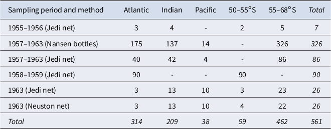

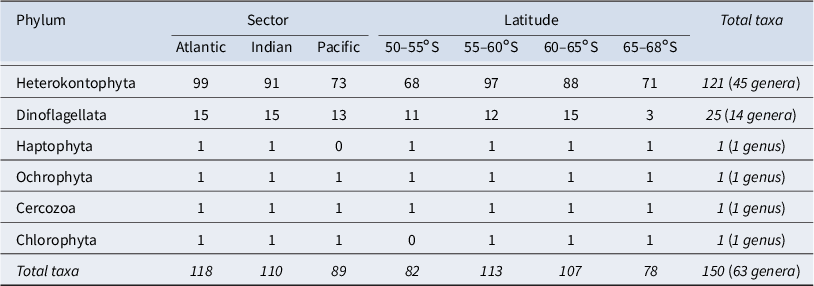
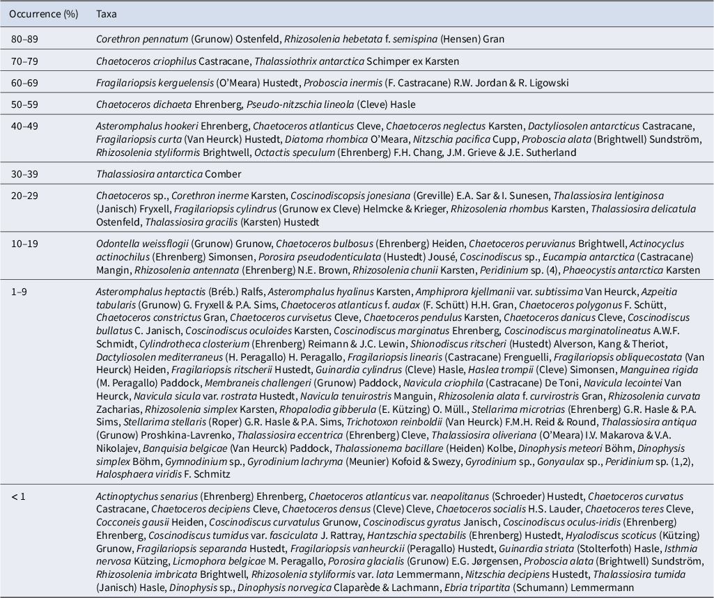
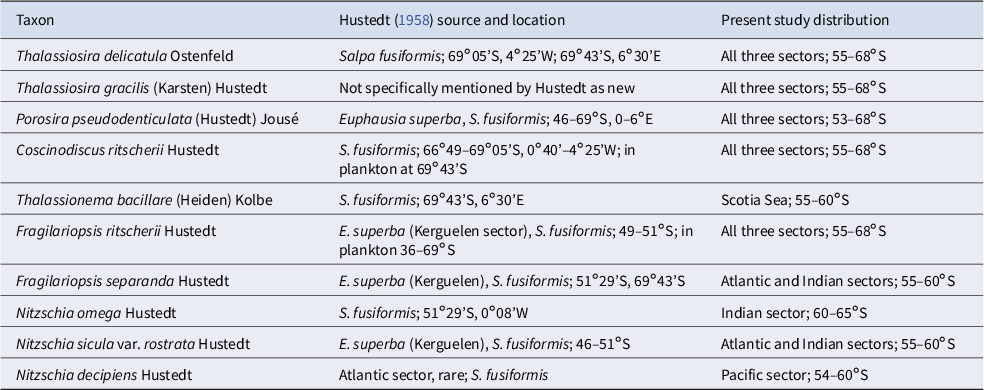
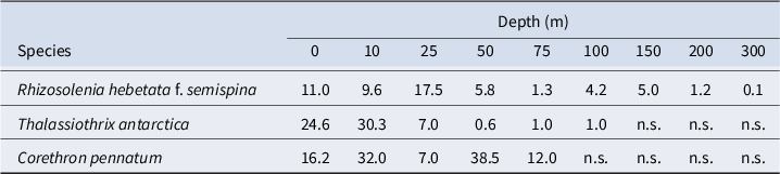

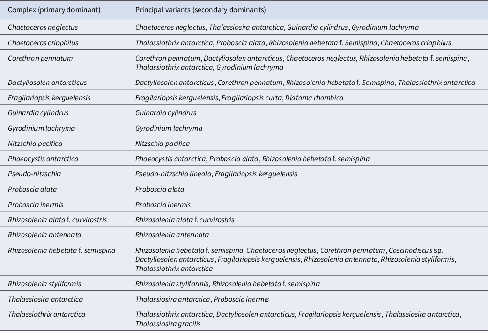
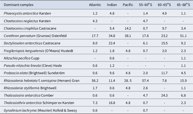
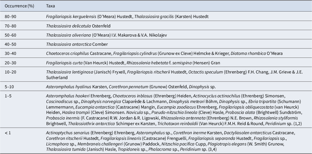
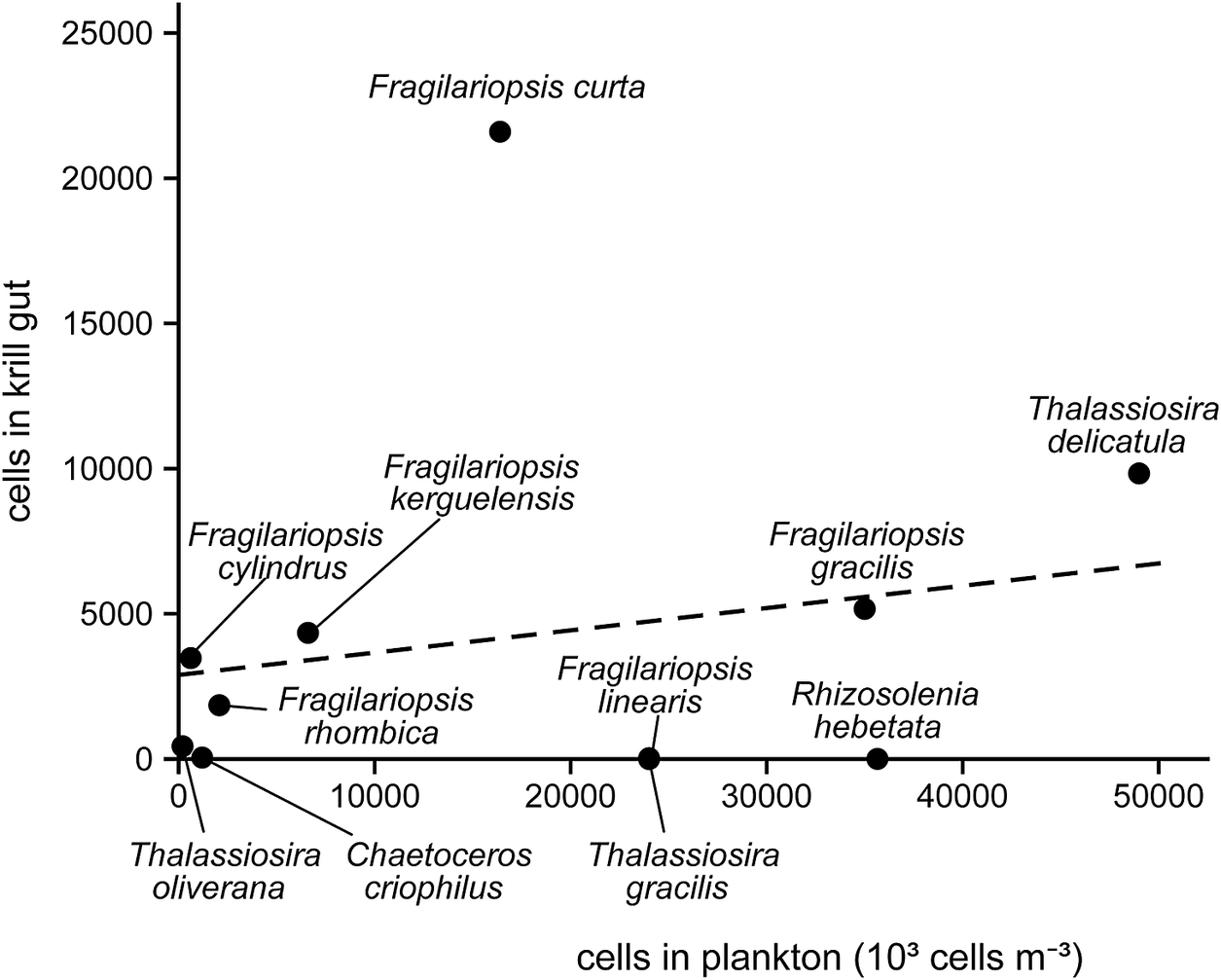


 Open access

