

1 Introduction
Significant effort has been dedicated to the study of turbulent wakes in stratified fluids in recent decades. Classically stratified wake research has focused on naval applications (Pao, Lai & Schemm Reference Pao, Lai and Schemm1982) or large-scale geophysical flows in both the atmospheric and oceanographic settings (Gibson, Nabatov & Ozmidov Reference Gibson, Nabatov and Ozmidov1993; Rotunno, Grubisic & Smolarkiewicz Reference Rotunno, Grubisic and Smolarkiewicz1999; Pawlak et al. Reference Pawlak, MacCready, Edwards and McCabe2003; Perfect, Kumar & Riley Reference Perfect, Kumar and Riley2018). More recently, interest in stratified wakes has resurged due to worldwide interested in wind energy production (Abkar & Porte-Agel Reference Abkar and Porte-Agel2015; Allaerts & Meyers Reference Allaerts and Meyers2018), due to the dynamics of wind-turbine wakes in the nocturnal atmospheric boundary layer. Common to all of these settings is the large initial Reynolds number,  $Re$, based on the diameter of the generating body (or topographic feature), which decreases downstream from the wake. Additionally, a range of internal Froude number,
 $Fr$, values is possible due to changes in the strength of the background stratification. For example, in the context of ocean engineering and marine mammal biology, typically
 $Re\in [10^{6},10^{8}]$ and
 $Fr\in [4,800]$ (Pao et al. Reference Pao, Lai and Schemm1982; Spedding Reference Spedding2014).
It is precisely the resulting combination of highly turbulent flow and stable stratification which leads to the presence of disparate length scales and the persistence of complex, nonlinearly coupled motions at different scales. Such motions include quasi-horizontal ‘pancake’-like vortices, with finer-scale turbulence embedded therein at higher  $Re$, and internal wave radiation by the wake itself. The investigation of such complex phenomena and the establishment of sufficient understanding of the underlying physics is challenging from a theoretical, experimental and computational standpoint. The paper at hand focuses on the energetics and directional properties of internal wave radiation by a stratified wake, in the context of the commonly examined canonical flow of a towed-sphere wake (Spedding Reference Spedding2014). To further put the paper’s primary objective into context, a review of the essential dynamics of the stratified turbulent wake core is first offered. For the interested reader, a thorough overview of both fundamental physics and relevant applications is provided in the review articles of Lin & Pao (Reference Lin and Pao1979) and Spedding (Reference Spedding2014).
1.1 Stratified turbulent wake dynamics
A delineation of the life cycle of a stratified turbulent towed-sphere wake into three regimes is given by Spedding (Reference Spedding1997) for laboratory wakes in which  $5\times 10^{3}\leqslant Re\leqslant 1.2\times 10^{4}$ and
 $4\leqslant Fr\leqslant 240$. For a laboratory-fixed observer, the near-wake or three-dimensional regime occurs for non-dimensional times
 $Nt\leqslant 2$ after the passage of the sphere. During this time, the maximum streamwise-averaged velocity, and the wake width and height, appear to evolve downstream from the body with the same power laws observed for unstratified wakes (Spedding, Browand & Fincham Reference Spedding, Browand and Fincham1996), as derived from self-similarity analysis (Tennekes & Lumley Reference Tennekes and Lumley1972). After
 $Nt\approx 2$, the non-equilibrium (NEQ) regime begins during which the wake is strongly influenced by stratification. While the wake width continues to grow at approximately the same rate, vertical wake growth is halted, and the decay rate of the streamwise-averaged velocity is significantly reduced. Flow structures within the wake become increasingly layered during this period and eventually vertical motions are effectively suppressed: the flow becomes essentially two-dimensional, entering the quasi-two-dimensional (Q2D) regime. At this juncture, any remaining motions in the wake core organize into so-called ‘pancake’ vortices and viscosity ultimately dominates.
The time at which transition from the NEQ to Q2D regime occurs is highly dependent on  $Re$. For laboratory wakes at
 $Re\in [5\times 10^{3},10^{4}]$, Spedding (Reference Spedding1997) find the time of transition to the Q2D regime to be
 $Nt\approx 50$. Similar Q2D transition times are reported by the computational study of Redford, Lund & Coleman (Reference Redford, Lund and Coleman2015) at
 $Re\approx 2.6\times 10^{4}$. A prolongation of the NEQ regime up to
 $Nt\approx 100$ at
 $Re=10^{5}$ is observed in the computational work of Diamessis, Spedding & Domaradzki (Reference Diamessis, Spedding and Domaradzki2011), who conjecture that the NEQ regime could continue up to
 $Nt\geqslant 1000$ in field-scale flows. This prolongation of the NEQ regime is associated with the observation, at
 $Re=10^{5}$ and 4 × 10⁵ (Diamessis et al. Reference Diamessis, Spedding and Domaradzki2011; Zhou & Diamessis Reference Zhou and Diamessis2019), of strong, spatio-temporally intermittent overturning events at times late in the NEQ regime, linked to turbulence resulting from secondary Kelvin–Helmholtz-like instabilities driven by buoyancy-induced vertical shear. Such flow phenomenology is observed in other flows (Riley & de Bruyn Kops Reference Riley and de Bruyn Kops2003; Augier, Chomaz & Billant Reference Augier, Chomaz and Billant2012; de Bruyn Kops & Riley Reference de Bruyn Kops and Riley2019) which are subject to strongly stratified conditions yet possess sufficient separation (dynamic range) between the smallest viscously controlled scale of the turbulent flow and the largest horizontal scale that can overturn against buoyancy. As further elaborated and demonstrated in Zhou & Diamessis (Reference Zhou and Diamessis2019), such flow structure and dynamics are associated with buoyancy having assumed full control over the horizontal integral scale of the flow, as represented by the local (in time) horizontal Froude number,
 $Fr_{h}$, taking on values much smaller than unity. Nevertheless, the corresponding vertical, integral-scale-based, Froude number
 $Fr_{v}$ assumes values close to unity and decays much slower than its horizontal counterpart, enabling the progressively patchier turbulence to overturn. Hereafter, we elect to regard this flow regime, internal to the NEQ regime of Spedding at sufficiently high body-based
 $Re$, as the ‘strongly stratified’ regime. Note that indications of a prolonged NEQ regime have also been reported in the computational studies of Brucker & Sarkar (Reference Brucker and Sarkar2010) and Dommermuth et al. (Reference Dommermuth, Rottman, Innis and Novikov2002) at
 $Re=5\times 10^{4}$ and 105, respectively, although with no observations of turbulent fine structure in the intermediate-to-late wake.
1.2 Internal wave generation by stratified turbulent wakes
An idealized model for a stratified turbulent wake was constructed by Voisin (Reference Voisin1995) where the wake was assumed to consist of a superposition of collapsing of vortex loops or turbulent bursts, which served as simplified representations of the vortex structures inside the wake core. The idealized wake model predicts that the most energetic waves generated by the wake at intermediate to late times propagate at an angle of approximately 55° to the vertical; however, the author notes that this result is highly dependent on the formulation of the wave source, in the form of the above canonical vortex structure representations, used in the model. Additionally it is predicted that the wavelength of gravity waves radiated from the wake will decrease linearly in time.
Bonneton, Chomaz & Hopfinger (Reference Bonneton, Chomaz and Hopfinger1993) towed a sphere through a linearly stratified water tank, generating turbulent wakes in the parameter regime  $Fr\in [1.5,12.7]$,
 $Re\in [380,3\times 10^{4}]$. Both near-body lee waves and ‘random waves’, emitted downstream from the turbulent wake, were observed. Linear theory appears to accurately capture properties of the lee waves. Additionally, it was demonstrated that the properties of the ‘random waves’ were correlated with the coherent structures within the wake.
Spedding et al. (Reference Spedding, Browand, Bell and Chen2000) conducted laboratory experiments towing a sphere through a linearly stratified water tank. The wavelength of internal waves generated by the sphere wake were found to follow a  $Fr^{1/3}$ scaling, which is the same as the one for the wake width. At early times, the radiated waves contained a broad range of frequencies, and hence propagation angles, while, at later times, wave frequencies were found to be associated with the tilting of pancake vortices (see also Plougonven & Zeitlin Reference Plougonven and Zeitlin2002).
Brucker & Sarkar (Reference Brucker and Sarkar2010) compared the wakes generated by towed and self-propelled bodies travelling in both unstratified and linearly stratified domains via numerical experiments at  $Re=5\times 10^{4}$ and
 $Fr=8$. During the early NEQ regime, the energy lost to internal wave radiation was found to dominate over viscous dissipation as a sink for kinetic energy in both the towed and self-propelled cases. The internal wave power continues to decrease throughout the later portion of the NEQ until viscous dissipation again becomes the dominant sink for kinetic energy in the Q2D regime.
Building on the configuration of Diamessis et al. (Reference Diamessis, Spedding and Domaradzki2011), Abdilghanie & Diamessis (Reference Abdilghanie and Diamessis2013) investigated the near-field wave radiation of the wake of a towed sphere at  $Re=5\times 10^{3}$ and
 $Re=10^{5}$ for
 $Fr=4,16,64$ using implicit large-eddy simulations. At the higher
 $Re$, internal wave radiation was found to persist late into the NEQ regime (
 $Nt\approx 100$). The near-field wavelengths and frequencies of the most energetic waves radiated through a fixed horizontal plane above the wake were estimated using one- and two-dimensional wavelet techniques (Dallard & Spedding Reference Dallard and Spedding1993). For higher
 $Re$ and lower
 $Fr$ the wavelength was observed to be smaller, with the initial wavelength determined by the wake height at the beginning of the NEQ regime. For
 $Re=10^{5}$, using the estimated wave frequencies, propagation angles for the most energetic internal waves were inferred to be in the band
 $\unicode[STIX]{x1D703}=45^{\circ }\pm 5^{\circ }$ to the horizontal at earlier times. A general trend towards increasingly horizontal propagation was found as the NEQ regime advances in time. Calculation of the momentum extracted from the wake by wave radiation revealed a significant increase in magnitude at higher
 $Re$, while decreasing with
 $Fr$.
Subsequently, Zhou & Diamessis (Reference Zhou and Diamessis2016) studied the far-field wake-radiated internal wave field, using the same set-up as Abdilghanie & Diamessis (Reference Abdilghanie and Diamessis2013), in albeit deeper and broader domains equipped with a free-slip top surface off which the emitted waves were able to reflect. It was found that the most energetic internal waves, as observed at the model sea surface, were emitted during the very early NEQ regime when the wake is still adjusting to buoyancy. Additionally, the wavelength of the most energetic waves reaching the surface was found to correlate with the vertical Taylor scale (Riley & Lindborg Reference Riley, Lindborg, Davidson, Kaneda and Sreenivasan2012) of the stratified wake turbulence.
Brandt & Rottier (Reference Brandt and Rottier2015) performed laboratory experiments towing a sphere through a linearly stratified water tank, focusing specifically on the internal wave field generated in the low  $Fr$ regime, i.e.
 $Fr\leqslant 4$. Propagation angles of the most energetic internal waves were estimated using phase lines taken from isopycnal contours and were found to be in the range
 $55^{\circ }\leqslant \unicode[STIX]{x1D703}\leqslant 65^{\circ }$. Both body and wake generated internal waves contribute to the overall dynamics. The amplitude of internal wave radiation is found to be largest around
 $Fr=1$, with up to 70 % of the initial energy converted into wave radiation.
Redford et al. (Reference Redford, Lund and Coleman2015) studied a stratified turbulent wake in a linearly stratified fluid using high-resolution direct numerical simulation (DNS) for  $Re=2.6\times 10^{4}$ and
 $Fr=130$. At this relatively high
 $Fr$, the authors concluded that internal wave radiation makes a negligible contribution to the overall energy budget. Calculations of the energy budget were performed in a control volume which spans over the entire computational domain without differentiating between the regions inside and outside the wake region. As such, interpretation of the importance of internal wave radiation to the overall energy budget from their results is difficult due to lumping together the contributions of waves and turbulence to the fluctuating component of the velocity field being in the control volume of choice.
Watanabe et al. (Reference Watanabe, Riley, de Bruyn Kops, Diamessis and Zhou2016) used a statistical analysis conditioned on the enstrophy and potential enstrophy to investigate the properties of a towed-sphere wake in a linearly stratified fluid at  $Re=10^{5}$ and 4 × 10⁵, with a particular focus on the turbulent/non-turbulent interface of the wake cross-section. A high-resolution DNS was initialized with select snapshots of from an implicit large-eddy simulation model (Zhou & Diamessis Reference Zhou and Diamessis2016) and was run for short time intervals in the early NEQ regime. At the particular times considered, the rate of energy loss due to internal wave radiation was found to be comparable to that of viscous dissipation of kinetic energy inside the wake core.
1.3 Objectives and overview
Despite the extensive research conducted on internal wave radiation emitted from stratified turbulent wakes, a number of open questions remain: What fraction of wake kinetic energy is lost to internal wave radiation at each instant in time over the entire wake life cycle? At which points in the wake life cycle are the most energetic internal waves emitted and from which locations on the wake periphery? What is the direction of propagation of wave radiation in the near field? In the context of these questions, how do waves emitted early in the NEQ regime compare to those generated by turbulence operating in the strongly stratified regime at later times at higher  $Re$?
Motivated by the above questions and relying on pointwise estimates of the energy flux vector, the present study first aims to quantify the total amount of wake energy lost to internal wave radiation as a function of Reynolds and Froude numbers – and, corollary to this effort – whether a universally applicable parametric dependence exists allowing for comparison with field-scale wakes. This work seeks to contrast the contribution to the internal wave field radiated by turbulence subject to the onset of buoyancy control – upon the establishment of the NEQ regime – to that of the highly layered turbulence in the strongly stratified regime, which subsequently emerges in the wake core at higher  $Re$. In addition, the relative importance of internal wave radiation as a sink for wake kinetic energy will be investigated. Finally, the directionality of the internal wave radiation will be explored and compared to the results obtained from linear theory. In this same context, the preferred locations of wave radiation along the wake edge are also identified.
The remaining text is structured as follows. In § 2 the procedure used to conduct numerical experiments is given, including the model equations, boundary conditions, algorithm and resolutions utilized. The kinetic energy budget is then discussed with particular emphasis on the difference in the physical interpretation of relevant terms between the turbulence and internal wave literature. The procedure for calculation of the wave power radiated from the wake is also presented. Section 4 contains results from numerical experiments which are presented in a succinct manner, reserving discussion of these results for § 5. Connections to the broader literature will be made in this discussion as well. Section 6 offers concluding remarks.
2 Methodology
2.1 Temporal evolution of intermediate-to-far wake
At sufficiently high Reynolds number, wake motions can persist in excess of 103 to 105 sphere diameters downstream (Spedding Reference Spedding2014). In close proximity to the sphere, fine-scale motions are present such as the turbulent boundary layer on the sphere’s surface and the vortices shed from therein. Consequently, conducting a numerical simulation which spans the entire life cycle of the turbulent wake, i.e. its full downstream evolution, requires prohibitively significant computing resources due to the high resolution necessary in the near wake and large computational domain needed to capture the spatial wake evolution far downstream. Although a simulation of this magnitude will likely become feasible sometime in coming decades, an alternative approach is necessary at the present.
As discussed in greater detail in § 2.3 of Zhou & Diamessis (Reference Zhou and Diamessis2016), under the assumption that turbulence is locally homogeneous in the direction parallel to the wake centreline, a less computationally costly approach consists of simulating a segment of the wake downstream from the sphere by assuming temporal wake evolution within a finite horizontally periodic domain in a laboratory-fixed reference frame (Orszag & Pao Reference Orszag and Pao1975). An approximation of the mean and turbulent velocity fields a short distance downstream from the sphere is then made to construct the initial conditions for such a simulation (Diamessis et al. Reference Diamessis, Spedding and Domaradzki2011). Previous studies of temporally evolving wakes have successfully employed this approach (Gourlay et al. Reference Gourlay, Arendt, Fritts and Werne2001; Dommermuth et al. Reference Dommermuth, Rottman, Innis and Novikov2002; Diamessis, Domaradzki & Hesthaven Reference Diamessis, Domaradzki and Hesthaven2005; Redford et al. Reference Redford, Lund and Coleman2015).
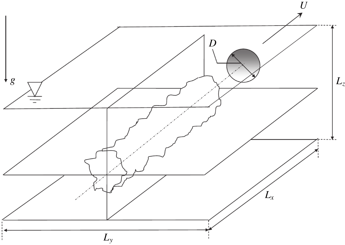
Computational domain for the simulation of temporally evolving, stratified towed-sphere wake datasets analysed in this study. The centreline of the wake is at  $(y,z)=(0,0)$. The towed sphere is not accounted for explicitly in the simulations and is, instead, introduced through a complex initialization procedure (Diamessis et al. Reference Diamessis, Spedding and Domaradzki2011). The sphere is assumed to be towed along the
 $x$-axis which is the only statistically homogeneous direction in these simulations.

2.2 Model equations
In the present study a three-dimensional Cartesian coordinate system is utilized with the  $x$-axis parallel to the wake centreline and the positive
 $z$-axis antiparallel to gravitational force, as seen in figure 1. The incompressible Navier–Stokes equations under the Boussinesq approximation (Spiegel & Veronis Reference Spiegel and Veronis1960) are used as the governing equations. As such, the fluid density is decomposed into two components,
 $$\begin{eqnarray}\unicode[STIX]{x1D70C}(\boldsymbol{x},t)=\bar{\unicode[STIX]{x1D70C}}(z)+\unicode[STIX]{x1D70C}^{\prime }(\boldsymbol{x},t),\end{eqnarray}$$
where  $\bar{\unicode[STIX]{x1D70C}}$ is the vertically varying background density and
 $\unicode[STIX]{x1D70C}^{\prime }$ is the deviation from this background density due turbulence or internal wave contributions to the fluid motion. Using the value of background density at the bottom of the domain,
 $\unicode[STIX]{x1D70C}_{0}=\bar{\unicode[STIX]{x1D70C}}(0)$, as a reference value the Boussinesq approximation requires that the background density varies in the vertical under the constraint that
 $$\begin{eqnarray}\frac{\unicode[STIX]{x1D6FF}\unicode[STIX]{x1D70C}(z)}{\unicode[STIX]{x1D70C}_{0}}=\frac{\bar{\unicode[STIX]{x1D70C}}(z)-\unicode[STIX]{x1D70C}_{0}}{\unicode[STIX]{x1D70C}_{0}}\ll 1.\end{eqnarray}$$
Additionally, perturbations to the background density produced by either turbulence or internal waves are such that
 $$\begin{eqnarray}\unicode[STIX]{x1D70C}^{\prime }\ll \bar{\unicode[STIX]{x1D70C}}(z)-\unicode[STIX]{x1D70C}_{0}.\end{eqnarray}$$
If  $\boldsymbol{u}(\boldsymbol{x},t)$ is the fluid velocity, the governing equations can be written in the form
 $$\begin{eqnarray}\displaystyle & \displaystyle {\displaystyle \frac{\unicode[STIX]{x2202}\boldsymbol{u}}{\unicode[STIX]{x2202}t}}+\left(\boldsymbol{u}\boldsymbol{\cdot }\unicode[STIX]{x1D735}\right)\boldsymbol{u}=-{\displaystyle \frac{1}{\unicode[STIX]{x1D70C}_{0}}}\unicode[STIX]{x1D735}p^{\prime }-{\displaystyle \frac{\unicode[STIX]{x1D70C}^{\prime }\,g}{\unicode[STIX]{x1D70C}_{0}}}\boldsymbol{e}_{\boldsymbol{z}}+\unicode[STIX]{x1D708}\unicode[STIX]{x1D6FB}^{2}\boldsymbol{u}, & \displaystyle\end{eqnarray}$$
 $$\begin{eqnarray}\displaystyle & \displaystyle {\displaystyle \frac{\unicode[STIX]{x2202}\unicode[STIX]{x1D70C}^{\prime }}{\unicode[STIX]{x2202}t}}+\left(\boldsymbol{u}\boldsymbol{\cdot }\unicode[STIX]{x1D735}\right)\unicode[STIX]{x1D70C}^{\prime }=-w{\displaystyle \frac{\unicode[STIX]{x2202}\bar{\unicode[STIX]{x1D70C}}}{\unicode[STIX]{x2202}z}}+\unicode[STIX]{x1D705}\unicode[STIX]{x1D6FB}^{2}\unicode[STIX]{x1D70C}^{\prime }, & \displaystyle\end{eqnarray}$$
 $$\begin{eqnarray}\displaystyle & \displaystyle \unicode[STIX]{x1D735}\boldsymbol{\cdot }\boldsymbol{u}=0, & \displaystyle\end{eqnarray}$$
 $p^{\prime }$ represents the pressure perturbation to the background hydrostatic pressure.
The background density profile,  $\bar{\unicode[STIX]{x1D70C}}(z)$, for the numerical experiments described in § 2.3 is chosen to be linear linear; consequently, the Brunt–Väisälä or buoyancy frequency, given by
 $$\begin{eqnarray}N^{2}(z)=-\frac{g}{\unicode[STIX]{x1D70C}_{0}}\frac{\text{d}\bar{\unicode[STIX]{x1D70C}}}{\text{d}z},\end{eqnarray}$$
is constant (Olbers, Willebrand & Eden Reference Olbers, Willebrand and Eden2012) and will hereafter be denoted as  $N$. Physically, this approximates realistic oceanic density profiles over a relatively short vertical extent – in the thermocline or deep ocean, for example.
2.3 Large-eddy simulation datasets
The datasets analysed herein originate from eight implicit large-eddy simulations (LES) of stratified turbulent wakes, documented in full detail in Zhou (Reference Zhou2015) and Zhou & Diamessis (Reference Zhou and Diamessis2019): only a brief account will be provided subsequently.
The computational domain of the LES has length, width and height denoted  $L_{x}$,
 $L_{y}$ and
 $L_{z}$, respectively. The origin of the Cartesian coordinate system is chosen to be on the centreline of the towed sphere, as shown in figure 1. The values of
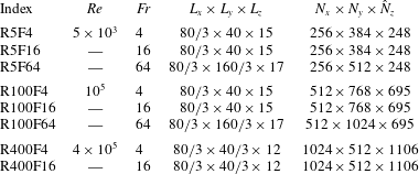
 $Re$ and
 $Fr$ used for each case are given in table 1. The simulations are run from an initial time corresponding to a downstream distance of
 $x/D=2$ from the towed sphere to the beginning of the Q2D regime or even later therein. The corresponding final times are
 $Nt_{f}\approx 120$, 240 and 1000 for
 $Re=5\times 10^{3}$, 105 and 4 × 10⁵ respectively. The number of points used in the computational grid has been chosen to ensure that a significant portion of the inertial subrange is well resolved whenever present during the wake evolution, particularly at the two higher
 $Re$ values. Comparison with DNS simulations, initialized with LES data and run over shorter time windows such that the full range of scales of turbulence inside the wake score is populated, shows that all numerical experiments considered here are resolved to at least
 $20\unicode[STIX]{x1D702}$, where
 $\unicode[STIX]{x1D702}$ is the DNS-computed Kolmogorov scale (Zhou Reference Zhou2015; Watanabe et al. Reference Watanabe, Riley, de Bruyn Kops, Diamessis and Zhou2016).
Summary of numerical simulations at various wake Reynolds and Froude numbers.  $L_{x}$,
 $L_{y}$ and
 $L_{z}$ are the domain dimensions – in units of body diameters,
 $D$ – and
 $N_{x}\times N_{y}\times \hat{N}_{z}$ is the number of grid points. Here
 $\hat{N}_{z}$ is the number of grid points allocated to the interval
 $z/D\in [-6,6]$, which corresponds to the full vertical extent of the computational domain for the R400 simulations. The Prandtl number,
 $Pr=\unicode[STIX]{x1D708}/\unicode[STIX]{x1D705}$, is set to unity.

2.3.1 Numerical method
The governing (2.4) are solved using the algorithm described in Diamessis et al. (Reference Diamessis, Domaradzki and Hesthaven2005). A pseudospectral Fourier discretization is used in the horizontal, while a Legendre-polynomial-based spectral multi-domain penalty method is used in the vertical. Such a discretization optimally allows for a high degree of accuracy to be obtained while using fewer grid points than would be required by a conventional low-order method. Additionally, the use of a multi-domain method in the vertical allows for the concentration of grid points where resolution is needed in the centre of the wake. In terms of temporal discretization, the velocity, density and pressure are advanced using a stiffly stable, third-order, implicit–explicit (IMEX) scheme (Karniadakis, Israeli & Orszag Reference Karniadakis, Israeli and Orszag1991).
2.3.2 Filtering
Simulations presented herein, while not reaching the Kolmogorov scale,  $\unicode[STIX]{x1D702}$, resolve flows down to within
 $~20\unicode[STIX]{x1D702}$ in most cases. As such, it is assumed that a sub-grid-scale model is unnecessary. Numerical stability, however, is ensured through the application of an exponential filter in spectral space – in both horizontal and vertical directions. Details of the specific filter functions used in this study may be found in Zhou (Reference Zhou2015). Such a low-pass filter removes energy from the smallest resolved scales, while not directly impacting moderate and large-scale motions (Diamessis et al. Reference Diamessis, Spedding and Domaradzki2011).
2.3.3 Initial and boundary conditions
The study at hand follows Diamessis et al. (Reference Diamessis, Spedding and Domaradzki2011) and uses initial conditions from both mean and fluctuating velocity profiles derived from the assumption of a self-similar mean velocity profile near the sphere (Meunier, Diamessis & Spedding Reference Meunier, Diamessis and Spedding2006). The interested reader is referred to Diamessis et al. (Reference Diamessis, Spedding and Domaradzki2011) for a more detailed discussion which also elaborates on how correlation between mean and fluctuating velocity fields is established by virtue of a relaxation procedure and how the background stratification is progressively ‘turned on’ to minimize spurious restratification transients. A review of the salient points of this initialization may be found in Zhou & Diamessis (Reference Zhou and Diamessis2016).
Boundary conditions on all variables are inherently periodic in both horizontal directions. Care is taken that the domain is always sufficiently long to accommodate an adequate number of streamwise turbulence integral scales. Regular regridding (Diamessis et al. Reference Diamessis, Spedding and Domaradzki2011) in the spanwise direction is performed to avoid spurious interactions with the wake’s its periodic image. Sponge layers (see Abdilghanie Reference Abdilghanie2010, for details on their implementation in the context of the governing equations) are placed on both lateral boundaries of the computational domain to prevent spurious re-entry of the wake-radiated internal waves.
In the vertical, free-slip boundary conditions were used on the top of the computational domain, while no-slip conditions were imposed at the bottom. Density perturbations were taken to vanish on the top and bottom boundaries. However, to prevent internal wave reflection, the bottom boundary of the computational domain for all  $Re$ and
 $Fr$ simulations is also equipped with sponge layers. Sponge layers are only inserted at the top boundary of the
 $Re=4\times 10^{5}$ datasets due to the reduced lateral and vertical dimensions of the associated computational domains. Since the
 $Re=5\times 10^{3}$ and 105 simulations were designed with the objective of examining the surface manifestation of internal waves (Zhou & Diamessis Reference Zhou and Diamessis2016), their upper boundary does not have a sponge layer; nonetheless, visualizations of the horizontal divergence of the velocity field indicate that the top-surface-reflected internal waves do not interact significantly with the wake near field over the course of these simulations.
The instantaneous pressure perturbation  $p^{\prime }$ field for any given wake flow snapshot is computed by solving a Poisson equation which is obtained by taking the divergence of (2.4a) and applying the incompressibility condition (2.4c). In the vertical direction, inhomogeneous Neumann boundary conditions are used for
 $p^{\prime }$, which result from the vertical momentum equation applied to an impermeable boundary with zero density perturbations.
3 Internal wave energetics
3.1 Kinetic energy budget
One of the primary goals of the current study is to determine the contribution of internal wave radiation to the dynamics of a stratified turbulent wake, in particular, its relative importance as a sink for kinetic energy. The kinetic energy density
 $$\begin{eqnarray}E_{k}={\textstyle \frac{1}{2}}\unicode[STIX]{x1D70C}_{0}\Vert \boldsymbol{u}\Vert ^{2}\end{eqnarray}$$
satisfies the conservation law
 $$\begin{eqnarray}\frac{\unicode[STIX]{x2202}E_{k}}{\unicode[STIX]{x2202}t}+\unicode[STIX]{x1D735}\boldsymbol{\cdot }(\boldsymbol{u}E_{k})=-\unicode[STIX]{x1D735}\boldsymbol{\cdot }(p^{\prime }\boldsymbol{u})-\unicode[STIX]{x1D70C}^{\prime }gw+2\unicode[STIX]{x1D708}\unicode[STIX]{x1D735}\boldsymbol{\cdot }(\boldsymbol{u}\boldsymbol{\cdot }\unicode[STIX]{x1D64E})-2\unicode[STIX]{x1D708}\unicode[STIX]{x1D64E}\boldsymbol{ : }\unicode[STIX]{x1D64E},\end{eqnarray}$$
where
 $$\begin{eqnarray}\unicode[STIX]{x1D64E}=\unicode[STIX]{x1D61A}_{ij}\equiv \frac{1}{2}\left(\frac{\unicode[STIX]{x2202}u_{i}}{\unicode[STIX]{x2202}x_{j}}+\frac{\unicode[STIX]{x2202}u_{j}}{\unicode[STIX]{x2202}x_{i}}\right)\end{eqnarray}$$
is the strain-rate tensor. Integrating (3.2) over a control volume,  ${\mathcal{V}}(t)$, with a bounding surface,
 $\unicode[STIX]{x2202}{\mathcal{V}}(t)$, and rearranging terms gives the energy budget for the total kinetic energy,
 ${\mathcal{E}}_{k}$
 $$\begin{eqnarray}\frac{\text{d}{\mathcal{E}}_{k}}{\text{d}t}=-\oint _{\unicode[STIX]{x2202}{\mathcal{V}}(t)}\{(\boldsymbol{u}-\boldsymbol{u}_{s})E_{k}+p^{\prime }\boldsymbol{u}-2\unicode[STIX]{x1D708}\,\boldsymbol{u}\boldsymbol{\cdot }\unicode[STIX]{x1D64E}\}\boldsymbol{\cdot }\hat{\boldsymbol{n}}\,\text{d}S-\int _{{\mathcal{V}}(t)}(\unicode[STIX]{x1D70C}^{\prime }gw+2\unicode[STIX]{x1D708}\unicode[STIX]{x1D64E}\boldsymbol{ : }\unicode[STIX]{x1D64E})\,\text{d}V.\end{eqnarray}$$
If  $\unicode[STIX]{x2202}{\mathcal{V}}(t)$, is a material surface then
 $\boldsymbol{u}|_{\unicode[STIX]{x2202}{\mathcal{V}}}=\boldsymbol{u}_{s}$, and the advective terms in (3.4) vanish. The terms in the surface integral represent the rate of extra-volumetric transport of kinetic energy due to advection, work done by pressure and work done against viscous stress, respectively. The terms in the volume integral represent the intra-volumetric rate of conversion of kinetic energy to potential and internal energy due to work done against buoyancy and viscous dissipation, respectively. For a closed control volume, as is often considered in space-filling turbulence studies, the surface integral terms are typically taken to vanish. In the current context however, open control volumes will be considered and the surface integral terms will be an important sink for kinetic energy.
Presently no appeal will be made to the Reynolds decomposition; instead, the wake region will be defined to include both the mean and turbulent components of the wake. Additionally, the control surface used in the kinetic energy budget analysis (3.2) is constructed to remain outside the wake region – allowing the pressure-work term to be interpreted solely as the power flux due to internal wave radiation. Conceding the possibility of internal waves being generated and remaining within the wake region, no distinction will be made between the energy of such trapped waves and that of the wake. Collectively these choices facilitate a concise analysis.
Finally, the question arises as to whether work done by or against the hydrostatic pressure gradient may be neglected in the kinetic energy budget (3.4), where currently only the contribution of the corresponding perturbation pressure appears. In this study, it is emphasized that the calculation of radiated internal wave power and the associated directional preferences of the wave field is restricted to the region immediately exterior of the turbulent wake – particularly as demarcated by the wake-following elliptic cylinder discussed in § 3.2. By the criterion used to construct the elliptic cylinder, the mean velocity on this control surface must vanish; further, the buoyancy frequency in the region exterior to the cylinder is constant. Consequently, linear theory indicates that all power in the radiated wave field is driven by the perturbation pressure with no contribution from the hydrostatic component. To avoid diffusing the scope of the paper at hand, the interested reader is referred to Lamb (Reference Lamb2007) for a more in-depth discussion with additional theoretical background found in Bühler (Reference Bühler2014).
3.2 Flux calculation
To precisely calculate the total energy lost by the wake to internal wave radiation, a control volume is needed which allows a sharp separation of the wake from the surrounding fluid. Such a distinction requires an accurate definition of the turbulent/non-turbulent interface of the wake. Many studies have devoted effort in this pursuit and, in the case of a stratified wake, it has been found by Watanabe et al. (Reference Watanabe, Riley, de Bruyn Kops, Diamessis and Zhou2016) that combined thresholding of both the enstrophy and potential enstrophy fields provide the necessary criterion. Ultimately, the goal of this study is the quantification of energy radiated from the wake by internal waves: utilizing a surface which bounds the wake tightly, but not exactly, will provide a sufficiently accurate and reliable answer. An elliptic cylinder approximates the shape of the wake well and the flux integrals on this surface can then be easily computed. Such a brute-force approach was chosen for its simplicity; however, it must be reiterated that more refined techniques are available. An example of a more sophisticated technique, which is likely to enable the computation of the exact energy flux at the precisely identified turbulent/non-turbulent interface (Watanabe et al. Reference Watanabe, Riley, de Bruyn Kops, Diamessis and Zhou2016), is the very recent work of Shete & de Bruyn Kops (Reference Shete and de Bruyn Kops2020). Application of such an approach to the turbulent wake will be the subject of future work.
The wave power radiated through an elliptic cylinder is given by
 $$\begin{eqnarray}{\mathcal{P}}(t)=\oint _{\unicode[STIX]{x1D6E4}}\int _{0}^{L_{x}}p^{\prime }\boldsymbol{u}\boldsymbol{\cdot }\hat{\boldsymbol{n}}\,\text{d}x\,\text{d}s,\end{eqnarray}$$
where  $\hat{\boldsymbol{n}}$ is the unit vector normal to the cylinder, and
 $\unicode[STIX]{x1D6E4}$ is a closed circuit tracing the elliptic cross-section of the cylinder anticlockwise. The height and width of the wake are time dependent, implying that the dimensions of the elliptic cylinder should also vary in time. In the present study an indicator function, defined to be unity in the region where the streamwise-averaged kinetic energy, normalized by its maximum value, is greater than 5 × 10⁻³ and vanishing elsewhere, was used to define the elliptic cross-section. The centroid of the indicator function is used to define the centre of the ellipse, and 1.5 times the square root of the horizontal and vertical variance is used to define the major and minor axes, respectively. Application of this approach was found to provide a tight bound for the wake without requiring the calculation of the enstrophy and potential enstrophy.
At a given instant in time, the pressure–velocity product,  $p^{\prime }\boldsymbol{u}$ is interpolated onto the elliptic cylinder using spectral interpolation, consisting of two-dimensional Fourier interpolation in the horizontal directions and element-based high-order Lagrange interpolation in the vertical. Fourier quadrature is then used to compute the subsequent surface integral. Fastidious readers are referred to appendix A for a more detailed explanation of this procedure.
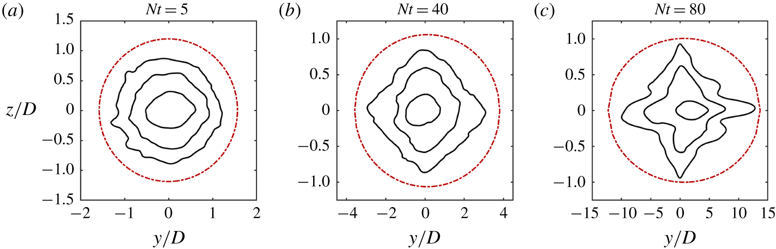
Figure 2 demonstrates the fit of the elliptic cylinder at three times for the  $Re=10^{5}$,
 $Fr=4$ case. The solid (black) contours of the streamwise-mean kinetic energy correspond to values which are 0.5 %, 5 % and 50 % of the maximum value at each time. The dashed (red) contour demonstrates the cross-section of the elliptic cylinder used for the flux calculation. The aspect ratio of each panel has been adjusted to be uniform for comparison purposes, however, the horizontal axis reveals that the wake has a very high aspect ratio at later times. The eccentricity of the elliptic cylinder (see appendix A) at
 $Nt=80$ is approximately 0.99.
Cross-sections of the streamwise-mean kinetic energy for  $Re=10^{5}$,
 $Fr=4$. Solid (black) contours correspond to values of 0.5 %, 5 % and 50 % of the maximum value at each time. The dashed (red) contour shows the fit of the elliptic cylinder used for the wave flux calculation.

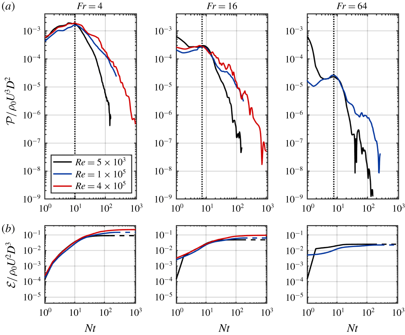
The instantaneous wave power (a) and total wave energy (b) radiated through a wake-following elliptic cylinder, scaled by  $\unicode[STIX]{x1D70C}_{0}U^{3}D^{2}$ and
 $\unicode[STIX]{x1D70C}_{0}U^{2}D^{3}$ respectively.

Repeated tests have shown that all the potential enstrophy in the flow is contained within the limits of the elliptic cylinder. Consequently, only internal waves, and not turbulent motions inside the wake region, contribute to the pressure–velocity product,  $p^{\prime }\boldsymbol{u}$ (Watanabe et al. Reference Watanabe, Riley, de Bruyn Kops, Diamessis and Zhou2016) when computed on the surface of the elliptic cylinder. Moreover, given the relatively compact fit of the elliptic cylinder around the wake core, the contributions to
 $p^{\prime }\boldsymbol{u}$ originate from waves generated relatively recently with respect to the time of observation. Sampling internal wave signatures close to the wake allows a clearer identification and separation of the contributions to internal wave radiation of very early, three-dimensional actively turbulent wake and its subsequent adjustment to buoyancy in the early NEQ regime, and later-time turbulence operating in the strongly stratified regime. Specifically, in contrast to the case of measuring internal wave properties at a remote location sufficiently removed from the wake (Zhou & Diamessis Reference Zhou and Diamessis2016), the time lag between any observation of wave activity on the elliptic cylinder and the process of wave generation by turbulence in the wake interior is minimal to negligible. Finally, the tight bound provided by the elliptic cylinder ensures there is insufficient time for viscosity to attenuate internal waves before they reach the control surface.
4 Results
4.1 Radiated internal wave power
Time series of the instantaneous wave power radiated through the elliptic cylinder – described in § 3.2 – are shown in figure 3(a), with all of the experiments for a single value of  $Fr$ on the same panel. A turning point in the wave power flux occurs at
 $Nt\approx 10$ for all cases, at which time the wave power has approximately the same magnitude for all cases with the same
 $Fr$. After the turning point, the power of the wave radiation decreases for all later times across all cases. The decrease in wave power is more gradual at
 $Re=10^{5}$ and
 $Re=4\times 10^{5}$ for which the late time power is approximately 10 times larger than the
 $Re=5\times 10^{3}$ experiments.
Figure 3(b) shows time series for the corresponding cumulative wave energy radiated through the elliptic cylinder. For all experiments, the radiated wave energy increases, asymptotically approaching a maximum value at late times. The total wave energy decreases approximately half an order of magnitude as the value of  $Fr$ is increased from 4 to 16 to 64. While the total wave energy increases with increasing
 $Re$ for the
 $Fr=4$ and 16 experiments, the total wave energy is approximately the same for both experiments with
 $Fr=64$.
The similarity of all curves suggests that a parametric scaling can be found which will collapse the time series. Per the discussion of § 4.4, the wave power appears to be one of the leading-order terms in the volume-integrated kinetic energy equation (3.4) at  $Nt\approx 10$ – the time of peak radiated wave power. Therefore, a scaling following the rate of change of wake kinetic energy is pursued. Spedding (Reference Spedding1997) and Diamessis et al. (Reference Diamessis, Spedding and Domaradzki2011) find the maximum streamwise-averaged velocity of a stratified turbulent wake scales as
 $Fr^{-2/3}$, while the wake width follows a
 $Fr^{1/3}$ scaling. Consequently, one expects the rate of change of kinetic energy per unit volume within the wake region to scale as
 $U_{0}^{3}/L_{H}$ and, therefore,
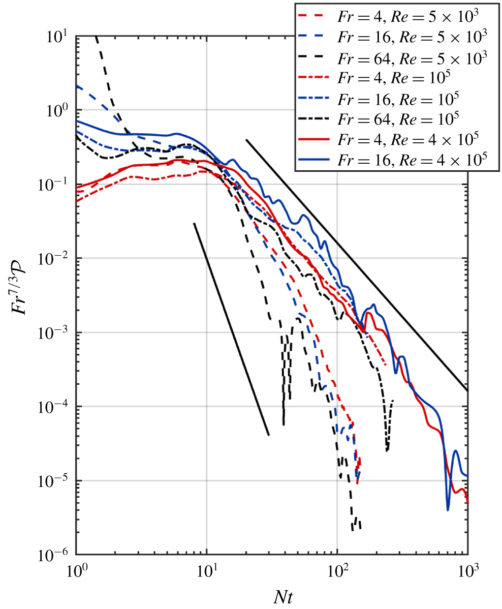
 $Fr^{-7/3}$. Indeed, the time series of the wave power per unit volume do collapse, namely around the time of peak wave power radiation, when the vertical axis is scaled with
 $Fr^{7/3}$ (figure 4). Although a theoretical interpretation remains to be offered in terms of observed power law exponents, the lower
 $Re$ time series have a tail that appears to decay as
 $Nt^{-5}$. In contrast, the corresponding tails for the two higher
 $Re$ datasets are subject to a slower decay of
 $Nt^{-2}$.
Scaled wave power time series from elliptic cylinder analysis. The upper and lower solid lines have a slope of - 2 and - 5 respectively. The wave power is scaled by the volume of the elliptic cylinder.

4.2 Location of most intense wave radiation
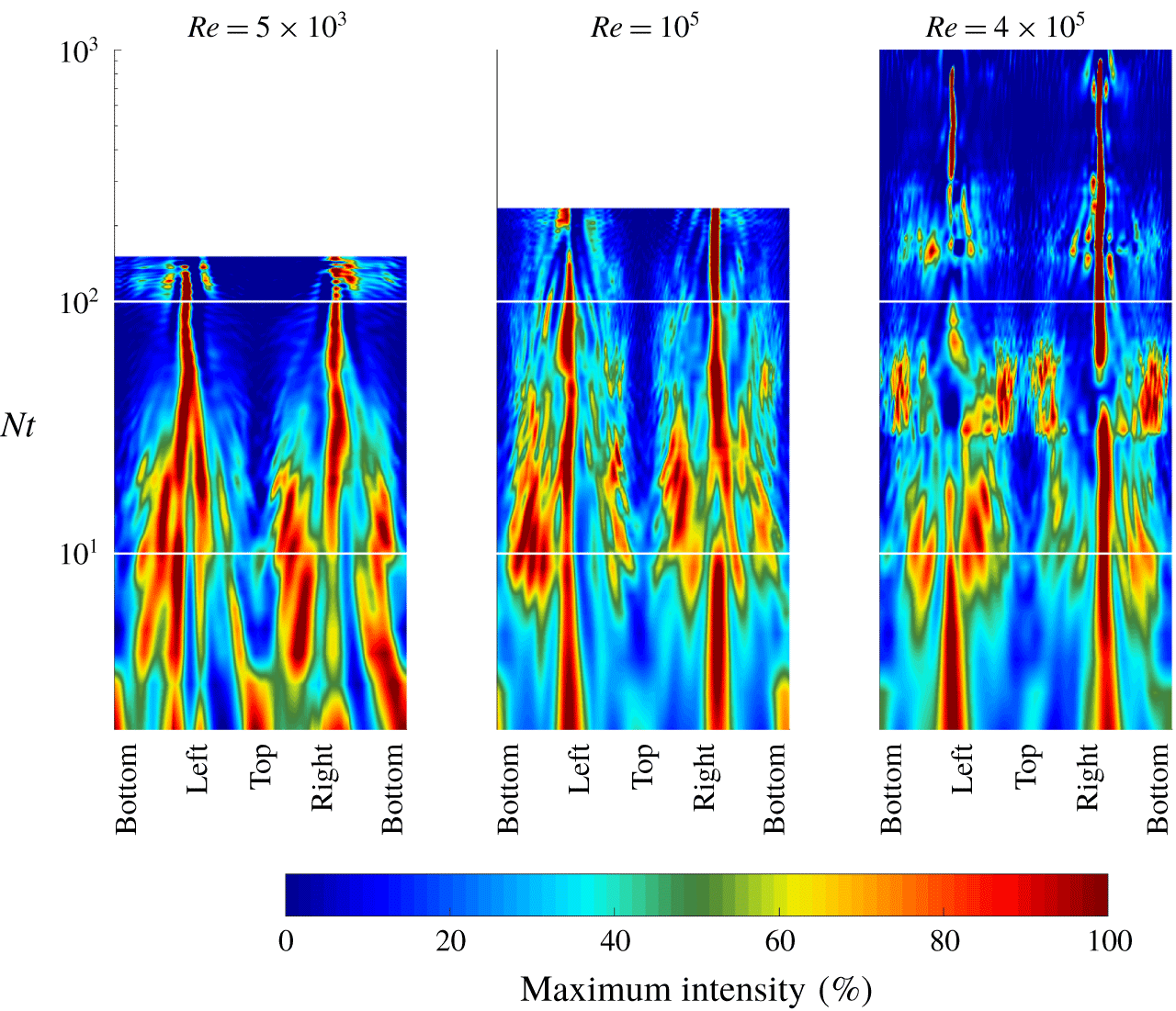
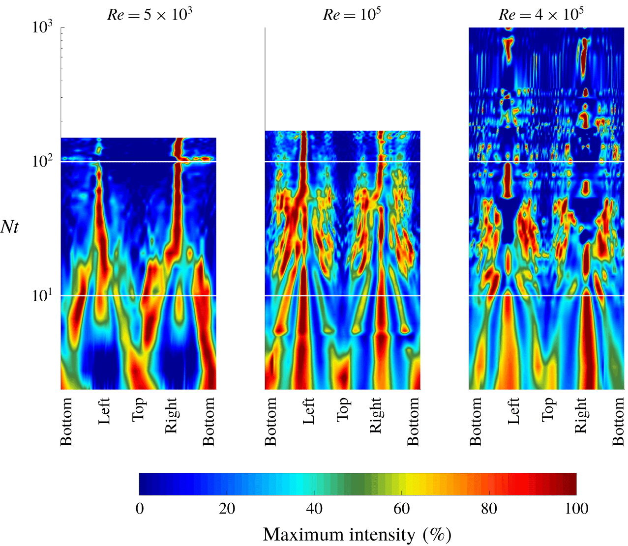
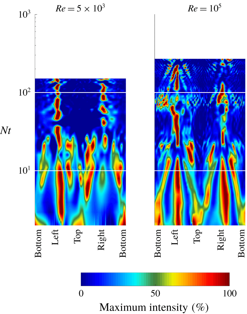
The space–time contours of streamwise-mean wave power flux or intensity,  $I$, normal to the surface of a wake-following elliptic cylinder are shown in figures 5 through 7. Here,
 $I$ is defined as
 $$\begin{eqnarray}I(s,t)=\frac{1}{L_{x}}\int _{0}^{L_{x}}p^{\prime }\boldsymbol{u}\boldsymbol{\cdot }\hat{\boldsymbol{n}}\,\text{d}x.\end{eqnarray}$$
The horizontal axis of each figure corresponds to the tangential coordinate,  $s$, around the cylinder cross-section: the arc length of a circuit traced anticlockwise from the bottom, normalized by the circumference of this ellipse. In addition, at each
 $Nt$ value in the time series, the mean wave intensity has further been normalized as a percentage of the instantaneous maximum value. Due to the fact that wave power diminishes rapidly in time, such a normalization allows for a demonstration of the spatial distribution of the mean wave intensity in a manner conducive to straightforward comparison across different times and
 $Re$ and
 $Fr$.
Space–time contours of internal wave intensity normal to a wake-following elliptic cylinder, scaled at each time as a per cent of the instantaneous maximum, for the  $Fr=4$ simulations. Horizontal axes display the tangential coordinate around the cylinder cross-section. The horizontal white lines mark times
 $Nt=10$ and 100.

Space–time contours of internal wave intensity for the  $Fr=16$ simulations. Labels follow the convention described in the caption of figure 5.

Space–time contours of internal wave intensity for the  $Fr=64$ simulations. Labels follow the convention described in the caption of figure 5.

Figure 5 corresponds to the numerical experiments with  $Fr=4$. At early times,
 $Nt\leqslant 20$, in the
 $Re=5\times 10^{3}$ case, the wave intensity throughout a considerable fraction of the elliptic cylinder is within 50 % of the peak value; although a bias towards the top and bottom of the wake, and its left and right edges, is observed. As time progresses, wave intensity becomes patchily distributed, with a slight preference for locations on the wake periphery which are sufficiently removed from top, bottom, left and right edges. After
 $Nt\approx 20$, there is a clear trend towards the left and right edges of the cylinder. In contrast, the
 $Re=10^{5}$ and 4 × 10⁵ cases shows a clear bias towards the left and right sides of the wake up to
 $Nt\approx 10$. Wave intensity is intermittent at intermediate times,
 $10\leqslant Nt\leqslant 20$, before trending towards the wake sides at late times.
Wave intensity for simulations with  $Fr=16$ is shown in figure 6. For the lowest
 $Re$ case, wave intensity is initially greatest at the top and bottom of the wake, before becoming distributed around the circumference of the wake in the range
 $4\leqslant Nt\leqslant 20$. After this point, wave intensity is strongest at the left and right edges in a manner similar to the
 $Fr=4$ simulation. For the higher
 $Re$ cases, intensity is initially largest at the top, bottom, left and right edges until
 $Nt\approx 20$. As time advances, at
 $Nt\approx 20$ and afterward, the radiation pattern is considerably more patchy or intermittent than for the lower
 $Re$ experiments. At late times, a weak trend towards the sides of the wake is observed for
 $Re=10^{5}$, however the wave intensity is highly intermittent for the
 $Re=4\times 10^{5}$ case.
Lastly, figure 7 corresponds to the  $Fr=64$ experiments. Trends are not as coherent here as for the
 $Fr=4$ and 16 cases, however there is a weak preference for the left and right wake edges from
 $Nt\geqslant 20$.
4.3 Emission angles of the most intense wave radiation
For vertically propagating internal waves in the absence of a mean flow, the wave power-flux vector,  $p^{\prime }\boldsymbol{u}$, is parallel to the group velocity of a wave (Lighthill Reference Lighthill2001; Bühler Reference Bühler2014); therefore, the angle between the power-flux vector and the horizontal can be used to quantify the direction of radiation (not necessarily propagation; see the discussion below) of the internal waves emitted from the wake. Using the wave power-flux vector field on the elliptic cylinder at each instant in time, the joint probability distribution of the magnitude and horizontal propagation angle can be constructed. Subsequently the mean power flux can be calculated as a function of the horizontal propagation angle.
The reader is cautioned that the above power-flux-vector-based estimate of angle with respect to the horizontal, as computed on the periphery of the elliptic cylinder, is representative of the direction of internal wave propagation in the near-field, i.e. close to the edge of the turbulent core (see § 3.2). Any nonlinear wave–wave interactions, or interactions of the radiated waves with the weak mean wake flow, in this region (see also the discussion in § 5), along with viscous decay of the emitted waves at lower  $Re$, are likely to modify these propagation angles as the radiated waves advance into the far field. An explicit calculation of the angles of the power-flux vector, equivalent to what is performed here for the near field, would need to be conducted in the far field to extract robust estimates of far-field internal wave propagation angles. Such an analysis is outside the scope of the current investigation. Hereafter, the estimates of near-field internal wave propagation angles will be referred to as radiation angles. Finally, in terms of the computed power-flux vector field, no distinction is made between propagating and non-propagating/trapped motions. Such a distinction, which requires non-trivial analysis will be the topic of future work.
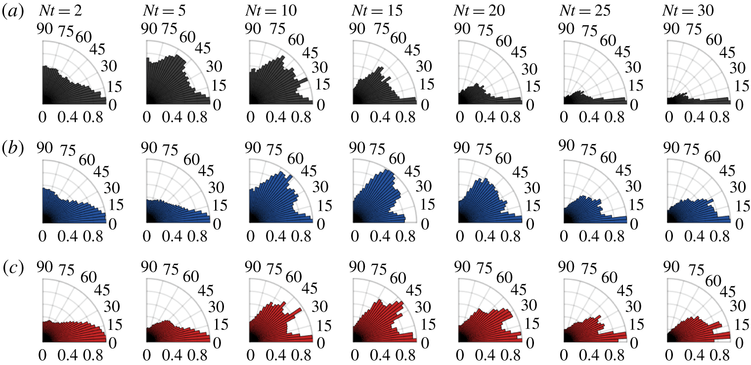
Polar histograms are a convenient means to illustrate the preferred direction of radiated internal waves. In figures 8–10, the radial axis quantifies the normalized mean power flux, while the azimuthal axis enumerates the wave propagation angle relative to the horizontal. Figure 8 shows polar histograms of the mean power flux for the  $Fr=4$ experiments at several snapshots in time. The radiation angles are discretized into bins of 5° and the mean power flux has been normalized by its maximum value at each time. The
 $Re=5\times 10^{3},10^{5}$ and 4 × 10⁵ experiments are shown in (a), (b) and (c), respectively.
Mean power-flux dependence on the radiation angle relative to the horizontal for the  $Fr=4$ experiments at
 $Re=5\times 10^{3}$ (a),
 $Re=10^{5}$ (b) and
 $Re=4\times 10^{5}$ (c). The radial axis quantifies the power flux normalized by the maximum value. The azimuthal axis quantifies the wave propagation angle relative to the horizontal.

At time  $Nt=2$ the wave power flux is significant over a broad range of radiation angles, with a skew towards the horizontal, for all three
 $Re$ considered. While this trend continues at
 $Nt=5$ for the two higher
 $Re$ cases, the wave power flux in the lowest
 $Re$ experiment is more evenly distributed, with a peak between 45° and 60°. By
 $Nt=10$ all three
 $Re$ cases become similar again, with waves radiated out of the wake namely at angles between 20° and 70°, in addition to the non-trivial presence of waves radiated at angles close to the horizontal. The wave power flux has a similar angle distribution for the
 $Re=10^{5}$ and 4 × 10⁵ cases at
 $Nt=15$. However, at the same time in the
 $Re=5\times 10^{3}$ experiment, the contribution at intermediate angles has begun to diminish. From
 $Nt=20$ onward, emitted waves transition towards nearly horizontal radiation angles, a trend which is slowed with increasing
 $Re$. The
 $Re=10^{5}$ experiment reveals waves radiated at angles > 10° which still have non-negligible power at
 $Nt\leqslant 30$. In the highest
 $Re$ case this is true for times
 $Nt<60$ (not shown). At
 $Nt=60$ and all later times (not shown) waves are radiated at nearly horizontal angles regardless of
 $Re$.
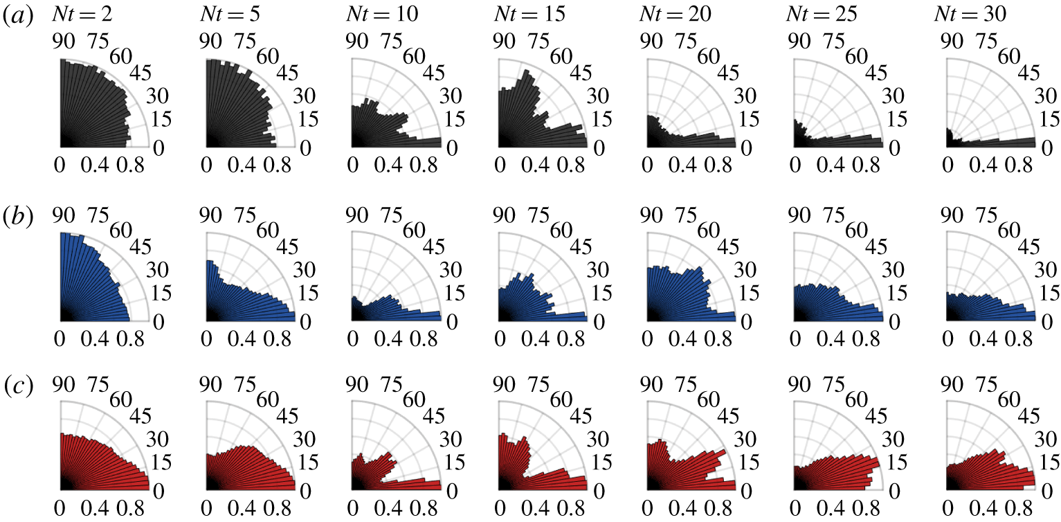
Figure 9 displays the wave power-flux polar histograms for the  $Fr=16$ experiments. Trends observed for the
 $Fr=4$ experiments are also seen here with some slight differences. At early times,
 $Nt\leqslant 5$, waves radiated over a broad range of angles are observed. A significant contribution from waves emitted close to the vertical is seen, most notably for the
 $Re=5\times 10^{3}$ and 105 cases. For all
 $Re$, emitted waves radiate out at intermediate angles between 20° and 70° during
 $10\leqslant Nt\leqslant 15$; however, the power of these waves is reduced from the
 $Fr=4$ experiments (figure 3). After
 $Nt=20$, waves tend towards radiating out near horizontally. Distinct from the
 $Fr=4$ case is a modest contribution from waves radiated close to the vertical in the window
 $20\leqslant Nt\leqslant 30$.
Mean power-flux dependence on the radiation angle relative to the horizontal for the  $Fr=16$ experiments at
 $Re=5\times 10^{3}$ (a),
 $Re=10^{5}$ (b) and
 $Re=4\times 10^{5}$ (c). Axes follow the convention described in the caption of figure 8.

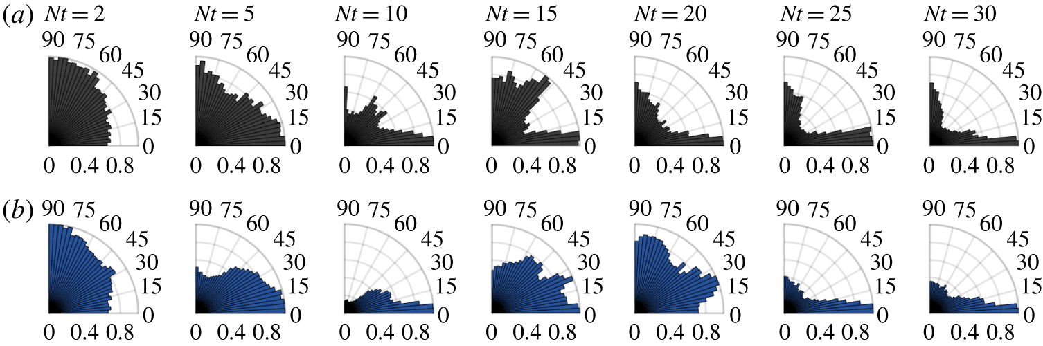
The results of the wave radiation angle analysis for the  $Fr=64$ experiments are shown in figure 10. Trends follow a similar pattern to the
 $Fr=4$ and 16 cases already discussed. A key difference
 $20\leqslant Nt\leqslant 45$, is the contribution from nearly vertically propagating waves in the
 $Re=5\times 10^{3}$ case.
Mean power-flux dependence on the radiation angle relative to the horizontal for the  $Fr=64$ experiments at
 $Re=5\times 10^{3}$ (a) and
 $Re=10^{5}$ (b). Axes follow the convention described in the caption of figure 8.

Finally, it is worth noting the similarity of the above results to those of Maffioli et al. (Reference Maffioli, Davidson, Dalziel and Swaminathan2014). The particular study of a stratified turbulent cloud observed horizontally propagating waves generated via turbulent mixing processes and resultant density intrusions, and waves travelling at an angle of approximately 37° to the horizontal (53° to the vertical) generated by turbulent eddies.
4.4 Internal wave radiation as a sink for kinetic energy
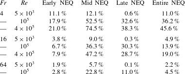
The importance of internal wave radiation in the kinetic energy budget (3.4) remains to be quantified. With this aim, table 2 gives the per cent decrease in total kinetic energy,
 $$\begin{eqnarray}\unicode[STIX]{x0394}{\mathcal{E}}_{k}={\mathcal{E}}_{k}(t_{i})-{\mathcal{E}}_{k}(t_{f}),\end{eqnarray}$$
within the wake-following elliptic cylinder – described in § 3.2 – due to internal wave radiation over four time intervals,  $Nt_{i}\leqslant Nt\leqslant Nt_{f}$ characterizing the NEQ regime: early, mid, late and full regime. Note that for the
 $Re=5\times 10^{3}$ simulations, the third sub-interval of
 $Nt>100$ actually occurs in the Q2D regime (Spedding Reference Spedding1997; Diamessis et al. Reference Diamessis, Spedding and Domaradzki2011).
The per cent decrease in total kinetic energy due to internal wave radiation during the early,  $2\leqslant Nt<10$; mid,
 $10\leqslant Nt\leqslant 100$; late,
 $Nt>100$; and entire NEQ. Note: the last column is not equal to the sum of the previous three columns.

During the early NEQ regime,  $2\leqslant Nt<10$, internal wave radiation makes a marginal contribution to the kinetic energy budget for most experiments: an exception being the two highest
 $Re$ cases with
 $Fr=4$, for which internal wave radiation accounts for approximately a fifth of the decrease in total kinetic energy. In contrast, less than 3 % of the wake kinetic energy lost during this period is lost to internal waves for the
 $Fr=64$ experiments. After the peak wave power flux occurs at
 $Nt=10$, until late in the NEQ regime, wave radiation is responsible for a significant fraction of the kinetic energy lost by the wake in nearly all experiments. In fact, internal wave radiation is the dominant sink for wake energy in the highest
 $Re$ experiment having
 $Fr=4$ – accounting for almost 75 % of the decrease in kinetic energy. In all but the lowest
 $Re$ experiments, internal wave radiation is clearly a non-negligible process during the mid NEQ regime. Late in the wake life cycle,
 $Nt>100$, internal waves are still actively draining energy from the wake for the
 $Fr=4,16$ experiments with
 $Re\geqslant 10^{5}$; in contrast, at low
 $Re$, internal wave radiation is not a significant sink for wake kinetic energy. Finally, the last column of table 2 gives the per cent of wake kinetic energy lost to wave radiation over the entire duration of each experiment. Internal wave radiation is a significant, possibly dominant, sink for wake kinetic energy at
 $Fr=4$ and
 $Re\geqslant 10^{5}$. For experiments with
 $Fr=16$ and
 $Re\geqslant 10^{5}$, internal waves make a non-negligible contribution to the kinetic energy budget; however, another process is most likely the dominant sink for kinetic energy. Wakes having low
 $Re$ or high
 $Fr$ lose relatively little kinetic energy to internal wave radiation.
5 Discussion
Analysis of the energy radiated by internal waves through a wake-following elliptic cylinder revealed the instantaneous wave power radiated from the wake decreases significantly with  $Fr$ at all
 $Re$. A
 $Fr^{-7/3}$ scaling, derived using arguments based on mean wake scales, was found to collapse the volume-averaged wave power time series. For all
 $Re$ considered,
 $Fr$ being equal, a peak in the wave power time series occurs at nearly the same time and has approximately the same magnitude. Therefore, since the peak wave power is the same magnitude in all cases with equivalent
 $Fr$, differences in total wave energy as the
 $Re$ increases must come from late-NEQ contribution of the wave power time series. It can be safely conjectured that this ‘slow-burn’ trend will continue, and is likely to intensify, for higher
 $Re$.
The analysis of far-field wake-radiated internal waves by Zhou & Diamessis (Reference Zhou and Diamessis2016) suggests that the largest amplitude waves are emitted early in the NEQ and that wave amplitude increases with  $Re$. Given the collapse in peak wave power for a fixed
 $Fr$ discussed previously, the difference in amplitude of far-field waves across
 $Re$ can be attributed purely to the decrease in viscous damping of radiated waves (Taylor & Sarkar Reference Taylor and Sarkar2007; Abdilghanie & Diamessis Reference Abdilghanie and Diamessis2013). Zhou & Diamessis (Reference Zhou and Diamessis2016) additionally suggest that the conjecture of Abdilghanie & Diamessis (Reference Abdilghanie and Diamessis2013), that Kelvin–Helmholtz-like instabilities within the interior of the wake are responsible for late-NEQ internal wave radiation, is incorrect based on observation that the most energetic far-field waves are emitted at early times. These two viewpoints are not mutually exclusive and are reconciled presently: indeed the most energetic waves are emitted from the wake early in the NEQ; however, the cumulative contribution of the weak late-NEQ waves, driven by turbulence in the strongly stratified regime, to the wake dynamics is non-negligible.
Linear internal wave theory evinces a clear relationship between the propagation angle of internal waves and their intrinsic frequency (Sutherland Reference Sutherland2011). Using this relationship the frequencies of structures responsible for generating the waves could also be inferred. Unfortunately, the physics are more complicated in the current context due to the presence of a mean flow, i.e. the wake. Waves propagating in a mean flow can be refracted and undergo complex nonlinear interactions: critical reflection and critical-layer absorption (Bühler Reference Bühler2014). In the present study, energetic waves have been found to be emitted over a broad range of angles early in the NEQ regime – similar to the observations of Spedding et al. (Reference Spedding, Browand, Bell and Chen2000). During the period  $10\leqslant Nt\leqslant 25$ wave power flux is less uniformly distributed as a function of radiation angle, clustering between 20° and 70° to the horizontal; however, later in the NEQ regime, radiated energy has been found in near-horizontally emitted waves. It is noteworthy that the theoretical model constructed by Voisin (Reference Voisin1995) predicts that the most energetic waves generated by the wake propagate at an angle of approximately 45° to the horizontal, and hence fall in the range observed here during
 $10\leqslant Nt\leqslant 25$. Similarly, in their laboratory experiments, Brandt & Rottier (Reference Brandt and Rottier2015) observed the most energetic internal waves radiated from a wake to propagate at angles in the range
 $55^{\circ }\leqslant \unicode[STIX]{x1D703}\leqslant 65^{\circ }$. Determining the exact mechanism responsible for the observed wave radiation angles, identifying the dominant wave generation sites within the wake core and periphery, and quantifying the actual propagation angles away from the wake edge into the near and far field, are all topics for further study.
At early times, wave radiation comprises a small fraction of the kinetic energy lost by the wake – an exception being wakes with low  $Fr$ and high
 $Re$ – suggesting other processes such as viscous dissipation or mixing must be the dominant sink for kinetic energy during this period. For all but the low
 $Re$ wakes, internal wave radiation accounts for a significant fraction of wake kinetic energy lost during the mid-NEQ regime (
 $10\leqslant Nt\leqslant 100$): nearly 75 % in the experiment with
 $Fr=4$ and
 $Re=4\times 10^{5}$. Late in the NEQ regime, internal waves continue to drain wake energy for low to moderate
 $Fr$ wakes with
 $Re\geqslant 10^{5}$. Overall, current analysis suggests that internal wave radiation is likely the ultimate or penultimate sink for wake kinetic energy at low
 $Fr$ and high
 $Re$. Note that this is in contrast to the higher
 $Fr$-biased work of Redford et al. (Reference Redford, Lund and Coleman2015), who conclude that internal wave radiation makes a negligible contribution to the overall energy budget; however, it confirms the results of both Brucker & Sarkar (Reference Brucker and Sarkar2010) and Watanabe et al. (Reference Watanabe, Riley, de Bruyn Kops, Diamessis and Zhou2016), who found that the rate of energy loss due to internal wave radiation was comparable to the viscous dissipation of kinetic energy inside the wake core in the early NEQ.
Finally, it was demonstrated in Maffioli, Brethouwer & Lindborg (Reference Maffioli, Brethouwer and Lindborg2016) that the energy lost to mixing is of the same order of magnitude as viscous dissipation for homogeneous turbulence subject to strongly stratified conditions. Investigation of the importance of viscous dissipation and mixing to the wake energy budget, in conjunction with the role of internal wave radiation, should be the focus of future work.
6 Conclusions
The energetics of internal waves radiated from a stratified turbulent wake have been examined using numerical experiments with  $Fr=4$, 16, or 64, and
 $Re=5\times 10^{3}$, 105 or 4 × 10⁵ – the highest Reynolds number experiments being sui generis in the stratified wake literature. Essential, in this regard, is the pointwise calculation of the work performed by perturbation pressure,
 $p^{\prime }\boldsymbol{u}$. To the authors’ best knowledge, this is the first time this quantity has been computed directly and systematically over the full life cycle of a stratified turbulent wake. As a result, the wave power and energy radiated through both a horizontal plane fixed above the wake and a wake-following elliptic cylinder have then been calculated. The latter calculation approach accounts more efficiently for the inhomogeneity of the wake cross-section in both transverse and vertical directions. The resulting non-trivial challenges of interpolation and numerical integration over the elliptic cylinder, which are absent when restricted to the commonly used approach of integrating over a horizontal plane (Taylor & Sarkar Reference Taylor and Sarkar2007; Pham, Sarkar & Brucker Reference Pham, Sarkar and Brucker2009), have been addressed by adopting elements of spectrally accurate quadrature (see appendix A).
The findings of this study are restricted to the near field, i.e. close to the turbulent/non-turbulent interface of the wake. For a fixed  $Fr$, peak wave power occurs at approximately the same time,
 $Nt\approx 10$, with similar magnitude, across all
 $Re$ considered. Wave power continues to be radiated from the wake for much longer times with increasing
 $Re$. Total time-integrated wave energy emitted from the wake increases with
 $Re$ and decreases with
 $Fr$, collapsing to nearly the same value for the
 $Fr=64$ experiments. The most intense internal wave radiation is emitted from the sides, and near the top and bottom of the wake, before
 $Nt\approx 10$. After
 $Nt\approx 10$, radiation of energetic internal waves becomes intermittent around the wake periphery. At early times,
 $Nt<10$, energetic internal waves are found to be emitted over a broad range of angles, though slightly biased towards the horizontal in the
 $Re=10^{5}$ and 4 × 10⁵ experiments. Over the interval
 $10\leqslant Nt\leqslant 25$, a modest trend towards waves travelling at angles between 20° and 70° emerges; however, at late times, a clear trend to nearly horizontally propagating waves is found in all experiments. The percentage of wake kinetic energy lost to internal wave radiation is calculated for the early, mid, and late portions of the non-equilibrium regime of wake evolution. Early NEQ internal wave radiation – before
 $Nt=10$ – comprises only a small fraction of the kinetic energy budget for wakes having
 $Fr\geqslant 16$, and almost 20 % of the energy budget for low
 $Fr$ wakes having
 $Re\geqslant 10^{5}$. Therefore, other processes form the dominant balance in the kinetic energy budget during this period. Wave radiation is a significant sink for wake kinetic energy over the interval
 $10\leqslant Nt\leqslant 100$ in all but the lowest
 $Re$ wakes, accounting for nearly 75 % of the decrease in wake kinetic energy in experiment with
 $Re=4\times 10^{5}$ and
 $Fr=4$. Wave radiation contributes to approximately a third of the wake kinetic energy lost late in the NEQ regime, for wakes having low to moderate initial Froude number and
 $Re\geqslant 10^{5}$. These findings suggest that, although the peak internal wave radiation occurs early in the NEQ regime during the onset of buoyancy control across the actively turbulent near wake, non-negligible wave radiation can occur in subsequent times at sufficiently high
 $Re$. Ultimately internal wave radiation is found to comprise a significant fraction of kinetic energy lost by the wake during the NEQ – over 45 % for a wake having initial
 $Re=4\times 10^{5}$ and
 $Fr=4$.
Confirmation of the results discussed herein for larger initial Reynolds number values is essential for insight into geophysical and ocean engineering applications. A current enterprise – increasing the performance and scalability of the application code used to conduct the numerical experiments described in § 2.3 – promises to capacitate the simulation of stratified wakes with initial Reynold number 2 × 10⁶ and possibly greater. Simulation of higher  $Re$ wakes, concurrent with a more complete energy budget analysis, will be the focus of work in the near future. Additionally, parameter space exploration will be conducted at the
 $Re$ examined in this text to establish whether a critical
 $Fr$ value exists, beyond which a stratified wake can no longer efficiently generate internal waves.
Acknowledgements
The authors are grateful for financial support provided by the US Office of Naval Research (grant N00014-15-1-2513; program managers Dr T. Fu and Dr J. Gorski). The work of the third author is supported, in part, by a Discovery Grant (RGPIN-2018-04329) awarded by the Natural Sciences and Engineering Research Council of Canada (NSERC). All computing resources were provided by the US Department of Defense High Performance Computing Modernization Program (frontier project FP-CFD-FY14-007; principal investigator S. de Bruyn Kops). We would like to thank Professors J. Riley, S. de Bruyn Kops, G. Spedding, K. G. Lamb, M. Stastna and Dr A. Muschinski for discussions which guided and galvanized this work.
Declaration of interests
The authors report no conflict of interest.
Appendix A. Calculation of the fluxes through an elliptic cylinder
Consider an open elliptic cylinder of length  $L$ whose cross-section perpendicular to the
 $x$-axis is given implicitly by the equation
 $$\begin{eqnarray}\frac{y^{2}}{a^{2}}+\frac{z^{2}}{b^{2}}=1.\end{eqnarray}$$
Without loss of generality, we will assume the major axis of the ellipse is parallel to the horizontal – i.e.  $a>b$. In this case the eccentricity is given by
 $$\begin{eqnarray}\unicode[STIX]{x1D716}=\sqrt{1-b^{2}/a^{2}},\end{eqnarray}$$
which is a measure of the aspect ratio of the ellipse. Let  $\unicode[STIX]{x1D6E4}$ be the locus of points in the
 $yz$-plane which satisfy (A 1). The total flux
 $\unicode[STIX]{x1D6F7}$ of a vector field
 $\boldsymbol{F}$ through the surface of the open elliptic cylinder is given by
 $$\begin{eqnarray}\unicode[STIX]{x1D6F7}=\mathop{\oint }_{\unicode[STIX]{x1D6E4}}\mathop{\int }_{0}^{L}\boldsymbol{F}\boldsymbol{\cdot }\hat{\boldsymbol{n}}\,\text{d}x\,\text{d}s,\end{eqnarray}$$
where  $\boldsymbol{n}$ is the outward oriented unit normal vector to
 $\unicode[STIX]{x1D6E4}$. Under some mild assumptions about
 $\boldsymbol{F}$, the integrals can be evaluated in either order and one can choose to evaluate the horizontal integral first,
 $$\begin{eqnarray}\bar{\boldsymbol{F}}=\int _{0}^{L}\boldsymbol{F}\,\text{d}x.\end{eqnarray}$$
If the vector field is periodic in the  $x$-coordinate then this integral can be approximated using spectrally accurate Fourier quadrature on equidistant points via the periodic trapezoid rule (Trefethen Reference Trefethen2000). The remaining line integral
 $$\begin{eqnarray}\unicode[STIX]{x1D6F7}=\oint _{\unicode[STIX]{x1D6E4}}\bar{\boldsymbol{F}}\boldsymbol{\cdot }\hat{\boldsymbol{n}}\,\text{d}s\end{eqnarray}$$
has intrinsically periodic geometry and can also be evaluated using Fourier quadrature.
The end game of the current development is a highly accurate quadrature approximation to  $\unicode[STIX]{x1D6F7}$ given in (A 3) using the values of a vector field
 $\boldsymbol{F}$ obtained from numerical experiments conducted on Cartesian mesh
 $(x_{i},y_{j},z_{k})$,
 $1\leqslant i\leqslant N_{x}$,
 $1\leqslant j\leqslant N_{y}$,
 $1\leqslant k\leqslant N_{z}$. The value of the total flux is independent of the parameterization of
 $\unicode[STIX]{x1D6E4}$ used to evaluate the line integral. A trivial parameterization of the ellipse is given by
 $$\begin{eqnarray}y=a\cos \unicode[STIX]{x1D703}\quad z=b\sin \unicode[STIX]{x1D703},\end{eqnarray}$$
where  $\unicode[STIX]{x1D703}$ is the azimuthal angle made with the positive
 $y$-axis; however, for a highly eccentric ellipse (
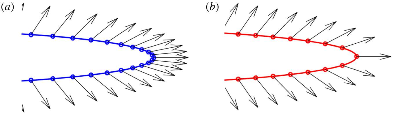
 $\unicode[STIX]{x1D716}\gg 0$) the corresponding equiangular quadrature points cluster tightly at the edges of the ellipse as seen in figure 11. In the analysis of internal waves radiated from a wake, the total flux of a vector field with significant horizontal variation through a highly eccentric ellipse will be calculated – consequently, a very large number of quadrature points would be necessary to obtain an accurate approximation. A more robust choice is to parameterize the ellipse using arc length. From the first parameterization, the arc length of the path traced anticlockwise from
 $(a,0)$ to
 $(y(\unicode[STIX]{x1D703}),z(\unicode[STIX]{x1D703}))$ on the ellipse can be calculated by
 $$\begin{eqnarray}s=\int _{0}^{\unicode[STIX]{x1D703}}\sqrt{a^{2}\cos ^{2}(\unicode[STIX]{x1D717})+b^{2}\sin (\unicode[STIX]{x1D717})}\,\text{d}\unicode[STIX]{x1D717}=a\int _{0}^{\unicode[STIX]{x1D703}}\sqrt{1-\unicode[STIX]{x1D716}^{2}\sin ^{2}(\unicode[STIX]{x1D717})}\,\text{d}\unicode[STIX]{x1D717}.\end{eqnarray}$$
The connoisseur will recognize this as an incomplete elliptic integral of the second kind, denoted  $E(\unicode[STIX]{x1D703},\unicode[STIX]{x1D716})$ (Abramowitz & Stegun. Reference Abramowitz and Stegun.1972). It follows that the circumference of the ellipse is
 $C=E(2\unicode[STIX]{x03C0};\unicode[STIX]{x1D716})$.
Equiangular points (a) and equidistant points (b) on the ellipse.

The complete algorithm for calculating the flux through an ellipse using  $N_{s}$ equidistant quadrature points is:
(i) Construct a uniform grid
 $s_{r}\in [0,C]$, $1\leqslant r\leqslant N_{s}$.
(ii) Calculate
$\unicode[STIX]{x1D703}_{r}=\text{E}^{-1}(s_{r};\unicode[STIX]{x1D716})$.(iii) Evaluate
$y_{r}^{e}=a\cos \unicode[STIX]{x1D703}_{r}$, $z_{r}^{e}=b\sin \unicode[STIX]{x1D703}_{r}$.(iv) Find
$\bar{\boldsymbol{F}}(y_{j},z_{k})$ via integral (A 4).(v) Determine
$\bar{\boldsymbol{F}}_{r}^{e}=\bar{\boldsymbol{F}}(y_{r}^{e},z_{r}^{e})$.(vi) Calculate the flux
$\unicode[STIX]{x1D6F7}$ using (A 5).


A procedure is needed to evaluate both  $E(\unicode[STIX]{x1D703};\unicode[STIX]{x1D716})$ and
 $E^{-1}(s;\unicode[STIX]{x1D716})$. The first is accurately computed using Fourier quadrature in
 $\unicode[STIX]{x1D703}$, while second can be evaluated using the iterative method given in Boyd (Reference Boyd2012). The value of the vector field
 $\bar{\boldsymbol{F}}$ is found using interpolation from the simulation grid points
 $(y_{j},z_{k})$, to the elliptic quadrature points
 $(y_{r}^{e},z_{r}^{e})$. Denote this operation as
 ${\mathcal{I}}_{r}:\mathbb{R}^{2}\rightarrow \unicode[STIX]{x1D6E4}$:
 $$\begin{eqnarray}\bar{\boldsymbol{F}}_{r}^{e}={\mathcal{I}}_{r}\bar{\boldsymbol{F}}(y_{j},z_{k}).\end{eqnarray}$$
In particular, the computational grid used for the numerical experiments presented in this work utilizes equally spaced Fourier collocation points in the horizontal and Gauss–Legendre–Lobatto collocation points within each vertical subdomain. Interpolation onto the ellipse is conducted using band-limited sinc functions in the horizontal and barycentric Lagrange interpolation within the particular vertical subdomain containing  $z_{r}^{e}$. Finally, the Fourier quadrature weights on an interval
 $[0,l]$ using
 $N$ points are all equal and given by
 $\unicode[STIX]{x1D714}=l/N$; therefore, the ultimate expression for the numerical approximation of the flux given in (A 3) is
 $$\begin{eqnarray}\unicode[STIX]{x1D6F7}=\frac{C}{N_{s}}\frac{L}{N_{x}}\mathop{\sum }_{r=1}^{N_{\unicode[STIX]{x1D703}}}{\mathcal{I}}_{r}\mathop{\sum }_{i=1}^{N_{x}}\boldsymbol{F}(x_{i},y_{j},z_{k}).\end{eqnarray}$$
Diligent pupils of real analysis have likely noted that the result invoked previously to allow for the integration in  $x$ to be conducted first in the expression (A 3) is not guaranteed to hold in the case of discrete quadratures: interpolation and quadrature operations do not necessarily commute. Both orders integration were tested in the evaluation of the total flux and it was found that their results agreed to machine precision. The form of (A 3) in which the
 $x$ integral is evaluated first is advantageous as it only requires one interpolation operation (A 8) instead of
 $N_{x}$ interpolations.