1 Introduction
Deformation of an erodible substrate into large-scale bedforms such as dunes, makes understanding turbulence transport in aeolian, fluvial and marine environments complex (Fourrière, Claudin & Andreotti Reference Fourrière, Claudin and Andreotti2010). While the transport of erodible sand or gravel is a function of instantaneous forces or their time integrated effect (impulse), the development of bedforms affects the spatial distribution of such forces, feeding back into the potential for further erosion to take place (Jackson Reference Jackson1976; Best Reference Best2005). Dunes are observed, and are deemed of significance to the dynamics of near-surface boundary layers in various planetary environments (Titus, Zimbelman & Radebaugh Reference Titus, Zimbelman and Radebaugh2015). As a consequence, there have been extensive field studies of flow over such features in aeolian (Lancaster et al. Reference Lancaster, Nickling, Neuman and Wyatt1996; Wiggs, Livingstone & Warren Reference Wiggs, Livingstone and Warren1996) and fluvial or marine environments (Kostaschuk & Villard Reference Kostaschuk and Villard1996; Osborne & Rooker Reference Osborne and Rooker1999; Kostaschuk Reference Kostaschuk2000; Shugar et al. Reference Shugar, Kostaschuk, Best, Parsons, Lane, Orfeo and Hardy2010) as well as many experimental studies (Nelson, McLean & Wolfe Reference Nelson, McLean and Wolfe1993; Bennett & Best Reference Bennett and Best1995; Venditti & Bennett Reference Venditti and Bennett2000; Dumas, Arnott & Southard Reference Dumas, Arnott and Southard2005).
While there are also examples of older numerical studies studying the flow structure in these environments (Salvetti, Damiani & Beuxm Reference Salvetti, Damiani and Beuxm2001; Parsons, Walker & Wiggs Reference Parsons, Walker and Wiggs2004), it is only recently that high-resolution eddy-resolving numerical studies have been performed (Zedler & Street Reference Zedler and Street2001; Stoesser et al. Reference Stoesser, Braun, Garcia-Villalba and Rodi2008) and flow structure generation mechanisms have been considered using numerical models (Omidyeganeh & Piomelli Reference Omidyeganeh and Piomelli2011, Reference Omidyeganeh and Piomelli2013a ,Reference Omidyeganeh and Piomelli b ; Chang & Constantinescu Reference Chang and Constantinescu2013). In the context of the two-dimensional dunes that have tended to form the emphasis of previous experimental work (Bennett & Best Reference Bennett and Best1995; Venditti & Bennett Reference Venditti and Bennett2000; Stoesser et al. Reference Stoesser, Braun, Garcia-Villalba and Rodi2008; Omidyeganeh & Piomelli Reference Omidyeganeh and Piomelli2011; Chang & Constantinescu Reference Chang and Constantinescu2013), recent work has focused on the generation mechanisms describing the large-scale hairpin features in such flows, with a variety of mechanisms proposed:
-
(i) Stoesser et al. (Reference Stoesser, Braun, Garcia-Villalba and Rodi2008) suggested that these structures are produced close to reattachment of the separated shear layer (SSL) that is generated close to the dune crest;
-
(ii) Omidyeganeh & Piomelli (Reference Omidyeganeh and Piomelli2011) focused on the vortex tubes associated with the Kelvin–Helmholtz vortices that are produced in the SSL. They found that the hairpins were a consequence of disturbances to these structures owing to the presence of other structures in the outer part of the dune flow;
-
(iii) Chang & Constantinescu (Reference Chang and Constantinescu2013) examined this looking not only at a fully developed flow with periodic boundary conditions, but also at spatially developing transitional flow where the subdued activity of the smaller scales made identification of the mechanism responsible for the formation of the large-scale coherent structures much clearer. They found that the vortex tube induced by the dune upstream is transported above the SSL of the dune downstream, giving it a greater mean velocity while retaining more coherence. As the upstream tube passes (and perhaps touches) the tube in the SSL, significant distortion results, leading to the observed hairpin structures that scaled with dune size.
Hence, there are some similarities here to the generation of much smaller hairpin structures in the boundary layer (Robinson Reference Robinson1991; Christensen & Adrian Reference Christensen and Adrian2001; Ganapathisubramani, Longmire & Marusic Reference Ganapathisubramani, Longmire and Marusic2003) in terms of velocity gradients inducing lift-off and distortion of tubes of vorticity. However, the pre-existence of a SSL, and the association with fixed spatial positions (dune crests), rather than a spatially pseudo-random autogeneration, means that the integrated effect on the velocity structure at a particular location is likely to be very different. In addition to the large-scale hairpins, other types of large-scale coherent structures are present in flow over large-scale roughness, including ‘superstreaks’, that scale with the size of roughness elements, and kolks. These kolk vortices form when the large-scale hairpins interact with the flow field of the dunes downstream (Babakaiff & Hickin Reference Babakaiff, Hickin, Ashworth, Bennett, Best and McLelland1996; Grigoriadis, Balaras & Dimas Reference Grigoriadis, Balaras and Dimas2009).
One means of characterising this structure is in terms of the relation between velocity and intermittency and, recently, it has been shown that the outer part of flow over bedforms has a different coupling between the longitudinal velocity component,
 $u_{1}$
, and the intermittency in the dynamics of this signal (Keylock, Singh & Foufoula-Georgiou Reference Keylock, Singh and Foufoula-Georgiou2013), compared to the structure of boundary-layer flows, jets and wakes. This result has been confirmed by Keylock et al. (Reference Keylock, Singh, Venditti and Foufoula-Georgiou2014b
) for a dune flow dataset collected under very different experimental conditions (various measuring positions about fixed dunes as opposed to one measuring position and mobile bedforms advected beneath the probe). While the previous experimental studies were able to resolve consistent information on the nature of the velocity-intermittency structure in the outer part of a flow over bedforms, the experimental design for those studies meant that limited information was available beneath the dune crest (the inner flow region). In order to gain an insight into the flow structure in this region, this study uses large eddy simulation (LES) (Sagaut Reference Sagaut2002; Geurts Reference Geurts2003) to study the flow over sinusoidal bedforms. The simulation provides additional insights into the velocity-intermittency structure of turbulent flow over bedforms, particularly in the near-wall region. In addition, the ability to explain the velocity-intermittency results in terms of the resolved coherent flow structures demonstrates the effectiveness of our quadrant method (Keylock, Nishimura & Peinke Reference Keylock, Nishimura and Peinke2012) for capturing flow structure information from single-point single velocity component data.
The paper is organised as follows: first, we describe the numerical domain and properties of the numerical simulation, as well as validation of the code against previous experimental and numerical studies. Second, we explain the background to, and specific calculation procedure for, the velocity-intermittency analysis. The methods section concludes with an explanation of the data clustering/classification technique used to group the 2048 time series analysed into discrete categories. The results section describes vertical profiles of mean velocity and turbulence quantities before examining the correlation between velocity and intermittency at various locations in the flow domain. These correlations are then disaggregated using our quadrant methodology to reveal greater structure to the flow than the correlations imply. The velocity-intermittency structure of the outer and inner regions are then described and linked to the nature of the flow structure at these respective locations using information from instantaneous vorticity fields.
2 Methods
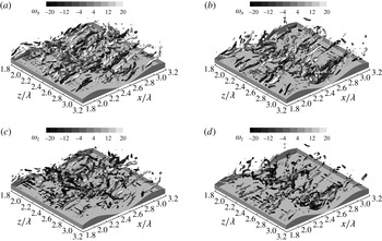
2.1 Numerical methods and flow domain
The numerical simulations were undertaken using a non-dissipative, parallel, finite-volume LES code (Pierce & Moin Reference Pierce and Moin2001), which solves the incompressible Navier–Stokes equations on a non-uniform Cartesian mesh. The fractional step algorithm uses a staggered conservative space–time discretization with a semi-implicit iterative method to advance the equations in time. The algorithm is second-order accurate in both space and time. The numerical method discretely conserves energy (Mahesh, Constantinescu & Moin Reference Mahesh, Constantinescu and Moin2004) and uses strictly non-dissipative (central) discretizations to solve for the momentum and pressure. The subfilter-scale viscosity in the viscous terms is calculated dynamically from the resolved velocity fields (Germano Reference Germano1992; Pierce & Moin Reference Pierce and Moin2001). The flow was driven by imposing the mass flow rate, and the boundary condition at the free surface was a slip-symmetry condition, where the normal velocity component and the vertical derivatives of the horizontal velocity components were set to zero (
 $\unicode[STIX]{x2202}u_{1}/\unicode[STIX]{x2202}y=\unicode[STIX]{x2202}u_{3}/\unicode[STIX]{x2202}y=0$
). The dunes were represented with a stair-step approximation, with no slip on each element of the dune surface.
Additional details concerning the numerical method, as well as validation studies, are given in Chang, Constantinescu & Park (Reference Chang, Constantinescu and Park2006, Reference Chang, Constantinescu and Park2007), Chang & Constantinescu (Reference Chang and Constantinescu2013, Reference Chang and Constantinescu2015). Grid convergence work was undertaken to underpin the mesh design in those studies. However, it should be emphasized that because of the need to obtain physically meaningful Hölder exponents from the numerical model, which is a more stringent requirement than the appropriate resolution of large-scale flow structures, the present study was undertaken on a much finer numerical mesh than these past studies. Indeed, the mesh for the current study was six times finer than in the simulations reported by Chang & Constantinescu (Reference Chang and Constantinescu2013) at 5 wall units (and vertically, 2.5 units in the dune region). Hence, the first mesh point is within the viscous sublayer, removing the need for wall functions, and dramatically reducing any dependence on the subgrid model physics. Furthermore, the mesh refinement used in the present study was close to that required by direct numerical simulation (DNS) at the same channel Reynolds number. Hence, because the subgrid-scale viscosity from the dynamic Smagorinsky model goes to zero in regions where the resolution approaches that for a well-resolved DNS, this provides another means by which the simulation’s dependence on subgrid-scale physics is reduced. Analysis of the instantaneous and mean-flow fields confirmed the small values of the non-dimensional subgrid-scale viscosity (
 $\unicode[STIX]{x1D708}_{SGS}/\unicode[STIX]{x1D708}<0.05$
) outside of the regions containing larger-scale turbulent eddies (separated shear layers and in the troughs of the dunes). In the latter regions, the maximum instantaneous values of
 $\unicode[STIX]{x1D708}_{SGS}/\unicode[STIX]{x1D708}$
were close to 1.2, while the maximum time-averaged values were close to 0.5.
The computational domain and the numerical mesh employed. Note that the origin for
 $y$
in this study is at the midheight of the bedform.

Properties of the flow domain and the mesh for the numerical experiment. The channel height,
 $h_{c}$
, and inlet depth-averaged mean velocity,
 $U$
, were both equal to 1 and the mesh sizes
 $\unicode[STIX]{x1D6E5}_{x,y,z}$
are non-dimensionalised with respect to
 $h_{c}$
.

The numerical domain is shown in figure 1 and relevant properties, including the number of computational cells used in each direction,
 $N_{x,y,z}^{L}$
, and their size,
 $\unicode[STIX]{x1D6E5}_{x,y,z}$
, are given in table 1. Because the large-scale ‘super-streak’ structures have a streamwise extent greater than that for one dune (Kruse, Günther & von Rohr Reference Kruse, Günther and von Rohr2003), to capture such structures accurately in a simulation with periodic boundary conditions requires a domain at least three times the length of this structure so that periodic constraints do not impact on the inferred dynamics of the vortices. Hence, the computational domain here, spanning four dune wavelengths, exceeds that in most previous studies. The particular bedforms used in this study were motivated by the work of Günther & von Rohr (Reference Günther and von Rohr2003). Such symmetrical dunes arise in nature when a mobile bed is subject to an oscillating flow, as occurs in tidal environments. The geometry of the bedforms is stated in table 1. Within the computational domain, time series were extracted from 2048 positions, corresponding to the 32 positions shown in figure 2(a), replicated over all four bedforms, for 16 values of the transverse coordinate,
 $z/\unicode[STIX]{x1D706}\in \{1.0,1.5,2.0,2.3,2.4,2.425,2.45,2.5,2.525,2.55,2.6,2.7,3.0,3.5,4.0,4.5\}$
. The time series were of a 200
 $h_{c}/U$
duration and sampled every
 $(1/30)h_{c}/U$
, where
 $U$
is the temporally and spatially averaged mean flow at the inlet to the domain. The data were obtained after a period of convergence and it was checked that they were stationary from the perspective of the key term needed for our analysis method (the Hölder exponents,
 $\unicode[STIX]{x1D6FC}_{1}$
described in § 2.3.1). To demonstrate this, we show the time series for
 $\unicode[STIX]{x1D6FC}_{1}$
for all 32 locations in a given
 $x$
–
 $y$
plane for a single dune in figure 3. It is clear that the data are stationary in their mean, implying a stationary variance to the velocity time series,
 $u_{1}$
.
The 32 sampling locations employed for all 16 values for the transverse coordinate,
 $z$
, and for all four dunes are shown in (a). These points are superimposed on a frame showing the instantaneous spanwise vorticity,
 $\unicode[STIX]{x1D714}_{z}$
for flow over and about the fourth and fifth dunes, with colouring respecting the key for that panel. (b) Shows a portion of the flow domain at one instance of time. The magnitude of the total vorticity on an
 $x$
–
 $y$
plane in the centre of the domain is highlighted, with three-dimensional coherent structures resolved using the Q-criterion (Hunt, Wray & Moin Reference Hunt, Wray and Moin1988) throughout the domain.

Time series showing the stationarity of the Hölder exponents,
 $\unicode[STIX]{x1D6FC}_{1}$
for the 32 sampling locations shown in figure 2(a). From top to bottom we commence with
 $x/\unicode[STIX]{x1D706}=\unicode[STIX]{x1D712}.00$
,
 $y/\unicode[STIX]{x1D706}=0.06$
, work along increasing
 $y$
and then move to the next
 $x/\unicode[STIX]{x1D706}$
position, finishing at
 $x/\unicode[STIX]{x1D706}=\unicode[STIX]{x1D712}.75$
,
 $y/\unicode[STIX]{x1D706}=0.9$
. Each series is displaced vertically by an integer value for clarity.

2.2 Validation of the LES with experiments and DNS
The LES code has been validated for a wide range of turbulent flows including channel flow over dunes. The reader is referred to Chang & Constantinescu (Reference Chang and Constantinescu2013) for a detailed comparison between LES, experiment and DNS for flow in a channel with dunes at the bottom and a no-slip boundary condition at the top of the domain based on a coarser mesh than adopted here. For example, figure 4 compares the vertical velocity profiles obtained at two longitudinal positions (the dune crest,
 $x/\unicode[STIX]{x1D706}=0.0$
, and the point of minimum elevation,
 $x/\unicode[STIX]{x1D706}=0.5$
) for an inflow Reynolds number (flow depth and depth-averaged mean velocity) of 6700, which matched that in the experiments of Günther & von Rohr (Reference Günther and von Rohr2003). Higher-order statistical quantities (the root-mean-squared velocity,
 $\unicode[STIX]{x1D70E}(u_{1})$
, and the Reynolds stresses,
 $-\langle u_{1}^{\prime }u_{2}^{\prime }\rangle$
) are compared to a DNS at a Reynolds number of 6920 by Cherukat, Na & Hanratty (Reference Cherukat, Na and Hanratty1998) in figure 5. It should be noted that this DNS was conducted in a fairly narrow channel and the super streaks over the dunes were not resolved. These super-streak features were resolved with the original LES by Chang & Constantinescu (Reference Chang and Constantinescu2013) as well as in the current study with a much finer mesh as is clear in figure 2 and in the instantaneous fields shown towards the end of this paper.
Comparisons of vertical profiles of the
 $u_{1}$
velocity component at
 $x/\unicode[STIX]{x1D706}=0.0$
and
 $x/\unicode[STIX]{x1D706}=0.5$
predicted by the LES simulation and measured with two different experimental techniques: laser Doppler velocimetry (Hudson, Dykhno & Hanratty Reference Hudson, Dykhno and Hanratty1996) and particle imaging velocimetry (Günther & von Rohr Reference Günther and von Rohr2003). This figure is taken from Chang & Constantinescu (Reference Chang and Constantinescu2013), (copyright American Geophysical Union) and is reproduced with the permission of the AGU.

Comparisons of vertical profiles of
 $\unicode[STIX]{x1D70E}(u_{1})$
(a,c,e) and the Reynolds stresses (b,d,f) obtained at three longitudinal locations (
 $x/\unicode[STIX]{x1D706}\in \{0.0,0.4,0.8\}$
) using a LES simulation for flow over dunes conducted in the same domain as this study and a DNS direct numerical simulation by Cherukat et al. (Reference Cherukat, Na and Hanratty1998).

2.3 Velocity-intermittency analysis
The intermittency of turbulence has long been recognized, resulting in the various forms for the corrections to Kolmogorov’s original (K41) (Kolmogorov Reference Kolmogorov1941) structure function scaling (Kolmogorov Reference Kolmogorov1962; Frisch, Sulem & Nelkin Reference Frisch, Sulem and Nelkin1978; She & Leveque Reference She and Leveque1994), and explicit consideration of multifractal approaches (Meneveau & Sreenivasan Reference Meneveau and Sreenivasan1991; Muzy, Bacry & Arnéodo Reference Muzy, Bacry and Arnéodo1991). However, as a consequence of scale-separation arguments (Richardson Reference Richardson1922), the formal links between velocity difference distributions, intermittency and their possible correlations with the velocity field have received less attention (although note that Kolmogorov permits the values for the coefficients in his revised theory to be a function of the macrostructure of the flow (Kolmogorov Reference Kolmogorov1962) and it is suggested by Frisch, Bec & Aurell (Reference Frisch, Bec and Aurell2005) that Kolmogorov recognised this issue in 1941 but ignored it at the time to facilitate the derivation of the
 $4/5$
law).
In terms of experimental and theoretical investigation into these matters, the relation between the longitudinal velocity difference, over a length,
 $r$
, given by
 $\unicode[STIX]{x0394}u_{r}=u_{x}-u_{x+r}$
and
 $u_{x}$
was studied by Praskovsky et al. (Reference Praskovsky, Gledzer, Karyakin and Zhou1993) who demonstrated the invalidity of the sweeping decorrelation hypothesis. More recently, Hosokawa (Reference Hosokawa2007) showed a dependence between velocity increments and the local velocity sum that was broadly consistent with the conclusion of Praskovsky et al. (Reference Praskovsky, Gledzer, Karyakin and Zhou1993). Further work on velocity dependence can be seen in studies that move away from considering the velocity increment moments (structure functions) to studying a Fokker–Planck equation for the evolution of the probability density function of the increments (Renner, Peinke & Friedrich Reference Renner, Peinke and Friedrich2001; Keylock, Stresing & Peinke Reference Keylock, Stresing and Peinke2015). By further conditioning the distribution for
 $p(\unicode[STIX]{x0394}u_{r}|\unicode[STIX]{x0394}u_{2r})$
on the velocity, i.e.
 $p(\unicode[STIX]{x0394}u_{r}|\unicode[STIX]{x0394}u_{2r},u_{x})$
, Stresing & Peinke (Reference Stresing and Peinke2010) were able to show the relevance of describing the turbulent energy cascade with a velocity conditioning.
While this conditional distribution function technique is suited to the analysis of long experimental datasets consisting of millions of samples, it is much less appropriate for studying velocity-intermittency properties derived from eddy-resolving numerical studies or shorter duration geophysical field studies. This deficiency of the Fokker–Planck approach was the rationale for the development of a velocity-intermittency analysis framework better suited to the study of shorter duration time series (Keylock et al. Reference Keylock, Nishimura and Peinke2012). This method is adopted in this paper and explained more thoroughly below. In addition to its links to fundamental questions regarding turbulence cascades and dynamics, this analysis permits an implicit consideration of the role of flow structures in the dynamics from single-point time series (from which the velocity gradient tensor cannot be resolved). Hence, identification of the velocity-intermittency structure complements more conventional analysis of turbulent kinetic energy and Reynolds stresses for single-point data by giving information that one can connect to resolved flow structures (Keylock et al. Reference Keylock, Singh, Venditti and Foufoula-Georgiou2014b ).
2.3.1 Hölder exponents
Similar to multifractal analyses (Meneveau & Sreenivasan Reference Meneveau and Sreenivasan1991), our velocity-intermittency approach is underpinned by the notion of Hölder exponents. The Hölder exponents for a turbulence velocity time series can be used to identify flow structures from single-point measurements (Keylock Reference Keylock2008) and can be formally related to more classical structure function analysis using the Frisch–Parisi conjecture (Frisch & Parisi Reference Frisch, Parisi, Ghil, Benzi and Parisi1985):
 $$\begin{eqnarray}D(\unicode[STIX]{x1D6FC}_{1})=\min _{n}(\unicode[STIX]{x1D6FC}_{1}(t)n-\unicode[STIX]{x1D709}_{n}+1),\end{eqnarray}$$
where the singularity (multifractal) spectrum,
 $D(\unicode[STIX]{x1D6FC}_{1})$
, is given by the set of non-empty values for
 $\unicode[STIX]{x1D6FC}_{1}(t)$
, the Hölder exponents for velocity component
 $u_{1}$
and
 $\unicode[STIX]{x1D709}_{n}$
is the structure function scaling exponent for the
 $n$
th moment of the velocity increment distribution. Hence, analysis in terms of the Hölder regularity of the velocity signal provides a direct connection to considerations of turbulent intermittency (Kolmogorov Reference Kolmogorov1962) and the multifractal structure of turbulent velocity signals (Meneveau & Sreenivasan Reference Meneveau and Sreenivasan1991; Muzy et al.
Reference Muzy, Bacry and Arnéodo1991; Arnéodo et al.
Reference Arnéodo, Manneville, Muzy and Roux1999).
The Hölder exponent is defined through consideration of the differentiability of a signal relative to polynomial approximations about a particular point (Jaffard Reference Jaffard1997; Kolwankar & Lévy Véhel Reference Kolwankar and Lévy Véhel2002). These are given by a Taylor series expansion:
 $$\begin{eqnarray}p_{T}(t)=\mathop{\sum }_{i=0}^{m-1}\frac{u_{1}^{i}(T)}{i!}(t-T)^{i},\end{eqnarray}$$
where we study a velocity time series,
 $u_{1}(t)$
, in a neighbourhood,
 $\unicode[STIX]{x1D6FF}$
, about a position
 $T$
and
 $m$
is the number of times that
 $u$
is differentiable in
 $T\pm \unicode[STIX]{x1D6FF}$
. We then state that
 $u_{1}(t)$
has a pointwise Hölder exponent,
 $\unicode[STIX]{x1D6FC}_{1}\equiv \unicode[STIX]{x1D6FC}(u_{1})\geqslant 0$
if a constant
 $K>0$
and the polynomial
 $p_{T}(t)$
of degree
 $m$
exist such that
 $$\begin{eqnarray}|u_{1}(t)-p_{T}(t)|\leqslant K|t-T|^{\unicode[STIX]{x1D6FD}}.\end{eqnarray}$$
The Hölder regularity,
 $\unicode[STIX]{x1D6FC}_{1}$
, of
 $u_{1}(t)$
at
 $T$
is then given by the supremum of
 $\unicode[STIX]{x1D6FD}$
that fulfils (2.3).
We evaluate
 $\unicode[STIX]{x1D6FC}_{1}$
using a time domain scaling method (Kolwankar & Lévy Véhel Reference Kolwankar and Lévy Véhel2002; Seuret & Lévy Véhel Reference Seuret and Lévy Véhel2003). This method performed well in a comparative test of various such algorithms (Keylock Reference Keylock2010) and is based on the determination of the oscillations within the vicinity of a particular target position and then a log–log regression of these signal oscillations,
 $O_{T\pm \unicode[STIX]{x1D6FF}}$
, within some distance
 $\unicode[STIX]{x1D6FF}$
of
 $T$
against
 $\unicode[STIX]{x1D6FF}$
, where
 $O_{T\pm \unicode[STIX]{x1D6FF}}$
is given by:
 $$\begin{eqnarray}O_{T\pm \unicode[STIX]{x1D6FF}}=\max [u_{1}(t\in \{T-\unicode[STIX]{x1D6FF},\ldots ,T+\unicode[STIX]{x1D6FF}\})]-\min [u_{1}(t\in \{T-\unicode[STIX]{x1D6FF},\ldots ,T+\unicode[STIX]{x1D6FF}\})]\end{eqnarray}$$
and
 $\unicode[STIX]{x1D6FF}$
is distributed logarithmically. In our study
 $2^{1}\leqslant \unicode[STIX]{x1D6FF}\leqslant 2^{10}$
to provide as broad a scaling regime as possible (i.e. spanning integral and inertial scales) to incorporate both dune flow turbulent macrostructure (Kruse et al.
Reference Kruse, Günther and von Rohr2003; Chang & Constantinescu Reference Chang and Constantinescu2013) and cascade effects while minimizing algorithm end-effect issues (our time series each consist of 6000 values).
2.3.2 Velocity-intermittency quadrants
The approach we use for determining the velocity-intermittency coupling is based on the notion of quadrants, commonly used to characterise boundary-layer flows (Nakagawa & Nezu Reference Nakagawa and Nezu1977; Bogard & Tiederman Reference Bogard and Tiederman1986; Keylock, Lane & Richards Reference Keylock, Lane and Richards2014a
). However, in our formulation, the fluctuating vertical velocity component,
 $u_{3}^{\prime }(t)$
is replaced by the fluctuating pointwise Hölder regularity,
 $\unicode[STIX]{x1D6FC}_{1}^{\prime }(t)$
of the fluctuating longitudinal component,
 $u_{1}^{\prime }(t)$
(Keylock et al.
Reference Keylock, Nishimura and Peinke2012). Hence, having obtained
 $\unicode[STIX]{x1D6FC}_{1}(t)$
from
 $u_{1}(t)$
, we form quadrants by subtracting the respective mean values,
 $\unicode[STIX]{x1D6FC}_{1}^{\prime }(t)\equiv \unicode[STIX]{x1D6FC}_{1}(t)-\langle \unicode[STIX]{x1D6FC}_{1}\rangle$
,
 $u_{1}^{\prime }(t)\equiv u_{1}(t)-\langle u_{1}\rangle$
and then classifying the data based on the sign of the fluctuating terms (table 2).
Joint probability distributions of the velocity intermittency in the space used to define the quadrants used in this paper. Data are from the centreline of the domain (
 $z/\unicode[STIX]{x1D706}=2.5$
) and are averaged over the four dunes studied at locations (
 $x/\unicode[STIX]{x1D706}=\unicode[STIX]{x1D712}.00$
,
 $y\unicode[STIX]{x1D706}=0.90$
; (a)); (
 $x/\unicode[STIX]{x1D706}=\unicode[STIX]{x1D712}.50$
,
 $y\unicode[STIX]{x1D706}=0.04$
; (b)); (
 $x/\unicode[STIX]{x1D706}=\unicode[STIX]{x1D712}.00$
,
 $y\unicode[STIX]{x1D706}=0.06$
; (c)); and, (
 $x/\unicode[STIX]{x1D706}=\unicode[STIX]{x1D712}.50$
,
 $y\unicode[STIX]{x1D706}=-0.02$
; (d)). Contours are shown in 0.2 % intervals commencing at 0.2 %. The origin is displayed with a black dotted line, while two example integer hole sizes,
 $\text{H}\in \{1,2\}$
, are shown with grey dotted lines.

Definition of velocity-intermittency quadrants.

To illustrate the method more clearly, we show velocity-intermittency quadrant plots from four selected positions in our numerical domain, combining data from all four dunes, in figure 6. We follow the idea in classical quadrant analysis of identifying selected events (ejections and sweeps in the standard analysis) based on a threshold ‘hole size’. Because the units of measurement for our variables differ, we normalise using the respective standard deviations,
 $\unicode[STIX]{x1D70E}(\ldots )$
:
 $$\begin{eqnarray}\left.\begin{array}{@{}c@{}}\displaystyle \unicode[STIX]{x1D6FC}_{1}^{\prime \ast }(t)=\frac{\unicode[STIX]{x1D6FC}_{1}^{\prime }(t)}{\unicode[STIX]{x1D70E}(\unicode[STIX]{x1D6FC}_{1})}\\ \displaystyle u_{1}^{\prime \ast }(t)=\frac{u_{1}^{\prime }(t)}{\unicode[STIX]{x1D70E}(u_{1})}.\end{array}\right\}\end{eqnarray}$$
We then define our hole size,
 $\text{H}$
, as the value for the product,
 $\unicode[STIX]{x1D6FC}_{1}^{\prime \ast }(t)u_{1}^{\prime \ast }(t)$
, and example thresholds are shown in figure 6 for
 $\text{H}\in \{1,2\}$
as grey dotted lines. The four locations chosen in figure 6 can be seen from figure 2 to represent very different local flow environments:
-
(i) (
 $x/\unicode[STIX]{x1D706}=\unicode[STIX]{x1D712}.00,y\unicode[STIX]{x1D706}=0.90$
) – the outer flow far above the dunes (a);
-
(ii) (
$x/\unicode[STIX]{x1D706}=\unicode[STIX]{x1D712}.50,y\unicode[STIX]{x1D706}=0.04$
) – within the shear layer formed by separation at the upstream crest (b); -
(iii) (
$x/\unicode[STIX]{x1D706}=\unicode[STIX]{x1D712}.00,y\unicode[STIX]{x1D706}=0.06$
) – close to the point of separation at the dune crest (c); and, -
(iv) (
$x/\unicode[STIX]{x1D706}=\unicode[STIX]{x1D712}.50,y\unicode[STIX]{x1D706}=-0.02$
) – near the bed and in the region of reattachment and recirculation (d).




It is clear from these plots that the velocity-intermittency relations are structured quite differently at the four selected locations. The two locations in the regions directly influenced by shear generated by the dunes, (b,c), exhibit a clear negative correlation, with extreme velocity-intermittency states preferentially located in quadrants 2 and 4, respectively. There is a weak positive correlation at position (a), with the general negative skew at this location resulting in a slight preference for extreme states to be located in quadrant 3. The velocity-intermittency plot in the recirculation region is more isotropic (figure 6 d), without a strong correlation. However, a preference for extreme occurrences to occur in quadrant 4 can be detected.
Calculation of the hole size threshold exceedances for each quadrant for the four locations shown in figure 6 (coordinates at the top of each column) and four choices of hole size,
 $\text{H}$
. The first set of results are expressed as empirical probabilities of the length of the full data record. The second set of results are given as a function of the number of values exceeding the selected threshold. This is what is defined as
 $p_{Q}(\text{H})$
in the text and used for analysis.

To quantify this structure, we then count the number of records exceeding a given choice of
 $\text{H}$
in each quadrant,
 $N_{Q}(\text{H})$
, and plot this as an empirical probability defined as a function of the proportion of the total exceedances at a given
 $\text{H}$
:
 $$\begin{eqnarray}p_{Q}(\text{H})=\frac{N_{Q}(\text{H})}{\mathop{\sum }_{Q=1}^{4}N_{Q}(\text{H})}.\end{eqnarray}$$
Hence, the data in table 3 are extracted from figure 6 and are initially expressed as an empirical probability of the full number of points in the data record (such that the values always decrease and tend to 0 as
 $\text{H}$
tends to infinity). The second block of values are those after renormalisation by the total number of points exceeding each threshold,
 $\sum _{Q=1}^{4}N_{Q}(\text{H})$
, as defined in (2.6). These
 $p_{Q}(\text{H})$
values can then be plotted as a function of
 $\text{H}$
for each quadrant. Different examples of these types of plots are shown in figure 7 for a range of flows. From this figure, it is clear that turbulent flows in different domains may be readily discriminated from others using this velocity-intermittency analysis. Interpretation of these results was provided previously by Keylock et al. (Reference Keylock, Nishimura and Peinke2012) and Keylock et al. (Reference Keylock, Singh and Foufoula-Georgiou2013). As an example, it can be seen that quadrant 2 dominates the statistics at large
 $\text{H}$
for the jet data (black line with hollow squares), leading to a large, positive value for the gradient of
 $p_{Q}$
and
 $\text{H}$
in this quadrant. This is indicative of regions of low velocity with relatively subdued turbulence driving the extreme statistics, and for the jet experiment, this may be readily interpreted as the entrainment of quiescent fluid from the surrounding fluid into the jet as it expands away from the nozzle. The near-wall boundary-layer data (solid black lines with hollow diamonds and solid circles) have a positive slope in quadrant 4. This is consistent with the standard ejection-sweep model for flow near the wall (Lu & Willmarth Reference Lu and Willmarth1973; Bogard & Tiederman Reference Bogard and Tiederman1986), meaning that fast moving and highly turbulent sweeps dominate the statistics in this region.
An analysis of velocity intermittency for various experiments. The data from flow over mobile bedforms studied by Keylock et al. (Reference Keylock, Singh and Foufoula-Georgiou2013) are shown as a solid black line, while other lines correspond to data from a turbulent jet experiment (Renner et al.
Reference Renner, Peinke and Friedrich2001) (solid black line with hollow squares), wake data at
 $8.5~\text{ms}^{-1}$
(grey dotted) and
 $24.3~\text{ms}^{-1}$
(grey) (Stresing et al.
Reference Stresing, Peinke, Seoud and Vassilicos2010), and data below 150 wall units (solid black lines) and higher into the flow (dotted black lines) at
 $6~\text{ms}^{-1}$
(hollow diamonds) and
 $8~\text{ms}^{-1}$
(solid circles) for the upstream boundary layer from the study by Keylock et al. (Reference Keylock, Nishimura and Peinke2012). This figure is modified from Keylock et al. (Reference Keylock, Singh and Foufoula-Georgiou2013) (copyright American Geophysical Union) and is reproduced with the permission of the AGU.

Figure 7 also contains information on the velocity-intermittency structure over mobile gravel bedforms, as analysed by Keylock et al. (Reference Keylock, Singh and Foufoula-Georgiou2013) using data collected by Singh et al. (Reference Singh, Fienberg, Jerolmack, Marr and Foufoula-Georgiou2009), Singh, Porté-Agel & Foufoula-Georgiou (Reference Singh, Porté-Agel and Foufoula-Georgiou2010). The region analysed was above the shear layer developed at the dune crest and shows a particularly strong quadrant 3 dominance, even relative to boundary-layer flow above 150 wall units (dotted lines with hollow diamonds and solid circles). This reflects the large, coherent structures that develop in this region as described in previous studies (Omidyeganeh & Piomelli Reference Omidyeganeh and Piomelli2011; Chang & Constantinescu Reference Chang and Constantinescu2013). Because of their movement upwards from regions of relatively low velocity, these highly turbulent structures are associated with a lower velocity than is typical at this depth, explaining the positive slope in quadrant 3. Recently it has been shown that, despite the very different experimental conditions (fixed, artificial dunes rather than mobile, low-angled gravel bedforms), a well-known dataset on flow over dunes (Venditti & Bennett Reference Venditti and Bennett2000) also contains clear evidence of the same velocity-intermittency relation as that seen in figure 7 for flow over bedforms (Keylock et al. Reference Keylock, Singh, Venditti and Foufoula-Georgiou2014b ). This highlights the robustness of our method and the existence of an ‘outer region bedform velocity-intermittency structure’.
In the same way that a given set of lines in figure 7 summarises the information in velocity-intermittency quadrant plots such as those in figure 6, to examine the velocity-intermittency response at the 2048 locations studied, requires a further distillation of the information contained in plots such as figure 7. Following Keylock et al. (Reference Keylock, Singh, Venditti and Foufoula-Georgiou2014b
), we accomplish this by approximating the behaviour of the
 $p_{Q}(\text{H})$
versus
 $\text{H}$
relations by their slopes,
 $\text{d}p_{Q}/\text{d}\text{H}$
. Hence, the four lines in figure 7 are replaced by four gradient values. Subsequent results in this paper express these four values as bar charts.
Using this velocity-intermittency framework, the current study complements previous experimental work by using a well-resolved large eddy simulation to examine the velocity-intermittency properties of dune flow dynamics, looking in particular at the near-bed region where the previous experimental data undersampled the flow. This was an intrinsic feature of the experiments of Singh et al. (Reference Singh, Fienberg, Jerolmack, Marr and Foufoula-Georgiou2009, Reference Singh, Porté-Agel and Foufoula-Georgiou2010) as the bedforms were free to develop and advect beneath the probe. Hence, the probe had to be positioned so that it sampled the flow above the crest. Therefore, the LES results provide new information on the near-wall velocity-intermittency structure for what is an important, emergent boundary condition for flows over a mobile bed (Fourrière et al. Reference Fourrière, Claudin and Andreotti2010).
2.4 Data classification by
$K$
-means clustering

Because we can obtain results from a large number of spatial locations using numerical methods, we employ an automatic data classification technique to see if the natural groupings in the data conform to our understanding of the flow field. That is, averaging results across multiple points can, in the case of a multimodal behaviour, give a result that is not representative of any observed flow state. In such instances, clustering analysis reveals which types of behaviour are present at a particular point. We use the well-known
 $K$
-means clustering method applied to straight line approximations to the proportional occupancy of each quadrant as a function of
 $\text{H}$
. That is, for the equations in this subsection,
 $\unicode[STIX]{x1D6FE}\equiv \text{d}p_{Q}/\text{d}\text{H}$
, for each quadrant at each sampling location. The
 $K$
-means approach defines clusters by minimizing the within cluster sum-of-squares difference. Hence, with
 $i=1,\ldots ,k$
clusters and
 $\boldsymbol{j}=1,\ldots ,\boldsymbol{\unicode[STIX]{x1D702}}$
data vectors (
 $k<\boldsymbol{\unicode[STIX]{x1D702}}$
), one seeks to minimize
 $$\begin{eqnarray}\arg \min _{\boldsymbol{S}}=\mathop{\sum }_{i=1}^{k}\mathop{\sum }_{\unicode[STIX]{x1D738}_{j}}S_{i}\Vert \unicode[STIX]{x1D738}_{j}-\unicode[STIX]{x1D741}_{i}\Vert ^{2}.\end{eqnarray}$$
From an initial guess of the
 $k$
means,
 $\unicode[STIX]{x1D707}_{1}^{(0)},\ldots ,\unicode[STIX]{x1D707}_{k}^{(0)}$
, the standard algorithm alternates between assignment and update steps:
 $$\begin{eqnarray}S_{i}^{(t)}=\{\unicode[STIX]{x1D6FE}_{j}:\Vert \unicode[STIX]{x1D6FE}_{j}-\unicode[STIX]{x1D707}_{i}^{(t)}\Vert ^{2}\leqslant \Vert \unicode[STIX]{x1D6FE}_{j}-\unicode[STIX]{x1D707}_{\ell }^{(t)}\Vert ^{2}\,\forall \,1\leqslant \ell \leqslant k\}.\end{eqnarray}$$
Following the assignment of
 $\unicode[STIX]{x1D6FE}_{j}$
to just one
 $S_{i}$
, the cluster means are updated:
 $$\begin{eqnarray}\unicode[STIX]{x1D707}_{i}^{(t+1)}=\frac{1}{|S_{i}^{(t)}|}\mathop{\sum }_{\unicode[STIX]{x1D6FE}_{j}\in S_{i}^{(t)}}\unicode[STIX]{x1D6FE}_{j}.\end{eqnarray}$$
The optimal number of clusters,
 $K\in k$
, is obtained from consideration of two criteria after convergence (
 $t=\infty$
), where
 $\unicode[STIX]{x1D6FF}_{i,j}=\Vert \unicode[STIX]{x1D6FE}_{j}-\unicode[STIX]{x1D707}_{i}^{(\infty )}\Vert ^{2}$
:
-
(1) For a given
$\boldsymbol{j}=J$
, we define
$(D_{1})_{J}=\min \{\unicode[STIX]{x1D6FF}_{1,J}^{(\infty )},\ldots ,\unicode[STIX]{x1D6FF}_{k,J}^{(\infty )}\}$
,
$(D_{k})_{J}=\max \{\unicode[STIX]{x1D6FF}_{1,J}^{(\infty )},\ldots ,\unicode[STIX]{x1D6FF}_{k,J}^{(\infty )}\}$
. Hence,
$(D_{1}/D_{2})_{j}$
is a measure of cluster distinctiveness for vector
$\boldsymbol{j}$
. The average ratio over all
$\boldsymbol{\unicode[STIX]{x1D702}}$
vectors is then a summarial measure of the effectiveness of ease of classification into
$k$
clusters: (2.10)
$$\begin{eqnarray}\langle D_{1}/D_{2}\rangle =\frac{1}{\boldsymbol{\unicode[STIX]{x1D702}}}\mathop{\sum }_{j=1}^{\unicode[STIX]{x1D702}}(D_{1}/D_{2})_{j}.\end{eqnarray}$$
-
(2) The effectiveness of the variance partitioning over all clusters is given by the mean distance of the members of a cluster to the cluster centroid,
$\unicode[STIX]{x1D707}_{i}$
, then averaged over all
$k$
clusters: (2.11)
$$\begin{eqnarray}\unicode[STIX]{x1D6FF}_{av}=\frac{1}{k}\mathop{\sum }_{i=1}^{k}\frac{1}{|S_{i}^{(\infty )}|}\mathop{\sum }_{\unicode[STIX]{x1D6FE}_{j}\in S_{i}^{(t)}}\unicode[STIX]{x1D6FF}_{i,j}.\end{eqnarray}$$





In the analysis below, we use these two methods to discern the optimal number of clusters in our data, which we then interpret physically in terms of quadrant dominance.
3 Results
3.1 Elementary flow properties
Vertical profiles for the time-averaged longitudinal velocity component,
 $\langle u_{1}\rangle$
, the standard deviation of
 $u_{1}$
,
 $\unicode[STIX]{x1D70E}(u_{1})$
and the primary Reynolds stress component,
 $-\langle u_{1}^{\prime }u_{2}^{\prime }\rangle$
are shown in figure 8 as a function of longitudinal coordinate,
 $x$
. The results shown are also averaged over the 16 choices for
 $z$
and the four dunes, as indicated by the ‘
 $av$
’ subscript. The position notation,
 $x=\unicode[STIX]{x1D712}.75$
, for example, means that rather than identifying a specific dune (e.g.
 $x=1.75$
) results have been averaged or compiled over all four dunes,
 $\unicode[STIX]{x1D712}\in \{1,2,3,4\}$
.
Vertical profiles of
 $\langle u_{1}\rangle$
(a),
 $\unicode[STIX]{x1D70E}(u_{1})$
(b) and
 $-\langle u_{1}^{\prime }u_{2}^{\prime }\rangle$
(c) averaged over 16 choices for
 $z$
and the four dunes. The values in each column are a function of longitudinal position,
 $x$
.

These data show the expected pattern of an increasing mean velocity above the dune crest and a decrease in the standard deviation and Reynolds stress both above and beyond
 $y\sim h_{d}$
, highlighting the shear layer development at this height. It is interesting to note that peak values for
 $\unicode[STIX]{x1D70E}(u_{1})_{av}$
are similar at
 $x=\unicode[STIX]{x1D712}.25$
and
 $x=\unicode[STIX]{x1D712}.50$
, and only decay by approximately 10 % by
 $x=\unicode[STIX]{x1D712}.75$
. In contrast, average Reynolds stresses nearly double from
 $x=\unicode[STIX]{x1D712}.25$
to
 $x=\unicode[STIX]{x1D712}.50$
, and then return to approximately the
 $x=\unicode[STIX]{x1D712}.25$
values by
 $x=\unicode[STIX]{x1D712}.75$
. In the
 $\unicode[STIX]{x1D70E}(u_{1})$
results, in particular, but also with the Reynolds stresses, there is a clear ‘bulge’ to the profile at
 $y/\unicode[STIX]{x1D706}\sim 0.5$
, which contrasts with the rapid decay from the wall seen in a boundary layer. It can be seen in the total vorticity plane in figure 2(b) that coherent structures with significant vorticity are penetrating to at least this height in the domain. These are associated with the upstream vortex tube overlying the SSL (Chang & Constantinescu Reference Chang and Constantinescu2013), increasing the longitudinal turbulence effects in this region and highlighting the complexity of the bedform flow environment.
The variability in the results shown in figure 8 for each of the four dunes was calculated on a point-by-point basis and peaked at the height of the shear layer, where the difference between maximum and minimum values was of the order of 10 %. It should be noted that because of the strong vertical gradients of the flow variables in this region, slight differences in the vertical location of the shear layer can have a dramatic impact on the calculated difference statistics. Because of this, and because there was no systematic trend in these statistics, in addition to the temporal stationarity shown in figure 3, the results were deemed also to be spatially stationary.
3.2 Average relations between
$u_{1}$
and
$\unicode[STIX]{x1D6FC}_{1}$


The general structure of the correlation between
 $u_{1}$
and
 $\unicode[STIX]{x1D6FC}_{1}$
as a function of position is shown in figure 9. One observes a peak negative correlation just above the crest (
 $x/\unicode[STIX]{x1D706}=\unicode[STIX]{x1D712}.00$
,
 $y/\unicode[STIX]{x1D706}=0.06$
), and this zone moves downwards and expands past the crest, appearing to reach a maximum vertical extent at
 $x/\unicode[STIX]{x1D706}=\unicode[STIX]{x1D712}.50$
where it extends from
 $-0.03<y/\unicode[STIX]{x1D706}\leqslant 0.03$
. Positive correlations are prevalent higher into the flow (
 $y/\unicode[STIX]{x1D706}>0.7$
and
 $x/\unicode[STIX]{x1D706}\in \{\unicode[STIX]{x1D712}.00,\unicode[STIX]{x1D712}.25\}$
,
 $y/\unicode[STIX]{x1D706}=0.2$
). These results are indicative of general Q2 or Q4 dominance in the lower flow, with Q1 or Q3 dominant in the outer flow.
The median correlation,
 $R(u_{1},\unicode[STIX]{x1D6FC}_{1})$
, between
 $u_{1}$
and
 $\unicode[STIX]{x1D6FC}_{1}$
, determined over all dunes,
 $\unicode[STIX]{x1D712}\in \{1,2,3,4\}$
), on the centreline of the domain (
 $z=2.5/\unicode[STIX]{x1D706}$
). The lower panel focuses on the near-wall region and square symbols highlight positive correlations.

As outlined above, in order to summarise the quadrant-based results effectively, we found the linear slopes,
 $\text{d}p_{Q}/\text{d}\text{H}$
, of the occupancy-
 $\text{H}$
plots (figure 7) for each quadrant. Results averaged over all positions are shown in figure 10 and highlight which specific quadrants explain the correlations observed in figure 9. Spatial differences in the vertical and horizontal directions are clear. The trend for stronger negative correlations towards the bed seen in figure 9 is actually made up of two distinct regions:
-
(i) flow near the bed (
$y/\unicode[STIX]{x1D706}\lesssim 0.02$
), dominated by strong positive slopes for Q4, with negative values for the other quadrants; and, -
(ii) the
$0.02<y/\unicode[STIX]{x1D706}<0.06$
region (black colour) dominated by positive slopes for Q2 with negative slopes for the other terms.


Immediately adjacent to the dune, there are also locations where both Q2 and Q4 have positive slopes that are reduced in magnitude, but are still sufficient to yield negative correlations in figure 9. At
 $x/\unicode[STIX]{x1D706}\in \{\unicode[STIX]{x1D712}.50,\unicode[STIX]{x1D712}.75\}$
,
 $y/\unicode[STIX]{x1D706}\in \{0.1,0.2\}$
both Q2 and Q3 have positive slopes, explaining the low correlation in this region.
Bar charts of the slopes extracted from quadrant plots similar to figure 7 for the 32 positions sampled within the dune region. Results are averaged over the four dunes and over seven central locations in the transverse direction:
 $z/\unicode[STIX]{x1D706}\in \{2.425,2.45,2.5,2.525,2.55,2.6,2.7\}$
. Quadrants are shown in ascending order from bottom to top in each panel. Black shading indicates the pattern of Q2 dominance described in the text and corresponding to the centroid of cluster
 $K_{5}$
and white shading shows quadrant patterns that do not match any of the identified cluster centroids. The three other shadings correspond to patterns that are similar to clusters
 $K_{4}$
(darker) to
 $K_{1}$
(lighter), with no pattern clearly mapping into
 $K_{3}$
.

The previous study of the velocity-intermittency structure for dune flow was based on the experimental work of Venditti & Bennett (Reference Venditti and Bennett2000). In that experiment, the shape of the bedforms differed from that used here (sinusoidal here, asymmetric in Venditti & Bennett (Reference Venditti and Bennett2000)) and there were also relatively few samples collected below the dune crest. The second lowest row of samples were 50 % of the bedform height above the crest (
 $y/h_{d}=1.5$
). This corresponded well to the mean elevation in the experimental data of Singh et al. (Reference Singh, Fienberg, Jerolmack, Marr and Foufoula-Georgiou2009), permitting Keylock et al. (Reference Keylock, Singh, Venditti and Foufoula-Georgiou2014b
) to compare velocity-intermittency characteristics to those in Keylock et al. (Reference Keylock, Singh and Foufoula-Georgiou2013), which showed an excellent agreement, and a clear Q3 dominance at this height. This led to the suggestion of a dune flow class for the flow above the shear layer that forms at the dune crest as one with a Q3-dominant velocity-intermittency structure (see the black line in figure 7). The asymmetry of the dunes in the Venditti & Bennett (Reference Venditti and Bennett2000) dataset meant that there was
 $15h_{d}$
between crests, and
 $2h_{d}$
from the point of minimum elevation to the next crest, compared to
 $10h_{d}$
and
 $5h_{d}$
, respectively, here. The region of Q3 dominance was most clearly expressed
 $9h_{d}$
or more from the crest for the asymmetric case. In the current case, this most closely corresponds to
 $x=\unicode[STIX]{x1D712}.00$
, but figure 2 shows qualitatively, and Chang & Constantinescu (Reference Chang and Constantinescu2013) described more thoroughly, how vortices from the upstream dune are deflected above the separated shear layer from the current dune, as noted above. Hence, it is to be anticipated that as a consequence of this deflection, the region of maximum Q3 dominance at
 $x=\unicode[STIX]{x1D712}.00$
will be displaced upwards from the dune crest. Indeed, this was found to be the case, with the data from
 $x/\unicode[STIX]{x1D706}\in \{\unicode[STIX]{x1D712}.00,\unicode[STIX]{x1D712}.25\}$
,
 $y/\unicode[STIX]{x1D706}=0.2$
with the clearest Q3 dominance (dark shading in figure 10). That this is the region affected by vortex generation from the crest of the previous dune may be inferred from the right-hand edge of the background frame in figure 2(a) and the investigation by Chang & Constantinescu (Reference Chang and Constantinescu2013). Hence, the region exhibiting positive values for Q3 is in the upper half of the shear layer, where crest-generation processes are not affected by recirculation and near-wall phenomena. This region extends into the flow directly above the crest of the dune that is positioned immediately downstream. The Q3 dominance in these regions occurs both because the advection of large-scale structures is less than the mean flow (as forward momentum has been transferred into angular momentum), and because the hairpin-like structures that form in this region (figure 2
a,b) are moving upward through the flow from regions of lower mean velocity. Because large magnitude velocity fluctuations (hence, intermittency) are associated with their passage, there is a
 $u_{1}^{\prime }<0$
,
 $\unicode[STIX]{x1D6FC}_{1}^{\prime }<0$
(or Q3) dominance at large
 $\text{H}$
.
3.3 Summary of location-specific velocity-intermittency behaviour
In order to go beyond the average results at each position shown in figure 10 a statistical classifier of the velocity-intermittency structure at all positions was employed (rather than undertaking an averaging operation). Consequently, a
 $K$
-means clustering algorithm, was used to automatically classify types of observed velocity-intermittency behaviour as described above.
The quadrant slope results,
 $\text{d}p_{Q}/\text{d}\text{H}$
, for the velocity-intermittency structure at 2048 positions (32 locations in a given
 $x$
–
 $y$
plane, 16 transverse positions and 4 dunes) were analysed. The primary criterion used to determine the optimal number of clusters is given by (2.10) and, as shown in figure 11(a), either three or five clusters were optimal. Supplementing this analysis with (2.11), as shown in figure 11(b),
 $K=5$
was deemed optimal and these natural groupings in the data are shown in figure 12. The shading used here respects that used in figure 10 and
 $n_{K}$
is the number of vectors assigned to a given cluster (from 2048). The sampling bias towards the bed clearly affects any interpretation of these values with respect to the global prominence of particular flow states, but the most commonly observed cluster,
 $K_{5}$
, is that with strong Q2 dominance, followed by a weaker Q2 dominance in
 $K_{2}$
. Altogether, there were 1049 cases (51.2 % of 2048) where
 $\text{d}p_{Q}/\text{d}\text{H}$
for Q2 was greater than
 $+0.05$
and 65 % of the time, these cases occurred at
 $y/\unicode[STIX]{x1D706}\leqslant 0.06$
, which accounted for 50 % of the sampled positions.
Selection of the number of clusters. The mean ratio between the minimum distance to a cluster centroid,
 $D_{1}$
and the second smallest distance to a cluster centroid,
 $D_{2}$
, as a function of the number of clusters, is shown in (a). (b) Shows the average distance to a cluster centroid averaged over all clusters.

The five cluster centroids extracted using the
 $K$
-means algorithm displayed in a similar form to the results in figure 10, with the shading for each cluster respecting that used in that figure (cluster
 $K_{3}$
does not feature there). The data plotted in the bar graphs are tabulated in the bottom right.

Although only two of the thirty two locations in figure 10 showed a dominant Q3 state (and slopes for
 $\text{d}p_{Q}/\text{d}\text{H}$
in Q2 were still positive there), cluster
 $K_{4}$
, with a clear Q3 dominant state, is the third most numerous cluster, occurring 19.6 % of the time. In fact, there were 382 cases (18.7 % of 2048) where
 $\text{d}p_{Q}/\text{d}\text{H}$
for Q3 was greater than +0.05 and 54 % of the time, these cases occurred at
 $y\in \{0.1,0.2\}$
, which equates to a quarter of the sampled locations overall and a dominance in the primary region above the shear-layer generated at the crest, which is compatible with our past results (Keylock et al.
Reference Keylock, Singh and Foufoula-Georgiou2013, Reference Keylock, Singh, Venditti and Foufoula-Georgiou2014b
). The single most important positions for
 $K_{4}$
occurrence were
 $x/\unicode[STIX]{x1D706}=\unicode[STIX]{x1D712}.00$
,
 $y/\unicode[STIX]{x1D706}=0.2$
(11 % of total occurrences),
 $x/\unicode[STIX]{x1D706}=\unicode[STIX]{x1D712}.25$
,
 $y/\unicode[STIX]{x1D706}=0.2$
(9 %) and then
 $x/\unicode[STIX]{x1D706}=\unicode[STIX]{x1D712}.50$
,
 $y/\unicode[STIX]{x1D706}=0.1$
and
 $x/\unicode[STIX]{x1D706}=\unicode[STIX]{x1D712}.75$
,
 $y/\unicode[STIX]{x1D706}=0.1$
(both 8 %). This reduction of
 $y$
with
 $x$
for locations with dominant Q3 extremes, shows that the sites at
 $x/\unicode[STIX]{x1D706}\in \{\unicode[STIX]{x1D712}.00,\unicode[STIX]{x1D712}.25\}$
are capturing the dynamics above the SSL generated from the previous dune, while
 $x/\unicode[STIX]{x1D706}\in \{\unicode[STIX]{x1D712}.50,\unicode[STIX]{x1D712}.75\}$
reflect the conditions above the SSL generated from the current dune’s crest. More generally, and indicating that this
 $K_{4}$
, Q3-dominant flow state is a characteristic of the outer part of flow over dunes, 88 % of occurrences were at
 $y/\unicode[STIX]{x1D706}\geqslant 0.1$
, which equated to half the sampled locations, but 86 % of the flow depth.
Subsequent analysis in figure 13 shows the histogram of occurrences of different cluster membership at the 32 locations in the
 $x$
–
 $y$
plane, with shading indicating the cluster dominating at a particular position, and white used when none of the five identified clusters appears to dominate the histogram. Given that averaging the response over different cluster types leads to a mean quadrant response that blends together different quadrant dominant states, figure 13 is a more representative map of velocity-intermittency structure than figure 10.
The percentage of times (from 64 occurrences: four dunes and 16 lateral positions) that particular
 $K$
-means clusters are expressed at each longitudinal and vertical position considered. Shading indicates which cluster is dominant following the scheme used in figures 10 and 12. White boxes indicate locations where no cluster dominates.

3.4 Outer flow velocity-intermittency structure and associated flow structures
Figure 13 shows that clusters
 $K_{3}$
(Q1 dominance) and
 $K_{4}$
(Q3 dominance) are of greatest importance for most of the flow depth (
 $y/\unicode[STIX]{x1D706}>0.1$
). However, with the exception of
 $x=\unicode[STIX]{x1D712}.00$
,
 $y/\unicode[STIX]{x1D706}=0.20$
, one cluster does not dominate the results as clearly as in the near-wall locations. This is why the simple averaging over all sites in figure 10 departs from figure 13 to a greater extent in the outer flow. In addition to the observation that cluster
 $K_{4}$
(with its Q3 dominance) occurs more frequently in the outer region, what is seen in figure 13 is that
 $K_{4}$
occurs more often than any other cluster for all
 $x/\unicode[STIX]{x1D706}$
at
 $y/\unicode[STIX]{x1D706}=0.2$
, and
 $x/\unicode[STIX]{x1D706}\in \{\unicode[STIX]{x1D712}.50,\unicode[STIX]{x1D712}.75\}$
for
 $y/\unicode[STIX]{x1D706}=0.1$
. Because
 $y/\unicode[STIX]{x1D706}=0.2$
corresponds to
 $y/h_{d}=1.5$
, these results correspond directly to regions of Q3 dominance in the previous experimental work (Keylock et al.
Reference Keylock, Singh and Foufoula-Georgiou2013, Reference Keylock, Singh, Venditti and Foufoula-Georgiou2014b
) and figure 14 compares the numerical results from this study with those experiments. Results are shown for the data of Venditti & Bennett (Reference Venditti and Bennett2000) at various choices for
 $y/h_{d}$
, including
 $y/h_{d}=1.5$
, and those of Singh et al. (Reference Singh, Fienberg, Jerolmack, Marr and Foufoula-Georgiou2009), which were obtained with a mobile bed at an average dimensionless flow depth of
 $y/h_{d}=1.5$
. It is clear that the Q3 velocity-intermittency signal is consistent for two physical experiments with asymmetric bedforms but very different experimental procedures (Venditti & Bennett Reference Venditti and Bennett2000; Singh et al.
Reference Singh, Fienberg, Jerolmack, Marr and Foufoula-Georgiou2009), and our numerical experiment for symmetric bedforms. Hence, the flow structures located in this region (figure 2) induce a quadrant structure that is extreme in its Q3 dominance relative to other flow types studied (figure 7). However, it is most similar to the outer part of a boundary layer, where it is well known that the flow dynamics is affected by hairpin vortex packets generated near the wall and advected higher into the flow (Christensen & Adrian Reference Christensen and Adrian2001; Hurther, Lemmin & Terray Reference Hurther, Lemmin and Terray2007). As is clear from figure 8, the point of maximum shear is below this region of Q3 dominance. However, the positive gradient of
 $\langle u_{1}\rangle$
above this height induces a lift on the flow structures associated with the upper part of the shear layer. This results in the production of the flow structures discussed by Omidyeganeh & Piomelli (Reference Omidyeganeh and Piomelli2011) and clearly associated with locations of high total vorticity in figure 2(b). Lift-up of these structures leads to regions of intense vorticity in
 $0.07<y/\unicode[STIX]{x1D706}<0.5$
moving slower than the surrounding ambient and a Q3 velocity-intermittency structure. Such vortical structures can be observed at various points in figure 2(b) and at
 $x/\unicode[STIX]{x1D706}=3.9,y/\unicode[STIX]{x1D706}=0.2$
in figure 2(a). These longitudinally oriented structures are discontinuous in
 $z$
, explaining why the mean results in figure 10 contrast with those in figure 13. While positive slopes for Q3 are observed in the outer flow in figure 10, there is a stronger Q2 presence in the mean. That this is a mixing of states is seen by the clustering, which shows that
 $K_{5}$
with its Q2 dominance is also important at
 $y/\unicode[STIX]{x1D706}\in \{0.1,0.2\}$
. Note that
 $\text{d}p_{Q}/\text{d}\text{H}$
for Q2 in
 $K_{5}$
and Q3 in
 $K_{4}$
are 0.18 and 0.11, respectively (from the table in figure 12). This difference is approximately respected in the Q2 and Q3 bars in the blue plots in figure 10 at
 $x/\unicode[STIX]{x1D706}\in \{\unicode[STIX]{x1D712}.50,\unicode[STIX]{x1D712}.75\}$
and
 $x/\unicode[STIX]{x1D706}\in \{\unicode[STIX]{x1D712}.50,\unicode[STIX]{x1D712}.75\}$
, However, the Q3 bars are rather longer than
 $0.11/0.18$
times the length of those for Q2, explaining the
 $K_{4}$
dominance in figure 13. That the Q3 dominance seen in our numerical results and the previous experimental data and shown in figure 14 is stronger than that in the outer part of the boundary layer (figure 7) indicates that where they arise, dune-induced flow structures are a stronger feature of the flow field than boundary-layer hairpin vortices, even though the background turbulence intensities in the region of the separated shear layer are higher than those seen in near the wall.
The centroid of the cluster exhibiting Q3 dominance (
 $K_{4}$
), together with results from data collected by Singh et al. (Reference Singh, Fienberg, Jerolmack, Marr and Foufoula-Georgiou2009) and analysed by Keylock et al. (Reference Keylock, Singh and Foufoula-Georgiou2013) (labelled Singh et al.) and the longitudinally averaged results for four vertical heights (
 $y/h_{d}\in \{0.75,1.5,2.25,3.0\}$
) from data collected by Venditti & Bennett (Reference Venditti and Bennett2000) and analysed by Keylock et al. (Reference Keylock, Singh, Venditti and Foufoula-Georgiou2014b
).

The ‘bulge’ in
 $\unicode[STIX]{x1D70E}(u_{1})$
at
 $y/\unicode[STIX]{x1D706}\sim 0.5$
seen in figure 8 identifies the presence of the overlying shear layer from the upstream dune (Chang & Constantinescu Reference Chang and Constantinescu2013). From figure 12 it is clear that we see a
 $K_{3}$
dominance at
 $y/\unicode[STIX]{x1D706}=0.5$
, indicating the importance of Q1 in this region. Reference to figure 7 shows that Q1 dominance is associated with our previous study of wake dynamics (Keylock et al.
Reference Keylock, Nishimura and Peinke2012), which makes sense in this context: while the SSL from the current dune is subject to active shearing and flow structure development, with our geometry, the overlying features were generated at least 10 dune heights earlier. Hence, while straining is still active, vortex production has declined. Therefore, we see the ‘bulge’ in
 $\unicode[STIX]{x1D70E}(u_{1})$
, but not in
 $-\langle u_{1}^{\prime }u_{2}^{\prime }\rangle$
.
3.5 Near-bed velocity-intermittency structure and associated flow structures
An important advantage of the numerical simulations compared to the previous experimental studies is the opportunity to sample flow characteristics close to the bed in the lee of the dune crest more easily. In this region (the bottom plots in the first three columns of figures 10 and 13), the level of agreement between the analyses is very clear as highlighted by the identical shading at the same locations. Quadrant 4 dominance (
 $K_{1}$
, grey) occurs in the sites closest to the bed in the lee, with
 $K_{2}$
(green) dominant immediately above these locations. The weakly positive values for both Q2 and Q4 in
 $K_{2}$
suggests this is a transitional case, separating the near-wall flow where Q4 is the most important quadrant, and the overlying Q2 dominance in
 $K_{5}$
(black). This interpretation is supported by the fact that the second most common configuration in the
 $K_{2}$
-dominant regions shaded in green at
 $x\geqslant \unicode[STIX]{x1D712}.50$
is the
 $K_{5}$
grouping, and that the
 $K_{2}$
grouping is the second most common where
 $K_{5}$
is dominant (black locations in figure 13). The exceptions to this are the
 $K_{2}$
dominant locations closest to the dune crest at (
 $x/\unicode[STIX]{x1D706}=\unicode[STIX]{x1D712}.00$
,
 $y/\unicode[STIX]{x1D706}=0.06$
) and (
 $x/\unicode[STIX]{x1D706}=\unicode[STIX]{x1D712}.25$
,
 $y/\unicode[STIX]{x1D706}=0.04$
), where
 $K_{1}$
is the second most common cluster and
 $K_{5}$
is third. Figure 12 shows that
 $K_{1}$
is dominated by Q4 behaviour, and this is the dominant cluster closest to the bed at
 $x/\unicode[STIX]{x1D706}\in \{\unicode[STIX]{x1D712}.25,\unicode[STIX]{x1D712}.50\}$
.
Figure 7 shows that positive Q4 dominance near the wall is entirely expected based on the velocity-intermittency structure of boundary-layer flow below 150 wall units. However, the values for
 $\text{d}p_{Q=4}/\text{d}\text{H}$
are much greater than have been found for a boundary-layer flow, particularly at
 $x/\unicode[STIX]{x1D706}=\unicode[STIX]{x1D712}.25$
,
 $y=0.02$
and
 $x/\unicode[STIX]{x1D706}=\unicode[STIX]{x1D712}.50$
,
 $y/\unicode[STIX]{x1D706}\in \{-0.02,-0.04\}$
, suggesting that a different mechanism than the sweep events that arise as part of the near-wall bursting cycle is responsible. Instead, the mechanism is a consequence of the impingement of the lower part of the SSL on the wall, and the concomitant occurrence of relatively rapid (
 $u_{1}^{\prime }>0$
), and highly turbulent (
 $\unicode[STIX]{x1D6FC}_{1}^{\prime }<0$
) vortical structures into this region (Castro & Haque Reference Castro and Haque1987; Furuichi, Hachiga & Kumada Reference Furuichi, Hachiga and Kumada2004). Transport of such vorticity back toward the dune crest explains why
 $K_{1}$
is the second most frequented cluster at (
 $x/\unicode[STIX]{x1D706}=\unicode[STIX]{x1D712}.00$
,
 $y/\unicode[STIX]{x1D706}=0.06$
) and (
 $x/\unicode[STIX]{x1D706}=\unicode[STIX]{x1D712}.25$
,
 $y/\unicode[STIX]{x1D706}=0.04$
).
The generation of coherent structures by shearing over the dune crest is very clear from the Q-criterion results in figure 2(b). Furthermore, figure 2(a) also shows the development of a shear layer at the dune crest and the generation of vortical structures in the wake that effectively increase the depth of this feature from a narrow band of vorticity at
 $x/\unicode[STIX]{x1D706}=3.0$
to something that extends from
 $0\leqslant y/\unicode[STIX]{x1D706}<0.1$
at
 $x/\unicode[STIX]{x1D706}=3.6$
. This corresponds very well to the region of
 $K_{5}$
dominance in figures 10 and 13. Note that positive values for Q2 (the defining feature of
 $K_{5}$
) are associated with the behaviour of a jet in figure 7 (and are also important for the structure of near-wall boundary-layer flow). This is because the entrainment of quiescent fluid with little turbulence (
 $u_{1}^{\prime }<0$
,
 $\unicode[STIX]{x1D6FC}_{1}^{\prime }>0$
) into the jet at the turbulent–non-turbulent interface dominates the extreme statistics at large
 $\text{H}$
. The Q2 dominance immediately below the SSL may also be explained in terms of a similar entrainment mechanism: the recirculation region on the underside of the shear layer has a weakly negative
 $\langle u_{1}\rangle$
and a lower turbulence level than the sheared region. Hence, as the shear layer entrains such fluid, these ‘patches’ dominate the large
 $\text{H}$
statistics.
3.6 Varying instantaneous flow field characteristics
In this subsection, we focus on three points in time where the velocity-intermittency characteristics along the centreline differ significantly. Hence, it is shown how changes to the covariance for the velocity-intermittency relations permit different flow states to be identified.
Figure 15(a,d,g) shows
 $u$
,
 $p$
and
 $\unicode[STIX]{x1D714}_{x}$
for a time frame during the simulation where the covariance of the velocity intermittency between the 32 sampled locations between dunes 2 and 3 on the centreline of the domain (
 $z/\unicode[STIX]{x1D706}=2.5$
) was of particularly low magnitude (for both positive and negative signs of the covariance). For this case, the pressure on the stoss slope of dune 3 is relatively weak as seen in (d). This is coupled to a weak but extensive recirculation region in (a), and disruption to the flow above the dune crest in (a) as a consequence of vortices generated upstream that can be observed in the upper part of (g). Beyond the reattachment point, a filament of near-bed negative vorticity indicates the preliminary development of a new boundary layer. At this instant in time, only one of the 32 locations exceeds
 $\text{H}=1$
for its velocity-intermittency values, and this is the vortex picked out by ‘A’ in (g). Hence, the majority of features detected at this point in time are typical of the pointwise behaviour at each location, although the degree of spatial coherence between locations is less than normal. This is borne out by the three-dimensional view of this region, which shows relatively few vortical structures visible along the centreline in figure 16(b,d).
Instantaneous velocity (
 $u$
), pressure (
 $p$
) and vorticity (
 $\unicode[STIX]{x1D714}_{x}$
) fields (rows) for three different frames (columns) from the simulation. The capital letters indicate features described in the text.


Figure 15(b,e,h) are for a frame where there were high magnitude covariances between points of both signs. Fourteen locations exhibited
 $\text{H}>1$
exceedances, and these are indicated by ‘B’ to ‘G’ in the panels of this column (with ‘D’ representing six exceedances). The most notable feature at this time is the vertically extensive high pressure region in (e) and the associated collapse of the recirculation region (b), with a very prominent shear layer also evident (h). Strong acceleration over the crest drives the hole size exceedance at ‘B’, with
 $z(u)=+1.8$
compared to
 $z(\unicode[STIX]{x1D6FC})=-0.6$
, while that at ‘C’ is due to the collapse of the recirculation region: velocity is more positive than typically observed (
 $z(u)=+1.0$
), while the closer proximity of the shear layer to the bed drives associated vortical structures into this region, giving
 $z(\unicode[STIX]{x1D6FC})=-2.0$
. The occurrence of this strong Q4 event at (
 $x/\unicode[STIX]{x1D706}=2.25$
,
 $y/\unicode[STIX]{x1D706}=0.02$
) is consistent with Q4 dominance at this point (and at
 $x/\unicode[STIX]{x1D706}=2.50$
,
 $y/\unicode[STIX]{x1D706}\in \{-0.02,-0.04\}$
in figures 10 and 13), indicating that this near-bed behaviour is associated with collapse of the recirculation region. A vertically extensive region of hole size exceedances, labelled ‘D’ in (e) is associated with the pressure anomaly between the dunes at
 $x/\unicode[STIX]{x1D706}=\unicode[STIX]{x1D712}.50$
. The nature of these events at this time is also consistent with figures 10 and 13, with Q4 arising at
 $y/\unicode[STIX]{x1D706}=-0.04$
, Q2 at
 $y/\unicode[STIX]{x1D706}=0.0,0.04$
and with Q3 behaviour occurring at
 $y/\unicode[STIX]{x1D706}\in \{0.05,0.06~\text{and}~0.2\}$
. Figure 13 shows that it is rare for Q3 dominance to propagate down this far towards the bed, indicating that this particular collapse of the recirculation region generates an extreme change in the vertical extent of Q3 behaviour. Given that a strong response in Q3 was determined by Keylock et al. (Reference Keylock, Singh and Foufoula-Georgiou2013, Reference Keylock, Singh, Venditti and Foufoula-Georgiou2014b
) to be a particular signature of flow over bedforms (figure 7), clearly recirculation region collapse is one means by which a spatially extensive region of relatively slow and turbulent fluid is observed near the bed rather than in the outer flow (
 $y/\unicode[STIX]{x1D706}\geqslant 0.01$
).
The more intense shear-layer activity in (h) compared to (g) means that the region of near-wall negative vorticity associated with boundary-layer redevelopment commences nearer the crest of dune 3 in (h). Hence, the exceedance at ‘E’ is generated by a high value of the Hölder exponent (less turbulent activity than anticipated),
 $z(\unicode[STIX]{x1D6FC})=2.9$
, and a Q2 response that is consistent with figure 13. The exceedances labelled ‘F’ and ‘G’ occur at
 $x/\unicode[STIX]{x1D706}=2.75$
,
 $y/\unicode[STIX]{x1D706}=0.1$
and
 $x/\unicode[STIX]{x1D706}=2.75$
,
 $y/\unicode[STIX]{x1D706}=0.06$
, respectively, and are clearly linked to different vortical structures in (h). This is reflected in their differing quadrants with both dominated by negative
 $\unicode[STIX]{x1D6FC}^{\prime }$
as anticipated, with
 $z(\unicode[STIX]{x1D6FC})=-1.5$
and
 $-1.6$
, respectively, but with sign changes occurring for
 $u^{\prime }$
, with
 $z(u)=1.3$
(Q2) and
 $-0.8$
(Q3), respectively. Thus, at this moment in time, these sites experience the opposite rotation of their vortices as differences in velocity, with a consistent signal from the high enstrophy of a negative value for
 $z(\unicode[STIX]{x1D6FC})$
.
Figure 15(c,f,i) shows a frame where there were strong positive covariances between locations, but no strong negative relations. This is indicative of a larger-scale correlated response, rather than the strong local vortex development that drives different quadrant behaviours in the central column. As with (e), there is also a strong pressure on the stoss slope in (f), although its vertical extent is reduced, and the recirculation region is more extensive in (c) than in (b). There is also an area of reduced positive pressure on the crest of dune 3 associated with the higher than usual velocity in this region. This would appear to explain the
 $\text{H}>1$
exceedance at ‘K’, which is driven by an acceleration on the upslope region between these relatively high and low pressure regions with
 $z(u)=1.5$
. The other exceedances in this frame all occur in the outer region (labelled ‘H’, ‘I’, ‘J’ and ‘L’), indicating the large-scale correlated behaviour. These
 $\text{H}>1$
exceedances are Q4 events with both
 $z(u)>1$
and
 $z(\unicode[STIX]{x1D6FC})<-1$
, but there is no evidence for strong vortical structures in this region (
 $y/\unicode[STIX]{x1D706}\sim 0.2$
) for (i) compared to (g) and (h). This means that the strain rate part of the velocity gradient tensor is driving intermittency when a coherent outer flow develops rather than the more common association between intermittency and vorticity seen in the other hole size exceedances in figure 15.
Compared to the other frames, there is a pseudo-independence between the inner and outer flows in (c), leading to something more similar to the typical mean-flow picture of flow over bedforms, with a ‘skimming flow’ in the outer region. However, the number of threshold exceedances is greater than in the left-hand column, indicating that both of these cases are unusual for different reasons. While few threshold exceedances is to be expected in a typical frame, the left-hand column is an unusual point in time because of the limited point-to-point covariance at the sampled locations. The mean-flow picture in the right-hand column is also unusual because of the spatial extent of the positive covariance in the outer region and the threshold exceedances driven by it. More typically vortex development and advection breaks up the coherence in this region. This can be quantified in figure 13 where the proportion of Q4 events (cluster
 $\text{K}_{1}$
) similar to those at ‘H’, ‘I’, ‘J’ and ‘L’ is shown to only occur approximately 5 % of the time on average over all the sites at
 $y/\unicode[STIX]{x1D706}=0.2$
. It is the rarest type of event at this elevation from the bed.
The contrasting nature of the number of threshold exceedances between figures 15(a,d,g) and 15(b,e,h) implies very different levels of flow structure development in the neighbourhood of the centreline of the domain at these times. This is shown to be the case in figure 16, which shows
 $\unicode[STIX]{x1D714}_{x}$
on a
 $\text{Q}>75$
isosurface for the more quiescent case in (b) and the more active case in (a), with corresponding values for
 $\unicode[STIX]{x1D714}_{z}$
on a
 $\text{Q}>100$
isosurface in (c) and (d). For both time frames, many of the structures identified towards the wall are longitudinally extensive (at least half a dune wavelength) and correspond to the tubes observed in our earlier numerical work (Chang & Constantinescu Reference Chang and Constantinescu2013) and in other studies (Omidyeganeh & Piomelli Reference Omidyeganeh and Piomelli2011). However, when looking even closer to the bed, but on the stoss side and towards the crest of the two dunes, thin, transversally oriented near-wall vortical structures may also be identified, particularly in (c) and (d). Such near-wall development of transverse vorticity downstream of reattachment is indicative of a redeveloping boundary layer. It is also in this transverse direction that one would anticipate the vortex axes to be oriented for Kelvin–Helmholtz-like structures formed following separation over the crest. (c,d) Show that such regions of
 $-\unicode[STIX]{x1D714}_{z}$
are created in this region (
 $x/\unicode[STIX]{x1D706}\sim 2.2$
) and that close to
 $z/\unicode[STIX]{x1D706}=2.5$
a particularly large structure is evident in (c). However, any such tendency is complicated by the longitudinal orientation of the flow structures inherited from upstream. Thus, three-dimensionality to the flow structure over two-dimensional bedforms is a consequence of the interaction between transverse near-bed roll up and Kelvin–Helmholtz structures with high magnitudes for
 $\unicode[STIX]{x1D714}_{z}$
, and advected longitudinal structures with high magnitudes for
 $\unicode[STIX]{x1D714}_{x}$
. All of these different types of flow features contribute to the velocity-intermittency characteristics at a point, meaning that this single-point method provides information on flow structure.
4 Conclusion
Our LES of the velocity-intermittency structure of flow over symmetrical bedforms has revealed important commonalities with our previous experimental studies despite the differences in Reynolds numbers and the precise geometry of the bedforms. For the region immediately above that of active shearing from the dune crest, we find the
 $u_{1}^{\prime }<0$
,
 $\unicode[STIX]{x1D6FC}_{1}^{\prime }<0$
Q3 cases dominate extreme flow events and there was excellent agreement with our experimental studies of this problem in different reference frames (see figure 14). Previous investigations such as that by Omidyeganeh & Piomelli (Reference Omidyeganeh and Piomelli2011) found hairpin vortex formation in the dune field was related to the presence of other structures in the outer dune flow, and Chang & Constantinescu (Reference Chang and Constantinescu2013) highlighted the importance of the upstream shear layer as an outer flow characteristic that affected large-scale hairpin development. That the Q3-dominant cluster
 $K_{4}$
occurs preferentially in the outer flow in both laboratory and numerical studies for dune flows, as well as in the near-wall region of a boundary layer, indicates that this is a signature of these outer region flow structures and they can be clearly seen close to this height in figures 2, 15 and 16. Averaging the results at different transversal positions blended together two states: that of Q3 dominance reflected in
 $K_{4}$
and the generally underlying Q2-dominant state,
 $K_{5}$
, as shown in figure 13. This highlights the utility of a data clustering and classification methodology, rather than simple arithmetic averaging when studying flow structures in such complex environments.
As we have previously noted, the degree of Q3 dominance seen in the outer flow over a dune is unusual relative to jets, boundary layers and wakes (figure 7). Hence, it is an important signature of this type of flow environment. That this signature relates so closely to the large-scale flow structures in this region, shows that our velocity-intermittency quadrant technique reveals information on flow structure from single-point measurements of the
 $u_{1}$
velocity component. It is also important to highlight that this technique works successfully with relatively short time series, as first shown by Keylock et al. (Reference Keylock, Nishimura and Peinke2012). This may be contrasted with methods based on conditioning velocity increments at some separation
 $r$
on those at
 $2r$
and the velocity state, which require millions of points to converge (Stresing & Peinke Reference Stresing and Peinke2010). Hence, not only is the method of use in numerical studies, where time series will typically be over fewer integral scales than well-resolved laboratory wind tunnel measurements, but it will be of use in field studies that attempt to understand the dynamics of large-scale systems (Parsons et al.
Reference Parsons, Best, Orfeo, Hardy, Kostaschuk and Lane2005). Thus, this method can be applied to help fluvial scientists and engineers gain an enhanced understanding of the processes affecting mixing dynamics and sediment transport.
An important advantage of our numerical study compared to the experimental investigations of velocity-intermittency structure is that we have been able to study the near-wall flow field in much greater detail than was possible in those studies. The negative correlation between
 $u_{1}^{\prime }$
and
 $\unicode[STIX]{x1D6FC}_{1}^{\prime }$
near the wall actually consists of two distinct regions: a near-wall region where reattachment of part of the separated shear layer injects vorticity at the bed into the recirculation region (Castro & Haque Reference Castro and Haque1987), leading to a dominant quadrant 4 state where
 $u_{1}^{\prime }>0$
and
 $\unicode[STIX]{x1D6FC}_{1}^{\prime }<0$
(as seen at the wall in the lee of the dune in figure 2
a), and a region higher into the flow domain, on the underside of the shear layer, where the shear-layer dynamics is influenced by the entrainment of relatively slow and quiescent fluid, leading to a dominant quadrant 2 state where
 $u_{1}^{\prime }<0$
and
 $\unicode[STIX]{x1D6FC}_{1}^{\prime }>0$
. There is a resemblance between this mechanism and that observed in a turbulent jet flow (Keylock et al.
Reference Keylock, Nishimura and Peinke2012), and both have the strong quadrant 2 response (figure 7).
While the velocity-intermittency quadrant technique has been shown to be a useful way to characterise the flow field from single-point measurements, the implications of the success of this method for developing improved closure schemes for environmental flows forced in a complex fashion should also be noted (Keylock Reference Keylock2015). Kolmogorov noted the potential importance of flow macrostructure on turbulence structure (Kolmogorov Reference Kolmogorov1962) (see his equations (3) and (4)). Such couplings across scales are clearer in shear flows than they are in homogeneous isotropic turbulence (Keylock et al.
Reference Keylock, Ganapathasubramani, Monty, Hutchins and Marusic2016a
), and suggest corrections to standard modelling methods for such flows. For example, while classical test filtering in the sense of Germano (Reference Germano1992) (see Meneveau (Reference Meneveau2012) for a recent review) permits the Smagorinsky coefficient in the subfilter scales of a LES to vary dynamically, velocity-intermittency coupling implies refined perspectives on the relation between production and dissipation (Vassilicos Reference Vassilicos2015; Keylock, Kida & Peters Reference Keylock, Kida and Peters2016b
), and an alternative approach to closure development. One such model can be derived by expanding about a base Kolmogorov
 $-5/3$
spectrum to obtain additional components that correspond to fluctuations in dissipation (Horiuti, Yanagihara & Tamaki Reference Horiuti, Yanagihara and Tamaki2016) that may be a consequence of macroscale coupling. An alternative, and more empirical, but more direct velocity-intermittency framework would be to use the Hölder exponent as a means to scale velocity fluctuations and develop fractal based closures (Scotti & Meneveau Reference Scotti and Meneveau1999; Basu, Foufoula-Georgiou & Porte-Agel Reference Basu, Foufoula-Georgiou and Porte-Agel2004) into a multifractal formulation where the velocity field guides the value of the selected Hölder exponent. This is a topic of ongoing research.