
1. Introduction
The flow generated by a thin aerofoil that suddenly moves at finite angle of attack has been widely studied over the last century (Prandtl Reference Prandtl1924; Wagner Reference Wagner1925; Kaden Reference Kaden1931; Anton Reference Anton1939, Reference Anton1956; Rott Reference Rott1956; Wedemeyer Reference Wedemeyer1961; Blendermann Reference Blendermann1967; Pullin Reference Pullin1978). A key characteristic of this flow is the generation of a ‘starting vortex’ that is localised to the sharp trailing edge of the aerofoil, immediately after the plate starts to move. Proximity to the trailing edge causes the starting vortex to exhibit self-similar behaviour in time. This property has been utilised in its calculation, based on inviscid theory, leading to the widely recognised rolled-up vortex that moves approximately normal to the aerofoil for small time (Kaden Reference Kaden1931; Anton Reference Anton1956; Pullin Reference Pullin1978). This starting vortex has been confirmed using direct numerical simulations (DNS) of the Navier–Stokes equations (Krasny Reference Krasny1991; Koumoutsakos & Shiels Reference Koumoutsakos and Shiels1996; Luchini & Tognaccini Reference Luchini and Tognaccini2002; Jones Reference Jones2003; Eldredge Reference Eldredge2007; Michelin, Smith & Llewellyn Reference Michelin, Smith and Llewellyn2009; Nitsche & Xu Reference Nitsche and Xu2014; Xu & Nitsche Reference Xu and Nitsche2015; Luchini & Tognaccini Reference Luchini and Tognaccini2017; Xu, Nitsche & Krasny Reference Xu, Nitsche and Krasny2017) and physical experiments (Pierce Reference Pierce1961; Pullin & Perry Reference Pullin and Perry1980; Auerbach Reference Auerbach1987).
Pullin & Sader (Reference Pullin and Sader2021), henceforth denoted PS21, recently calculated the starting vortex generated at the trailing edge of a flat plate that suddenly, and simultaneously, translates and rotates; see figure 1(a). This was achieved using an inviscid vortex-sheet formulation that invokes the Kutta condition at its trailing edge. The motion of the flat plate was specified by two independent power laws in time,  $m$ and
 $p$, such that
 \begin{equation} U(T) = U_0 T^m, \quad \varOmega (T) = \varOmega_0 T^p, \end{equation}
where  $U(T)$ and
 $\varOmega (T)$ are the translational and angular velocities of the plate, as shown in figure 1(a),
 $U_0$ and
 $\varOmega _0$ are the (constant and dimensional) translational and angular velocity scales, respectively, and the dimensionless convective time is
 \begin{equation} T \equiv \frac{t U_0}{a}. \end{equation}
Here,  $t$ is the dimensional time, and
 $a$ is the half-chord of the plate. The rotational pivot position lies in the plane of the plate, and is denoted by
 \begin{equation} d \equiv \frac{x_0}{a}, \end{equation}
where  $x_0$ is its dimensional
 $x$-coordinate whose origin is at the plate centre. Thus,
 $d=0$,
 $- 1/2$ and
 $1/2$ correspond to rotation about the plate centre, quarter-chord and three-quarter-chord positions, respectively. Importantly, the starting vortex is derived in the small convective time limit, i.e.
 $T \to 0^+$. The finite-time interval over which it holds is addressed in this study.
Starting vortex generated by a flat plate that moves suddenly. (a) Schematic showing the flat plate with its translational and angular velocities. The  $x$ and
 $y$-components of the Cartesian frame are always parallel and perpendicular to the plate, respectively; the origin is at the plate centre (this differs from PS21). (b) Phase plane for the starting vortices generated at the trailing (right) edge of the plate for zero initial angle of attack,
 $\alpha _0=0$, where
 $m$ and
 $p$ are the translational and rotational power laws in (1.1), respectively. Plate rotation is away from the three-quarter-chord position, i.e.
 $d \neq 1/2$. The critical line (solid and diagonal blue line) is (1.6). Nominal shapes of type I, II and III vortices are illustrated (dashed lines). Type I and II vortices are independent of
 $\beta \equiv \varOmega _0 a/U_0$, defined in (1.4), whereas type-III vortices are swept further downstream with decreasing
 $\beta$.

In addition to the rolled-up vortex sheet whose centre moves approximately normal to the plate, designated a type-I vortex by PS21, this recent study showed that two additional vortex-sheet types can arise at the trailing edge. The precise vortex type depends on the relative values of the power laws,  $m$ and
 $p$. The first additional type was termed a type-II vortex sheet. It does not roll up, i.e. there is no vortex centre, but moves strictly parallel to the plate while being convected downstream. That is, the vortex sheet rotates synchronously with the plate; convection off the plate surface dominates vortex self-induction. The second additional type was termed a type-III vortex and combines the features of type I and II vortices. It exhibits the competing effects of convection and vortex-sheet roll up, yet unlike types I and II, its shape depends on the relative magnitude of the angular and translational speeds through the dimensionless ‘rotation parameter’
 \begin{equation} \beta \equiv \frac{\varOmega_0 a}{U_0}. \end{equation}
The shape of a type-III vortex approaches that of type II and I vortices as  $\beta \to 0$ and
 $\infty$, respectively, i.e. when the respective plate motion is translation and rotation dominated. The angle of attack of the plate can be expressed in terms of
 $\beta$
 \begin{equation} \alpha(T) = \alpha_0 + \frac{\beta}{1+p} T^{1+p}, \end{equation}
where  $\alpha _0$ is the initial angle of attack. Figure 1(b) summarises the key finding of PS21 for the trailing-edge vortex of a flat plate with zero initial angle of attack, i.e.
 $\alpha _0 = 0$. This shows that the vortex shape changes discontinuously as a critical line in the
 $(m,p)$-phase plane is transversed. Type-III vortices constitute singular solutions in the
 $(m,p)$-phase plane, that occur on the critical line
 \begin{equation} m = \tfrac{1}{3} (2 p -1), \end{equation}
provided plate rotation is away from the three-quarter-chord position. For rotation at this singular position, the critical line is  $m=1+2p$.
Hinton et al. (Reference Hinton, Leonard, Pullin and Sader2024) generalised the study of PS21, enabling calculation of the starting vortex at any ‘sharp and straight edge’ of an arbitrary solid body. A ‘sharp and straight edge’ is one whose neighbouring upper and lower surfaces are tangent to one another at the edge, e.g. a flat plate has two such edges. Several findings were reported:
(i) The three vortex-sheet types found for the trailing edge of a flat plate in PS21 apply to the sharp and straight edges of an arbitrary body.
(ii) The phase diagram for the leading-edge vortex of a flat plate is identical to figure 1(b), except that (a) type-II vortices do not exist, i.e. no vortex is shed, and (b) the critical line is
 $m=1+2p$ for rotation about the plate's quarter-chord position.
(iii) Translation of the sharp and straight edge of an arbitrary body, parallel and normal to the neighbouring surfaces of this edge, is the physical mechanism that drives the starting vortex. For example, rotation of a flat plate about a pivot position is a motion that generates the requisite edge translation.
(iv) Rotation of a flat plate can produce starting vortices of different types at its leading and trailing edges (provided rotation occurs at either its quarter or three-quarter-chord positions). This is not possible with pure plate translation. This highlights a distinction between global motion of the solid body and local translation of the edge under consideration.
(v) The implication of point (ii), sub-point (a), is that the leading-edge vortex of a flat plate can be naturally suppressed through control of the plate's dynamics. The relevance of this finding to low-speed aircraft that predominantly use thin aerofoils of low curvature, was discussed.
(vi) Explicit formulas for the lift experienced by a flat plate that is undergoing simultaneous translation and rotation were derived. This required a new treatment of the Bernoulli equation in a rotating frame.
(vii) The general theory was applied to Joukowski aerofoils, highlighting its applicability to bodies of arbitrary shape.

Here, we examine the existence of type I, II and III starting vortices in a viscous fluid, for (i) a flat plate that is simultaneously translating and rotating, and (ii) two symmetric Joukowski aerofoils that are translating in two orthogonal directions. This is achieved using high-fidelity DNS of the Navier–Stokes equations in two spatial dimensions, employing a lattice Green's function (LGF) method that discretises the flow in the regions of finite vorticity only. This approach enables access to start-up flows at high Reynolds number i.e.
 \begin{equation} Re \equiv \frac{c U_0}{\nu} \gg 1, \end{equation}
where the viscous boundary layer and starting vortex are only resolved in the immediate vicinity of the solid body;  $\nu$ is the kinematic viscosity and
 $c$ is the chord of the body. This study primarily focuses on the flat plate where a comprehensive analysis of vortex formation is reported. Of particular interest is the change in shape of the starting vortices as the power laws of the plate motion,
 $m$ and
 $p$, are varied. We include a brief section on Joukowski aerofoils to illustrate the utility of the theory reported by Hinton et al. (Reference Hinton, Leonard, Pullin and Sader2024) in predicting the starting vortices of bodies with more complicated shapes.
The study is organised as follows. We begin in § 2 by outlining the LGF/immersed boundary methodology used to numerically solve the Navier–Stokes equations for a flat plate and the two Joukowski aerofoils. A comprehensive analysis of the vortices formed at the edges of a translating and rotating flat plate then follows. This includes analytical formulas of the maximal time for existence of its starting vortices, which are derived in § 3. These formulas are based on the inviscid theory, which was first reported for the trailing edge of a flat plate in PS21 and later extended to an arbitrary body with any number of edges by Hinton et al. (Reference Hinton, Leonard, Pullin and Sader2024). This collective theory is henceforth termed the ‘starting-vortex inviscid theory’, which is abbreviated to ‘SVT’. In § 4, a detailed comparison of SVT and DNS for the leading and trailing-edge vortices of a flat plate is reported. This employs the above-mentioned maximal time for existence of a starting vortex. This comparison confirms the theoretical prediction of Hinton et al. (Reference Hinton, Leonard, Pullin and Sader2024) that the leading-edge vortex of a flat plate can be suppressed dynamically. Finally, the vortices formed at the trailing edges of two symmetric Joukowski aerofoils are briefly examined in § 5. This illustrates the utility of SVT in predicting the starting vortices of bodies with more complex shapes. We conclude in § 6 by summarising the key findings of this study with details of the calculations relegated to Appendix A.
2. Numerical method for solving the Navier–Stokes equations
The starting vortices generated by a flat plate and two Joukowski aerofoils, immersed in an incompressible and unbounded viscous fluid, are calculated using DNS of the two-dimensional Navier–Stokes equations
 \begin{equation} \rho \left( \frac{\partial \boldsymbol{u}}{\partial t} + \boldsymbol{u} \boldsymbol{\cdot} \boldsymbol{\nabla} \boldsymbol{u} \right) =-\boldsymbol{\nabla} P + \mu \nabla^2 \boldsymbol{u}, \quad \boldsymbol{\nabla} \boldsymbol{\cdot} \boldsymbol{u} =0, \end{equation}
where  $\rho$ and
 $\mu$ are the fluid density and shear viscosity, respectively,
 $\boldsymbol {u}$ is the velocity field and
 $P$ is pressure. Equation (2.1) is solved using an immersed boundary method, combining (i) an LGF approach that tracks regions of finite vorticity, and (ii) a uniform mesh with spatial computational domain adaptation. The immersed boundary method enforces no slip at the body's surface, and the domain adaptation is performed at each time step. Simulations, and hence discretisation, are performed in the non-inertial frame of the moving body. This combined numerical method enables accurate simulation of external and unbounded incompressible flows, by requiring discretisation in the regions of finite vorticity only. This involves a user-chosen vorticity threshold which is varied until convergence is achieved, as discussed below.
An example of the computational mesh for a flat plate and its evolution in time is given in figure 2, showing it is confined to the immediate vicinity of the plate. The flow in the undiscretised region can be computed analytically using results from the discretised region, if needed. This is not required here, because we are only interested in regions of finite vorticity. This numerical approach results in a dramatic improvement in computational efficiency relative to other methods that require complete discretisation of the flow domain. Consequently, the present methodology is ideally suited to start-up problems, where vorticity generation occurs at the solid surfaces.
Sample computational mesh (grey region) of the DNS for a flat plate showing vorticity distribution (red and blue colours);  $m=2$,
 $p=0$,
 $d=0$ (rotation about plate centre),
 $\beta = 3.175$,
 $Re \equiv c U_0 / \nu = 5040$, where
 $\nu$ and
 $c$ are the kinematic viscosity and plate chord, respectively, with uniform spatial discretisation
 $\Delta x = 2.5 \times 10^{-4} c$. (a) Snapshot of the entire computational domain for
 $T = 0.060$. (b) Time evolution of the mesh near the trailing edge of the plate. The computational mesh spatially adapts to discretise regions of finite vorticity only. The scale bar applies to all plots. Further details are provided in § 2.

We focus on assessing the validity of SVT. Thus, the simulation parameters are chosen using the following procedure. First, we compute the flow for a relatively low Reynolds number,  $Re \approx 1000$. The Reynolds number is then systematically increased until viscous diffusion is small enough to study the vortical structures, given available computational resources. Spatial discretisation is simultaneously increased to minimise numerical diffusion and ensure negligible numerical artefacts. The time step size is chosen to maintain linear stability of the time marching. The chosen vorticity cutoff threshold for meshing is 0.001 % of the maximum vorticity; this is varied to ensure convergence. This threshold value is in accord with Liska & Colonius (Reference Liska and Colonius2017) that showed it is sufficiently small for accurate flow simulation.
For further details of the numerical algorithm used in this study, the reader is referred to Liska & Colonius (Reference Liska and Colonius2017), Yu, Dorschner & Colonius (Reference Yu, Dorschner and Colonius2022) and Hou & Colonius (Reference Hou and Colonius2024).
3. Maximal time for existence of the starting vortices generated by a flat plate
Next, we use SVT to calculate the maximal time that vortices conforming to the type I, II and III description can exist at the trailing and leading edges of a flat plate. An initial angle of attack of  $\alpha _0 = 0$, and plate rotation away from its quarter-chord and three-quarter-chord positions, i.e.
 $d \neq \pm 1/2$, are assumed. A similar analysis can be performed for
 $\alpha _0 \neq 0$ and
 $d = \pm 1/2$ (not shown).
We first analyse the vortex sheet at the trailing edge, which is given by
 \begin{equation} x_v + {\rm i} y_v = a \, T^q Z(\lambda), \end{equation}
where  $x_v$ and
 $y_v$ are (dimensional) Cartesian coordinates referenced to the trailing edge,
 $q$ is the vortex power law defined in table 1 of PS21,
 ${\rm i}$ is the imaginary unit,
 $\lambda$ is the similarity variable that varies monotonically from 0 to 1 along the vortex sheet, with the governing equation for the self-similar vortex shape,
 $Z(\lambda )$, being
 \begin{equation} T^{q-1} \left( q \bar{Z}+\left(\frac{q}{2}+p\right) (1-\lambda) \frac{{\rm d} \bar{Z}}{{\rm d}\lambda} \right) =T^m-{\rm i} \hat\beta \, T^{p-{q}/{2}} \frac{ 1 + M(Z) }{(2 Z)^{{1}/{2}}}, \end{equation}
where the overbar denotes the complex conjugate, and
 \begin{equation} \hat\beta \equiv \beta \left( \frac{1}{2} - d \right), \quad M(Z) \equiv \frac{\displaystyle {\int\hskip -1,05em -\,}_0^1 \left( \dfrac{1}{Z^{1/2}-Z'^{{1}/{2}}} - \dfrac{1}{Z^{1/2}+\bar{Z}'^{{1}/{2}}}\right) \mathrm{d} \lambda'} {\displaystyle \int_0^1 \left( \dfrac{1}{Z'^{{1}/{2}}} +\dfrac{1}{\bar{Z}'^{{1}/{2}}} \right) \mathrm{d} \lambda' } , \end{equation}
with  $Z' \equiv Z(\lambda ')$. Equation (3.2) is obtained by substituting (3.1) into the Birkhoff–Rott equation that defines the vortex sheet emanating from the sharp edge that is required to enforce the Kutta condition. It is obtained from (4.1), (4.4), (5.1), (5.2) and (5.4) of PS21. Type I, II and III vortices arise when the left-hand side of (3.2) balances the second, first and both terms on its right-hand side, respectively, as
 $T\to 0^+$.
In arriving at (3.2), a small-time expansion of the trigonometric functions in (4.4) of PS21 is performed, which is valid provided
 \begin{equation} \frac{\beta}{1+p} T^{1+p} \ll 1. \end{equation}
Specifying a multiplicative factor,  $0< \delta \ll 1$, for (3.4) to hold, gives the maximal time
 \begin{equation} T_{max}^{(1)} \approx\left( \frac{\delta \left[\dfrac{1}{2}-d\right]}{\hat\beta} \right)^{1/(1+p)}, \end{equation}
for which (3.2) is valid; where we have used the approximation,  $(1+p)^{1/(1+p)} \approx 1$ for all
 $p \ge 0$. Because type-III vortices arise when both terms in the right-hand side of (3.2) balance, (3.5) sets the maximal time for which this vortex type exists; the constraint in (3.5) also applies to all vortex types. This is provided the vortex remains close to the plate's sharp and straight trailing edge, which is an overriding assumption of the theory; this spatial condition applies to any solid body with sharp and straight edges. Note that all starting vortices obey the self-similar form described by (3.1).
Type I and II vortices arise when one term on the right-hand side of (3.2) dominates the other, as discussed above. This provides an additional constraint on the maximal time for which type I and II vortices exist (derived in Appendix A),
 \begin{equation} T_{max}^{(2)} \approx ( \hat\beta^{({2}/{3}) \operatorname{sgn} (\epsilon)} \delta )^{1/| \epsilon |}, \end{equation}
where
 \begin{equation} \epsilon \equiv m - \frac{2p-1}{3}, \end{equation}
with type I and II vortices corresponding to  $\epsilon \neq 0$. Combining (3.5) and (3.6) gives the overall maximal time for a starting-vortex type to exist at the trailing edge of a flat plate
 \begin{align} T_{max} \approx
\left\{\begin{array}{@{}ll} \min \left\{ \left(\dfrac{\delta
\left[\dfrac{1}{2}-d\right]}{\hat\beta}\right)^{1/(1+p)} , \, (
\hat\beta^{({2}/{3}) \operatorname{sgn} (\epsilon)} \delta
)^{1/|\epsilon |} \right\} , & \text{Type I and II
vortices}\\ \left( \dfrac{\delta
\left[\dfrac{1}{2}-d\right]}{\hat\beta} \right)^{1/(1+p)} , &
\text{Type-III vortices} \end{array}\right. ,
\end{align}
provided the vortex remains spatially close to the edge. The corresponding expression for the leading-edge vortex is obtained by replacing  $1/2-d \to 1/2 +d$ in (3.8) and in the definition of
 $\hat \beta$ in (3.3a). This is because their governing equations are of identical form (Hinton et al. Reference Hinton, Leonard, Pullin and Sader2024).
To illustrate the utility of (3.8), we use it to determine regions of the  $(m,p)$-phase plane where each vortex type exists, over an observation time,
 $0< T \le T_{obs}$. This requires
 $T_{obs} \le T_{max}$, where
 $T_{max}$ is defined in (3.8). Figure 3 gives these regions for plate rotation about its centre,
 $d=0$, observation times of
 $T_{obs} = 0.01$ and
 $0.1$, and rotation parameters of
 $\hat \beta = 0.5$ and
 $2$, using a nominal value of
 $\delta = 0.1 (\ll 1)$. The diagonal (green) boundaries – within which type I and II vortices exist (specified by (3.6)) – approach the critical (red) line,
 $\epsilon = 0$, as
 $T_{obs}$ is reduced. Thus, figure 3 shows that in any finite-time simulation or physical measurement, type I and II vortices can only be observed away from this critical line,
 $\epsilon = 0$. The horizontal (green) boundary in figure 3(d) is due to (3.5), and specifies the limit where the governing equation, (3.2), applies. Type-III vortices always occur on the critical (red) line,
 $\epsilon = 0$, for the chosen values of
 $T_{obs}$; increasing
 $T_{obs}$ further can and does eliminate this finding. Type-III like (non-similarity) vortices exist in the (white) regions between the diagonal green boundaries, because the first and second terms in the right-hand side of (3.2) are comparable in those regions. Type-I-like (non-similarity) vortices exist in the white region below the horizontal green boundary.
Regions of the  $(m,p)$-phase plane where type I, II and III vortices of a flat plate exist for
 $0< T \le T_{obs}$, using two choices of
 $T_{obs} = 0.01$ (a,b) and 0.1 (c,d);
 $\hat{\beta} = 0.5$ (a,c) and
 $\hat \beta = 2$ (b,d). The shaded (green) regions correspond to parameter values,
 $(m,p)$, where the (small time) starting vortices – obeying the self-similar form described by (3.1) – are expected to hold at the given observation time,
 $T_{obs}$. Results given for rotation about the plate centre,
 $d=0$, and a nominal multiplicative factor of
 $\delta =0.1\ (\ll 1)$ in (3.8). Type-I-like and type-III-like vortices are not self-similar, but have shapes resembling those of type I and III vortices, respectively.

These findings and (3.8) are used in the next section to guide quantitative comparison of SVT with the DNS.
4. Direct numerical simulations of a flat plate
High-fidelity DNS is performed to resolve the starting vortices generated at the edges of a flat plate at their required small times, i.e.  $T \lesssim T_{max}$, where possible. Results are reported for Reynolds numbers ranging from
 $Re = 5040$ to 45 255. The maximal values of the Reynolds numbers are limited by available computational resources, and are used in the comparison with SVT. We focus on a zero initial angle of attack,
 $\alpha _0 = 0$, for which SVT predicts that all three vortex types can exist. The majority of results are reported for rotation about the plate centre, i.e.
 $d=0$. Two sets of results are reported for rotation about the quarter-chord and three-quarter-chord positions of the plate, i.e.
 $d = -1/2$ and
 $+1/2$, respectively. The latter cases explore the theoretical prediction of SVT that vortices of different types can occur at the leading and trailing edges (Hinton et al. Reference Hinton, Leonard, Pullin and Sader2024).
All plots are presented in the frame of the flat plate. In all cases, vortices from SVT are plotted in their similarity scale, i.e. they do not appear to change size with increasing time. Instead, the corresponding spatial scale bar, referenced to the plate chord,  $c$, varies with time and is reported in each figure. Table 1 summarises the plate and DNS parameters used.
The DNS parameters used for the flat plate. Starting-vortex type, as predicted by SVT, is in the first column. For  $d = \pm 0.5$, vortex types generated at the leading edge (LE) and trailing edge (TE) are specified in the first column using the format: LE–TE. Reynolds number,
 $Re$, and spatial discretisation,
 $\Delta x/c$, used in each simulation are listed. The two symmetric Joukowski aerofoils employ
 $\Delta x/c = 2.5 \times 10^{-4}$ and
 $Re = 8000$.

4.1. Type-I vortices
We first explore two cases for which SVT predicts type-I vortices.
4.1.1. The case $m = 2$, $p = 0$, $d = 0$


Figure 4 provides a comparison of the DNS with the predictions of SVT, for the time power laws,  $m=2$ and
 $p=0$, and rotation about the plate centre,
 $d=0$. This corresponds to the plate undergoing a smooth accelerating translation from rest, with its rotational velocity starting abruptly at
 $T = 0^+$. The SVT predicts that the time evolution of type-I vortices depends explicitly on the rescaled time,
 $\hat \beta \, T$ – rather than
 $T$ alone – which from (1.2) and (1.4) gives
 \begin{equation} \hat\beta \, T = \varOmega_0 (\tfrac{1}{2} - d) t. \end{equation}
That is, evolution of type-I starting vortices depends only on the plate rotation (not its translation). This feature is evident in figure 4, because (i) the vortices predicted by SVT are precisely antisymmetric (by construction), and (ii) the level of agreement between the SVT and DNS is identical at the leading and trailing edges. This finding is expected for rotation-dominated motion about the plate centre.
Flat plate. Type-I vortex:  $m=2$,
 $p=0$ and
 $d=0$ for
 $Re =5040$. Comparison of DNS (coloured vorticity plots) with SVT (solid black lines), showing leading (left) and trailing (right) edges. The leading and trailing edges are at the ends of the green horizontal lines. The central section of the plate is not shown. Red and blue colours denote DNS vorticity regions of opposite sign. The colour thresholds to white when the vorticity magnitude is less than 1 % of the maximum value; this applies to all figures in this study. Scale bars of one tenth of a chord length, i.e.
 $0.1 c$, are given.

For the smallest rescaled time of  $\hat \beta \, T = 0.012$ – see top row of figure 4 – agreement between the SVT and DNS is observed. This is despite the DNS vortices diffusing to a greater extent with decreasing
 $\hat \beta$ and increasing time,
 $T$, as expected. However, the level of agreement decreases with increasing
 $\hat \beta \, T$; see middle and bottom rows of figure 4. This is due to deterioration of the approximation in (3.4) that underlies the governing equation in (3.2). Indeed, for
 $m=2$,
 $p=0$ with
 $\delta =0.1$ (as chosen in § 3), (3.8) gives
 $\hat \beta \, T_{max} = \hat \beta \, T_{max}^{(1)} \approx 0.05$, which is similar to
 $\hat \beta \, T = 0.048$ in the bottom row of figure 4. This establishes that SVT is near the limit of its validity when
 $\hat \beta \, T = 0.048$, which causes a departure from the self-similar structure of the starting vortex.
Table 2 reports the total circulation,  $\varGamma _0$, in the trailing-edge vortex for all plots in figure 4. Results obtained from SVT (using (2.13) and (2.17) of Hinton et al. Reference Hinton, Leonard, Pullin and Sader2024) and those obtained by numerically integrating the vorticity distributions of the DNS are reported. This integration is performed by segmenting the wake region into two regions: (i) the half-space to the right of the plate's trailing edge, and (ii) the spatial region to the left of this half-space that omits the shear layer adjacent to the plate and the leading-edge vortex. Figure 5 gives an example of this segmentation. There is an integrable singularity in the vorticity distribution at the plate's edge due to the sudden change in boundary condition from no slip to free flow. This singularity does not significantly contribute to the total circulation. Agreement between SVT and DNS is observed throughout. Similar agreement is observed for the leading-edge vortex, as may be expected by symmetry (data not shown).
Flat plate. Type-I vortex:  $m=2$,
 $p=0$ and
 $d=0$ for
 $Re =5040$. Total dimensionless circulation,
 $\bar \varGamma _0 \equiv \varGamma _0 /(U_0 a)$, in the trailing-edge vortex for the plots reported in figure 4. Comparison of results for
 $\bar \varGamma _0$ obtained by integrating the DNS vorticity distributions (first entry in parentheses) with the predictions of SVT (second entry in parentheses).

Flat plate. Type-I vortex:  $m=2$,
 $p=0$ and
 $d=0$ for
 $Re =5040$. The DNS vorticity distribution in the trailing-edge wake region for
 $\hat \beta \, T = 0.048$ and
 $T=0.015$, also plotted in the lower left-hand corner of figure 4. (a) Three-dimensional perspective plot of vorticity distribution showing the trailing-edge wake and the vorticity distribution along the plate. Vorticity data are smoothed using a 3-point moving average across neighbouring grid points in the direction parallel to the plate. (b) Segmentation of the wake region into two distinct spatial regions described in the text. The mesh boundary indicated is automatically generated by the LGF procedure; see figure 2.

The results in figure 4 and table 2 collectively demonstrate the robustness of SVT in accurately predicting both the qualitative (shape) and quantitative (total circulation) features of the starting vortex.
4.1.2. The case $m = 0$, $p = 0$, $d = 0$


Figure 6 gives results for the trailing-edge vortex when  $m=p=0$. In contrast to § 4.1.1, the plate undergoes an abrupt translational motion (in addition to an abrupt rotational motion) at
 $T = 0^+$. The SVT also predicts a type-I vortex to exist. However, the comparison in figure 6 shows the vortex shapes from SVT and the DNS do not coincide, even for the smallest time of
 $T = 0.018$. This is in contrast to the results in figure 4, for
 $m = 2$ and
 $p=0$, where agreement is observed for much longer times.
Flat plate. Type-I vortex:  $m=0$,
 $p=0$,
 $d=0$,
 $\hat \beta = 1$ and
 $Re =8000$. Description as for figure 4.

This difference is due to proximity of  $m = p = 0$ to the critical line,
 $\epsilon = 0$, in the
 $(m,p)$-phase plane; as detailed in § 3. For the parameters considered here, (3.8) gives
 $T_{max} = T_{max}^{(2)} \approx 2.5 \times 10^{-4}$. The computed times,
 $T$, in figure 6 exceed this value by 2 to 3 orders of magnitude. This establishes that type-I vortices are not expected in the DNS at the times shown, and indeed are not observed. This feature is due to strong competition between the two terms on the right-hand side of (3.2), which leads to simultaneous roll-up and convection of the starting vortex. The (observed) DNS vortex is not self-similar but is a type–III-like vortex, as defined in § 3. It is not possible to resolve the starting vortex for
 $T < T_{max} \approx 2.5 \times 10^{-4}$ with our available computational resources. Despite these differences in vortex shape, the total circulation in the trailing-edge vortex is well predicted by SVT, except for the largest time of
 $T=0.192$; see table 3.


In contrast to the trailing-edge vortex, the leading-edge vortex exhibits a Kelvin–Helmholtz instability (data not shown). Thus, by replacing the smooth plate acceleration in § 4.1.1 ( $m=2$) with an abrupt one here (
 $m=0$), fore–aft antisymmetry in the DNS breaks. This is despite SVT predicting antisymmetry in the leading- and trailing-edge vortices for
 $T < T_{max}$, as in § 4.1.1. We refrain from comparing the leading-edge vortex with SVT, because this theory is outside its regime of validity, as detailed above.
4.2. Type-II vortices
Next, we switch the time power laws of  $m$ and
 $p$ used in § 4.1.1. That is, we now choose
 $m=0$ and
 $p=2$, for which table 1 of PS21 predicts a type-II trailing-edge vortex sheet, i.e. it does not roll up. Hinton et al. (Reference Hinton, Leonard, Pullin and Sader2024) predicts no starting vortex to occur at the leading edge. A type-II vortex is yet to be observed in a (real) viscous fluid, whether it be DNS or physical experiment.
4.2.1. The case $m = 0$, $p = 2$, $d = 0$


Figure 7 gives DNS viscous flows generated at the leading and trailing edges, for  $m=0$,
 $p=2$,
 $d=0$, with
 $Re =32\,000$. A higher Reynolds number is possible here because vorticity is tightly confined to the plane of the flat plate; the LGF method discretises the regions of finite vorticity only. Agreement is observed between SVT and the DNS. As predicted by SVT, the trailing-edge vortex moves downstream and parallel to the plate at small time,
 $T = 0.096$. The spatial extent of the DNS trailing-edge vortex precisely matches that of SVT. Also as predicted by SVT, no starting vortex is observed at the leading edge. Instead, flow at the leading edge resembles a classical Blasius boundary layer with downstream thickening.
Flat plate. Type-II vortex:  $m=0$,
 $p=2$ and
 $d=0$ for
 $Re = 32\,000$. Description as for figure 4.

Increasing time beyond  $T = 0.096$, produces some discrepancy between SVT and the DNS. The greatest difference occurs in the right-hand column of figure 7, for the largest value of
 $\hat \beta = 0.25$. A plate rotation of
 $\alpha = 0.54^\circ$ exists here, which is incommensurately small relative to the observed vertical displacement of the wake. This does not explain the observed deviation. Instead, (3.8) predicts a maximal time of
 $T_{max} = T_{max}^{(2)} \approx 0.25$ for
 $\hat \beta = 0.25$, which is smaller than the observation time of
 $T = 0.384$. Thus, SVT is outside of its regime of validity, and a type-III-like vortex is expected as per § 3; consistent with the observed discrepancy.
Note that  $T_{max} = T_{max}^{(2)}\approx 0.4$ and
 $0.63$ for
 $\hat \beta = 0.125$ and
 $0.0625$, respectively. Thus, SVT is on the edge of validity for
 $\hat \beta = 0.125$ (
 $T_{max} \approx T = 0.384$), whereas it is valid for
 $\hat \beta =0.0625$ (
 $T < T_{max}$). This is also consistent with the observed level of agreement in the right-hand column of figure 7.
4.2.2. Vorticity distribution in the trailing-edge wake
We note from figure 7 that the DNS vorticity distributions in the trailing-edge wake consist of two distinct spatial regions. These contain apparently antisymmetric vorticity distributions (of opposite sign); generated by shear layers on opposite sides of the flat plate being swept downstream. However, SVT predicts a distinct asymmetry in the singular vorticity distribution, i.e. a non-zero velocity jump occurs across the vortex sheet. Figure 8(a) explores this prediction by plotting the vorticity distribution,  $\omega$, across the DNS trailing-edge wake; for the smallest time and rotational parameter reported in figure 7. The magnitude of the vorticity decreases in the streamwise direction, as expected. SVT in (4.2) predicts that the wake will terminate at
 $x = 0.548 c$, and this is clear in figure 8(a). The data also show that the vorticity distribution is not precisely antisymmetric about the plane of the plate,
 $y=0$; a slight asymmetry about the vertical axis is evident.
Flat plate. Type-II vortex:  $m=0$,
 $p=2$ and
 $d=0$ for
 $Re =32\,000$; for
 $T = 0.096$ and
 $\hat \beta = 0.0625$ (top left-hand entry of figure 7). (a) Dimensionless vorticity distribution,
 $c \omega /U_0$, plotted across the trailing-edge wake at the spatial positions,
 $x/c = 0.51$, 0.52, 0.53, 0.54, 0.548; the last position is the end of the trailing-edge vortex as per (4.2), and the trailing edge is at
 $x/c=0.5$; see figure 1. (b) Dimensionless velocity jump,
 $\gamma /U_0$, across the trailing-edge vortex. The DNS is evaluated by numerically integrating the vorticity distribution,
 $\omega$, across the wake. The SVT for
 $\gamma /U_0$ is (4.2). Note that the chord length,
 $c = 2 a$.

To make a quantitative comparison with SVT, the DNS vorticity distributions (as in figure 8a) are numerically integrated across the wake, i.e. in the  $y$-direction. This produces the velocity jump across the wake,
 $\gamma$, which is reported in figure 8(b) together with the prediction of SVT for
 $m=0$ and
 $p=2$
 \begin{equation} \frac{\gamma}{U_0} = \frac{8\sqrt{2}}{3} \hat\beta \, T^{3/2} \left(1-\frac{2 \bar{x} - 1}{T} \right)^{3/2} , \quad \frac{1}{2} \le \bar{x} \le \frac{1}{2} (1+T), \end{equation}
where  $\bar {x} \equiv x/c$ is dimensionless. This formula is obtained from (2.33) and (3.4) of Hinton et al. (Reference Hinton, Leonard, Pullin and Sader2024);
 $\bar {x} = 0$ and
 $\bar {x}=1/2$ correspond to the centre and trailing edge of the plate, respectively. Agreement of (4.2) with the DNS is observed, in spite of a very slight vorticity asymmetry; see figure 8(b). Similar agreement is obtained for all cases reported in figure 7, with the discrepancy in the velocity jump,
 $\gamma$, increasing slightly with increasing time (data not shown). Interestingly, the level of agreement is independent of
 $\hat \beta$ for fixed time,
 $T$, indicating that the rotational characteristics of the plate motion are decoupled from those of its translation. Integrating (4.2) over the spatial extent of the trailing-edge wake gives its total circulation
 \begin{equation} \frac{\varGamma_0}{U_0 a} = \frac{16\sqrt{2}}{15} \hat\beta \, T^{5/2}, \end{equation}
which is compared with the DNS in table 4, for all cases reported in figure 7. Agreement is again observed. Equation (4.3) is also recovered from (2.31) of Hinton et al. (Reference Hinton, Leonard, Pullin and Sader2024).


These results provide evidence for the robustness and accuracy of SVT. It not only predicts the vortex shapes, but also the detailed quantitative characteristics of the flow. We remind the reader that SVT calculates the flow dynamics without any reference to viscosity. Even so, the requisite properties of the vorticity distribution are accurately captured.
4.3. Type-III vortices
Finally, we explore another starting-vortex-sheet type that was reported in PS21. The type-III vortex sheet combines the features of type I and II vortices, with roll up and convection downstream. Unlike the other vortex types, the shape of type-III vortices depends on the rotation parameter,  $\beta$, as discussed above.
4.3.1. The case $m = 0$, $p = 0.5$, $d = 0$


Figure 9 shows results for  $m = 0$,
 $p = 0.5$,
 $d = 0$ at
 $Re = 32\,000$. The SVT predicts type-III vortices at both leading and trailing edges of the plate. Agreement with SVT is observed in figure 9 for the trailing-edge vortex at the smallest time,
 $T = 0.048$. Equation (3.8) gives
 $T_{max} = T_{max}^{(1)} \approx 0.68$, 0.43, 0.27 for
 $\hat \beta = 0.177$, 0.354, 0.707, respectively; these values also apply to the leading-edge vortex (which is explored below). Thus, we find that
 $T \lesssim T_{max}$ for all cases in figure 9, although results in the middle and bottom rows of the right-hand column are closest to the SVT's limit of validity. Again, this is precisely where the greatest discrepancies are observed. Note that these vortices are no longer near the trailing edge. This further limits the validity of SVT, which is consistent with an increase in the level of disagreement. Table 5 reports results for the total circulation in the trailing-edge vortex, obtained from the SVT and DNS. The level of agreement is commensurate with the above discussion.
Flat plate. Type-III vortex:  $m=0$,
 $p=0.5$ and
 $d=0$ for
 $Re =32\,000$. Description as for figure 4.


The leading-edge vortex, in contrast, exhibits the opposite trend, with the level of agreement increasing with increasing time,  $T$. The reason for this seemingly counter-intuitive trend appears connected to the observation that the leading-edge vortex interacts strongly with the shear layer at the plate surface. The thickness of the shear layer is easily discerned from figure 9; see the region downstream from the leading-edge vortex. This interaction distorts the leading-edge vortex and appears to sweep it downstream – producing an elongated vortex relative to SVT and a secondary separation; see figure 10. As time evolves, the leading-edge vortex also moves perpendicular to the plate. This weakens its interaction with the shear layer at the plate. The vortex is then observed to approach what is expected from SVT. Unlike the trailing-edge vortex, the leading-edge vortex remains close to its edge for all reported times, enabling a greater level of agreement with SVT at larger times. The Reynolds number of
 $Re =32\,000$ used in these simulations is evidently not sufficiently high to restrict interaction of the leading-edge vortex with the shear layer at the plate, at the smaller times. Available computational resources do not permit simulations at higher
 $Re$. We refrain from reporting results for the total circulation in the leading-edge vortex due to its strong overlap with the plate's shear layer. This complicates the numerical separation of vorticity contributions from the leading-edge vortex and the plate's shear layer, e.g. using the procedure illustrated in figure 5 or a variant.
Flat plate. Zoomed-in version of leading-edge vortex in bottom right-hand plot of figure 9;  $m = 0$,
 $p = 0.5$,
 $d = 0$ at
 $Re = 32\,000$.

4.3.2. The case $m = 1$, $p = 2$, $d = 0$


Figure 11 gives a similar comparison for  $m = 1$,
 $p = 2$,
 $d = 0$ at
 $Re = 45\,255$, for which SVT also predicts type-III vortices. In this case, (3.8) gives
 $T_{max} = T_{max}^{(1)} \approx 0.82$, 0.66, 0.52 for
 $\hat \beta = 0.177$, 0.354, 0.707, respectively, for both leading and trailing edges. Thus, again we have
 $T \lesssim T_{max}$ for all results in figure 11. This indicates that SVT holds throughout, provided the vortex stays close to the edge in question. Agreement is observed for the trailing-edge vortices in figure 11, except for the longest time,
 $T = 0.636$, which coincides with these vortices not being near the plate (spatial proximity to the edge is required for SVT to hold).
Flat plate. Type-III vortex:  $m=1$,
 $p=2$ and
 $d=0$ for
 $Re =45\,255$. Description as for figure 4.

Interestingly, the discrepancy between SVT and the DNS for the leading-edge vortices is smaller than observed in § 4.3.1. The leading-edge vortices in figure 11 are further from the plate relative to figure 9, which decreases their interaction with the plate's shear layer. This is consistent with the better level of agreement between SVT and DNS relative to § 4.3.1.
Table 6 gives corresponding results for the total circulation in the trailing-edge vortex. Agreement between SVT and DNS is again observed, except for  $\hat \beta = 0.707$ and
 $T=0.318$. This is not expected at first sight because it occurs at the smallest time studied, where SVT is predicted to be valid; see above. However, the corresponding DNS trailing-edge vortex in the bottom left-hand plot of figure 11 does not exhibit the significant vortex core present at larger times, and it displays a strong level of diffusion. In contrast, SVT predicts the vortex to have the same shape at all times. The observed diffusion in the DNS vortex may contribute to this difference in total circulation. Resolved DNS at higher Reynolds numbers is limited by available computational resources.


4.3.3. The case $m = 1$, $p = 2$, $d = \pm 1/2$


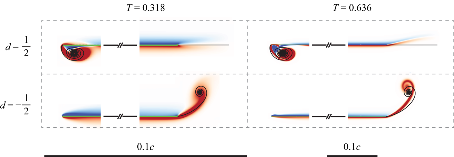
Using SVT, Hinton et al. (Reference Hinton, Leonard, Pullin and Sader2024) predicted that plate rotation about either its quarter-chord and three-quarter-chord positions, i.e.  $d = \pm 1/2$, can produce vortices of different types at the leading and trailing edges. Figure 12 shows a comparison of this inviscid prediction with the DNS.


In line with Hinton et al. (Reference Hinton, Leonard, Pullin and Sader2024), plate rotation about the three-quarter-chord position,  $d=1/2$, produces type III and II vortices at the leading and trailing edges, respectively. Moreover, the level of agreement between SVT and the DNS as time evolves, is commensurate with the discussion in the previous sections. Note that the theory in § 3 for
 $T_{max}$ does not apply to cases where
 $d=\pm 1/2$, as discussed.
Plate rotation about the quarter-chord position,  $d=-1/2$, completely suppresses the leading-edge vortex at the smaller time of
 $T = 0.318$ in figure 12. This again agrees with the prediction of SVT. Doubling the measurement time to
 $T = 0.636$ produces a small separation bubble at the leading edge. This corresponds to an instantaneous angle of attack of
 $\alpha \approx 3.5^\circ$, which further highlights the robustness of SVT and the utility of calculating the starting vortices. The trailing edge generates a type-III vortex, again in agreement with SVT; the agreement is superior for the smaller time, as expected. Note that the SVT trailing-edge vortices for
 $d = -1/2$ (bottom row of figure 12) are identical to those reported in the bottom row of figure 11; the corresponding DNS trailing-edge vortices are also similar in form. This validation of SVT reinforces its implications to the aerofoil design of low-speed aircraft, such as micro air vehicles (MAVs) and unmanned air vehicles (UAVs), which were discussed in Hinton et al. (Reference Hinton, Leonard, Pullin and Sader2024). Dynamic suppression of the leading-edge vortex can also affect thrust generation in flapping wings (Alben Reference Alben2010; Fang et al. Reference Fang, Ho, Ristroph and Shelley2017; Heydari & Kanso Reference Heydari and Kanso2021).
The corresponding total circulations in the trailing-edge vortices are reported in table 7. Agreement is again observed, with a larger discrepancy in the bottom left-hand entry of table 7. This again coincides with significant diffusion in the DNS trailing-edge vortex in the bottom left-hand entry of figure 12; see previous paragraph and the corresponding discussion at end of § 4.3.2 for an explanation of this discrepancy.


5. Joukowski aerofoil
We conclude our study by considering the Joukowski aerofoil which was studied in § 3.5 of Hinton et al. (Reference Hinton, Leonard, Pullin and Sader2024). The purpose is to assess the utility of SVT to an aerofoil of more complex shape. Two symmetric Joukowski aerofoils of different thickness are considered. The first is relatively thin with a Joukowski parameter of  $R = 1.1$, and is streamlined. The second is deliberately chosen to be bluff in its cross-section, with
 $R = 1.5$. Illustrations of these two aerofoils are given in figure 13.
The two symmetric Joukowski aerofoils considered in this study. Each has a sharp and straight trailing edge, which is evident by their upper and lower surfaces being tangent at the trailing edge. The Joukowski parameter,  $R$, is defined in (3.29) of Hinton et al. (Reference Hinton, Leonard, Pullin and Sader2024) and specifies the aerofoil thickness.

5.1. Starting-vortex inviscid theory
In line with § 3.5 of Hinton et al. (Reference Hinton, Leonard, Pullin and Sader2024), the aerofoil does not rotate but instead translates in two orthogonal directions with independent power laws in time. Specifically, each aerofoil moves with the following velocity components:
 \begin{equation} U(T)=U_0 {\mathcal{V}} T^{m}, \quad V(T) = U_0 {\mathcal{W}} T^{n}, \end{equation}
where  $U$ and
 $V$ are the velocity components parallel and perpendicular to the aerofoil's symmetric axis, respectively,
 $U_0$ is the dimensional velocity scale,
 ${\mathcal {V}}$ and
 ${\mathcal {W}}$ are dimensionless positive constants that control the relative magnitudes of the velocity components, and the translational power laws are
 $m,n\ge 0$.
We focus on the case of  $m=0$ and
 $n=2$ reported in § 3.5.1 of Hinton et al. (Reference Hinton, Leonard, Pullin and Sader2024). The SVT predicts that type-II vortices form at the trailing edge. Analytical formulas for the spatial extent of the trailing-edge vortex, the velocity jump across the trailing-edge vortex and its total circulation are given by
 $$\begin{gather} \frac{\gamma}{U_0} = \frac{8 \sqrt{2}}{3} \left(1 - \frac{x}{x_{max}} \right)^{{3}/{2}} \sqrt{\frac{{R}}{\mathcal{V}}} {\mathcal{W}} T^{3/2} , \quad 0 \le x \le x_{max}, \end{gather}$$
 $$\begin{gather}\frac{\varGamma_0}{U_0 a} = \frac{16 \sqrt{2}}{15} \sqrt{\frac{{\mathcal{V}}}{R}} {\mathcal{W}} \, T^{5/2}, \end{gather}$$
where the (dimensional) spatial extent of the wake is
 \begin{equation} x_{max} = \frac{{\mathcal{V}} T}{R} a, \end{equation}
and  $a$ is the half-chord of a Joukowski aerofoil with
 $R=1$;
 $x=0$ corresponds to the trailing edge of the Joukowski aerofoil (this differs from the origin of the flat plate above). Note that the chord length of the symmetric Joukowski aerofoil defined in (3.29) of Hinton et al. (Reference Hinton, Leonard, Pullin and Sader2024) is
 \begin{equation} c = \frac{2 R^2}{2R-1} a. \end{equation}
The dimensionless time,  $T$, is as defined in (1.2).
5.2. Direct numerical simulations
Figure 14 shows a comparison of the trailing-edge vortex calculated using SVT with the DNS; simulation parameters are reported in the caption of table 1. Agreement in the spatial extent of this vortex is observed especially for  $R = 1.1$. Some discrepancy emerges when the aerofoil's finite thickness (upstream from its trailing edge) becomes visible in the plots. In these cases, the wake's spatial extent exceeds that of the straight trailing edge and the vortex cannot be considered close to a ‘sharp and straight edge’ (see definition in § 1). This is a fundamental constraint of SVT and is consistent with the discrepancies observed in the second row of figure 14. Increasing the Reynolds above
 $Re =8000$ results in separation upstream of the trailing edge for
 $R=1.5$ (near the maximum width of the aerofoil), which complicates further numerical investigation.
Joukowski aerofoils. Type-II vortex:  $m=0$,
 $n=2$,
 ${\mathcal {V}}=1$,
 ${\mathcal {W}}=0.25$, for
 $Re =8000$; here
 $c$ is the chord of the aerofoil. Leading (left) and trailing (right) edges of the aerofoils are shown. Description as for figure 4.

Table 8 reports the total circulation in the trailing-edge wake, computed by SVT and DNS. The level of agreement is similar to that in table 4 for type-II vortices generated by a flat plate (for a much higher Reynolds number,  $Re = 32\,000$). Some discrepancy exists for
 $R=1.1$ with SVT overestimating the total wake circulation, especially for the smallest time. This appears to correlate with a wide and short wake, for which a vortex-sheet description may exhibit some error. The wake's aspect ratio (width over length) decreases with increasing time, which is seen to align with improved agreement between SVT and the DNS. Results for
 $R = 1.5$ in table 8 display enhanced agreement relative to
 $R=1.1$, with a similar trend for increasing time, despite the elongated wake of the DNS relative to SVT; see second row of figure 14. This is consistent with the vorticity generating mechanism (the aerofoil's no-slip condition) being decoupled from downstream effects where the flow accelerates (not included in SVT). These collective results for the total wake circulation align with those for the velocity jump distribution across the wake in figure 15. Agreement between SVT and DNS again improves slightly with increasing time (data not shown).
Joukowski aerofoil. Total dimensionless circulation,  $\bar \varGamma _0 \equiv \varGamma _0 /(U_0 a)$, in the trailing-edge vortex for the respective plots reported in figure 14; where
 $a$ is the half-chord of a Joukowski aerofoil for
 $R=1$. The entry positions in this table (and corresponding times,
 $T$) coincide with figure 14. Description as per table 2.

Joukowski aerofoil. Type-II vortex:  $m=0$,
 $n=2$, for
 $Re =8000$. Dimensionless velocity jump,
 $\gamma /U_0$, across the trailing-edge vortex. The DNS is evaluated by numerically integrating the vorticity distribution across the wake. The SVT for
 $\gamma /U_0$ is (5.2a). (a) Thinner aerofoil,
 $R=1.1$. (b) Thicker aerofoil,
 $R = 1.5$, where DNS data are shown to the spatial extent predicted by SVT; DNS data extend slightly further downstream. These plots correspond to trailing-edge wakes shown in the central column of figure 14.

6. Conclusions
Starting vortex inviscid theory predicts that three distinct types of starting vortex sheets – types I, II and III – can be generated by an arbitrary body with sharp and straight edges that suddenly moves. This study investigated the existence of these vortices in a viscous fluid for a flat plate and two symmetric Joukowski aerofoils.
The motion of a translating and rotating flat plate is characterised by two respective power laws in time,  $m$ and
 $p$, which select the vortex type. An abrupt transition between the starting-vortex types is predicted to occur in the
 $(m,p)$-phase plane; see figure 1. Type-I vortex sheets had been previously reported, while PS21 introduced types II and III to the literature and were yet to be observed in a (real) viscous fluid. Hinton et al. (Reference Hinton, Leonard, Pullin and Sader2024) extended these findings using inviscid theory to an arbitrary body with sharp and straight edges.
In this study, we reported a detailed assessment of these inviscid predictions using high-fidelity DNS of the Navier–Stokes equations. We also used SVT to calculate the time interval over which each starting-vortex type exists. It was found that for finite-time observations of a flat plate, there is a smooth (rather than abrupt) transition between the vortex types, as  $m$ and
 $p$ are varied. This is because the time interval over which type I and II vortices exist becomes vanishingly small as the critical
 $(m,p)$-phase plane line for type-III vortices is approached. We compared SVT with the DNS for values of
 $m$ and
 $p$ that span all vortex types. Agreement was observed when SVT was predicted to be valid. This included the velocity jump across a type-II vortex sheet and the total circulation in the wake of all vortex types. Moreover, different vortex types at the leading and trailing edges of a flat plate were observed in the DNS, for plate rotation about its quarter-chord and three-quarter-chord positions. Dynamic suppression of the leading-edge vortex for plate rotation about its quarter-chord position was confirmed. This position coincides with the aerodynamic centre of the aerofoil and is relevant to the aerofoil design of low-speed aircraft, such as MAVs and UAVs.
The predictions of SVT for two symmetric Joukowski aerofoils that translate in two orthogonal directions were also compared with DNS. Agreement was again observed for type-II vortices when their spatial extent does not exceed that of its sharp and straight edge – an overarching assumption of SVT. When this does occur, SVT was found to (i) underestimate the spatial extent of the wake, due to an accelerating flow downstream of the trailing edge, but (ii) accurately predict both the velocity jump across the wake and its total circulation. These comparisons highlight the utility of SVT for bodies of arbitrary shape.
This study confirms the existence of type II and III vortices in a viscous fluid, and validates the accuracy of SVT. We emphasise that SVT is predictive with no adjustable parameters. The inviscid theory reported by PS21, and its generalisation by Hinton et al. (Reference Hinton, Leonard, Pullin and Sader2024) for an arbitrary body – collectively referred to as the SVT – can therefore be used with confidence to calculate starting vortices in a viscous fluid.
Declaration of interests
The authors report no conflict of interest.
Appendix A. Additional time constraint for the existence of type I and II vortices generated by a flat plate
In this appendix, we derive the maximal time for type I and II vortices of a flat plate to exist, which supplements the time constraint in (3.5).
For type-I vortices, the second term on the right-hand side of (3.2) must dominate the first i.e.
 \begin{equation} {\rm i} \hat\beta \, T^{p-{q}/{2}} \frac{1 + M(Z) }{(2 Z)^{{1}/{2}}} \gg T^m, \end{equation}
where  $q = 2(\,p+1)/3$, as per table 1 of PS21. Balancing the left and right-hand sides of (3.2), gives
 $Z = O(\hat \beta ^{{2}/{3}})$, and the inequality in (A1) becomes
 \begin{equation} T^\epsilon \ll \hat\beta^{{2}/{3}}, \end{equation}
where
 \begin{equation} \epsilon \equiv m - \frac{2p-1}{3}, \end{equation}
which is strictly positive for a type-I vortex, i.e.  $\epsilon > 0$; see (1.6) and figure 1.
Type-II vortices occur in the opposite regime, i.e.
 \begin{equation} {\rm i} \hat\beta \, T^{p-{q}/{2}} \frac{1 + M(Z)}{(2 Z)^{{1}/{2}}} \ll T^m, \end{equation}
where  $q=1+m$. Balancing the left- and right-hand sides of (3.2) shows that
 $Z = O(1)$, from which (A4) becomes
 \begin{equation} T^{-({3}/{2}) \epsilon} \ll \hat\beta^{-1}, \end{equation}
where  $\epsilon < 0$ for type-II vortices.
Combining (A2) and (A5) produces
 \begin{equation} T^{| \epsilon |} \ll \hat\beta^{(2/3) \operatorname{sgn} (\epsilon)}, \end{equation}
where  $\epsilon \neq 0$; note that
 $\epsilon = 0$ corresponds to a type-III vortex sheet, which is not considered in this appendix. The time constraint in (A6) is in addition to (3.4), and the overarching spatial constraint that the vortex remains close to the trailing edge.
Choosing the same multiplicative factor as (3.5) for the inequality in (A6) to hold, i.e.  $0< \delta \ll 1$, gives the additional maximal time for existence of type I and II vortices
 \begin{equation} T_{max}^{(2)} \approx ( \hat\beta^{(2/3) \operatorname{sgn} (\epsilon)} \delta)^{1/| \epsilon |} , \end{equation}
where it is understood that  $\hat \beta$ is finite and the parenthesised term is less than unity. This shows that type I and II vortices, corresponding to
 $\epsilon > 0$ and
 $\epsilon < 0$, respectively, are more easily observed for large and small,
 $\hat \beta$, respectively. In § 3, we combine (A7) with (3.5) to give the overall maximal time for existence of any starting vortex.