





1. Introduction
Proper orthogonal decomposition (POD) is a widely used technique for extracting coherent structures from complex flow data. Originally introduced in fluid mechanics by Lumley (Reference Lumley1967), it decomposes a flow field into a set of orthogonal modes that capture most of the kinetic energy. In this framework, a fluctuating velocity field is expressed as a sum of spatial, orthogonal modes, each modulated by time-dependent coefficients, whose order is determined by their energy content (Weiss Reference Weiss2019). In its discrete form, POD is equivalent to principal component analysis (PCA), which consists in solving an eigenvalue problem for the data covariance matrix (Karhunen Reference Karhunen1947).
POD has been primarily developed and applied within an Eulerian framework. In this setting, the method is applied to a set of flow realizations, which correspond to instantaneous snapshots of the velocity field measured at fixed spatial locations. Each realization is represented by the spatial distribution of the velocity field, including all components, arranged into a single state vector. The decomposition is obtained by solving the eigenvalue problem associated with the data covariance operator. The resulting eigenvectors define an orthogonal set of spatial modes, while the corresponding eigenvalues quantify their kinetic energy. Two equivalent formulations of the Eulerian POD are commonly used. In the first – the snapshot method (Sirovich Reference Sirovich1987) – the covariance matrix is constructed from correlations between different realizations. In the second case, the covariance is constructed in physical space, thereby correlating spatial degrees of freedom across the dataset.
Despite POD’s widespread use in Eulerian problems in fluid mechanics, applications in Lagrangian settings – where fluid properties are prescribed along fluid parcel positions (Monin & Yaglom Reference Monin and Yaglom2013) – remain limited. Schiødt et al. (Reference Schiødt, Hodžić, Evrard, Hausmann, Van Wachem and Velte2022) developed a particle-POD method for inertial particles in decaying turbulence. Hassanian (Reference Hassanian2025) attempted to compare the distribution of POD mode energy from a Lagrangian experiment with Kolmogorov spectra, although how these are related is not yet clear. In the context of Lagrangian dynamics, Shinde & Gaitonde (Reference Shinde and Gaitonde2021) developed a POD routine called Lagrangian modal analysis that decomposes Lagrangian fields (the flow map) to identify coherent structures using space as a variable. The authors demonstrated that Lagrangian modal analysis can identify Lagrangian coherent structures in a manner similar to finite-time Lyapunov exponent analysis. In other contexts, PCA has been applied to particle trajectories, particularly in soft matter. For example, Chen et al. (Reference Chen, Liégeois, de Bruyn and Soddu2015) employed PCA at the image level to characterize particle motion, rather than as a modal decomposition of individual trajectories.
Since the introduction of Lagrangian experimental and numerical techniques roughly 30 years ago (Yeung & Pope Reference Yeung and Pope1989; Maas et al. Reference Maas, Gruen and Papantoniou1993; Malik et al. Reference Malik, Dracos and Papantoniou1993), the Lagrangian viewpoint has revealed numerous important phenomena related to dispersion (Biferale et al. Reference Biferale, Boffetta, Celani, Devenish, Lanotte and Toschi2005; Shnapp & Liberzon Reference Shnapp and Liberzon2018; Tan & Ni Reference Tan and Ni2022; Shnapp et al. Reference Shnapp, Brizzolara, Neamtu-Halic, Gambino and Holzner2023), energy transfer (Meneveau & Lund Reference Meneveau and Lund1994; Pumir et al. Reference Pumir, Shraiman and Chertkov2001) and intermittency (Biferale et al. Reference Biferale, Bodenschatz, Cencini, Lanotte, Ouellette, Toschi and Xu2008; Benzi et al. Reference Benzi, Biferale, Fisher, Lamb and Toschi2010) in turbulence, as well as properties of inertial particles therein (Bec et al. Reference Bec, Biferale, Lanotte, Scagliarini and Toschi2010). Nevertheless, our understanding of how the nonlinear multiscale interactions inherent to turbulent flows lead to these phenomena remains in its infancy. This work is motivated by the notion that a Lagrangian modal decomposition could help in this respect.
In this paper, we introduce a method, Lagrangian POD (LPOD), to decompose Lagrangian trajectories from a turbulent flow into orthogonal modes. We demonstrate its applicability using trajectories from both a direct numerical simulation (DNS) of homogeneous and isotropic turbulence (HIT) and a three-dimensional particle tracking (3D-PTV) experiment of quasi-HIT in a von Kármán flow. With an appropriate data arrangement and normalization, relatively long trajectories can be reconstructed using a limited number of modes, which appear to have a similar functional form in both the DNS and the experimental data. We also show that the method faithfully captures the intermittency of Lagrangian acceleration, velocity differences and curvature. The method has the potential to advance modelling and data compression in the context of the Lagrangian description of turbulent flows.
2. Methods
2.1. The LPOD routine
We consider the Lagrangian trajectories of tracer particles of a homogeneous, isotropic and stationary turbulent flow, which are defined as the solutions of the following equation:
 \begin{equation} \frac {{\rm d}\boldsymbol {x}}{{\rm d}t}=\boldsymbol {v}(\boldsymbol {x}(t),t), \qquad \boldsymbol {x}(t_0)=\boldsymbol {x}_0, \end{equation}
where
 $\boldsymbol {x}_0$
and
 $t_0$
denote the initial position and initial time, respectively, and
 $\boldsymbol {v}$
is the Eulerian velocity field. The corresponding Lagrangian velocity is given by
 $\boldsymbol {u}(\boldsymbol {x}_0,t_0;\tau ) = \boldsymbol {v}(\boldsymbol {x}(t_0+\tau ),t_0+\tau )$
, where
 $\tau =t-t_0$
is the time lag along the trajectory. The assumptions of statistical homogeneity and stationarity imply that the statistics of the Lagrangian velocity do not depend on
 $\boldsymbol {x}_0$
or
 $t_0$
, so these dependencies are henceforth omitted. A discrete ensemble of
 $N_p$
trajectories is considered, each represented by the velocity signal,
 \begin{equation} \frac {{\rm d}\boldsymbol {x}^{(p)}}{{\rm d}t} = \boldsymbol {u}^{(p)}(\tau )\textrm {,} \qquad p=1,\ldots ,N_p \textrm {,} \qquad \tau \in [0,\tau _{\textit{max}}] \end{equation}
where
 $p$
labels the trajectories in the ensemble and
 $\tau _{\textit{max}}$
is the duration of all trajectories. For each trajectory
 $p$
and velocity component
 $i=1,2,3$
, we define the temporal mean and standard deviation:
 \begin{align} \mu _i^{(p)}=\frac {1}{\tau _{\textit{max}}}\int _0^{\tau _{\textit{max}}} u_i^{(p)}(\tau )\,{\rm d}\tau = \frac {x_i^{(p)}(\tau _{\textit{max}}) - x_i^{(p)}(0)}{\tau _{\textit{max}}}\textrm {,} \\[-12pt]\nonumber \end{align}
 \begin{align} \sigma _i^{(p)} = \left ( \frac {1}{\tau _{\textit{max}}}\int _0^{\tau _{\textit{max}}} \big (u_i^{(p)}(\tau )-\mu _i^{(p)}\big )^2 {\rm d}\tau \right )^{1/2}\textrm {.} \end{align}
The normalized velocity fluctuation is then defined as
 \begin{equation} \tilde {u}_i^{(p)}(\tau ) = \big (u_i^{(p)}(\tau )-\mu _i^{(p)}\big )/\sigma _i^{(p)}\textrm {.} \end{equation}
Notably, as
 $\mu _i^{(p)}$
is defined per particle, the normalized velocity fluctuations do not impose any net displacement across the time
 $\tau _{\textit{max}}$
.
The LPOD is defined as a Karhunen–Loève expansion of these normalized Lagrangian velocity fluctuations,
 \begin{equation} \tilde {u}_i^{(p)}(\tau ) = \sum _{k=1}^{\infty } a_{i,k}^{(p)}\,\phi _k(\tau ), \end{equation}
where
 $\phi _k(\tau )$
are temporal modes and
 $a_{i,k}^{(p)}$
are the corresponding modal coefficients. The modes satisfy the orthogonality condition, namely
 $\int _0^{\tau _{\textit{max}}} \phi _k(\tau )\,\phi _{\ell }(\tau )\,{\rm d}\tau = \delta _{k\ell }$
. A truncated reconstruction using the first
 $K$
modes is obtained as
 \begin{equation} u_{i}^{(p,K)}(\tau ) = \mu _i^{(p)} + \sigma _i^{(p)} \sum _{k=1}^{K} a_{i,k}^{(p)}\,\phi _k(\tau )\textrm {,} \end{equation}
and the corresponding trajectory obtained by the truncated reconstruction is then computed by time integration:
 \begin{equation} \boldsymbol {x}^{(p,K)}(\tau ) = \boldsymbol {x}^{(p)}(0) + \int _0^\tau \boldsymbol {u}^{(p,K)}(s)\,{\rm d}s. \end{equation}
In practice, the velocity is available at discrete times
 $\tau _n=n\Delta \tau$
, with
 $n=1,\ldots , N_t$
, where
 $\Delta \tau$
is the time step with which the trajectory is sampled, or, equivalently, the inverse of the sampling frequency. The expansion is therefore approximated by applying PCA to the matrix of sampled normalized signals
 $U_{(p,i),n}=\tilde {u}_i^{(p)}(\tau _n)$
whose rows correspond to stacked trajectory velocity components and whose columns correspond to time samples. The eigenvectors of the temporal covariance matrix provide the discrete approximation of the modes
 $\phi _k(\tau _n)$
, while the projections of the signals onto these modes give the coefficients
 $a_{i,k}^{(p)}$
. A GitHub repository with Python implementation of the LPOD algorithm is available at Shnapp & Brizzolara (Reference Shnapp and Brizzolara2026).
2.2. Datasets description
We employ data from both a DNS of HIT and a 3D-PTV experiment. The DNS trajectories are integrated in a
 $1024^3$
HIT flow,
 $\textit{Re}_{\lambda } = 433$
, from the Johns Hopkins Turbulence Database – a widely used open database for exploring turbulence dynamics (Li et al. Reference Li, Perlman, Wan, Yang, Meneveau, Burns, Chen, Szalay and Eyink2008). Trajectories are
 $688$
frames long and are integrated with a time step of
 $\Delta \tau = 0.045 \tau _{\eta }$
, where
 $\tau _{\eta }$
is the Kolmogorov time scale. The total length of the trajectories corresponds to
 $\tau _{\textit{max}} = 30.77 \tau _{\eta } = 0.68 T_I$
, where
 $T_I$
is the integral time scale of the flow. The numerical dataset contains
 $5120$
trajectories. Trajectory data were downloaded directly from the online database via a MATLAB interface. Detailed information about this open database is available from Li et al. (Reference Li, Perlman, Wan, Yang, Meneveau, Burns, Chen, Szalay and Eyink2008).
The experimental trajectories are obtained from a low-seeding 3D-PTV experiment conducted in a von Kármán turbulence tank, which produces approximately zero-mean HIT at
 $\textit{Re}_{\lambda } \approx 150$
. The set-up is made of a circular 0.2 m diameter Poly(methyl methacrylate) (PMMA) cylinder enclosed inside a square tank, both filled with filtered tap water. The flow is driven by two smooth disks rotating in opposite directions at 3 Hz. Trajectories of 50 μm polyamide tracers (PSP50, Dantec Dynamics) have been identified using the MyPTV open-source software (Shnapp Reference Shnapp2022). The trajectories obtained through 3D-PTV vary in length, with shorter trajectories more likely and longer ones rarer. Unless otherwise specified, we considered trajectory chunks of
 $200$
frames, which correspond to an ensemble of
 $2607$
trajectories. The trajectories are sampled with a time step of
 $\Delta \tau = 0.09 \tau _{\eta }$
. The total length of the trajectories corresponds to
 $\tau _{\textit{max}} = 18.95\, \tau _{\eta } = 1.34 \,T_I$
. Further details about the experimental dataset and the evaluation of the integral and Kolmogorov scales are available in Appendix A.
2.3. Statistical observables
We introduce a set of statistical observables to assess the performance of truncated LPOD trajectory reconstructions, including modal properties, single-particle Lagrangian statistics, and geometric characteristics of the trajectories.
For the modal representation, we compute the projection coefficients associated with each mode, along with the corresponding variance explained, which quantifies the energy content of each principal component. To characterize Lagrangian transport, we first consider two dispersion-related observables: the mean-squared particle displacement and the deviation from ballistic motion, respectively:
 \begin{align} \big\langle \delta \boldsymbol {x}^2 \big\rangle &= \big\langle [\boldsymbol {x}(\tau ) - \boldsymbol {x}_0 ]^2 \big\rangle,\end{align}
 \begin{align} \big\langle \delta _b \boldsymbol {x}^2 \big\rangle &= \big\langle [\boldsymbol {x}(\tau ) - (\boldsymbol {x}_0 + \boldsymbol {u}(0)\,\tau ) ]^2 \big\rangle.\end{align}
The mean-squared displacement exhibits ballistic scaling for
 $\tau \ll T_I$
, namely
 $\langle \delta \boldsymbol {x}^2 \rangle \sim u_{\textit{rms}}^2 \tau ^2$
(Taylor Reference Taylor1922). The deviation from ballistic motion isolates the contribution of velocity fluctuations (Shnapp Reference Shnapp2019) and is expected to scale as
 $\langle \delta _b \boldsymbol {x}^2 \rangle \sim \epsilon \tau ^3$
in the inertial range (Obukhov Reference Obukhov1959), similarly to the scaling of the mean square separation between particle pairs (Richardson Reference Richardson1926). More details about the derivation of this scaling can be found in Appendix B material and in Monin & Yaglom (Reference Monin and Yaglom2013), equation (24.13).
We further consider the Lagrangian velocity increments, namely
 \begin{equation} \delta \boldsymbol {u}(\tau ) = \boldsymbol {u}(\tau ) - \boldsymbol {u}(0) \end{equation}
and their longitudinal component, defined as
 \begin{equation} \delta u_{\parallel } = \frac {\delta \boldsymbol {u}(\tau ) \boldsymbol{\cdot }(\boldsymbol {x}(\tau ) - \boldsymbol {x}_0)}{|\boldsymbol {x}(\tau ) - \boldsymbol {x}_0|}\textrm {.} \end{equation}
The
 $p$
th-order absolute value and longitudinal structure functions are defined as
 \begin{equation} S_p = \langle {|\delta \boldsymbol {u} (\tau )| }^p\rangle \textrm {,} \end{equation}
 \begin{equation} S_p^{\parallel }(\tau ) = \langle {\delta u_{\parallel } (\tau ) }^p\rangle \textrm {.} \end{equation}
In the inertial range, the second-order structure functions (
 $p=2$
) are expected to scale linearly with time, namely
 $S_2^{\parallel } \sim \epsilon \tau$
(Monin & Yaglom Reference Monin and Yaglom2013).
To challenge the capability of LPOD in reconstructing higher-order statistics associated with intermittency, we consider the scaling of the fourth- and sixth-order structure functions versus the second-order one, as well as the logarithmic derivative of
 $S_4$
versus
 $S_2$
, namely
 \begin{equation} \xi _4(\tau ) = \frac {{\rm d}\,\log (S_4)}{{\rm d}\,\log (S_2)}\textrm {.} \end{equation}
This latter quantity is a proxy for intermittency and has been found to exhibit a universal functional form across several datasets and different Reynolds numbers (Arnéodo et al. Reference Arnéodo2008; Toschi & Bodenschatz Reference Toschi and Bodenschatz2009).
An additional strongly intermittent observable is the absolute value of the Lagrangian acceleration, namely the material derivative of the Lagrangian velocity:
 \begin{equation} a(\tau ) = |\boldsymbol {a}(\tau )| \textrm {,} \quad \boldsymbol {a}(\tau ) = \frac {{\rm d} \boldsymbol {u}(\tau )}{{\rm d} \tau }\textrm {.} \end{equation}
The probability distribution of
 $|\boldsymbol {a}|$
is heavy-tailed and, at sufficiently high Reynolds number, it is believed to possess a universal shape when normalized by the Kolmogorov scales (Toschi & Bodenschatz Reference Toschi and Bodenschatz2009).
Finally, we consider the curvature as a proxy of for the trajectories’ geometry:
 \begin{equation} \kappa = \frac {|\boldsymbol {u} \times \boldsymbol {a}|}{|\boldsymbol {u}|^3}\textrm {.} \end{equation}
At sufficiently high Reynolds number, the curvature distribution exhibits a power-law behaviour that scales linearly for small curvatures and as
 $\kappa ^{-2/5}$
for large curvatures (Braun et al. Reference Braun, De Lillo and Eckhardt2006; Xu et al. Reference Xu, Ouellette and Bodenschatz2007).
3. Results
3.1. LPOD modes and their energy
(a) First 10 LPOD modes: solid lines denote DNS data and dashed lines 3D-PTV data. (b) Example DNS trajectory reconstruction using an increasing number of modes (2, 4, 8 and 16); the dashed line shows the ballistic reconstruction from the mean velocity, and the black line the original trajectory. (c) Energy distribution (explained variance) normalized such that
 $\sum _{k=1}^{N_t} E_k = 100$
; solid and dashed lines correspond to DNS and 3D-PTV data, respectively. The inset shows the same data in square-log coordinates to highlight the subexponential decay.

We start by presenting the results of LPOD applied to both the numerical and experimental datasets described in § 2. Figure 1(a) shows the first 10 modes of the expansion, where the time is normalized with the trajectory duration and the intensity with the first value (the value at
 $\tau = 0$
). In both the experiment and the simulation, progressively higher-order modes capture higher-frequency velocity fluctuations. By comparing the leading modes obtained from the experiments (dashed lines) and the simulation (solid line), we observe that the mode shapes are similar in both cases. Figure 1(b) shows an example of truncated reconstruction for a topologically complex trajectory from the DNS data. Although truncated at the 16th mode, the reconstruction of this example trajectory qualitatively matches the ground truth. The similarity between the modes from the two datasets is an important feature of LPOD, as it has significant potential for data reconstruction, compression and modelling. This result is, in fact, expected, as a well-known feature of the orthogonal decomposition is that statistically stationary signals decompose into the harmonic basis of a discrete Fourier transform (George Reference George1988). Since the flow considered here is stationary, homogeneous and isotropic (nearly so in the experiment), the trajectories are expected to follow stationary statistics, which is encapsulated in the modes we obtained. Deviations from ideal HIT behaviour are evident in the differences between the two datasets, which become progressively more pronounced as
 $k$
increases. These discrepancies arise because the experimental flow is sampled with finite-size particles and the DNS dataset is not perfectly stationary, situations that cannot be represented by purely periodic modes (Hodžić et al. Reference Hodžić, Olesen and Velte2024). Notably, orthogonal decomposition strategies are also very relevant for inhomogeneous or non-stationary flows or those that are homogeneous in some ways but not others, as discussed by George (Reference George1988).
(a) Convergence profile of the first eight modes, namely the cosine between the
 $k$
th mode computed using the whole dataset (
 $\phi ^{(k)}$
) and the ones computed with a subsample of
 $S$
trajectories (
 $\phi ^{(k)}_S$
); each profile is computed by averaging the results of
 $100$
bootstrap resamples of the dataset. (b) Heatmap of the total energy captured by the first
 $k$
modes for different trajectory durations
 $\tau$
; the solid lines are isolines corresponding to
 $90$
%,
 $99$
%,
 $99.9$
% and
 $99.99$
% of the total energy. Both graphs are obtained using the DNS dataset.

Figure 1(c) shows the percentage of energy content associated with each mode (its eigenvalue) for the experiments and DNS data. As with PCA analyses, most of the energy in LPOD is concentrated in the first few modes, with the first 10 modes accounting for 99 % of the kinetic energy. As highlighted by the inset of figure 1(c), the mode energy decreases subexponentially, approximately as
 $e^{-(k/C)^{1/2}}$
, where
 $C$
is a constant, up to
 $k\approx 100$
. For
 $k$
larger than this, the deviation between the experimental and numerical cases becomes more significant. Several factors may lead to discrepancies between datasets for high-order modes. First, the two datasets are characterized by heavily different Reynolds numbers (
 $\textit{Re}_{\lambda }=433$
for the simulations and
 $\textit{Re}_{\lambda }\approx 150$
for the experiments). Second, the temporal sampling rates differ substantially: the simulation data are sampled at approximately 10 times the frequency of the experimental data when expressed in Kolmogorov time units. Third, the total trajectory length differs between the two datasets in both Kolmogorov time units and integral time units (see § 2.2). As a result, the experimental trajectories contain fewer samples (200) than the simulated ones (688), leading to a correspondingly smaller number of modes. Since the explained energy is expressed as a percentage of the total variance, this difference necessarily affects the distribution of energy among the highest-order modes.
As suggested by the energy distribution differences found between the two datasets, the performance of LPOD may depend on the trajectory duration. On the one hand, longer trajectories are expected to require a larger number of modes to be accurately represented; on the other hand, estimating higher-order modes is expected to require increasingly large ensembles of trajectories in the dataset. To quantify the effect of the dataset size on the representation of the modes, we report in figure 2(a) the convergence profiles of the first eight modes, quantified by the cosine similarity between the
 $k$
th eigenfunction computed using the full dataset and that obtained from a random subset of trajectories. As the sample size increases, this similarity approaches unity, indicating convergence of the estimated mode. As expected, higher-order modes (large
 $k$
) converge more slowly and therefore require more trajectories to be reliably identified. To quantify the effect of trajectory duration, we compute the cumulative explained energy captured by the first
 $k$
modes as a function of trajectory length. Figure 2(b) shows isolines of cumulated explained energy, demonstrating that progressively longer trajectories require an increasing number of modes to capture the same fraction of the total energy. For instance, five modes capture approximately
 $99\,\%$
of the energy for trajectories of duration
 $0.2,T_I$
, whereas trajectories of duration
 $0.6,T_I$
require approximately 10 modes to achieve the same level of cumulated energy.
3.2. Reconstructing Lagrangian statistics
We present the Lagrangian statistics defined in § 2.3 for both the original and reconstructed trajectories. Figure 3 shows Lagrangian single-particle dispersion statistics. Considering the mean-squared displacement, figure 3(a) shows that the truncated reconstruction done with 16 modes is indistinguishable from the original signal. This is expected, since the mean velocity for each trajectory is removed prior to the decomposition and reintroduced during reconstruction. As a result, the ballistic contribution to the displacement is preserved exactly, so that, in the ballistic regime, the mean-squared displacement is recovered, even in the absence of fluctuating modes. To better assess the limits of the truncated representation on the single-particle dispersion process, we consider the deviation from ballistic motion
 $\langle \delta _bx^2\rangle$
, shown in figure 3(b). This quantity is more sensitive to small-scale velocity fluctuations and is therefore more difficult to reconstruct, particularly at short time lags. Nevertheless, a relatively small number of modes (16) is sufficient to recover the correct behaviour for lags exceeding a few Kolmogorov time scales, when the data are expected to exhibit inertial-range scaling. To assess the impact of the number of modes on the reconstruction of
 $\langle \delta _bx^2\rangle$
, we evaluate the relative reconstruction error, defined as the ratio between the difference of the reconstructed and original signals and the original signal itself. This is shown in the inset of figure 3(b) as a function of both the time lag and the number of retained modes, demonstrating that adding modes reduces the relative error at progressively shorter time lags (smaller scales).
(a) Mean-square displacement obtained by the DNS dataset; the inset shows the data normalized by the ballistic scaling. (b) Mean square of the deviation-from-ballistic motion; the inset shows the relative reconstruction error
 $\delta _b^{(k)}x_{ {\,err.\,\%}} = 100 \times |\langle \delta _b^{(k)} x ^2 \rangle - \langle \delta _b x ^2 \rangle | / \langle \delta _b x ^2 \rangle$
computed with progressively more modes. In both panels, orange and blue markers denote the original data and the 16-mode truncation, respectively.

The second-order longitudinal structure function is accurately reconstructed for lags larger than a few Kolmogorov time scales using 16 modes only (figure 4 a). The inset shows the relative reconstruction error, demonstrating that reconstruction improves at progressively shorter lags as more modes are added. Figure 4(b) shows the probability density functions (PDFs) of the longitudinal normalized velocity increments for increasing time lags. As the lag increases, the distributions approach Gaussian behaviour. Reconstructions based on a limited number of modes (16) underestimate the tails at short time lags when the distribution is strongly non-Gaussian, whereas they are accurate for longer time lags as Gaussianity is approached.
(a) Second-order longitudinal structure function computed from the DNS dataset (orange circles denote the original data, whereas blue diamonds are obtained from the first 16 modes); the inset shows the relative reconstruction error
 ${S_2^{\parallel }}^{(k)}_{ {err.\,\%}} = 100 \times |{S_2^{\parallel }}^{(k)} - {S_2^{\parallel }}| / {S_2^{\parallel }}$
computed with progressively more modes. (b) The PDF of the velocity increments from the DNS dataset. The time lag varies from
 $0.1$
to
 $30\,\tau _{\eta }$
. The reconstructed data (blue solid lines) are obtained using the first 16 modes; the orange circles are the original data. The data are normalized with the structure function computed from the original data for both cases.

(a) Fourth- (
 $S_4$
, orange circles) and sixth-order (
 $S_6$
, orange triangles) structure functions plotted against the second-order one (
 $S_2$
); continuous and dashed lines are the reconstructed signals of
 $S_4$
and
 $S_6$
, respectively; the colour intensifies with the number of modes, from
 $4$
(lighter blue) to
 $32$
(darker blue);
 $S_6$
is multiplied by a factor
 $1000$
for clarity. (b) Logarithmic derivative of
 $S_4$
versus
 $S_2$
, as defined in (2.14), versus time lag. The orange circles denote the original signal, while the blue lines correspond to reconstructions using 4, 8, 16 and 32 modes (colours from light to dark blue). The curves are obtained from experimental data, using trajectories of duration
 $\sim 10\, \tau _{\eta }$
(100 frames, half the duration of the long trajectories used elsewhere) to improve statistics.

Figure 5. Long description
Panel A: A scatter plot shows the fourth- and sixth-order structure functions plotted against the second-order structure function. Orange circles represent the fourth-order structure function, and orange triangles represent the sixth-order structure function. Continuous and dashed lines are the reconstructed signals of the fourth- and sixth-order structure functions, respectively. The color intensifies with the number of modes, ranging from lighter blue to darker blue. The sixth-order structure function is multiplied by a factor for clarity. Panel B: A line graph displays the logarithmic derivative of a variable versus time lag. Orange circles denote the original signal, while blue lines correspond to reconstructions using 4, 8, 16, and 32 modes, with colors ranging from light to dark blue. The curves are derived from experimental data using trajectories of a specific duration to improve statistics.
To test the LPOD capabilities with regard to intermittency, we compute the fourth- and sixth-order structure functions. To this purpose, we employed the experimental dataset, extending it by using trajectories as short as
 $10\,\tau _{\eta }$
(100 frames). In this form, the experimental dataset contains approximately
 $32\,500$
trajectories (see further details in Appendix A), enough to compute the scalings of higher-order structure functions. Figure 5(a) shows that the scaling of
 $S_4$
and
 $S_6$
versus
 $S_2$
can be correctly reconstructed by using
 $32$
modes. Similarly, figure 5(b) demonstrates that 32 modes are sufficient to reconstruct the signal of the logarithmic derivative of
 $S_4$
with respect to
 $S_2$
(equation (2.14)), although the original signal is noisy due to the still moderate number of trajectories in the dataset. As demonstrated in § 3.1, the shorter trajectories employed in this analysis are easier to reconstruct, while longer trajectories are expected to require a larger number of modes. Furthermore, the present trajectory duration, approximately
 $10\tau _\eta$
, is too short to robustly identify an inertial-range scaling regime, since contamination from dissipative effects – in fact, linked to intermittency – remain significant at these time lags (Arnéodo et al. Reference Arnéodo2008).
(a) The PDF of the trajectory acceleration computed from the DNS data. The orange line denotes the original signal, while the blue lines correspond to reconstructions using 4, 8, 16 and 32 modes. (b) Kurtosis
 $\mathcal{K}$
of the reconstructed acceleration normalized by the original signal’s Kurtosis; dashed and solid lines indicate experimental and DNS data, respectively; the inset shows the same curves with the mode number multiplied by
 $\Delta \tau /\tau _{\eta }$
.

Figure 6(a) shows the probability distribution of the trajectory acceleration for the DNS data. The acceleration distribution, as the longitudinal structure function at small time lags, requires high-order modes to be captured accurately. Indeed, the variance of the acceleration is proportional to the longitudinal structure function for vanishing time lags (see (24.12) in Monin & Yaglom Reference Monin and Yaglom2013), which has been shown to require a relatively high number of modes to be accurately reconstructed (see the inset of figure 4
a). However, even by using 32 modes, the tail of the acceleration distribution is hard to correctly capture: this discrepancy is due to the inherent difficulties of compressing the strongly intermittent signal of the Lagrangian acceleration for these relatively long numerical trajectories. To better highlight this aspect, figure 6(b) shows the ratio of the Kurtosis of the reconstructed acceleration to that of the original data: up to
 $80$
modes are required to fully recover the extreme acceleration events in the DNS data (continuous line), whereas a smaller number (
 $\approx 40$
) suffices for the experimental data (dashed line). As such, approximately 0.1 % and 1.0 % of the trajectories’ turbulent kinetic energy is needed to resolve acceleration intermittency in the numerical and experimental data, respectively. Here, the difference between the experiments and the DNS data is likely due to difference in Reynolds number (
 $\textit{Re}_{\lambda } \approx 150$
in the experiments versus
 $430$
in the DNS), trajectory length (
 $\tau _{\textit{max}} = 19.76 \tau _{\eta }$
in the experiments versus
 $30.85 \tau _{\eta }$
in the DNS), and sampling frequency (
 $10/\tau _{\eta }$
in the experiments versus
 $25/\tau _{\eta }$
in the DNS). We observe that, by normalizing the mode number
 $k$
by the normalized sampling frequency
 $\tau _{\eta }/\Delta \tau$
, the DNS and experimental Kurtosis collapse on the same master curve (see the inset of figure 6
b).
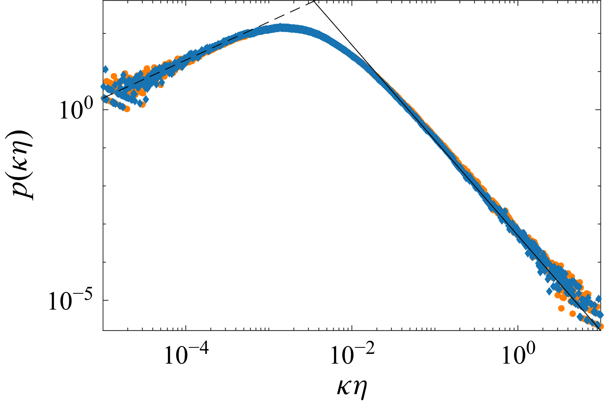
Figure 7 shows the probability distribution of the trajectory curvature for the DNS data. From this perspective, the reconstructed and original signals appear indistinguishable, indicating that the first 16 modes accurately capture the trajectories’ geometry. This result is surprising, as the curvature contains both the velocity and acceleration in its definition, the latter being difficult to reconstruct with few modes, especially concerning the tails of the distribution. A possible explanation for this observation is that curvature is more correlated with low velocity than with high acceleration (Xu et al. Reference Xu, Ouellette and Bodenschatz2007), making it more sensitive to large scale flow features than to intermittent acceleration events; then, as our method normalizes the velocity fluctuations it make it more robust for faithfully reconstructing this geometrical aspect.
The PDF of the trajectory curvature (DNS dataset). Orange and blue markers are the original and reconstructed (16 modes) data, respectively, while the dashed and solid lines indicate the dimensional scalings
 $\kappa ^{1}$
and
 $\kappa ^{-5/2}$
for small and large curvatures, respectively. Data are logarithmically binned.

4. Discussion and outlook
In this paper, we introduced a new method for analysing Lagrangian trajectories using PCA, which can be viewed as a Lagrangian analogue of standard POD. To the best of our knowledge, the only attempt to perform POD on Lagrangian trajectories was by Schiødt et al. (Reference Schiødt, Hodžić, Evrard, Hausmann, Van Wachem and Velte2022), but with a different approach. In their work, the authors normalized the data with ensemble averages, which are not suited for isolating the fluctuating velocities of each trajectory and do not preserve the total displacement over the full trajectory length. In contrast, our normalization ensures that the truncated reconstructions always begin and end at the same locations as the original trajectories. This is well illustrated by figure 1(b), which shows that the total drift along each trajectory is preserved by construction, regardless of the number of modes used. Encoding this normalization in the data also renders the single particle dispersion accurately reconstructible with an extremely low number of modes, as shown in figure 3(a), because, for lags shorter than the integral time scale, the process is ballistic (Taylor Reference Taylor1922). However, while this approach preserves the initial and final positions by construction, it does so at the cost of storing the temporal mean and standard deviation for each trajectory separately.
By analysing the statistics of truncated reconstructions, we show that LPOD’s performance depends on the time lag considered, on the trajectories’ length, and on the Reynolds number. For a fixed Reynolds number and trajectory duration, quantities defined at intermediate and long lags are accurately reconstructed with a small number of modes, whereas observables based on short-time lags, such as acceleration and short-time velocity increments, require a significantly larger number of modes to converge. This reflects the strong intermittency (see, e.g. La Porta et al. (Reference La Porta, Voth, Crawford, Alexander and Bodenschatz2001) and Mordant et al. (Reference Mordant, Metz, Michel and Pinton2001)) associated with these quantities, which requires higher frequencies and thus higher-order modes to be accurately captured. In general, higher-order statistical observables, in particular the fourth- and sixth-order structure functions, require more modes to be accurately reconstructed, allegedly a consequence of the intrinsic
 $L_2$
variance optimality of LPOD.
By plotting the normalized acceleration Kurtosis as a function of the number of retained modes, we observe that scaling the mode number with the sampling frequency normalized by the Kolmogorov time collapses the data on the same master curve. This suggests that, if the data were sampled at the same normalized frequency, the number of modes needed to reconstruct the acceleration signals would have been Reynolds number and trajectory-length-independent. In other words, the degree of complexity needed for reconstructing acceleration statistics seems to be proportional to the length of the trajectories in terms of Kolmogorov times, regardless of whether this is set by the Reynolds number of the flow or by their length.
Finally, LPOD may serve as a starting point for modelling, particularly for generating synthetic trajectories. This task has been traditionally addressed with stochastic models (see, e.g. Thomson (Reference Thomson1987), Pope & Chen (Reference Pope and Chen1990), Sawford (Reference Sawford1991), Wilson et al. (Reference Wilson, Yee, Ek and d’Amours2009) and Shnapp et al. (Reference Shnapp, Bohbot-Raviv, Liberzon and Fattal2020)) and recently using deep-learning techniques, e.g. diffusion networks (see, e.g. Li et al. Reference Li, Biferale, Bonaccorso, Scarpolini and Buzzicotti2024a , Reference Li, Tommasi, Buzzicotti, Bonaccorso and Biferaleb , Reference Li, Biferale, Bonaccorso, Buzzicotti and Centurioni2025) or data-informed stochastic models based on neural networks (de Wit et al. Reference de Wit, Gabbana, Woodward, Lin, Toschi and Livescu2026). Applying LPOD to two different dataset of isotropic turbulence generated with different techniques and forcing conditions, we showed that the shape of the modes appears to only weakly depend on the turbulence under consideration, and may thus be universal – albeit only two cases (one DNS and one experiment) are reported here; this suggests that learning the joint probability distribution of the modes coefficient and stochastic sampling from it may be sufficient to construct synthetic Lagrangian turbulence. However, further investigation and testing of non-homogeneous, non-stationary and non-isotropic turbulent flows are needed to assess the mode shapes in different contexts.
Declaration of interests
The authors report no conflict of interest.
Appendix A. Characterization of the experimental dataset
In the experiment, the flow is sustained in a von Kármán turbulence generator using filtered tap water inside a cylindrical volume, 18 cm in height and 18 cm in diameter. The flow is generated by two counter-rotating smooth discs, driven via two step motors to rotate at 150 revolutions per minute. Four synchronized cameras are used to image tracer particles in the flow (50 μm, PSP50 from Dantec Dynamic), viewing approximately 1500 particles per frame, located within a rectangular volume measuring 100
 $\times$
100
 $\times$
50 mm at the centre of the cylinder – see figure 8(c) for a snapshot of the three-dimensional trajectories. The velocity in the region of measurement is, to a good approximation, zero-mean with Gaussian fluctuations whose root mean square is approximately
 $u_{\textit{rms}} \approx 2.87 \times 10^{-2}\rm\,m\,s^{-1}$
with
 $10\,\%$
difference between the vertical and horizontal directions. In agreement with previous studies (see, e.g. Chevillard et al. (Reference Chevillard, Roux, Lévêque, Mordant, Pinton and Arnéodo2003) and Shnapp (Reference Shnapp2019)), the PDF of Lagrangian velocity differences relaxes from a heavy-tailed distribution to a Gaussian distribution across the inertial range (figure 8
b), demarcating small-scale intermittency. The energy dissipation rate can be computed following different approaches. Considering the second-order Lagrangian structure function with a standard value of the constant
 $C_0 = 3$
, we obtain
 $\epsilon \approx 8.2 \times 10^{-4}\rm \,m^2\,s^{-3}$
, see figure 8(a). Considering the equilibrium formulation (Frisch & Donnelly Reference Frisch and Donnelly1996), we obtain
 $\epsilon = C_\epsilon \, {u_{\textit{rms}}}^3/L_I = 6.4 \times 10^{-4}\rm\,m^2\,s^{-3}$
using
 $C_\epsilon = 0.5$
, where the integral length scale obtained by fitting the Eulerian correlation function is
 $L_I = 18.6\rm\,mm$
(see figure 9
a). Considering the third-order Eulerian longitudinal structure function and the
 $4/5$
law (Frisch & Donnelly Reference Frisch and Donnelly1996), we obtain
 $\epsilon = 4.7 \times 10^{-4}\rm \,m^2\,s^{-3}$
(fit shown in figure 9
b).
(a) Lagrangian second-order structure functions for the
 $x$
(top) and
 $y$
(bottom) velocity components, normalized with Kolmogorov scaling with
 $C_0=3$
; the peaks allow to estimate the dissipation rate as
 $\epsilon \approx 820$
 $\mathrm{mm^2}\,\mathrm{s^{-3}}$
. (b) The PDFs of Lagrangian velocity increments, normalized by their standard deviation and vertically translated for
 $\tau /\tau _\eta \approx 0.6$
, 3, 6 and 12, demonstrating the change of the PDF with time lag, commonly referred to as small-scale intermittency. (c) A Rendering of trajectories from the experiment, where the shade indicates the velocity magnitude.

Throughout the manuscript we consider the energy dissipation rate as obtained from the third-order structure function, namely
 $\epsilon = 4.7 \times 10^{-4}\rm \,m^2\,s^{-3}$
, which provides
 $\tau _{\eta } = 0.046\rm\,s$
,
 $\eta = 2.14 \times 10^{-4}\rm\,m$
and the Taylor microscale
 $\lambda = u_{\textit{rms}}\sqrt {{15 (\nu / \epsilon )}} = 5.1 \times 10^{-3} \rm \,m$
. We consider as integral time scale
 $T_I = L/u_{\textit{rms}} = 0.65\rm \, s$
. The corresponding Reynolds numbers are
 $\textit{Re}_\lambda \approx 140$
and
 $\textit{Re}_L \approx 530$
. These estimates are the one that allows the most direct comparison with the numerical dataset (see Li et al. Reference Li, Perlman, Wan, Yang, Meneveau, Burns, Chen, Szalay and Eyink2008).
(a) Eulerian velocity autocorrelation function. (b) Second- and third-order Eulerian longitudinal structure functions.

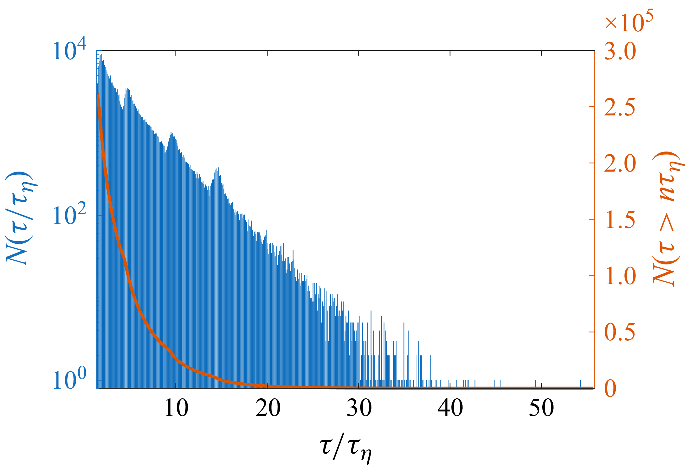
As discussed in § 3.2, the 3D-PTV approach yields a set of trajectories with varying lengths. Shorter trajectories are more common than longer trajectories. Figure 10 shows the histogram of the number of trajectories per duration, binned per frame, demonstrating that the most likely trajectories have a duration of
 $5-10\,\tau _{\eta }$
. As shown by the figure, longer trajectories are exponentially less frequent. The red line represents the number of trajectories longer than a given duration. Only
 $\approx 2500$
trajectories longer than
 $20\tau _{\eta }$
are available; while considering trajectories as short as
 $10\tau _{\eta }$
, the dataset can be extended to
 $32\,500$
trajectories.
Number of trajectories per trajectory duration. Blue is the number of trajectories of a given duration, while the red curve is the cumulative sum, namely the number of trajectories longer than
 $n$
times the Kolmogorov time scale.

Appendix B. Derivation of the scaling for the mean-square of the deviation-from-ballistic
We report the derivation of the mean-square of the deviation from ballistic motion presented by Obukhov (Reference Obukhov1959) and reported by Monin & Yaglom (Reference Monin and Yaglom2013), equation (24.13). We consider the deviation-from-ballistic vector
 $\delta _b \boldsymbol {x} = \boldsymbol {x}(\tau ) - \boldsymbol {x}(t) - \boldsymbol {u}(t)\,\tau$
and derive both sides respect to
 $\tau$
:
 \begin{equation} \frac {{\rm d}\,\delta _b \boldsymbol {x}}{{\rm d}\,\tau } = \boldsymbol {u}(t+\tau )-\boldsymbol {u}(t). \end{equation}
By multiplying both sides of (B1) by
 $\delta _b \boldsymbol {x}$
, we obtain
 \begin{equation} \delta _b \boldsymbol {x} \boldsymbol{\cdot }\frac {{\rm d}\,\delta _b \boldsymbol {x}}{{\rm d}\tau _2} = [\boldsymbol {u}(t+\tau _2)-\boldsymbol {u}(t)] \boldsymbol{\cdot }\int [\boldsymbol {u}(t+\tau _1) - \boldsymbol {u}(t)]\,{\rm d}\tau _1. \end{equation}
The left-hand side is equal to
 $({1}/{2})({{\rm d}\,\delta _b x^2}/{{\rm d}\,\tau _2})$
, so integrating the above with respect to
 $\tau _2$
:
 \begin{equation} \delta _b x^2 = 2\int [\boldsymbol {u}(t+\tau _2)-\boldsymbol {u}(t)]\,{\rm d}\tau _2 \boldsymbol{\cdot }\int [\boldsymbol {u}(t+\tau _1)-\boldsymbol {u}(t)]\,{\rm d}\tau _1. \end{equation}
Combining the integral and averaging gives
 \begin{equation} \big\langle \delta _b x^2 \big\rangle = 2\iint \langle [\boldsymbol {u}(t+\tau _1)-\boldsymbol {u}(t)]\boldsymbol{\cdot }[\boldsymbol {u}(t+\tau _2)-\boldsymbol {u}(t)]\rangle \, {\rm d}\tau _1\,{\rm d}\tau _2. \end{equation}
Expanding the terms in parentheses by computing the scalar product and using the isotropy of the velocity statistics yields
 \begin{equation} \big\langle \delta _b x^2 \big\rangle = 6 \iint [R(\tau _2-\tau _1) - R(\tau _2) - R(\tau _1) +R(0)] \,{\rm d}\tau _1 \, {\rm d}\tau _2 \end{equation}
where
 $R(\tau -t) = \langle u(t+\tau )u(t)\rangle$
is the two-times velocity correlation function. The velocity correlations can be written in terms of the structure function, since, by definition,
 $S_2 =2( R(t) - R(\tau -t))$
. This yields
 \begin{equation} \big\langle \delta _b x^2 \big\rangle = 3 \iint [ S_2(\tau _1) + S_2(\tau _2) - S_2(|\tau _2 - \tau _1|)] \,{\rm d}\tau _1 \, {\rm d}\tau _2\textrm {,} \end{equation}
where the absolute value
 $|\tau _2 - \tau _1|$
is due to the symmetry of the correlation function. Within the inertial range of turbulence, we can plug the Kolmogorov scaling ansatz
 $S_2 = C_0 \epsilon t$
where
 $C_0$
is the Lagrangian, single-component, Kolmogorov constant and get
 \begin{equation} \big\langle \delta _b x^2 \big\rangle = 3\,C_0 \epsilon \iint \left ( \tau _1 + \tau _2 - |\tau _2 -\tau _1| \right ) \,{\rm d}\tau _1 \, {\rm d}\tau _2 = 3\,C_0 \epsilon \iint \min (\tau _1,\tau _2) \,{\rm d}\tau _1 \, {\rm d}\tau _2\textrm {,} \end{equation}
which, computing the integral leads to
 \begin{equation} \big\langle \delta _b \boldsymbol {x}^2 \big\rangle = \frac {C_0}{2}\epsilon \tau ^3\textrm {,}\qquad \tau _{\eta } \ll \tau \ll T_I. \end{equation}
For short times (
 $\tau \ll \tau _\eta$
), we can approximate
 $\delta _b \boldsymbol {x}$
through a Taylor expansion as
 \begin{equation} \delta _b \boldsymbol {x} = \frac {1}{2} \langle {\boldsymbol {a}} ^2\rangle \tau ^2 + O (\tau ^3) \end{equation}
which, using the scaling
 $\langle {\boldsymbol {a}} ^2\rangle \sim \eta /\tau _{\eta }^2$
leads to a power four scaling:
 \begin{equation} \langle \delta _b \boldsymbol {x}^2 \rangle \sim \eta ^2 \left ( t/\tau _{\eta }\right )^4. \end{equation}

 ∑k=1NtEk=100

 k
 ϕ(k)
 S
 ϕS(k)
 100
 k
 τ
 90
 99
 99.9
 99.99

 δb(k)xerr.%=100×|⟨δb(k)x2⟩−⟨δbx2⟩|/⟨δbx2⟩

 S2∥err.%(k)=100×|S2∥(k)−S2∥|/S2∥
 0.1
 30τη

 S4
 S6
 S2
 S4
 S6
 4
 32
 S6
 1000
 S4
 S2
 ∼10τη

 K
 Δτ/τη
 κ1
 κ−5/2

 x
 y
 C0=3
 ϵ≈820
 mm2s−3
 τ/τη≈0.6

 n

 Open access

