Linear stability analysis of a thin liquid film on a horizontal wall under quasi-periodic oscillation

Abdelouahab El Jaouahiry; Saïd Aniss

doi:10.1017/jfm.2024.1198

Linear stability analysis of a thin liquid film on a horizontal wall under quasi-periodic oscillation

Published online by Cambridge University Press: 08 January 2025

Abdelouahab El Jaouahiry

and

Saïd Aniss

Show author details

Abdelouahab El Jaouahiry*: Affiliation:
Faculty of Sciences Aïn-Chock, Laboratory of Mechanics, University Hassan II, Casablanca 20100, Morocco
Saïd Aniss: Affiliation:
Faculty of Sciences Aïn-Chock, Laboratory of Mechanics, University Hassan II, Casablanca 20100, Morocco
*: †Email address for correspondence: abdelouahab.eljaouahiry1-etu@etu.univh2c.ma

Article contents

Abstract
Introduction
Mathematical formulation
Asymptotic solution in the long wavelength limit
Numerical procedure for arbitrary wavenumber
Validation of the numerical procedure
Results and discussion
Conclusion
Declaration of interest
References

Rights & Permissions

Abstract

We carry out a linear stability analysis of the flow of a thin layer of Newtonian fluid with a deformable free surface bounded at the bottom by a horizontal wall subjected to quasi-periodic oscillation in its own plane. Or's model (J. Fluid Mech., vol. 335, 1997, pp. 213–232), using a periodic oscillation, is extended to the configuration where oscillation has two incommensurate frequencies, $\omega _1$ and $\omega _2$, with an irrational ratio $\omega ={\omega _2}/{\omega _1}$. Using the long-wave expansion, we derive the asymptotic function involved in the long-wave instability criterion while taking into account the frequency ratio. It turns out that the maximum of this asymptotic function, as well as the frequency parameter at which long-wave instabilities occur, depend strongly on the frequency ratio. For arbitrary wavenumbers, the equations governing the problem under consideration are solved in space using Chebyshev's spectral collocation method, while the temporal resolution is performed using Floquet theory, knowing that an irrational number can be approximated by a rational number. For a large frequency ratio and for a velocity amplitude ratio equal to unity, we obtain, as in Or's work (J. Fluid Mech., vol. 335, 1997, pp. 213–232) considering the same frequency parameter interval, an alternation between the U shape and oblique shape referring respectively to instabilities of long wavelength and finite wavelength appearing in the diagram representing Reynolds number as a function of frequency parameter. By decreasing the frequency ratio towards $1/\sqrt {37}$, the three initial U-shaped and three oblique instabilities merge into a single U-shaped and a single oblique instability. This merging phenomenon also occurs when the ratio of the amplitudes of the superimposed velocities, linked to the introduction of the second frequency, increases from small values to unity. For a fixed frequency parameter, the effect of frequency ratio and velocity amplitude ratio on the marginal stability curves in terms of Reynolds number versus wavenumber is also investigated, focusing on the appearance of long wavelength instability and finite wavelength instability.

JFM classification

Flow Control: Instability control

Information

Type: JFM Papers
Information: Journal of Fluid Mechanics , Volume 1002 , 10 January 2025, A39
DOI: https://doi.org/10.1017/jfm.2024.1198 [Opens in a new window]
Copyright: © The Author(s), 2025. Published by Cambridge University Press

1. Introduction

Oscillating fluid flows are of interest in industrial engineering and physiology. The introduction of oscillation into hydrodynamic systems plays a very important role in the control of instabilities that can be delayed or accelerated by means of appropriate amplitude and frequency. Instabilities in time-periodic flows were the subject of several works, including, for instance, the plane Poiseuille flow with a periodic time-dependent pressure gradient (Salwen & Grosch Reference Salwen and Grosch1972; Von Kerczek Reference Von Kerczek1982) and the oscillating Stokes layer (Kerczek & Davis Reference Kerczek and Davis1974; Hall & Stuart Reference Hall and Stuart1978; Cowley Reference Cowley1987; Blennerhassett & Bassom Reference Blennerhassett and Bassom2002; Hall Reference Hall2003). Salwen & Grosch (Reference Salwen and Grosch1972) found that modulation of the pressure gradient has a significant effect on the flow stability characteristics. In particular, for a large modulation amplitude, the flow is destabilized at a lower mean Reynolds number. Subsequently, the pioneering results of Salwen & Grosch (Reference Salwen and Grosch1972) were taken up by Von Kerczek (Reference Von Kerczek1982), who concluded that oscillating planar Poiseuille flow is more stable than the steady planar Poiseuille flow over a wide range of frequencies. Note that Von Kerczek (Reference Von Kerczek1982) results differ significantly from those of Salwen & Grosch (Reference Salwen and Grosch1972) for certain values of the problem parameters. This problem was subsequently studied by Straatman et al. (Reference Straatman, Khayat, Haj-Qasem and Steinman2002) for the range of parameter values of interest to physiological fluid mechanics. Meanwhile, Hall & Stuart (Reference Hall and Stuart1975) used asymptotic analysis to study the stability of modulated plane Poiseuille flow for high modulation frequencies. It was shown that modulation destabilizes the flow.

With regard to the oscillating Stokes layer, Kerczek & Davis (Reference Kerczek and Davis1974) involved a second boundary layer far from the oscillating wall and found no unstable modes for Reynolds numbers up to 400. Subsequently, Hall & Stuart (Reference Hall and Stuart1978) presented an improved model with no upper limit, but also found no unstable modes for Reynolds numbers up to 320. Considering a quasi-stationary approximation, Cowley (Reference Cowley1987) used a multi-scale technique to show that, for sufficiently high Reynolds numbers, disturbances can grow significantly over part of the oscillation cycle. However, with this approach, the modes found by Cowley (Reference Cowley1987) had no periodic growth rate over time. Later, Blennerhassett & Bassom (Reference Blennerhassett and Bassom2002) extended the work by Hall & Stuart (Reference Hall and Stuart1978), which used a power series solution for the Reynolds number, to much higher Reynolds numbers, but using a full linear stability analysis, and concluded that the Stokes layer becomes linearly unstable at a Reynolds number of around $708$. The apparent inconsistency between the results of Blennerhassett & Bassom (Reference Blennerhassett and Bassom2002) and those of Hall & Stuart (Reference Hall and Stuart1978) and Cowley (Reference Cowley1987) was examined by Hall (Reference Hall2003), whose study suggests that there are no unstable Floquet modes of the Stokes layer. The problem of Stokes layer instability arises at high Reynolds numbers.

In the following, we present some essential results on interface and flow instabilities generated in a thin fluid layer bounded at the bottom by a periodically oscillating wall. In the long wavelength limit, the perturbation method and Floquet theory were used by Yih (Reference Yih1968) to solve the time-dependent problem that was reduced to the Orr–Sommerfeld equation. Yih thus analytically determined the growth rate and identified the unstable mode for long waves occurring at a sufficiently large oscillation amplitude. Moreover, flow stability depends on the Froude number and the dimensionless frequency parameter of wall oscillation. Later, Or (Reference Or1997) extended the long-wave study by Yih (Reference Yih1968) to arbitrary wavelengths by performing a linear stability analysis. Or used Floquet theory combined with Chebyshev's spectral collocation method to solve the system consisting of the time-dependent Orr Sommerfeld equation associated with boundary conditions at the interface and oscillating wall. A new type of instability associated with finite wavelengths appears when the Reynolds number exceeds a certain threshold. Or (Reference Or1997) showed that in the stability diagram, critical Reynolds number versus the dimensionless frequency, there is an alternation of oblique curves associated with finite wavelengths, and a family of U-shaped branches corresponding to long wavelengths. The long wavelength unstable regions appear only in distinct imposed frequency bands, but beyond these bands, long wavelength modes are fully stable to infinitesimal perturbations. However, finite wavelength stability curves develop via branch points detected at the limits of long wavelength stability. Or (Reference Or1997) also demonstrated that long wavelengths and finite ones correspond to harmonic solutions with modulation and evolve into standing waves. Subsequently, on the basis of all the studies already carried out in this field, Gao & Lu (Reference Gao and Lu2008) studied the linear stability of a fluid film whose deformed free surface is covered with an insoluble surfactant and bounded by a horizontal wall oscillating in its own plane. They examined the effect of the insoluble surfactant on the long-wave and finite-wave modes. Gao & Lu (Reference Gao and Lu2008) showed that the long-wave mode can be stabilized by the surfactant. Moreover, the bandwidths of the unstable frequencies decrease in the presence of the surfactant, which also has a destabilizing effect on the primary instability when its elasticity is relatively high. Recently, Samanta (Reference Samanta2017) studied linear stability for perturbations of arbitrary wavenumbers in a viscoelastic fluid on an oscillating plane. On the one hand, Samanta (Reference Samanta2017) showed that long wavelength instability can only develop in separated unstable bandwidths of the imposed frequency, where the most unstable mode becomes stronger in the presence of the viscoelastic parameter. On the other hand, Samanta (Reference Samanta2017) showed that there is no stable frequency bandwidth in the finite wavelength regime where the viscoelastic parameter has a stabilizing effect. The long wavelength regime was also examined by Samanta (Reference Samanta2019) in the case of a conducting fluid in the presence of an electric field. Using a regular asymptotic expansion and Floquet's theory, Samanta (Reference Samanta2017) observed that the long wave becomes more unstable as the electric field strength increases. In addition, numerical results showed that with increasing electric field intensity, folds appear at the finite wavelength stability limit, giving rise to a pair of separate unstable regions. Note that experimental works on the stability of a free-surface fluid layer adjacent to an oscillating horizontal wall are virtually non-existent, with the exception of recent works (Khan & Eslamian Reference Khan and Eslamian2019, Reference Khan and Eslamian2020) in which the authors treated this configuration and observed that the oscillation frequency of the primary standing waves is the same (harmonic) as that of the forcing frequency, as explained mathematically by Or (Reference Or1997) for a liquid film of infinite lateral extent.

Many practical processes involve spreading a liquid over a solid. The liquid may be a paint, lubricant, material cleaner, ink or colourant. Due to the vibratory environment existing in many of these applications, the efficiency of these processes, at an elementary level, depends crucially on the stability of the film adhering to the substrate. The growth of oscillations in film shape induced by substrate vibration can ultimately lead to film disintegration. This kind of flow can also be achieved artificially, in order to study the oscillation behaviour of a droplet or thin film on a horizontally oscillating flat substrate and subsequently relate the parameters of the horizontal oscillation of the droplet or film to the physical properties of liquid materials such as viscosity and surface tension. In most engineering and physiological applications, hydrodynamic systems are confronted with non-periodic oscillations. For instance, a physical flow configuration that can be compared with the present study is involved in the dynamics of the vitreous humour in the human eye induced by eye rotations. This configuration was examined by Isakova et al. (Reference Isakova, Pralits, Repetto and Romano2014) who modelled the problem by a flat solid surface representing the vitreous chamber wall performing horizontal sinusoidal oscillations. The interface between the first layer adjacent to the wall represents the aqueous content, while the fluid layer adjacent to the first layer represents the vitreous substitute. This geometric configuration well represents the real case where the thickness of the aqueous layer is much smaller than the radius of the eye, so that curvature is negligible and the retina can be considered a flat surface. The sequence of saccadic rotations in opposite directions was considered to be a harmonic periodic motion, making it possible to find an analytical solution to the basic flow. This has been assumed in most theoretical and experimental studies of vitreous humour dynamics (Tim et al. Reference Tim, Steve, Tim and Teifi1998; Meskauskas, Repetto & Siggers Reference Meskauskas, Repetto and Siggers2011). Obviously, the real eye rotations are not necessarily periodic and are not sinusoidal in time. Consideration of a quasi-periodic eye motion including two incommensurable frequencies is an approach to a more realistic time law for wall motion and could have an influence on results by Isakova et al. (Reference Isakova, Pralits, Repetto and Romano2014).

Oscillatory flows with two or more frequencies (Yuan & Wang Reference Yuan and Wang2019; Thomas Reference Thomas2020) are also found in coastal hydrodynamics, where models of these flows are used to understand sediment transport in nearshore seas where waves propagate asymmetrically. Wave asymmetry is generated by asymmetric acceleration. The acceleration asymmetry model was realized by considering a semi-infinite layer bounded by an oscillating wall with a multi-mode acceleration velocity having commensurate frequencies and different amplitudes.

It is clear from the examples of studies (Tim et al. Reference Tim, Steve, Tim and Teifi1998; Meskauskas et al. Reference Meskauskas, Repetto and Siggers2011; Isakova et al. Reference Isakova, Pralits, Repetto and Romano2014; Yuan & Wang Reference Yuan and Wang2019; Thomas Reference Thomas2020) that hydrodynamic systems are generally confronted with non-periodic oscillations and the simplified single-frequency models are no longer valid. Thus, a realistic approach to oscillations requires the introduction of several independent modes in the wall oscillations, with the aim of introducing skewness. In this work we limit ourselves to the addition of a second mode whose frequency is incommensurable with that of the first mode. The aim of this study is therefore to show that the two-mode time law approach with two incommensurable frequencies for the oscillatory velocity of the wall has a very significant influence on the linear stability results of previous works dealing with sinusoidally oscillating flows (Yih Reference Yih1968; Woods & Lin Reference Woods and Lin1995; Lin, Chen & Woods Reference Lin, Chen and Woods1996; Or Reference Or1997; Burya & Shkadov Reference Burya and Shkadov2001; Talib & Juel Reference Talib and Juel2007; Gao & Lu Reference Gao and Lu2008; Garih et al. Reference Garih, Strzelecki, Casalis and Estivalezes2013; Samanta Reference Samanta2017, Reference Samanta2019; El Jaouahiry & Aniss Reference El Jaouahiry and Aniss2020; Samanta Reference Samanta2021). It should be noted that two-frequency oscillations are introduced into hydrodynamic systems either through volume forces or through boundary conditions. The first type of modulation was used, for example, by Yagoubi & Aniss (Reference Yagoubi and Aniss2017) to examine Faraday instability in the presence of vertical quasi-periodic vibrations that generate volume forces acting on the entire fluid system. The study of free-surface stability was carried out after reducing the equations governing such a physical problem to the damped quasi-periodic Mathieu equation giving rise to parametric resonances. In contrast, the present work introduces the alternative approach of imposing quasi-periodic oscillations on the boundary conditions relative to the horizontal wall, leading to a different physical configuration and analysis. This modification of the boundary conditions allows us to explore new aspects of oscillating flow stability in free-surface fluid films that have not been addressed in the literature. Consequently, the present work makes a new contribution by tackling a different configuration of the problem, enriching our understanding of stability phenomena under these new conditions.

In this study we first determine the quasi-periodic base flow in time generated by the oscillating wall. Afterwards, two approaches are used for stability analysis. In the first, we perform long wavelength stability analysis using asymptotic expansions with Floquet theory, and examine the effect of the frequency ratio on the growth rate. In the second approach, we consider arbitrary wavenumbers and carry out a numerical study for this purpose, using Chebyshev's spectral collocation methods and Floquet's theory. With the numerical approach, we highlight the effect of frequency and amplitude ratios on the marginal stability curves, more precisely on the U-shaped curve corresponding to long wavelength instability, and on the oblique curves corresponding to finite wavelength. We also contribute in this paper to a deeper understanding of the interplay between amplitude and frequency ratios and their impact on threshold and non-threshold instabilities. Furthermore, the results pave the way for further investigations and potential applications in various engineering and scientific fields related to fluid behaviour and instability phenomena.

This paper is organized as follows. The mathematical formulation is defined in § 2 in which we establish the quasi-periodic base velocity and we derive the Orr–Sommerfeld equation from a linear stability analysis. The boundary conditions at the horizontal wall as well as at the interface are also defined in this section. In § 3, the asymptotic solution is determined in the long wavelength limit. In § 4 we present the numerical procedure used to solve the equations governing the stability of the quasi-periodic base flow for arbitrary wavenumbers. In § 5 the validation of the numerical procedure is given. Results and discussion are presented in § 6. Section 7 is devoted to the conclusion.

2. Mathematical formulation

2.1. Governing equations

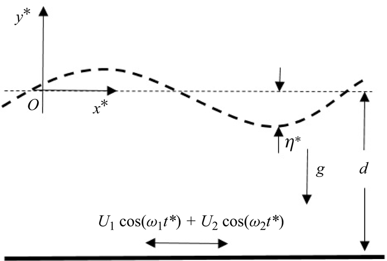
In the system of Cartesian coordinates $(x^{*},y^{*})$ (see figure 1), consider an incompressible Newtonian fluid film with density $\rho$, dynamic viscosity $\mu$ and thickness $d$ flowing on an oscillating horizontal wall whose law of displacement relative to a reference position is of the form $a_1 \sin (\omega _1 t^{*}) + a_2 \sin (\omega _2 t^{*})$, so that its velocity is given by

(2.1)

\begin{equation} \boldsymbol{U}_p^*(t^*)=U_p^*(t^*) \boldsymbol{x}^{*}=(U_{1}\cos(\omega_{1}t^{*})+ U_{2}\cos(\omega_{2}t^{*}))\boldsymbol{x}^{*}, \end{equation}

where $\boldsymbol {x}^{*}$ is the horizontal unit vector. The quantities $U_1=a_1 \omega _1$ and $U_2=a_2 \omega _2$ are the superimposed velocity amplitudes, while $\omega _{1}$ and $\omega _{2}$ are considered two incommensurable frequencies. Thus, the imposed oscillation consists of the superposition of two modes without the introduction of a phase shift. Each mode has its own frequency and amplitude.

Figure 1.

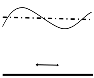
Newtonian fluid layer on an oscillating horizontal wall.

In the fixed frame, $(O,x^*, y^*)$, the system of the governing equations, is given by the following momentum and continuity equations:

(2.2)

$$\begin{gather} \rho\left(\frac{\partial }{\partial t^*}+\boldsymbol{V^*} \boldsymbol{\cdot} \boldsymbol{\nabla}\right)\boldsymbol{V^*}=-\boldsymbol{\nabla} P^*+\mu \Delta\boldsymbol{V^*}+\rho \boldsymbol{g}, \end{gather}$$

(2.3)

$$\begin{gather}\boldsymbol{\nabla} \boldsymbol{\cdot} \boldsymbol{V^*}=0. \end{gather}$$

Here $\boldsymbol {V}^*$ is the velocity field, $P^*$ is the hydrodynamic pressure, $\nu ={\mu }/{\rho }$ is the kinematic viscosity and $\boldsymbol {g}$ represents the acceleration due to gravity. The free surface of the fluid is described by $y^*=\eta (t^*,x^*)$, which represents the elevation of the interface with respect to its initial position coinciding with the axis $(O,x^*)$.

To non-dimensionalize the governing equations and boundary conditions, we introduce the following dimensionless variables:

(2.4a–e)

\begin{equation} t=\frac{t^*}{\omega_{1}^{-1}},\quad x=\frac{x^*}{d}, \quad y=\frac{y^*}{d},\quad \boldsymbol{V}=\frac{\boldsymbol{V}^*}{U_{1}},\quad {P}=\frac{{P}^*}{\rho U_1^{2}}.\end{equation}

For the characteristic scales, we have chosen the parameters of the first mode as we could have chosen those of the second mode. In addition, the choice of $1/\omega _1$ is representative of temporal variations more in accord with the linearization of convective acceleration terms leading to the equation governing the base flow in § 2.2. Also, the characteristic pressure is fixed by the disturbance problem, given that the base flow has a zero pressure gradient. Inserting (2.4a–e) into (2.2) and (2.3), we obtain the following dimensionless system:

(2.5)

$$\begin{gather} \left(\frac{2\beta^2}{Re}\frac{\partial }{\partial t}+\boldsymbol{V} \boldsymbol{\cdot} \boldsymbol{\nabla}\right)\boldsymbol{V}=-\boldsymbol{\nabla} P+\frac{1}{Re} \Delta\boldsymbol{V}-\frac{2\chi}{Re^2}\boldsymbol{y^*}, \end{gather}$$

(2.6)

$$\begin{gather}\boldsymbol{\nabla} \boldsymbol{\cdot} \boldsymbol{V}=\boldsymbol{0}. \end{gather}$$

Here $\boldsymbol {y^*}$ is an upward unit vector and $\beta =\sqrt {{\omega _1 d^2}/{2\nu }}$ is the dimensionless frequency parameter that represents the ratio of the average film thickness to the thickness of the Stokes layer induced by the wall oscillation, it is also interpreted as a measure of the relative oscillation frequency $\omega _1$. We recall that the Stokes layer is the one adjacent to the wall and entrained by the wall's oscillation. Its thickness, also known as the penetration depth of the viscous wave, is of the order of $\sqrt {{2\nu }/{\omega _1}}$. The other dimensionless numbers are: the Galileo number $\chi ={g d^3}/{2\nu ^{2}}$, which interprets the ratio of the gravity effect to the viscous effect; the Reynolds number, $Re={U_1 d}/{\nu }$, which measures the ratio of the inertial effect, due to the oscillation amplitude $U_1$, to the viscous effect. According to the choice of (2.4a–e), an interesting feature of these parameters is that the effects of frequency and amplitude modulation, which are the focus of this study, are measured only by $Re$ and $\beta$. Finally, it should be noted that the use of these characteristic scales also enables us to compare our results with those of Or (Reference Or1997).

The boundary conditions, in a dimensionless form are

(2.7a,b)

\begin{equation} U\vert_{y=-1}={U}_p(t),\quad V\vert_{y=-1}=0,\end{equation}

where $(U,V)$ are the dimensionless components of the velocity field $\boldsymbol {V}(x, y, t)$. The dimensionless velocity of the horizontal wall is given by

(2.8)

\begin{equation} {U}_p(t)=\cos(t)+\gamma\cos(\omega t), \end{equation}

where $\gamma ={U_2}/{U_1}$ is the ratio of superimposed velocity amplitudes and $\omega ={\omega _2}/{\omega _1}$ is the frequency ratio considered irrational. When the ratio of the velocity amplitudes is zero, we are in the configuration studied by Yih (Reference Yih1968), Or (Reference Or1997), Gao & Lu (Reference Gao and Lu2008). The boundary conditions at the free surface, $y=\eta (x,t)$, are the kinematic condition, the balance of tangential and normal stresses. The corresponding dimensionless equations are given as follows:

(2.9)

$$\begin{gather} V=\left(\frac{2\beta^2}{Re}\frac{\partial }{\partial t}+U\frac{\partial }{\partial x}\right)\eta, \end{gather}$$

(2.10)

$$\begin{gather}\frac{1}{\left(1+\left(\dfrac{\partial \eta}{\partial x}\right)^2\right)}\left[\left(\frac{\partial U}{\partial y}+\frac{\partial V}{\partial x}\right)\left(1-\left(\frac{\partial \eta}{\partial x}\right)^2\right)+2\left(\frac{\partial V}{\partial y}-\frac{\partial U}{\partial x}\right)\left(\frac{\partial \eta}{\partial x}\right)^2\right]=0, \end{gather}$$

(2.11)

\begin{gather} -p+P_o+\frac{2}{Re\left(1+\left(\dfrac{\partial \eta}{\partial x}\right)^2\right)}\left[\left(\frac{\partial V}{\partial y}+\frac{\partial U}{\partial x}\left(\frac{\partial \eta}{\partial x}\right)^2\right) -\left(\frac{\partial U}{\partial y}+\frac{\partial V}{\partial x}\right)\frac{\partial \eta}{\partial x}\right]\nonumber\\ \quad=\frac{1}{\varPsi Re^2}\frac{\dfrac{\partial^2 \eta}{\partial x^2}}{\sqrt{\left(1+\left(\dfrac{\partial \eta}{\partial x}\right)^2\right)^3}}. \end{gather}

The dimensionless parameter, $\varPsi ={\rho \nu ^2}/{d\sigma }$, is associated to the uniform surface tension $\sigma$ and measures the ratio of the viscous force to surface tension force, while $P_o$ is a dimensionless reference pressure at the interface.

2.2. Base flow

The basic state corresponds to a plane interface with a unidirectional velocity parallel to the $x$ axis, $\boldsymbol {V}_b=(U_b(y,t),0,0)$ and satisfying the following equation:

(2.12)

$$\begin{gather} 2\beta^2\frac{\partial U_b}{\partial t}=\frac{\partial^2 U_b}{\partial y^2}, \end{gather}$$

(2.13)

$$\begin{gather}0=-\frac{\partial \bar{P}}{\partial y}-\frac{2\chi}{Re^2}. \end{gather}$$

The boundary conditions of the base flow are

(2.14a,b)

\begin{equation} U_b\vert_{y=-1}={U}_p(t),\quad \left.\frac{\partial U_b }{\partial y}\right\vert_{y=0}=0. \end{equation}

It follows from (2.13) that the basic flow pressure is given by

(2.15)

\begin{equation} \bar{P}=P_o-\frac{2\chi}{Re^2}y,\end{equation}

where $\bar {P}=P_o$ is the interface pressure at $y=0$. The solution of (2.12) satisfying the boundary conditions (2.14a,b) is given by

(2.16)

\begin{equation} U_b=F_1(y)\cos(t)+F_2(y)\sin(t)+G_1(y)\cos(\omega t)+G_2(y)\sin(\omega t),\end{equation}

where

(2.17)

\begin{equation} \left.\begin{array}{c@{}} F_{1}=\dfrac{1}{2}\left[\dfrac{\cosh(r_{1}y)}{\cosh(r_{1})}+ \dfrac{\cosh(\overline{r_{1}}y)}{\cosh(\overline{r_{1}})}\right] \quad F_{2}=\dfrac{{\rm i}}{2}\left[\dfrac{\cosh(r_{1}y)}{\cosh(r_{1})}- \dfrac{\cosh(\overline{r_{1}}y)}{\cosh(\overline{r_{1}})}\right]\\ G_{1}=\dfrac{\gamma}{2}\left[\dfrac{\cosh(r_{2}y)}{\cosh(r_{2})}+ \dfrac{\cosh(\overline{r_{2}}y)}{\cosh(\overline{r_{2}})}\right] \quad G_{2}=\dfrac{{\rm i}\gamma}{2}\left[\dfrac{\cosh(r_{2}y)}{\cosh(r_{2})}- \dfrac{\cosh(\overline{r_{2}}y)}{\cosh(\overline{r_{2}})}\right] \end{array}\right\}, \end{equation}

with $r_{1}=(1+i)\beta, r_{2}=(1+i)\beta \sqrt {\omega }, \bar {r}_{1}$ and $\bar {r}_{2}$ are the complex conjugates of $r_{1}$ and $r_{2}$, respectively. Three parameters are involved in the expression of the base flow velocity profile: the ratio of the velocity amplitudes $\gamma$; the parameter $\beta = {d}/{\sqrt {{2\nu }/{\omega _1}}}={d}/{\delta _1}$, where $\delta _1$ is the thickness of the Stokes layer relative to $\omega _1$; and the parameter $\beta \sqrt {\omega }= {d}/{\delta _2}$, where $\delta _2$ is the thickness of the Stokes layer relative to $\omega _2$. Note that ${\delta _1}/{\delta _2}=\sqrt {\omega }$.

It is of great importance to identify the specific flow regimes that correspond to different frequency ratio ranges and to characterize the associated velocity profiles. In this context, figures 2 and 3 show the evolution of the base velocity profile, $U_b$, given by (2.16), respectively, for $\beta =3$ and $\beta =10$ and for different values of the frequency ratio.

Figure 2.

Time evolution of base velocity profiles for $\beta =3, \gamma =1$ and different frequency ratios over the time interval $[0,{\rm \pi} ]$.

Figure 3.

Time evolution of base velocity profiles for $\beta =10, \gamma =1$ and different frequency ratios over the time interval $[0,{\rm \pi} ]$.

For $\beta =3$, the velocity profiles show at $t=0$ zero velocities at positions much smaller than the fluid layer thickness, and therefore, the velocity at the interface is almost zero, except for $\omega ={1}/{\sqrt {37}}$. Note also that the thickness of the Stokes layer increases as the frequency ratio decreases. At $t={\rm \pi}$, the Stokes layers corresponding to low frequencies $\omega ={1}/{\sqrt {2}}$ and $\omega ={1}/{\sqrt {7}}$ also exhibit, as in the case $\omega ={1}/{\sqrt {37}}$, non-zero velocities at the interface, while for $\omega =\sqrt {2}, \omega =\sqrt {3}$ and $\omega =\sqrt {37}$, the Stokes layer thicknesses are notably less than that of the fluid layer.

For $\beta =10$, the interface velocities are zero and Stokes layer thicknesses are close to $y=-0.6$ for almost all frequency ratios. For $t =0$, velocity profiles reach their maximums at $y=-1$. Then, for $\omega =\sqrt {37}$, the maximum occurs at $y=-0.95$ for $t={{\rm \pi} }/{8}$ and the velocity profile inversion is complete for $t={\rm \pi}$.

These findings show that, depending on the parameter $\beta$ and the frequency ratio, two different regimes are observed in the base flow: one with a Stokes layer of thickness less than that of the fluid layer and one without. By varying the frequency ratio, the velocity profiles undergo significant changes in shape. These results contribute to a better understanding of the complex dynamics inside the fluid and effects of the different parameters on the velocity behaviour and subsequently on its stability.

At last, figure 4 shows the oscillating velocity of the fluid resulting from the wall oscillation. At $y=-1$, the quasi-periodic flow has a large amplitude that decreases as the free surface is approached.

Figure 4.

Time evolution of the base velocity profile for $\gamma =1, \beta = 3$ and for different locations: $y=-0.25,-0.5, -0.75,-1$.

2.3. Stability and normal modes analysis

The study of the linear stability of the base flow consists in superimposing on it infinitesimal perturbations by introducing the following variables:

(2.18a–d)

\begin{equation} U=U_b+u', \quad V=v', \quad P=\bar{P}+p', \quad \eta=\eta'.\end{equation}

Here $(u',v')$ are the components of the velocity disturbance in the Cartesian coordinates $(x,y)$, while $p^{'}$ and $\eta ^{'}$ designate pressure and interface disturbances, respectively. The two-dimensional perturbations satisfy the momentum and continuity equations (2.5) and (2.6):

(2.19)

$$\begin{gather} \frac{2\beta^2}{Re}\frac{\partial u'}{\partial t}+U_b\frac{\partial u'}{\partial x}+ v'\frac{\partial U_b}{\partial y}=-\frac{\partial p'}{\partial x}+\frac{1}{Re}\left(\frac{\partial^2 u'}{\partial x^2}+ \frac{\partial^2 u'}{\partial y^2}\right), \end{gather}$$

(2.20)

$$\begin{gather}\frac{2\beta^2}{Re}\frac{\partial v'}{\partial t}+U_b \frac{\partial v'}{\partial x}=-\frac{\partial p'}{\partial y}+\frac{1}{Re}\left(\frac{\partial^2 v'}{\partial x^2}+\frac{\partial^2 v'}{\partial y^2}\right), \end{gather}$$

(2.21)

$$\begin{gather}\frac{\partial u'}{\partial x}+\frac{\partial v'}{\partial y}=0. \end{gather}$$

The boundary condition on the oscillating wall located at $y=-1$ is now given by

(2.22)

\begin{equation} u'=v'=0.\end{equation}

The interfacial boundary conditions (2.9)–(2.11) are linearized by expanding all variables in the Taylor series near $y=0$, and retaining only the linear terms of this expansion in the resulting equations. Thus, the kinematic condition, the balance of tangential and normal stresses are written as follows:

(2.23)

$$\begin{gather} \frac{2\beta^2}{Re}\frac{\partial \eta'}{\partial t}=v'-U_b\frac{\partial \eta'}{\partial x}, \end{gather}$$

(2.24)

$$\begin{gather}\frac{\partial ^2 U_b}{\partial y^2}~\eta'+\frac{\partial u'}{\partial y}+ \frac{\partial v'}{\partial x}=0, \end{gather}$$

(2.25)

$$\begin{gather}\eta' \frac{\partial \bar{P}}{\partial y}+p'-\frac{2}{Re} \frac{\partial v'}{\partial y}+\frac{1}{\varPsi Re^2}\frac{\partial ^2 \eta}{\partial x^2}=0. \end{gather}$$

Taking the derivative of (2.25) with respect to the spatial variable $x$, we obtain

(2.26)

\begin{equation} \frac{\partial \eta'}{\partial x} \frac{\partial \bar{P}}{\partial y}+\frac{\partial p'}{\partial x}-\frac{2}{Re}\frac{\partial^2 v'}{\partial x\partial y}+\frac{1}{\varPsi Re^2}\frac{\partial ^3 \eta}{\partial x^3}=0, \end{equation}

where ${\partial p'}/{\partial x}$ can be found using (2.19) and the second boundary condition of (2.14a,b):

(2.27)

\begin{equation} \frac{\partial p'}{\partial x}=\frac{1}{Re}\left(\frac{\partial^2 u'}{\partial x^2}+ \frac{\partial^2 u'}{\partial y^2}\right)-\frac{2\beta^2}{Re}\frac{\partial u'}{\partial t}-U_b\frac{\partial u'}{\partial x}.\end{equation}

The perturbed streamfunction $\psi '$ is introduced:

(2.28a,b)

\begin{equation} u'= \frac{\partial \psi'}{\partial y},\quad v'=-\frac{\partial \psi'}{\partial x}.\end{equation}

Thereafter, the perturbations of the streamfunction, pressure and interface are written in normal modes, i.e.

(2.29)

\begin{equation} (\psi',p',\eta')= (\phi(y,t),p(y,t),h(t))\ {\rm e}^{{\rm i}k x},\end{equation}

where $k$ is the wavenumber of the perturbation amplitude considered to be real, since we are dealing with temporal stability. Substituting (2.29) into (2.19) and (2.20) and eliminating pressure, the Orr–Sommerfeld equation is derived:

(2.30)

\begin{align} &\left(\frac{2\beta^2}{Re}\frac{\partial }{\partial t}+{\rm i} k U_b\right) \left(\frac{\partial ^2 \phi }{\partial y^2}-k^2 \phi \right) -{\rm i} k\frac{\partial ^2 U_b}{\partial y^2}\phi\nonumber\\ &\quad=\frac{1}{Re}\left(\frac{\partial^4 \phi}{\partial y^4}-2 k^2 \frac{\partial^2 \phi}{\partial y^2}+k^4\phi\right). \end{align}

The boundary conditions (2.22), (2.23), (2.24) and (2.26) become

(2.31)

$$\begin{gather} \phi=\frac{\partial \phi}{\partial y}=0, \end{gather}$$

(2.32)

$$\begin{gather}\frac{2\beta^2}{Re}\frac{\partial h}{\partial t}=-{\rm i}k\phi-{\rm i}k U_b h, \end{gather}$$

(2.33)

$$\begin{gather}\frac{\partial^2\phi}{\partial y^2}+k^2\phi+U_{byy}h=0, \end{gather}$$

(2.34)

$$\begin{gather}\frac{2\beta^2}{Re}\frac{\partial^2\phi}{\partial t\partial y}-\frac{1}{Re}\left(\frac{\partial^2}{\partial y^2}-3 k^2\right)\frac{\partial\phi}{\partial y}+{\rm i} k U_b\frac{\partial\phi}{\partial y}+{\rm i} k\left(-\frac{2\chi}{Re^2}+\frac{1}{\varPsi Re^2}k^2\right)h=0. \end{gather}$$

3. Asymptotic solution in the long wavelength limit

The base flow solution $U_b$ is characterized by two incommensurate frequencies, $\omega _1$ and $\omega _2$. Here, the Floquet theory cannot be applied, however, we use the approximation that consists of rendering an irrational number, $\omega$, into a rational one. We therefore introduce the following variable changes:

(3.1a–c)

\begin{equation} \omega =\frac{p}{q},\quad \tau=\frac{t}{q},\quad \frac{\partial}{\partial t}=\frac{1}{q} \frac{\partial}{\partial \tau}.\end{equation}

Here $p$ and $q$ are prime integers (Boulal et al. Reference Boulal, Aniss, Belhaq and Rand2007, Reference Boulal, Aniss, Belhaq and Azouani2008; Yagoubi & Aniss Reference Yagoubi and Aniss2017); for instance, $\sqrt 2=\frac {1393}{985}, \sqrt 3=\frac {1351}{780}, \sqrt 5=\frac {2889}{1292}\cdots \sqrt {37}=\frac {882}{145}$. In the following, we introduce the variable changes:

(3.2a,b)

\begin{equation} \tau=\frac{t}{q}, \quad \frac{\partial}{\partial t}=\frac{1}{q} \frac{\partial}{\partial \tau}. \end{equation}

We search the solution of the system (2.30)–(2.34) in the form

(3.3a,b)

\begin{equation} \phi(y,\tau)=f(y,\tau)\ {\rm e}^{\lambda\tau}, \quad h(\tau)=\tilde{h}(\tau)\ {\rm e}^{\lambda\tau}, \end{equation}

where $f(y,\tau )$ and $\tilde {h}(\tau )$ are time-dependent functions and $\lambda$ is the Floquet exponent. For long wavelength perturbations, the wavenumber $k$ is considered as a small parameter and the form of the equations suggests looking for solutions in the power range of this small parameter:

(3.4a–c)

\begin{align} f={f}_o+k f_1+k^2 f_2+\cdots; \quad \tilde{h}=\tilde{h}_o+k \tilde{h}_1+k^2\tilde{h}_2+\cdots; \quad \lambda=\lambda_o+k \lambda_1+k^2\lambda_2+\cdots . \end{align}

In this study, the expansions are restricted to the order $k^2$, in order to compare our results with those by Yih (Reference Yih1968).

3.0.1. Order $k^0$:

At this order, the Orr–Sommerfeld equation (2.30) and the boundary conditions are then given by (2.31)–(2.34):

(3.5)

$$\begin{gather} \frac{\partial^4 f_o}{\partial y^4}- \frac{2\beta^2}{q}\frac{\partial^3f_o}{\partial \tau\partial y^2}- \frac{2\beta^2}{q}\lambda_o\frac{\partial^2f_o}{\partial y^2}=0, \end{gather}$$

(3.6)

$$\begin{gather}f_o=0, \quad \frac{\partial f_o}{\partial y}=0 \quad \text{at } y=-1, \end{gather}$$

(3.7)

$$\begin{gather}\frac{\partial^2f_o}{\partial y^2}+\frac{\partial^2U_b}{\partial y^2}\tilde{h}_o=0\quad \text{at } y=0, \end{gather}$$

(3.8)

$$\begin{gather}\frac{\partial^3f_o}{\partial y^3}-\frac{2\beta^2}{q}\frac{\partial^2f_o}{\partial \tau\partial y}-\frac{2\beta^2}{q}\lambda_o \frac{\partial f_o}{\partial y}=0 \quad \text{at }y=0, \end{gather}$$

(3.9)

$$\begin{gather}\frac{{\rm d} \tilde{h}_o}{d\tau}+\lambda_o \tilde{h}_o=0 \quad \text{at } y=0. \end{gather}$$

Since ${\tilde {h}}_{0}(\tau )$ is a time-periodic function of $\tau$, the kinematic condition (3.9) leads to an admissible solution $\lambda _o=0$. We choose $\tilde {h}_o=1$, otherwise, $\lambda _o \neq 0$ provides a damped Floquet mode demonstrated by Yih (Reference Yih1968), and this damped mode is of no interest here. Substituting the values of $\lambda _o$ and ${\tilde {h}}_{0}$ and solving (3.5)–(3.8), the first-order solution can be expressed as follows:

(3.10)

\begin{equation} f_o(y,\tau)=\Re\left[\frac{1-\cosh r_{1}(1+y)}{\cosh^2 r_{1}}\ {\rm e}^{{\rm i}q\tau}+\gamma\frac{1-\cosh r_{2}(1+y)}{\cosh^2 r_{2}}\ {\rm e}^{{\rm i}p\tau}\right]. \end{equation}

Obviously, $f_o(y,\tau )$ depends on the ratio of the amplitudes of the quasi-periodic modulation $\gamma ={U_2}/{U_1}$. When $\gamma =0$, the reduced solution (3.10) is identical to that of Yih (Reference Yih1968) when the characteristic scales are the same.

3.0.2. Order $k^1$:

At this order, the Orr–Sommerfeld equation and the boundary conditions are

(3.11)

$$\begin{gather} \frac{\partial^4f_1}{\partial y^4}-\frac{2\beta^2}{q}\frac{\partial^3f_1}{\partial \tau\partial y^2}= {\rm i} Re \left[U_b\frac{\partial^2f_o}{\partial y^2}-f_o\frac{\partial^2U_b}{\partial y^2}\right], \end{gather}$$

(3.12)

$$\begin{gather}f_1=0, \ \frac{\partial f_1}{\partial y}=0, \quad \text{at } y=-1, \end{gather}$$

(3.13)

$$\begin{gather}\tilde{h}_1\frac{\partial^2U_b}{\partial y^2}+\frac{\partial^2f_1}{\partial y^2}=0 \quad \text{at }y=0 , \end{gather}$$

(3.14)

$$\begin{gather}\frac{\partial^3f_1}{\partial y^3}-\frac{2\beta^2}{q}\frac{\partial^2f_1}{\partial \tau\partial y}={\rm i}ReU_b\frac{\partial f_o}{\partial y}+{\rm i}\frac{2\chi}{Re} \quad \text{at }y=0, \end{gather}$$

(3.15)

$$\begin{gather}\frac{2\beta^2}{q}\left(\frac{{\rm d} \tilde{h}_1}{d\tau}+\lambda_1\right)=-{\rm i} Re(f_o(0,\tau)+U_b(0,\tau)). \end{gather}$$

In (3.15), since $\lambda _1$ is a real number and $\tilde {h}_1$ is a time-periodic function, we have

(3.16)

$$\begin{gather} \lambda_1=0, \end{gather}$$

(3.17)

$$\begin{gather}\tilde{h}_1=\frac{Re}{r_{1}^2} \Im\left[\frac{{\rm e}^{{\rm i}q\tau}}{\cosh^2r_{1}}\right]+\gamma\frac{Re}{r_{2}^2} \Re\left[\frac{{\rm e}^{{\rm i}p\tau}}{\cosh^2 r_{2}}\right]. \end{gather}$$

The solution of (3.11) is written in the form

(3.18)

\begin{equation} f_1(y,\tau)=\psi_1(y)\ {\rm e}^{2 {\rm i}q\tau}+\psi_2(y)\ {\rm e}^{-2 {\rm i}q\tau}+\psi_3(y)\ {\rm e}^{2 {\rm i}p\tau}+\psi_4(y)\ {\rm e}^{-2 {\rm i}p\tau}+\psi_5(y). \end{equation}

3.0.3. Order $k^2$:

At this order, $\lambda _2$ is determined from the following equation:

(3.19)

\begin{equation} \frac{2\beta^2}{q}\left(\frac{{\rm d} \tilde{h}_2}{{\rm d} \tau}+\lambda_2\right)=-{\rm i} Re (f_1(0,\tau)+\tilde{h}_1U_b(0,\tau)). \end{equation}

Since $\lambda _2$ is a constant and $\tilde {h}_2$ a time-periodic function, we only need to determine $\psi _5(y)$. According to (3.11), we obtain

(3.20)

\begin{equation} \frac{\partial^4\psi_5(y)}{\partial y^4}= {\rm i} Re \left[U_b\frac{\partial^2f_o}{\partial y^2}-f_0\frac{\partial^2U_b}{\partial y^2}\right]. \end{equation}

The solution of this equation is written as

(3.21)

\begin{align} &\psi_5(y)=C_1y^3+C_2y^2+C_3y+C_4-{\rm i} Re\, \Re\left[\frac{\cosh r_{1}y(2+\cos r_{1}(1+y))}{4r_{1}^2\cosh r_{1}\cos^2 r_{1}}\right]\nonumber\\ &\quad -{\rm i} \gamma Re\, \Re\left[\frac{\cosh r_{2}y(2+\cos r_{2}(1+y))}{4r_{2}^2\cosh r_{2}\cos^2 r_{2}}\right], \end{align}

where

(3.22)

\begin{align} \left.\begin{array}{@{}c@{}} C_1={\rm i}\dfrac{\chi}{3Re},\\ C_2=0,\\ \displaystyle C_3=-{\rm i}\dfrac{\chi}{Re}-{\rm i} Re\, \Re\left[\dfrac{3\sinh r_{1}}{4r_{1}\cosh r_{1}\cos^2 r_{1}}\right]-{\rm i}\gamma^2 Re\, \Re\left[\dfrac{3\sinh r_{2}}{4r_{2}\cosh r_{2}\cos^2 r_{2}}\right]\\ \displaystyle C_4=-{\rm i}\dfrac{2\chi}{3Re}+{\rm i}Re\, \Re\left[\dfrac{3\cosh r_{1}-3r_{1}\sinh r_{1}}{4r_{1}^2\cosh r_{1}\cos^2 r_{1}}\right]+{\rm i}\gamma^2 Re\, \Re\left[\dfrac{3\cosh r_{2}-3r_{2}\sinh r_{2}}{4r_{2}^2\cosh r_{2}\cos^2 r_{2}}\right] \end{array}\right\}. \end{align}

The expression of $\lambda _2$ is obtained from (3.19):

(3.23)

\begin{equation} \lambda_2=\frac{q Re^2}{2\beta^2}\left[-\frac{2\chi}{3Re^2}+F(\beta)\right]. \end{equation}

Here

(3.24)

\begin{align} F(\beta)=\Re\left[\frac{3\cosh r_{1}-3r_{1}\sinh r_{1}-\cos r_{1}}{4r_{1}^2\cosh r_{1}\cos^2 r_{1}}\right] +\gamma^2 \Re\left[\frac{3\cosh r_{2}-3r_{2}\sinh r_{2}-\cos r_{2}}{4r_{2}^2\cosh r_{2}\cos^2 r_{2}}\right].\end{align}

The stability of the flow is determined by the sign of $\lambda _2$. For $\lambda _2<0$, the flow is stable and, for $\lambda _2>0$, it is unstable. In other words, the flow is stable if

(3.25)

\begin{equation} \frac{2\chi}{Re^2} < 3F(\beta). \end{equation}

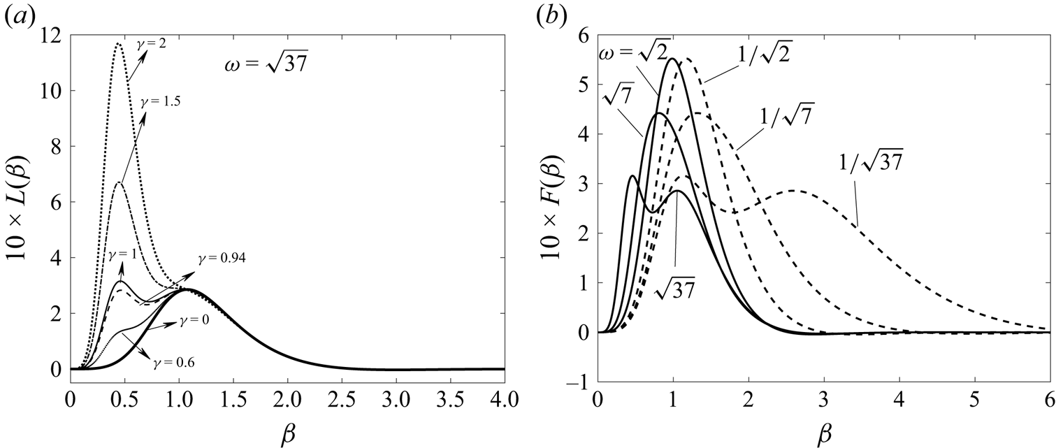
Figure 5(a,b) illustrates the variation of the function $10\times F(\beta )$ for different amplitude and frequency ratios $\gamma$ and $\omega$. Figure 5(a) indicates for $\omega = \sqrt {37}$ that the maximum of the function $10\times F(\beta )$ appears at one frequency, $\beta =1$, for $\gamma =0$ and $\gamma =0.6$. On the other hand, for $\gamma =1$, the maximum of the function appears at a low frequency, specifically at $\beta =0.461$, exhibiting an increase of the growth rate for longer wavelengths. The same is noted for $\gamma =1.5$ and $\gamma =2$ with a maximum for $\beta =0.441$. This observation suggests that the parameter $\gamma$ has a destabilizing influence on the $k\ll 1$ modes within the frequency range of $0\leq \beta \leq 2$. It is noteworthy that for $\gamma =0$ and $\beta =1$, the maximum value of the function $10\times F(\beta )$ is $2.78585$, which aligns precisely with the result obtained by Yih (Reference Yih1968) in the study of a Newtonian liquid on a horizontal wall subjected to periodic oscillation. Concerning the shape of the curves in figure 5(a), we note that for $\gamma = 0$, only the mode $F_1(y)\cos (t)+F_2(y)\sin (t)$ of the base flow (2.16), corresponding to the first mode of the wall oscillation, exists and its instability corresponds to studies by Yih (Reference Yih1968), Or (Reference Or1997), resulting in a single peak in the growth rate. As $\gamma$ gradually increases, the second mode, $G_1(y)\cos (\omega t)+G_2(y)\sin (\omega t)$, begins to coexist with the first, giving rise to instability with two peaks. Note that for $\gamma =1.5, 2$, the second mode dominates alone, again resulting in a single peak corresponding to the instability of the second mode and occurring for both values of $\gamma$ at $\beta =0.441$.

Figure 5.

Variation of the function $10 \times F(\beta )$, defined by expression (3.24), as a function of $\beta$, (a) for different values of $\gamma$, with $\omega =\sqrt 37$ and (b) for different values of $\omega$, with $\gamma =1$.

Figure 5(b) illustrates the impact of the frequency ratio, $\omega$, on the behaviour of the asymptotic function, $10\times F(\beta )$, versus the frequency parameter, $\beta$. The study focuses on various irrational values of $\omega$, namely $\sqrt {37}, \sqrt {7}, \sqrt {2}, {1}/{\sqrt {2}}, {1}/{\sqrt {7}}$ and ${1}/{\sqrt {37}}$. Surprisingly, the evolution of the asymptotic function reveals that its maximum has the same value when the horizontal wall is excited by the frequency ratio $\omega$ or by its inverse. The same maximum of the asymptotic function is obtained for $\omega$ and $1/\omega$ but for two different values of the frequency parameter. 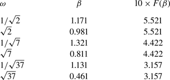For instance, for $\omega =\sqrt {2}$ and $\omega ={1}/{\sqrt {2}}$, the maximum is $5.521$ at $\beta =0.981$ and $\beta =1.171$, respectively. Additionally, the findings presented in table 1 further corroborate the consistent behaviour of the asymptotic function for the specific excitation cases explored in the study.

Table 1.

The maximum of the evolution of the analytical function $10\times F(\beta )$ when $\gamma =1, \chi =1$ and $\varPsi = 0.05$.

To explain the shift in figure 5(b) when taking the inverse frequency ratio, note that $\omega _1$ and $\omega _2$ play the same role. Thus, we can switch from the system (2.30)–(2.34) in $\omega$ to a system in $1/\omega$ using the change of variable $\omega t= \tau$. From here, we show that the parameter ${\beta }_{1/\omega }$ corresponding to the frequency $1/\omega$ is linked to the parameter ${\beta }_{\omega }$ by the relation ${{\beta }^2_{1/\omega }}=\omega {\beta }^2_{\omega }$. This relationship is verified by the results obtained numerically in table 1. For instance, knowing that $\beta _\omega =0.981$ for $\omega =\sqrt {2}$, we calculate ${{\beta }_{1/\sqrt {2}}}=\sqrt {\sqrt {2} {\beta }^2_{\omega }}=1.17$ to find the same value as in table 1. The same applies to the other frequency ratios.

4. Numerical procedure for arbitrary wavenumber

4.1. Spatial discretization

The numerical solution of the problem (2.30)–(2.34) allows us to determine the control parameters $Re$ and $k$ describing the stability diagram relative to the system's instability threshold for different frequency ratios. The Chebyshev collocation spectral method (Trefethen Reference Trefethen2000; Weideman & Reddy Reference Weideman and Reddy2000; Canuto et al. Reference Canuto, Hussaini, Quarteroni and Zang2007) is used to treat spatial dependence by decomposing the elements of a space vector onto a basis of Lagrangian functions $L_j(y)$. Thus, the solution of the Orr–Sommerfeld equation (2.30) is approximated by a Lagrange polynomial series expansion:

(4.1)

\begin{equation} \phi(y,t)=\sum^{N}_{j=1} \phi_{j}(t)L_{j}(y),\quad j=1,\ldots,N. \end{equation}

The functions $\phi _{j}(t)$ are unknown amplitudes depending on time and $L_{j}(z)$ are the fundamental polynomials of Lagrange defined as

(4.2)

\begin{equation} L_{j}(y)=\prod^{N}_{l=0,l\neq j} \left(\frac{y-y_{l}}{y_{j}-y_{l}}\right),\quad j=1,\ldots N. \end{equation}

The interpolant polynomials $\phi _{j}(t)$ satisfy exactly the solutions in $N$ collocation points $y_l$ such that

(4.3)

\begin{equation} L_j(y_l)=\delta_{lj},\quad j=1,\ldots,N, \end{equation}

where $\delta _{lj}$ is the Kronecker symbol. The collocation points are the extrema of the Chebyshev polynomial of order $N$ defined as

(4.4)

\begin{equation} T_N(y)=\cos(N\cos^{-1}(y)). \end{equation}

This polynomial admits exactly $N$ extrema. These are Chebyshev–Gauss– Lobatto points, defined in the interval $[-1, 1]$ and written as

(4.5)

\begin{equation} {y}_l=\cos\left(\frac{{\rm \pi}(l-1)}{N-1}\right)\quad l=1,\ldots,N. \end{equation}

Lagrange's interpolation polynomials are then written for the case of Chebyshev–Gauss–Lobatto collocation points:

(4.6)

\begin{equation} L_{j}(y)=\frac{(-1)^{j}(y^{2}-1)T'_{N}(y)}{\bar{c}_{j}(N-1)^{2}(y-y_{j})}. \end{equation}

Here ${\bar {c}}_1={\bar {c}}_N=2$ and ${\bar {c}}_2=\cdots ={\bar {c}}_{N-1}=1$. The derivatives of order $n$ of the functions $\phi (y,t)$ with respect to $y$, evaluated at $N$ collocation points, are expressed in terms of matrices $D^{n}_{lj}$ of size $n \times n$, whose indices $l$ and $j$ denote their rows and columns, respectively:

(4.7)

\begin{equation} \frac{\partial^{n}}{\partial y^{n}}\phi(y_{i},t)=\sum^{N}_{j=0}\phi_{j}(t)L^{n}_{j}(y_i)= \sum^{N}_{j=0}\phi_{j}(t)D^{n}_{ij}. \end{equation}

The components of the matrices $D^{n}_{lj}$ are the derivatives of order $n$ of the basic functions of Lagrange taken in each of the collocation points. The matrix derived from first order $D_{lj}$ calculated at the collocation points of Chebychev–Gauss–Lobatto is written explicitly in this form:

(4.8)

\begin{align} D_{lj}=\left\{\begin{array}{@{}ll@{}} \dfrac{\bar{c}_l(-1)^{l+j}}{\bar{c}_j(y_l-y_j)}, & j\neq l, \\ -\dfrac{y_j}{2(1-y_j^2)}, & j=l\neq 1,N, \\ \dfrac{2(N-1)^2+1}{6}, & j=l=1, \\ -\dfrac{2(N-1)^2+1}{6}, & j=l=N. \\ \end{array}\right. \end{align}

Since the problem formulation was established in the interval $[-1,0]$ and the Chebychev collocation points are defined in the interval $[-1, 1]$, the variable $y$ and the derivatives are respectively replaced in the numerical procedure by $\tilde {y}=2y+1$ and $2^n ({\partial ^n}/{\partial \tilde {y}^n})$. After that, by introducing (4.1) into (2.30) and evaluating at the collocation points $\tilde {y}_j$, we obtain

(4.9)

\begin{align} \left[\frac{2\beta^2}{Re}(4D_{lj}^2-k^2 I_{lj})\right] \left[\frac{\partial \phi_{j}}{\partial t}\right] &= \left[\frac{1}{Re}16D_{lj}^4-\left[\frac{2 k^2}{Re}+{\rm i} k U_b\right] 4D_{lj}^2 \right.\nonumber\\ &\quad + \left.\left[\frac{k^4}{Re}+ {\rm i} k^3 U_{blj} + {\rm i} k U_{blj,\tilde{y}\tilde{y}}\right]I_{lj}\right][\phi_{lj}], \end{align}

where $l$ $= 3, 4,\ldots, N-2$; $j =1$,…, $N$ and $I_{i,j}$ are the coefficients of the identity matrix. The boundary conditions are evaluated at the collocation points, $\tilde {y}= 1$ and $\tilde {y}=-1$:

(4.10)

$$\begin{gather}{}[I_{Nj}][\phi_{j}]=0, \end{gather}$$

(4.11)

$$\begin{gather}{}[2D_{Nj}][\phi_{j}]=0, \end{gather}$$

(4.12)

$$\begin{gather}{}[2\beta^{2} D_{1j}]\left[\frac{\partial \phi_{j}}{\partial t}\right]=\left[(8 D_{1j}^3-6 k^2D_{1j}-2{\rm i} k Re U_b D_{1j}), -\frac{1}{R}\left(2\chi+\frac{k^2}{\varPsi}\right){\rm i} k\right]\begin{bmatrix} \phi_{j} \\ h \end{bmatrix}, \end{gather}$$

(4.13)

$$\begin{gather}{}[4D_{1j}^2+ k^2 I_{1j}, U_{b,\tilde{y}\tilde{y}}]\begin{bmatrix} \phi_{j} \\ h \end{bmatrix}=0, \end{gather}$$

(4.14)

$$\begin{gather}{}[0 , 2\beta^2I_{1j}]\begin{bmatrix} \dfrac{\partial \phi_{j}}{\partial t} \\ \dfrac{\partial h}{\partial t} \end{bmatrix}=[-{\rm i} k Re I_{1j} , -{\rm i} k Re U_{b}]\begin{bmatrix} \phi_{j} \\ h \end{bmatrix}. \end{gather}$$

Thus, we obtain a square system of dimension $(N+1)\times (N+1)$, which is written in the form

(4.15)

\begin{equation} \boldsymbol{B}\frac{\partial \boldsymbol{x}}{\partial t}=\boldsymbol{M}(t)\boldsymbol{x}, \end{equation}

where $\boldsymbol {x}(t)=(\phi _{1},\phi _2,\ldots,\phi _{N},h)^T$ and $\boldsymbol {M}(t)=\boldsymbol {M}_{o}+\boldsymbol {M}_{s1} \sin (t)+\boldsymbol {M}_{c1}\cos (t)+ \boldsymbol {M}_{s2}\sin (\omega t)+\boldsymbol {M}_{c2}\cos (\omega t)$. Note that $\boldsymbol {B}, \boldsymbol {M}_{o}, \boldsymbol {M}_{c1}, \boldsymbol {M}_{s1}, \boldsymbol {M}_{c2}$ and $\boldsymbol {M}_{s2}$ are matrices with constant coefficients defined from the system of (4.9)–(4.14).

4.2. Floquet analysis

To solve the system of (4.15) in time, the changes of variables given by (3.1a–c) are used to obtain a Floquet system:

(4.16)

\begin{equation} \frac{\boldsymbol{B}}{q} \frac{\partial \boldsymbol{x}}{\partial \tau}=(\boldsymbol{M}_{o}+\boldsymbol{M}_{s1}\sin(q \tau)+\boldsymbol{M}_{c1}\cos(q \tau)+\boldsymbol{M}_{s2}\sin(\,p \tau)+\boldsymbol{M}_{c2}\cos(\,p \tau))\boldsymbol{x}. \end{equation}

Floquet's theory (Nayfeh & Mook Reference Nayfeh and Mook2008) is now applied to the discretized matrix system (4.15), which is periodic in time. This theory states that there exists a constant matrix $\boldsymbol {R}$ such that

(4.17)

\begin{equation} \boldsymbol{S}(t+T)=\boldsymbol{R}\boldsymbol{S}(t),\end{equation}

with $\boldsymbol {S}$ the fundamental matrix of the system (4.15), which satisfies

(4.18)

\begin{align} \frac{1}{q} \boldsymbol{B}\frac{\partial \boldsymbol{S}}{\partial t}=(\boldsymbol{M}_{o}+\boldsymbol{M}_{s1}\sin(q \tau)+\boldsymbol{M}_{c1}\cos(q \tau)+\boldsymbol{M}_{s2}\sin(\,p \tau)+\boldsymbol{M}_{c2}\cos(\,p \tau))\boldsymbol{S}.\end{align}

In addition, if the eigenvalues of the matrix $\boldsymbol {R}$ are $\lambda _i$, the solution of (4.16) can be written as

(4.19)

\begin{equation} x_i=Z_i(t)\exp(\lambda_i t), \end{equation}

where $\boldsymbol {Z}(t)$ is a periodic function of period $T$ and the coefficients $\lambda _i$ are the Floquet exponents that are related to the eigenvalues $\gamma _i$ by the relationship:

(4.20)

\begin{equation} \lambda_i=\frac{1}{T}\ln(\gamma_i). \end{equation}

To obtain $\boldsymbol {R}$, the system (4.18) is integrated in time using a fourth-order Runge–Kutta numerical scheme with the initial condition $\boldsymbol {S}(T)=\boldsymbol {R}~\boldsymbol {S}(0)$, where $\boldsymbol {S}(0)=\boldsymbol {I}$ is the matrix identity. After determining the eigenvalues $\gamma _i$ of $\boldsymbol {R}$, the coefficients $\lambda _i$ are calculated using relation (4.20).

The marginal stability curves $Re(k)$ are determined for a given set of flow parameters ($\beta, \chi, \varPsi, \gamma, \omega, k)$, by incrementing $Re$ from an initial value $Re_0$ until the value of $Re$ is identified for which the growth rate, the largest real part of $\lambda _i$, crosses zero for the first time. The value of $Re$ is then refined using the Newton–Raphson method. Once the $Re(k)$ curve is determined, the critical Reynolds number and wavenumber correspond to the minimum of this curve.

5. Validation of the numerical procedure

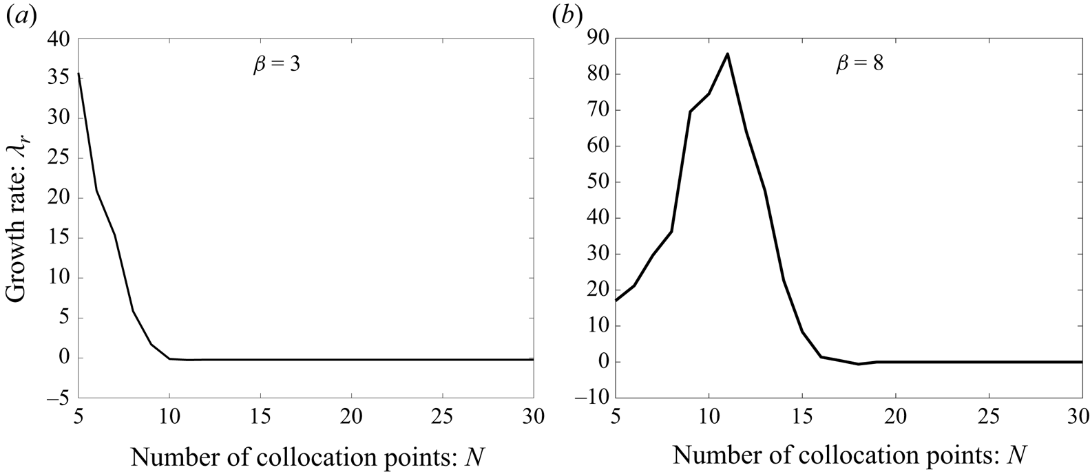
The convergence of the numerical procedure was examined by determining the evolution of the growth rate, $\lambda _r$, as a function of the number of collocation points $N$. Here $\lambda _r$ is considered to correspond to the most dangerous mode and represents the largest real part of the Floquet exponent, $\lambda _i$. This evolution is illustrated in figure 6 for $\omega =\sqrt {37}$ and $\gamma =1$ in the presence of gravity $\chi =1$ and when the viscosity effects are negligible compared with the surface tension forces, $\varPsi =0.05$. Figure 6(a) is obtained for $(\beta =3, Re=100)$ and figure 6(b) for $(\beta = 8, Re=5000)$. We note that for $N=17$, the numerical results no longer vary significantly and we can therefore consider that, for $\beta \leq 8$, the number of collocation points is $N=20$, and for $\beta > 8$, is $N=30$, as well as the range of Reynolds numbers $Re$ to be determined, are sufficient to obtain results with good accuracy.

Figure 6.

Convergence of the growth rate $\lambda _r$ as a function of the number of Chebychev collocation points $N$ for the cases (a) $\beta =3, Re=100$ and (b) $\beta =8, Re=5000$, with $\omega =\sqrt {37}, \chi =1 , \varPsi =0.05$ and $\gamma =1$.

The accuracy of the numerical results was also confirmed by comparing them with the asymptotic solution obtained, in § 3, in the long wavelength limit. According to expression (3.23), for $k\ll 1$, the eigenvalues dominating the flow stability are characterized by the Floquet parameter, $\lambda =\lambda _o+k \lambda _1+k^2\lambda _2+\cdots$, where $\lambda _o=\lambda _1=0$. 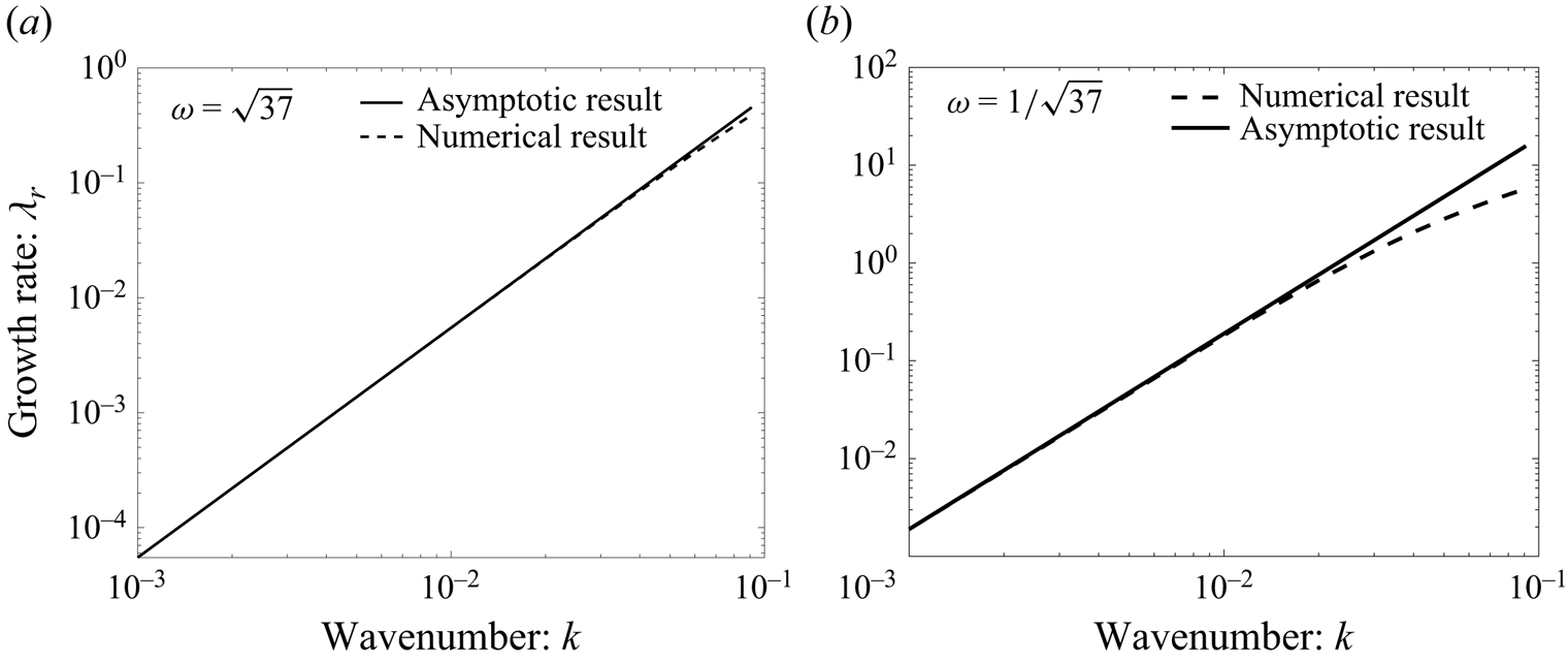Figure 7 shows the variation of $\lambda _2$ and that of the real part of $\lambda$, namely $\lambda _r$, as a function of $k$ for the periodic case $(\gamma =0)$ and for $\beta =2$ and $Re=50$. Excellent agreement between numerical results and theoretical predictions is observed, particularly for $k < 4\times 10^{-2}$. In the situation of two frequencies $(\gamma \neq 0)$, a comparison between numerical and analytical results for long wavelengths is presented in table 2.

Figure 7.

Comparison of asymptotic and numerical growth rates for (a) $\omega =\sqrt {37}$ and (b) $\omega =1/\sqrt {37}$ for $\beta =2, Re=50, \chi =1, \varPsi = 0.05$ and $\gamma =0$.

Table 2.

Comparison between analytical results at long wavelengths and numerical results with $\omega ={\omega _2}/{\omega _2}=1, \chi =1$ and $\varPsi = 0.05$.

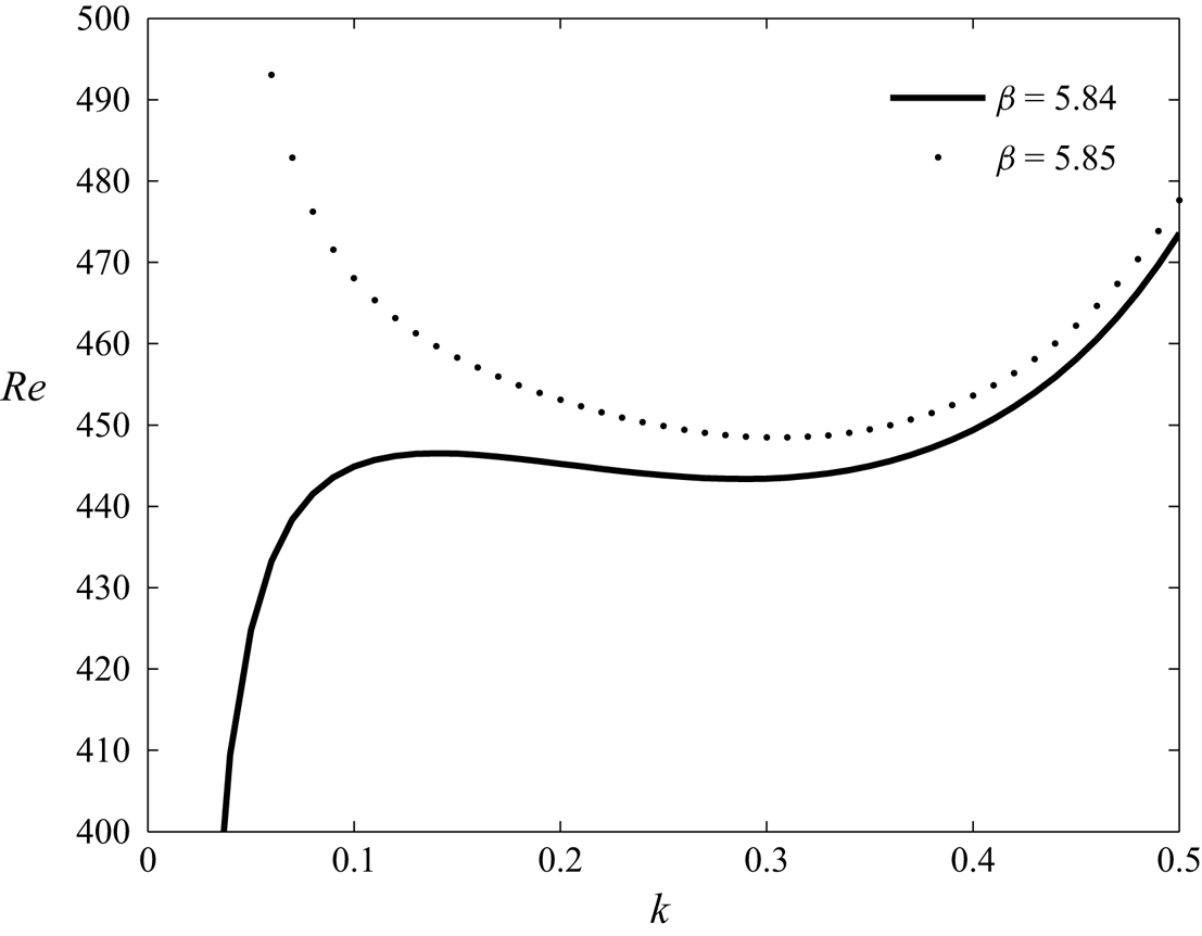
At last, the numerical results are also validated by comparing them with those obtained by Gao & Lu (Reference Gao and Lu2008) who considered periodic oscillation of the horizontal wall, $\gamma =0$, with $\chi =0, \varPsi =0.05$. Thus, figure 8 confirms that our numerical results coincide exactly with those obtained by Gao & Lu (Reference Gao and Lu2008) who showed that for $\beta =5.84$, the marginal stability curve is without threshold and the disturbances are long wavelengths, whereas for $\beta =5.85$, the marginal stability curve admits a threshold and instability is finite wavelength.

Figure 8.

Marginal stability curves for $\chi =0, \varPsi =0.05$ and $\gamma =0$. Instability without threshold (long wavelength) for $\beta =5.84$ and with threshold (finite wavelength) for $\beta =5.85$.

6. Results and discussion

The main results discussed here concern the effects of modulation frequency and amplitude ratios on flow stability in a layer of Newtonian fluid driven by a horizontal wall subjected to quasi-periodic oscillations ($\gamma \neq 0$ and $\omega$ is irrational). The characteristics of the fluid used (water–air interface) are: $\rho =10^3\ \textrm {kg}\ \textrm {m}^{-3},\ g=9.81\ \textrm {m}\ \textrm {s}^{-2}$ and $\sigma =30\times 10^{-3}\ \textrm {N}\ \textrm {m}^{-1}$. These physical properties of the liquid lead to a reasonable range of dimensionless parameters (Or Reference Or1997); for example, $\varPsi ={\rho \nu ^2}/{d\sigma }=0.05$ and $\chi ={gd^3}/{2\nu ^2}=1$.

6.1. Influence of the frequency ratio, $\omega ={\omega _2}/{\omega _1}$, on the marginal stability curves: $(Re,k)$

In figure 9, marginal stability curves, Reynolds number $Re={U_1d}/{\nu }$ versus the wavenumber $k$, are shown for the frequency parameter, $\beta =3.5$, the ratio of the characteristic modulation velocities, $\gamma ={U_2}/{U_1}=1$, and for several frequency ratios, $\omega =\sqrt {37}, \sqrt {7}, \sqrt {2}, {1}/{\sqrt {2}}, {1}/{\sqrt {7}}$ and ${1}/{\sqrt {37}}$. The results show that as $\omega$ decreases, the instability threshold shifts progressively to the left with a significant decrease in the critical wavenumber, which is therefore in the region of long wavelength perturbations. This is accompanied by a destabilizing effect that results in a significant decrease in the critical Reynolds number, $Re_c$. For very small values of the frequency ratio, as can be seen in figure 9(e,f), instability is associated with long wavelength disturbances, $k_c = 0$ and, thus, it is homogeneous. For intermediate or very large values of $\omega$ (see figure 9a–d), the instability is inhomogeneous or thresholded, $k_c \neq 0$, i.e. the perturbations are associated with finite wavelengths.

Figure 9.

Effect of the frequency ratio, $\omega$, on marginal stability curves for $\chi =1 , \varPsi =0.05, \beta =3.5$ and $\gamma =1$, (a) $\omega =\sqrt {37}$, (b) $\omega =\sqrt {7}$, (c) $\omega =\sqrt {2}$, (d) $\omega =1/\sqrt {2}$, (e) $\omega =1/\sqrt {7}$ and (f) $\omega =1/\sqrt {37}$.

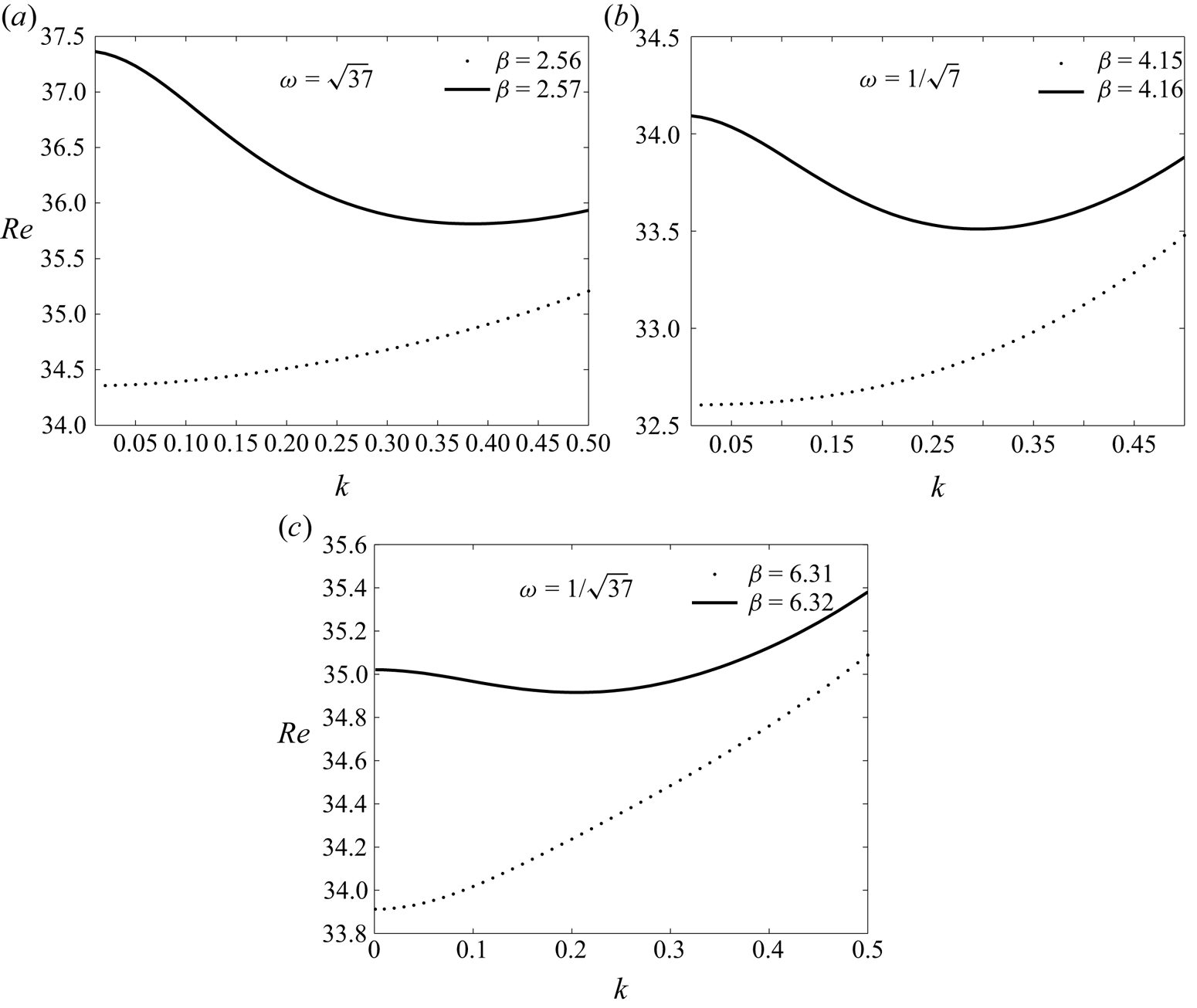
The marginal stability curves, in the $(Re,k)$ plane, shown in figure 10 aim to identify the $\beta$ frequency parameter for which there is a transition between instabilities with and without thresholds for different frequency ratios. For instance, in figure 10(a), if the imposed frequency remains slightly below $\beta =2.57$, this case corresponds to the lower neutral curve with a local minimum at $k=0$, i.e. in the long wavelength regime. In this situation, results indicate that the long-wave mode is more unstable than the finite-wave mode. On the contrary, for $\beta =2.57$, the neutral curve has a threshold with finite wavelength. For the neutral curves with a threshold, the local minimum shifts towards the long wavelength zones as the frequency ratio, $\omega$, decreases. Indeed, numerical results give $k = 0,38\ (Re=35.80)$ for $\omega =\sqrt {37}, k = 0,3\ (Re=33.51)$ for $\omega ={1}/{\sqrt {7}}$ and $k = 0,2\ (Re=34.91)$ for $\omega ={1}/{\sqrt {37}}$.

Figure 10.

Marginal stability curves corresponding to the branch points for $\chi =1 , \varPsi =0.05$ and $\gamma =1$.

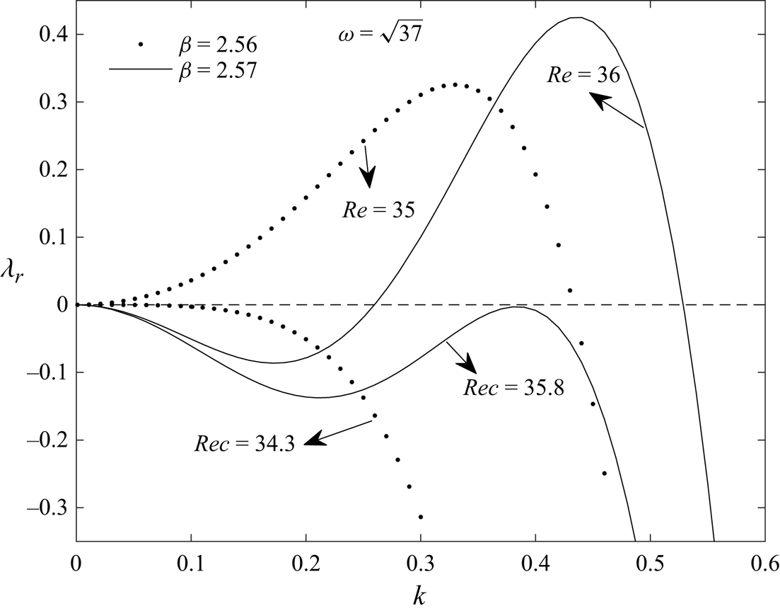
To consolidate the findings of figure 10(a) on long wavelength and finite wavelength instabilities, we present in figure 11 the growth rate defined at the beginning of § 5 as a function of the wavenumber $k$ for $\beta =2.56$ and $\beta =2.57$. For Reynolds numbers below their critical values given in figure 10(a) ($Re=34.3$ for $\beta =2.56$ and $Re=35.8$ for $\beta =2.57$), the growth rate is negative and we are in a stable configuration. However, for Reynolds numbers slightly above their critical values ($Re=35$ for $\beta =2.56$ and $Re=36$ for $\beta =2.57$), we note that for $\beta =2.6, \lambda _r$ is positive for wavenumbers between $k=0$ and $k=0.43$, and therefore, long wavelength instability occurs in the vicinity of $k =0$. However, for $\beta =2.7, \lambda _r$ is positive for values of $k$ between $0.26$ and $0.43$, which means that instability occurs for finite wavenumbers, and therefore, wavelengths too.

Figure 11.

Growth rate $\lambda _r$ versus the wavenumber $k$ for $\chi =1 , \varPsi =0.05$ and $\gamma =1$. Here $\beta =2.56$ corresponds to long wavelength instability and $\beta =2.57$ corresponds to finite wavelength instability.

At last, we note that the frequency parameter below which there is no threshold instability and above which there is threshold instability increases with decreasing frequency ratio. These results therefore confirm that the frequency ratio plays an important role in the appearance of one type of instability or another, and also in the selection of the wavenumber, i.e long wavelength or finite wavelength.

6.2. Influence of the frequency ratio, $\omega ={\omega _2}/{\omega _1}$, on the instability threshold in the plane ($Re_c,\beta$) and ($k_c,\beta$)

In this section, attention is focused on the curves representing the critical Reynolds number, $Rec$, and the critical wavenumber, $k_c$, as a function of the frequency parameter, $\beta$ ($0\leq \beta \leq 10$), for different frequency ratios, $\omega$: (a) $\omega =\sqrt {37}$, (b) $\omega =\sqrt {7}$, (c) $\omega =\sqrt {2}$, (d) $\omega =1/\sqrt {2}$, (e) $\omega =1/\sqrt {7}$ and (f) $\omega =1/\sqrt {37}$. The discussion here focuses on the influence of the frequency ratio on the stability diagrams in the ($Re_c,\beta$) plane as well as in the ($k_c,\beta$) plane, while adopting the $\beta$ frequency interval ($0\leq \beta \leq 10$) considered by Yih (Reference Yih1968) and Or (Reference Or1997) for comparison purposes.

6.2.1. Stability diagram in the plane $(Rec, \beta )$

In figure 12 the stable and unstable regions are denoted by S and U, respectively. The limits of long wavelengths are indicated by vertical dotted lines, the limits of finite wavelengths are indicated by oblique lines. The solid lines represent the variation of the critical Reynolds number $Re_c$, while the dashed lines do not represent a criticality because of the domination of long wavelengths.

Figure 12.

Effect of the irrational frequency ratio on the stability diagram in the $(Rec, \beta )$ plane. Evolution of the critical Reynolds number $Rec$ versus the frequency parameter $\beta$ for several frequency ratios, $\omega$, and for $\chi =1, \varPsi =0.05$ and $\gamma =1$. The boundaries of long wavelengths are denoted by the vertical dotted lines, the boundaries of finite wavelengths are denoted by the oblique lines. The solid lines represent the variation of the critical Reynolds number $Rec$, while the dashed lines do not represent a criticality because of the domination of long wavelengths.

For $\omega =\sqrt {37}$, three neutral U-shaped curves appear in different intervals of $\beta$, corresponding to $k=0$ (long wavelength instability). These intervals, in order, are as follows: $0\leq \beta \leq 2.63, 4.25\leq \beta \leq 5.84$ and $7.42\leq \beta \leq 8.99$. They agree satisfactorily with those by Or (Reference Or1997) in the presence of gravity $\chi =1$ and for $\psi =0.05$. This agreement with the case of periodic oscillation (Or Reference Or1997) occurring here for a large frequency ratio has been noted in other previous works (Boulal et al. Reference Boulal, Aniss, Belhaq and Rand2007, Reference Boulal, Aniss, Belhaq and Azouani2008; Yagoubi & Aniss Reference Yagoubi and Aniss2017). In this context, as $\beta$ increases from long wavelength unstable intervals, three oblique curves, corresponding to finite wavelength stability limits, bifurcate into straight lines at points $P_1, P_2$ and $P_3$ for the values of $\beta$ shown in table 3. This behaviour indicates that, within a range of the frequency parameter, one branch can continue with a critical Reynolds number corresponding to long wavelength disturbances $(k\longrightarrow 0)$, while another branch can emerge by changing the frequency parameter and the disturbances become associated with finite wavelengths $(k\neq 0)$, in other words instability has a threshold. Note that the finite wavelength neutral curves, indicated by continuous oblique lines, emerge from the branching points and grow monotonically until they intersect the next U-shaped neutral curve related to a no-threshold instability. The long-wave perturbations revert to being the physically preferred perturbations, although finite-wave instability can also occur for a sufficiently large Reynolds number above the solid curves.

Table 3.

Effect of the frequency ratio, $\omega$, on the branch points $P1, P2$ and $P3$, with $\gamma =1, \chi =1$ and $\varPsi =0.05$.

When the frequency ratio decreases to $\omega =\sqrt {7}$ in figure 12(b), the intervals of long wavelength instabilities have not undergone a noticeable change compared with the $\omega =\sqrt {37}$ case. Moreover, in the first U-shaped curve, the most unstable mode corresponds to the lowest critical Reynolds number $Re=2.127$ for $\beta =0.8$ whereas, for $\omega =\sqrt {37}$, it corresponds to $Re=2.517$ for $\beta =0.46$, meaning a weakly destabilizing effect. The findings made on $\omega = \sqrt {7}$ can also be made on $\omega = \sqrt {2}$ where the most unstable mode occurs for $Re= 1.903$ for $\beta =0.981$.

The shift from $\omega =\sqrt {2}$ to $\omega ={1}/{\sqrt {2}}$ is accompanied by the disappearance of the third oblique branch where instability is threshold. In addition, the branching points $P_1$ and $P_2$ become located for larger values of $\beta$ (see table 3). Similarly, the U-shaped instability undergoes translations, for instance, the third U zone undergoes a translation towards larger values of the frequency parameter, i.e. $8.82 \leq \beta \leq 10$. The last observation we make concerns the destabilizing effect described in the frequency band of the first U-shaped branch occupying a wider $0\leq \beta \leq 2.99$ interval, where long wavelength instability is potential this time at $Re=1.903$ and $\beta =1.171$.

When passing from $\omega ={1}/{\sqrt {2}}$ to $\omega ={1}/{\sqrt {7}}$, the third U-shaped curve disappears completely and the first widens considerably to occupy an even wider interval $[0, 4.285]$ with this time a stabilizing effect where the potential instability takes place at $Re=2.127$ and $\beta =1.3$.

Switching to $\omega ={1}/{\sqrt {37}}$ there is a total suppression of the second U-shaped curve while the first one widens again and takes place on the interval of the frequency parameter $[0, 6.496]$, and there is potential instability for long wavelengths at $Re=2.517$ and $\beta =1.145$. In parallel, the finite wavelength instability occupies the interval of the frequency parameter $[6.32, 10]$ in figure 12(e). Note that in figure 12 the deformation of the neutral curves in the vicinity of the onset for $\omega =\sqrt {37}$ and $\omega =1/\sqrt {37}$ in fact shows two minima, each of which represents a potential instability of one of the two modes of the base flow. This is explained by the results of the asymptotic study presented in figure 5(b), where we note that for $\sqrt {37}$ and ${1}/{\sqrt {37}}$, there are two growth rate maxima, each associated with a mode of the base flow.

In summary, the sensitivity of stability to variations in frequency ratio thus underlines the need for a comprehensive understanding of system response, particularly in scenarios involving complex frequency-dependent dynamics. The numerical results show that reducing the frequency ratio, $\omega$, from $\sqrt {37}$ to ${1}/{\sqrt {37}}$ leads to an enlargement of the long-wave and finite-wave instability zones, which also undergo a translation towards intervals of large $\beta$ values. Furthermore, for $\omega ={1}/{\sqrt {37}}$, only the main branch in ${\rm U}$ and the first oblique branch occupy the entire frequency parameter interval $[0, 10]$.

6.2.2. Stability diagram in the plane $(k_c, \beta )$

The evolution of the instabilities with and without threshold with the frequency ratio described above is accompanied above all by the evolution of the critical wavenumber of the finite wavelength instability in figure 13.

Figure 13.

Variation of the wavenumber $k _{c}$ (finite wavelength instability) as a function of the parameter $\beta$, for $\chi =1 , \varPsi =0.05$ and $\gamma =1$.

Interesting observations can be made when examining the case of $\omega =\sqrt {37}$ as illustrated in figure 13(a). On the one hand, these findings are consistent with those by Or (Reference Or1997) and Yih (Reference Yih1968). Indeed, we have already pointed out in the section above that for large frequency ratios, stability diagrams seem to resemble the periodic case and this behaviour was also observed in earlier works (Boulal et al. Reference Boulal, Aniss, Belhaq and Rand2007, Reference Boulal, Aniss, Belhaq and Azouani2008; Yagoubi & Aniss Reference Yagoubi and Aniss2017). The behaviour of the critical wavenumber $k_c$ along the different branches unveils intriguing dynamics. Specifically, within the context of the first oblique branch, a very pronounced growth in $k_c$ spanning the range from $k_c=0.38$ to $k_c=1.49$ is observed. This significant increase in $k_c$ highlights a distinct sensitivity of stability to variations in the wavenumber, underscoring the intricate interplay between frequency ratios and the system's response. In the second branch, the growth trend in $k_c$ remains notable, albeit with a slightly less pronounced pattern. Here, the critical wavenumber falls within the range of $0.2\leq k_c\leq 0.53$, indicating a relatively moderate increase. Interestingly, the third branch shows a markedly different behaviour. Within this branch, the variation of $k_c$ is minimal, with values limited to the range $0.003\leq k_c\leq 0.039$. This virtually unchanged critical wavenumber points to a stability regime that is relatively insensitive to fluctuations in the frequency parameter.

It is worth noting that a similar trend is observed for the case of $\omega =\sqrt {7}$, as depicted in figure 13(b). The behaviour of the critical wavenumber $k_c$ along the various branches follows a pattern consistent with the previous case, albeit with some differences in magnitude and range.

A noteworthy finding emerges for the cases of $\omega ={1}/{\sqrt {2}}, \omega ={1}/{\sqrt {7}}$ and $\omega ={1}/{\sqrt {37}}$. Indeed, for $\omega ={1}/{\sqrt {2}}$, the third branch corresponding to low wavenumber values disappears, while the first and second branches undergo a rightward translation towards $\beta$ intervals with higher values. This shift also occurs for $\omega ={1}/{\sqrt {7}}$. Particularly, for $\omega ={1}/{\sqrt {37}}$, the second branch of the critical wavenumber is completely suppressed. Indeed, only the first branch remains, undergoing translation and taking place beyond $\beta =6.496$.

Finally, these observations also collectively underline the complex nature of the relationship between frequency ratios and critical wavenumbers. This parallel behaviour across different frequency ratios further accentuates the role of frequency parameter-dependent dynamics in governing the stability characteristics of the system.

6.3. Effect of the ratio of superimposed velocity amplitudes

The aim of this section is first to highlight the effect of the ratio of superimposed velocity amplitudes $\gamma$ on the marginal stability curves, obtained by Gao & Lu (Reference Gao and Lu2008) in the case of the periodic oscillation of the horizontal wall when $\chi =0$ (absence of gravity) and $\varPsi =0.05$. 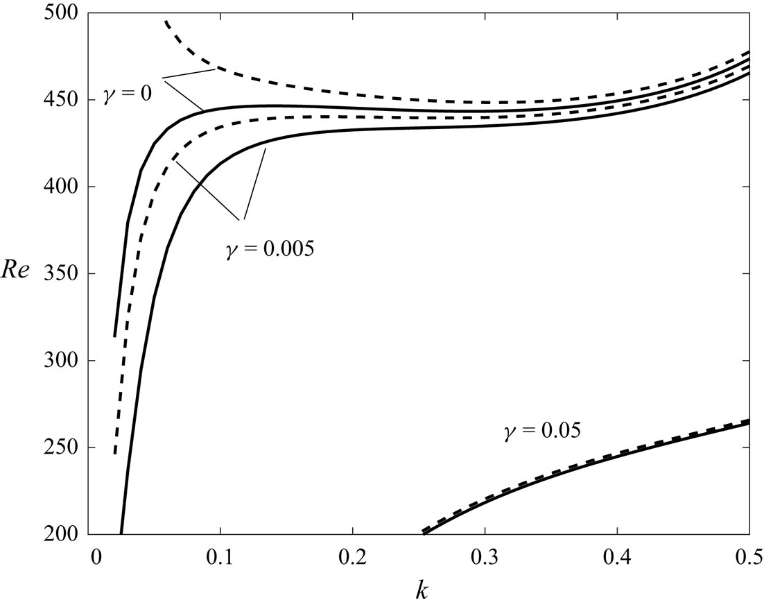This periodic regime corresponds to $\gamma =0$ and the transition from long wavelength instability to finite wavelength instability is achieved by varying the frequency parameter from $\beta =5.84$ to $\beta =5.85$, as can be seen in figures 8 and 14. Thereafter, it turns out that for $\omega ={1}/{\sqrt {37}}$ and for small amplitude ratios, $\gamma =0.005, \gamma =0.05$, there is suppression of the finite wavelength instability and only long wavelength instability exists.

Figure 14.

Marginal stability curves for different values of $\gamma$ with $\chi =0$ (absence of gravity), $\varPsi =0.05, \omega ={1}/{\sqrt {37}}$. The continuous lines correspond to $\beta =5.84$ and the broken lines correspond to $\beta =5.85$.

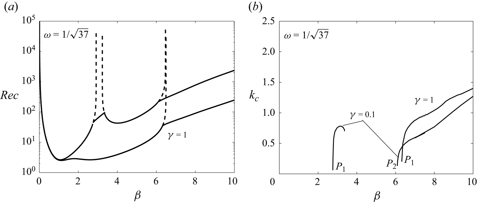
This time, we consider in figure 15 the case where gravity is present $\chi =1$, but still for $\omega ={1}/{\sqrt {37}}$. The evolution of the critical Reynolds number, ${Rec}$, and that of the critical wavenumber, $k_c$, as a function of the frequency parameter, $\beta$, are presented for two values of the velocity ratio. By introducing a weak quasi-periodicity in expression (2.8), figure 15(a) shows that for $\gamma =0.1$, there are two U-shaped zones in the intervals $0 \leq \beta \leq 2.91$ and $3.23 \leq \beta \leq 6. 47$ where the instability corresponds to long wavelengths. Moreover, in the middle of these two U-shaped curves and to the right of them, two oblique lines are associated with a finite wavelength instability and whose wavenumber evolutions are presented in figure 15(b). The finite wavelength instability in the middle is suppressed for $\gamma =1$ and the two unstable U-shaped curves merge into a single one in the interval $0 \leq \beta \leq 6.49$ where the critical Reynolds numbers are smaller (destabilizing effect). As for the last oblique line, i.e. $\beta >6$, it undergoes a translation towards lower Reynolds numbers. This destabilizing effect is accompanied by a shift in wavenumbers towards higher values, as shown in figure 15(b).

Figure 15.

Evolution of the critical Reynolds number and the critical wavenumber as a function of the frequency parameter, $\beta$, for $\gamma =0.1$ and $\gamma =1$ with $\chi =1, \varPsi =0.05$ and $\omega ={1}/{\sqrt {37}}$.

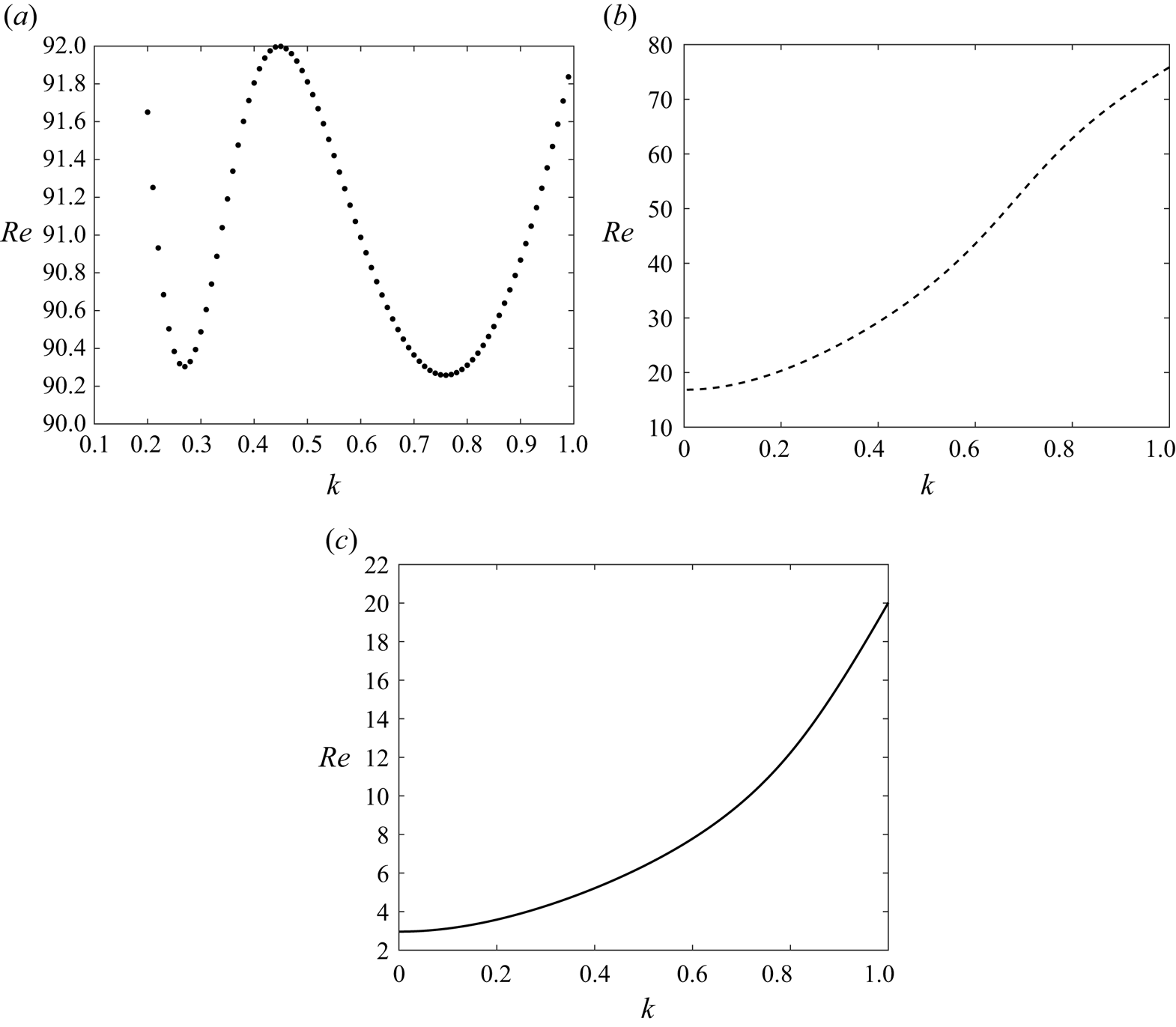
Finally, for small wavenumbers, figure 16 illustrates the influence of the amplitude ratio $\gamma$ on the marginal stability in the $(Re, k)$ plane. As can be seen, for $\gamma =0.1$, finite wavelength instability dominates. However, beyond $\gamma =0.1$, the threshold instability disappears and only the long wavelength instability becomes dominant.

Figure 16.

Transition from finite wavelength instability to long wavelength instability. Variation of the Reynolds number versus the wavenumber with $\chi =1 , \varPsi =0.05, \beta =3.3$ and $\omega ={1}/{\sqrt {37}}$, for different values of $\gamma$: $(\textit {a})\ \gamma =0.1, (\textit {b})\ \gamma =0.2$ and $(\textit {c})\ \gamma =1$.

7. Conclusion

In this study we examined the effect of quasi-periodic oscillation with two incommensurate frequencies of a horizontal wall, delimiting the bottom of a thin Newtonian fluid layer, on the stability of the base flow and the stability of the free surface. We first performed an asymptotic analysis for small wavenumbers, which enabled us to determine the function involved in the long wavelength instability criterion. We then showed that the maximum of this function depends strongly on frequency ratios. Furthermore, we found that the frequency ratio and its inverse have the same maximum, which occurs for two different values of the frequency parameter, which become spaced as the frequency ratio and its inverse become spaced. This scientific insight suggesting that the behaviour of the asymptotic function remains invariant when the frequency ratio is inverted provides this study with valuable implications for understanding the dynamic response of the system under various excitation conditions.

For arbitrary wavenumbers, we solved the quasi-periodic Orr–Sommerfeld equation derived from the conservation equations and associated with the interface and non-slip conditions at the horizontal wall, using Chebyshev's spectral collocation methods for spatial resolution and Floquet's theory by approximating the irrational frequency ratio by a rational number. Comparison between the asymptotic method used for long wavelengths and the numerical method showed good agreement between the results of the two methods.

On the one hand, numerical results showed that the neutral stability curves, Reynolds number versus wavenumber, depend strongly on the ratio of the two frequencies when the latter decreases from $\omega =\sqrt {37}$ to ${1}/{\sqrt {37}}$ for a fixed frequency parameter. This decreasing favours instability at long wavelengths and suppresses instability at finite wavelengths.

On the other hand, numerical results also showed that the alternation between non-threshold instabilities (long-wave U-shaped instability) and threshold instabilities (oblique curves) in the ($Rec, \beta$) plane is also altered by the frequency ratio. Indeed, decreasing this ratio from $\omega =\sqrt {37}$ to ${1}/{\sqrt {37}}$, suppresses the second and third U-shaped instabilities, as well as the second and third oblique curves (threshold instability), leading to a widening of the first U-shaped curve and the first oblique instability in the frequency ratio interval considered by Or (Reference Or1997) and Yih (Reference Yih1968), i.e. $0\leq \beta \leq 10$. This intriguing phenomenon of suppression indicates a distinct alteration in the stability behaviour of the system, where, for the same frequency ratios, there is also suppression of the corresponding branches of critical wavenumbers. This behaviour highlights the nuanced response of the system, where changes in frequency ratio contribute to varying degrees to the modification of stability diagrams.

Finally, the effect of the ratio of superimposed velocity amplitudes was also examined and it turns out that the increase of the amplitude makes it possible to pass, for example, from two instabilities in the shape of ${\rm U}$ towards only one occupying all the width of the interval of the frequency parameter of the two initial instabilities with a destabilizing effect. However, the increase of the amplitude ratio suppresses the instability of finite wavelength in the area of low values of the frequency parameter.

Acknowledgements

The authors would like to thank the unknown referees for their remarks and suggestions, which improved the work considerably.

Declaration of interest

The authors report no conflict of interest.

References

Blennerhassett, P.J. & Bassom, A.P. 2002 The linear stability of flat Stokes layers. J. Fluid Mech. 464, 393–410.CrossRef Google Scholar

Boulal, T., Aniss, S., Belhaq, M. & Azouani, A. 2008 Effect of quasi-periodic gravitational modulation on the convective instability in Hele-Shaw cell. Intl J. Non-Linear Mech. 43 (9), 852–857.CrossRef Google Scholar

Boulal, T., Aniss, S., Belhaq, M. & Rand, R. 2007 Effect of quasiperiodic gravitational modulation on the stability of a heated fluid layer. Phys. Rev. E 76 (5), 056320.CrossRef Google Scholar PubMed

Burya, A.G. & Shkadov, V.Y. 2001 Stability of a liquid film flowing down an oscillating inclined surface. Fluid Dyn. 36 (5), 671–681.CrossRef Google Scholar

Canuto, C., Hussaini, M.Y., Quarteroni, A. & Zang, T.A. 2007 Spectral Methods: Evolution to Complex Geometries and Applications to Fluid Dynamics. Springer Science & Business Media.CrossRef Google Scholar

Cowley, S.J. 1987 High frequency Rayleigh instability of Stokes layers. In Stability of Time Dependent and Spatially Varying Flows (ed. D.L. Dwoyer & M.Y. Hussaini), pp. 261–275. Springer.CrossRef Google Scholar

El Jaouahiry, A. & Aniss, S. 2020 Linear stability analysis of a liquid film down on an inclined plane under oscillation with normal and lateral components in the presence and absence of surfactant. Phys. Fluids 32 (3), 034105.CrossRef Google Scholar

Gao, P. & Lu, X.Y. 2008 Instability of an oscillatory fluid layer with insoluble surfactants. J. Fluid Mech. 595, 461–490.CrossRef Google Scholar

Garih, H., Strzelecki, A., Casalis, G. & Estivalezes, J.L. 2013 Detailed analysis of the vibration induced instability of a liquid film flow. Phys. Fluids 25 (1), 014101.CrossRef Google Scholar

Hall, P. 2003 On the instability of Stokes layers at high Reynolds numbers. J. Fluid Mech. 482, 1–15.CrossRef Google Scholar

Hall, P. & Stuart, J.T. 1975 The stability of Poiseuille flow modulated at high frequencies. Proc. R. Soc. Lond. A Math. Phys. Sci. 344 (1639), 453–464.Google Scholar

Hall, P. & Stuart, J.T. 1978 The linear stability of flat Stokes layers. Proc. R. Soc. Lond. A Math. Phys. Sci. 359 (1697), 151–166.Google Scholar

Isakova, K., Pralits, J.O., Repetto, R. & Romano, M.R. 2014 A model for the linear stability of the interface between aqueous humor and vitreous substitutes after vitreoretinal surgery. Phys. Fluids 26 (12), 124101.CrossRef Google Scholar

Kerczek, C.V. & Davis, S.H. 1974 Linear stability theory of oscillatory Stokes layers. J. Fluid Mech. 62 (4), 753–773.CrossRef Google Scholar

Khan, T. & Eslamian, M. 2019 Experimental analysis of one-dimensional Faraday waves on a liquid layer subjected to horizontal vibrations. Phys. Fluids 31 (8), 082106.CrossRef Google Scholar

Khan, T. & Eslamian, M. 2020 Experimental study on travelling and standing pattern formation and capillary waves in a pinned liquid film: effects of multi-axis lateral (horizontal) vibrations and substrate geometry. J. Fluid Mech. 900, A30.CrossRef Google Scholar

Lin, S.P., Chen, J.N. & Woods, D.R. 1996 Suppression of instability in a liquid film flow. Phys. Fluids 8 (12), 3247–3252.CrossRef Google Scholar

Meskauskas, J., Repetto, R. & Siggers, J.H. 2011 Oscillatory motion of a viscoelastic fluid within a spherical cavity. J. Fluid Mech. 685, 1–22.CrossRef Google Scholar

Nayfeh, A.H. & Mook, D.T. 2008 Nonlinear Oscillations. John Wiley & Sons.Google Scholar

Or, A.C. 1997 Finite-wavelength instability in a horizontal liquid layer on an oscillating plane. J. Fluid Mech. 335, 213–232.CrossRef Google Scholar

Salwen, H. & Grosch, C.E. 1972 The stability of Poiseuille flow in a pipe of circular cross-section. J. Fluid Mech. 54 (1), 93–112.CrossRef Google Scholar

Samanta, A. 2017 Linear stability of a viscoelastic liquid flow on an oscillating plane. J. Fluid Mech. 822, 170–185.CrossRef Google Scholar

Samanta, A. 2019 Effect of electric field on an oscillatory film flow. Phys. Fluids 31 (3), 034109.CrossRef Google Scholar

Samanta, A. 2021 Instability of a shear-imposed flow down a vibrating inclined plane. J. Fluid Mech. 915, A93.CrossRef Google Scholar

Straatman, A.G., Khayat, R.E., Haj-Qasem, E. & Steinman, D.A. 2002 On the hydrodynamic stability of pulsatile flow in a plane channel. Phys. Fluids 14 (6), 1938–1944.CrossRef Google Scholar

Talib, E. & Juel, A. 2007 Instability of a viscous interface under horizontal oscillation. Phys. Fluids 19 (9), 092102.CrossRef Google Scholar

Thomas, C. 2020 The linear stability of an acceleration-skewed oscillatory Stokes layer. J. Fluid Mech. 895, A27.CrossRef Google Scholar

Tim, D., Steve, S., Tim, D. & Teifi, J. 1998 A model for the fluid motion of vitreous humour of the human eye during saccadic movement. Phys. Med. Biol. 43, 1385.Google Scholar

Trefethen, L.N. 2000 Spectral Methods in MATLAB. Society for Industrial and Applied Mathematics.CrossRef Google Scholar

Von Kerczek, C.H. 1982 The instability of oscillatory plane Poiseuille flow. J. Fluid Mech. 116, 91–114.CrossRef Google Scholar

Weideman, J.A. & Reddy, S.C. 2000 A MATLAB differentiation matrix suite. ACM Trans. Math. Softw. 26 (4), 465–519.CrossRef Google Scholar

Woods, D.R. & Lin, S.P. 1995 Instability of a liquid film flow over a vibrating inclined plane. J. Fluid Mech. 294, 391–407.CrossRef Google Scholar

Yagoubi, M. & Aniss, S. 2017 Effect of vertical quasi-periodic vibrations on the stability of the free surface of a fluid layer. Eur. Phys. J. Plus 132 (5), 1–13.CrossRef Google Scholar

Yih, C.S. 1968 Instability of unsteady flows or configurations part 1. Instability of a horizontal liquid layer on an oscillating plane. J. Fluid Mech. 31 (4), 737–751.CrossRef Google Scholar

Yuan, J. & Wang, D. 2019 An experimental investigation of acceleration-skewed oscillatory flow over vortex ripples. J. Geophys. Res.: Oceans 124 (12), 9620–9643.CrossRef Google Scholar

Figure 1.Newtonian fluid layer on an oscillating horizontal wall.

Figure 2.Time evolution of base velocity profiles for $\beta =3, \gamma =1$ and different frequency ratios over the time interval $[0,{\rm \pi} ]$.

Figure 3.Time evolution of base velocity profiles for $\beta =10, \gamma =1$ and different frequency ratios over the time interval $[0,{\rm \pi} ]$.

Figure 4.Time evolution of the base velocity profile for $\gamma =1, \beta = 3$ and for different locations: $y=-0.25,-0.5, -0.75,-1$.

Figure 5.Variation of the function $10 \times F(\beta )$, defined by expression (3.24), as a function of $\beta$, (a) for different values of $\gamma$, with $\omega =\sqrt 37$ and (b) for different values of $\omega$, with $\gamma =1$.

Table 1.The maximum of the evolution of the analytical function $10\times F(\beta )$ when $\gamma =1, \chi =1$ and $\varPsi = 0.05$.

Figure 6.Convergence of the growth rate $\lambda _r$ as a function of the number of Chebychev collocation points $N$ for the cases (a) $\beta =3, Re=100$ and (b) $\beta =8, Re=5000$, with $\omega =\sqrt {37}, \chi =1 , \varPsi =0.05$ and $\gamma =1$.

Figure 7.Comparison of asymptotic and numerical growth rates for (a) $\omega =\sqrt {37}$ and (b) $\omega =1/\sqrt {37}$ for $\beta =2, Re=50, \chi =1, \varPsi = 0.05$ and $\gamma =0$.

Table 2.Comparison between analytical results at long wavelengths and numerical results with $\omega ={\omega _2}/{\omega _2}=1, \chi =1$ and $\varPsi = 0.05$.

Figure 8.Marginal stability curves for $\chi =0, \varPsi =0.05$ and $\gamma =0$. Instability without threshold (long wavelength) for $\beta =5.84$ and with threshold (finite wavelength) for $\beta =5.85$.

Figure 9.Effect of the frequency ratio, $\omega$, on marginal stability curves for $\chi =1 , \varPsi =0.05, \beta =3.5$ and $\gamma =1$, (a) $\omega =\sqrt {37}$, (b) $\omega =\sqrt {7}$, (c) $\omega =\sqrt {2}$, (d) $\omega =1/\sqrt {2}$, (e) $\omega =1/\sqrt {7}$ and (f) $\omega =1/\sqrt {37}$.

Figure 10.Marginal stability curves corresponding to the branch points for $\chi =1 , \varPsi =0.05$ and $\gamma =1$.

Figure 11.Growth rate $\lambda _r$ versus the wavenumber $k$ for $\chi =1 , \varPsi =0.05$ and $\gamma =1$. Here $\beta =2.56$ corresponds to long wavelength instability and $\beta =2.57$ corresponds to finite wavelength instability.

Figure 12.Effect of the irrational frequency ratio on the stability diagram in the $(Rec, \beta )$ plane. Evolution of the critical Reynolds number $Rec$ versus the frequency parameter $\beta$ for several frequency ratios, $\omega$, and for $\chi =1, \varPsi =0.05$ and $\gamma =1$. The boundaries of long wavelengths are denoted by the vertical dotted lines, the boundaries of finite wavelengths are denoted by the oblique lines. The solid lines represent the variation of the critical Reynolds number $Rec$, while the dashed lines do not represent a criticality because of the domination of long wavelengths.

Table 3.Effect of the frequency ratio, $\omega$, on the branch points $P1, P2$ and $P3$, with $\gamma =1, \chi =1$ and $\varPsi =0.05$.

Figure 13.Variation of the wavenumber $k _{c}$ (finite wavelength instability) as a function of the parameter $\beta$, for $\chi =1 , \varPsi =0.05$ and $\gamma =1$.

Figure 14.Marginal stability curves for different values of $\gamma$ with $\chi =0$ (absence of gravity), $\varPsi =0.05, \omega ={1}/{\sqrt {37}}$. The continuous lines correspond to $\beta =5.84$ and the broken lines correspond to $\beta =5.85$.

Figure 15.Evolution of the critical Reynolds number and the critical wavenumber as a function of the frequency parameter, $\beta$, for $\gamma =0.1$ and $\gamma =1$ with $\chi =1, \varPsi =0.05$ and $\omega ={1}/{\sqrt {37}}$.

Figure 16.Transition from finite wavelength instability to long wavelength instability. Variation of the Reynolds number versus the wavenumber with $\chi =1 , \varPsi =0.05, \beta =3.3$ and $\omega ={1}/{\sqrt {37}}$, for different values of $\gamma$: $(\textit {a})\ \gamma =0.1, (\textit {b})\ \gamma =0.2$ and $(\textit {c})\ \gamma =1$.

Article contents

Linear stability analysis of a thin liquid film on a horizontal wall under quasi-periodic oscillation

Abstract

JFM classification

Information

1. Introduction

2. Mathematical formulation

2.1. Governing equations

2.2. Base flow

2.3. Stability and normal modes analysis

3. Asymptotic solution in the long wavelength limit

3.0.1. Order $k^0$:

3.0.2. Order $k^1$:

3.0.3. Order $k^2$:

4. Numerical procedure for arbitrary wavenumber

4.1. Spatial discretization

4.2. Floquet analysis

5. Validation of the numerical procedure

6. Results and discussion

6.1. Influence of the frequency ratio, $\omega ={\omega _2}/{\omega _1}$, on the marginal stability curves: $(Re,k)$

6.2. Influence of the frequency ratio, $\omega ={\omega _2}/{\omega _1}$, on the instability threshold in the plane ($Re_c,\beta$) and ($k_c,\beta$)

6.2.1. Stability diagram in the plane $(Rec, \beta )$

6.2.2. Stability diagram in the plane $(k_c, \beta )$

6.3. Effect of the ratio of superimposed velocity amplitudes

7. Conclusion

Acknowledgements

Declaration of interest

References

Save article to Kindle

Save article to Dropbox

Save article to Google Drive

Reply to: Submit a response

Your details

You have entered the maximum number of contributors

Conflicting interests