1 Introduction
Collective motion is ubiquitous in the biological and natural systems. When the collections of bodies move in a fluid, the motion of each is influenced by others through the flow-mediated interactions among them. The collective fluid–structure interactions, leading to the complex flow and the motion of individuals, may be further categorized into two subsets: passively moving bodies and actively moving bodies in a fluid. Typical flow problems for the former category are sedimentations of particles and fibres (Guazzelli & Hinch Reference Guazzelli and Hinch2011), in which bodies passively respond to external forcing. On the other hand, for the latter category the interactions among actively moving bodies in a fluid are more complicated. The previous studies have largely focused on the low Reynolds number collective systems, such as swimming micro-organisms and micro-particles (e.g. Saintillan & Shelley Reference Saintillan and Shelley2008; Zhang et al.
Reference Zhang, Beer, Florin and Swinney2010; Peruani et al.
Reference Peruani, Starruss, Jakovljevic, Søgaard-Andersen, Deutsch and Bär2012). The most fascinating examples for higher Reynolds number collective systems are bird flocks and fish schools, in which both structure and behaviour are similar (Major & Dill Reference Major and Dill1978). The individuals derive many benefits from the collective behaviour in many perspectives such as foraging, reproduction and defence from predators (Partridge Reference Partridge1982; Parrish & Edelstein-Keshet Reference Parrish and Edelstein-Keshet1999; Sumpter Reference Sumpter2006; Bajec & Heppner Reference Bajec and Heppner2009). It is also plausible that the individuals in group save on the energetic cost of locomotion through the flow-mediated interactions in view of hydrodynamics. For example, the
 $V$
formation maybe improves efficiency of flying birds by favourable interactions with the up- and down-wash of leading neighbours, particularly over long migratory routes (Lissaman & Shollenberger Reference Lissaman and Shollenberger1970; Hummel Reference Hummel1983). Similarly, fish in schools are supposed to obtain a hydrodynamic advantage, thus reducing the cost of locomotion, by taking advantage of the wakes shed by neighbours within the school (Weihs Reference Weihs1973, Reference Weihs1975; Hemelrijk et al.
Reference Hemelrijk, Reid, Hildenbrandt and Padding2015).
Although the invaluable insight into the social traits of collective locomotion, such as schooling and flocking, has been provided by investigations based on experiments and models (Couzin et al. Reference Couzin, Krause, James, Ruxton and Franks2002, Reference Couzin, Krause, Franks and Levin2005; Viscido, Parrish & Grünbaum Reference Viscido, Parrish and Grünbaum2005), several issues about the role of hydrodynamics in collective locomotion are still open questions (Weihs Reference Weihs1973; Partridge & Pitcher Reference Partridge and Pitcher1979; Daghooghi & Borazjani Reference Daghooghi and Borazjani2015). One important and intriguing issue is the hydrodynamic advantage. The theoretical research on this issue was firstly conducted by Weihs (Reference Weihs1973, Reference Weihs1975), who suggested that schooling fish could greatly enhance their thrust production in a diamond configuration using an inviscid potential flow model. Moreover, the swimmer could hydrodynamically gain benefit from its neighbours due to two physical mechanisms: vortex hypothesis and channelling effect (Weihs Reference Weihs1975; Dong & Lu Reference Dong and Lu2007; Daghooghi & Borazjani Reference Daghooghi and Borazjani2015). However, little biological evidence of hydrodynamic advantage in the diamond pattern has been found (Partridge & Pitcher Reference Partridge and Pitcher1979). Abrahams & Colgan (Reference Abrahams and Colgan1987) pointed out the controversy may be derived from ignoring the potential trade-offs involved in school functions. Due to the difficulty of experimental measurement on the energetic savings of schooling and flocking, only limited experimental evidence (Killen et al. Reference Killen, Marras, Steffensen and McKenzie2012; Portugal et al. Reference Portugal, Hubel, Fritz, Heese, Trobe, Voelkl, Hailes, Wilson and Usherwood2014; Ashraf et al. Reference Ashraf, Bradshaw, Ha, Halloy, Godoy-Diana and Thiria2017) has showed that the individuals can obtain an aero- or hydrodynamic advantage from the collective locomotion. The other issue is the role of flows on the emergence of the collective pattern. To investigate this issue, individuals may be modelled as vortex dipoles (Gazzola et al. Reference Gazzola, Tchieu, Alexeev, de Brauer and Koumoutsakos2016). In addition, if swimmers are able to optimize their motions in response to nonlinearly varying hydrodynamic loads, a stable geometrical formation can be maintained (Gazzola et al. Reference Gazzola, Tchieu, Alexeev, de Brauer and Koumoutsakos2016). However, the hydrodynamics is not fully resolved in the model of vortex dipoles. To assess the role of aero- or hydrodynamics in collective swimming and flying, more quantitative information is needed.
As the simplest model of the basic element for schooling and flocking, the grouping unit, consisting of two individuals in a tandem or side-by-side configuration in uniform flow, has been studied by experiments and simulations. This approach provided a promising means toward better understanding the basic principle how aero- or hydrodynamic coupling between closely packed neighbours influences propulsive performance. Dong & Lu (Reference Dong and Lu2007) have numerically investigated the flow over travelling wavy foils in a side-by-side arrangement. It is revealed that the lateral interference is of benefit to saving the swimming power in the in-phase case and enhancing the forces in the antiphase case. More recently, Dewey et al. (Reference Dewey, Quinn, Boschitsch and Smits2014) and Boschitsch, Dewey & Smits (Reference Boschitsch, Dewey and Smits2014) have presented their experimental results on the propulsive performance of two identical bio-inspired hydrofoils arranged in side-by-side and in-line configuration as they undergo prescribed pitching motions over a wide range of phase lags and spacings between the foils. It is found that when the foils are arranged in a side-by-side configuration, their propulsive efficiencies are enhanced at the cost of a reduction in thrust for in-phase oscillations, which is consistent with the observations by Dong & Lu (Reference Dong and Lu2007); while for antiphase oscillations, each foil’s thrust is enhanced and the propulsive efficiency almost remains unchanged. When the foils are arranged in an in-line configuration (Boschitsch et al. Reference Boschitsch, Dewey and Smits2014), the thrust production and propulsive efficiency of the upstream foil differs from those of an isolated one only for relatively closely spaced foils. In contrast, the performance of the downstream foil depends strongly on the streamwise spacing and phase differential between the foils. Similar studies on the performance of two flapping foils have also been conducted (Warkentin & DeLaurier Reference Warkentin and DeLaurier2007; Broering, Lian & Henshaw Reference Broering, Lian and Henshaw2012).
However, in the studies above, the swimmers were held fixed in an oncoming flow and could not propel themselves freely. The collective configuration of swimmers is predefined and not affected by the hydrodynamic interactions between them. On the other hand, the self-propelled swimmers or flyers in collective locomotion are free to select their speed and relative position through flow-mediated interactions among them. It is essential to capture this trait in order to understand the role of aero- or hydrodynamic interactions on the emergence of a collective pattern.
Recent studies turn their attention to the emergence of collective locomotion dynamics in a two-body self-propelled system. Becker et al. (Reference Becker, Masoud, Newbolt, Shelley and Ristroph2015) studied experimentally the flapping wings swimming in rotational orbits to mimic an infinite array of locomotors in which the inter-wing spacing is fixed. The self-propelled wings choose one of fast and slow modes which correspond to constructive and destructive wing–wake interactions. Inspired by Becker et al. (Reference Becker, Masoud, Newbolt, Shelley and Ristroph2015), Ramananarivo et al. (Reference Ramananarivo, Fang, Oza, Zhang and Ristroph2016) further carried out an experiment based on a similar system composed of tandem wings flapping in synchrony. The difference is that inter-wing spacing is no longer fixed but dynamically selected as a result of flow-mediated coupling between the wings. Thus it is possible to understand the emergent locomotion dynamics and assess the role of flow-mediated interactions in the collective locomotion. The experiment showed that multiple stable configurations of tandem swimmers can emerge spontaneously, which offers experimental support for the Lighthill conjecture (Lighthill Reference Lighthill1975; Ramananarivo et al. Reference Ramananarivo, Fang, Oza, Zhang and Ristroph2016).
Compared with the experimental studies, numerical simulations can provide more quantitative information, especially regarding thrust and power, which are crucial to investigate collective advantages such as energetic savings and performance enhancement. A single flexible flapping plate moving freely in a stationary fluid was used as a model of self-propulsion for swimming and flying in previous studies (Hua, Zhu & Lu Reference Hua, Zhu and Lu2013; Zhu, He & Zhang Reference Zhu, He and Zhang2014b
). However, few numerical investigations are performed that focus on the flow-mediated interactions among two or more self-propelled bodies. As far as we know, the only study was conducted by Zhu, He & Zhang (Reference Zhu, He and Zhang2014a
). Their two self-propelled flapping filaments in a tandem configuration showed that multiple stable configurations can be spontaneously formed with the help of the vortex street behind the leader. The follower can enjoy energetic benefits for the cases with
 $2S$
wakes. The energetic advantage of the leader was found in the compact in-line configuration, but not the loose in-line configuration. Zhu et al. (Reference Zhu, He and Zhang2014a
) mainly considered the long-range interaction in a tandem pair of swimmers. The flow picture seems to be analogous to that of a swimmer in vortex-street wakes (Alben Reference Alben2010).
These experimental and numerical results above show that flow-mediated interactions alone are sufficient to generate tandem formation and lead to collective advantages, which reflect the longitudinal influence of the flows between the leader and the follower. Our study differs from previous studies in several important ways. First and foremost, we take a step toward seeking the possibilities of more general stable configurations by introducing lateral spacing between two bodies, and examining its influence. Second, we mainly focus on the tight and compact configurations in which the short-range flow interaction instead of the long-range interaction (Zhu et al. Reference Zhu, He and Zhang2014a ; Becker et al. Reference Becker, Masoud, Newbolt, Shelley and Ristroph2015; Ramananarivo et al. Reference Ramananarivo, Fang, Oza, Zhang and Ristroph2016) dominates the collective dynamics. It should be noted that the compact configurations have been proven to be remarkably common and representative in natural schools and flocks by the experimental measurements (Graves Reference Graves1977; Major & Dill Reference Major and Dill1978; Partridge & Pitcher Reference Partridge and Pitcher1979; Partridge et al. Reference Partridge, Pitcher, Cullen and Wilson1980; Ashraf et al. Reference Ashraf, Godoy-Diana, Halloy, Collignon and Thiria2016, Reference Ashraf, Bradshaw, Ha, Halloy, Godoy-Diana and Thiria2017). Specifically, we consider a grouping unit consisting of two flexible plates placed in an initial side-by-side configuration with the lateral and longitudinal spacings. The self-propulsion is induced by the prescribed heave motion at the leading edge of each plate but whose longitudinal swimming is free. Due to fluid mediation, several stable configurations are expected to form. Corresponding propulsive properties, unsteady dynamics and flow structures around the plates are systematically investigated.
The remainder of this paper is organized as follows. The physical problem and mathematical formulation are presented in § 2. The numerical method and validation are described in § 3. Detailed results are discussed in § 4 and concluding remarks are addressed in § 5.
2 Physical problem and mathematical formulation
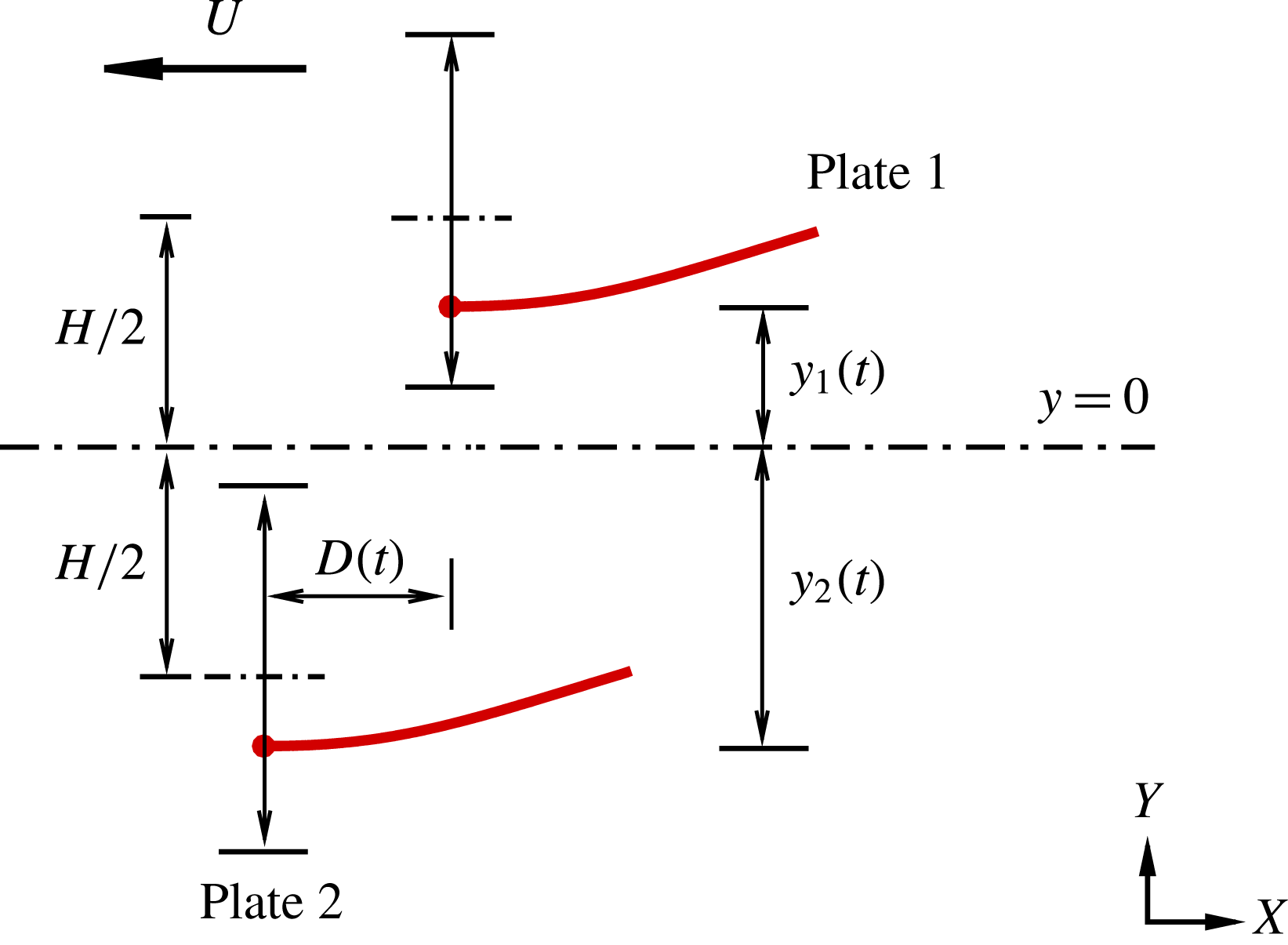
Sketch of a model for the collective locomotion of two flapping plates which are initially placed in a side-by-side configuration. The lateral and longitudinal distances between them are
 $H$
and
 $D$
, respectively. They have been normalized by the dimensional length of the plate
 $L$
. When the leading edges are forced to heave vertically and sinusoidally, the plates deform passively and move in the horizontal direction freely. Here
 $y_{i}(t)$
(
 $i=1$
or
 $2$
) denotes the lateral position of the leading edge of plate
 $i$
, and
 $y_{1}=H/2$
and
 $y_{2}=-H/2$
are the equilibrium positions of the leading edges.

As shown in figure 1, two plates are placed initially in a side-by-side configuration. The plates are immersed in a stationary viscous incompressible fluid. The leading edges of the two plates are forced to heave sinusoidally with identical amplitude
 $A$
and frequency
 $f$
in the lateral direction. The forced motions of the leading edges are prescribed by
 $$\begin{eqnarray}\displaystyle & \displaystyle y_{1}(t)=A\cos (2\unicode[STIX]{x03C0}ft)+H/2, & \displaystyle\end{eqnarray}$$
 $$\begin{eqnarray}\displaystyle & \displaystyle y_{2}(t)=A\cos (2\unicode[STIX]{x03C0}ft+\unicode[STIX]{x1D719})-H/2, & \displaystyle\end{eqnarray}$$
where the subscripts 1 and 2 denote the upper and lower plate, respectively;
 $H$
is the lateral spacing between the equilibrium positions of the two plates, which is fixed in all simulations; and
 $\unicode[STIX]{x1D719}$
is the phase difference between the flapping plates. Here, two typical phase differences
 $\unicode[STIX]{x1D719}=0$
and
 $\unicode[STIX]{x03C0}$
are considered which can be described as the in-phase and antiphase scenarios, respectively. In addition, the plates are unconstrained in the horizontal direction and thus the longitudinal spacing
 $D(t)$
is dynamically selected as a result of flow-mediated coupling between the two plates. In all simulations, if not specified, usually the initial longitudinal distance
 $D_{0}=D(t=0)=0$
. The active pitching angle is zero in this model which means that only the leading edges of the plates are restricted with the prescribed vertical motion and the remainder of each plate can move freely in the entire fluid domain.
To investigate the system of the fluid flow and the flapping plates, the incompressible Navier–Stokes equations are used to simulate the fluid flow,
 $$\begin{eqnarray}\displaystyle & \displaystyle \frac{\unicode[STIX]{x2202}\boldsymbol{v}}{\unicode[STIX]{x2202}t}+\boldsymbol{v}\boldsymbol{\cdot }\unicode[STIX]{x1D735}\boldsymbol{v}=-\frac{1}{\unicode[STIX]{x1D70C}}\unicode[STIX]{x1D735}p+\frac{\unicode[STIX]{x1D707}}{\unicode[STIX]{x1D70C}}\unicode[STIX]{x1D6FB}^{2}\boldsymbol{v}+\boldsymbol{f}_{b}, & \displaystyle\end{eqnarray}$$
 $$\begin{eqnarray}\displaystyle & \displaystyle \unicode[STIX]{x1D735}\boldsymbol{\cdot }\boldsymbol{v}=0, & \displaystyle\end{eqnarray}$$
where
 $\boldsymbol{v}$
is the velocity,
 $p$
the pressure,
 $\unicode[STIX]{x1D70C}$
the density of the fluid,
 $\unicode[STIX]{x1D707}$
the dynamic viscosity and
 $\boldsymbol{f}_{b}$
the Eulerian momentum force acting on the surrounding fluid due to the immersed boundary, as constrained by the no-slip boundary condition.
The structural equation is employed to describe the deformation and motion of the plates (Connell & Yue Reference Connell and Yue2007; Hua et al. Reference Hua, Zhu and Lu2013),
 $$\begin{eqnarray}\displaystyle \unicode[STIX]{x1D70C}_{l}\frac{\unicode[STIX]{x2202}^{2}\boldsymbol{X}}{\unicode[STIX]{x2202}t^{2}}-\frac{\unicode[STIX]{x2202}}{\unicode[STIX]{x2202}s}\left[Eh\left(1-\left|\frac{\unicode[STIX]{x2202}\boldsymbol{X}}{\unicode[STIX]{x2202}s}\right|^{-1}\right)\frac{\unicode[STIX]{x2202}\boldsymbol{X}}{\unicode[STIX]{x2202}s}\right]+EI\frac{\unicode[STIX]{x2202}^{4}\boldsymbol{X}}{\unicode[STIX]{x2202}^{4}s}=\boldsymbol{F}_{s}, & & \displaystyle\end{eqnarray}$$
where
 $s$
is the Lagrangian coordinate along the plate,
 $\boldsymbol{X}(s,t)=(X(s,t),Y(s,t))$
is the position vector of the plates,
 $\boldsymbol{F}_{s}$
is the Lagrangian force exerted on the plates by the surrounding fluid,
 $\unicode[STIX]{x1D70C}_{l}$
is the structural linear mass density.
 $Eh$
and
 $EI$
denote the structural stretching rigidity and bending rigidity, respectively. At the leading edges of the plates, the clamped boundary condition are adopted, i.e.
 $$\begin{eqnarray}\displaystyle -Eh\left(1-\left|\frac{\unicode[STIX]{x2202}\boldsymbol{X}}{\unicode[STIX]{x2202}s}\right|^{-1}\right)\frac{\unicode[STIX]{x2202}X}{\unicode[STIX]{x2202}s}+EI\frac{\unicode[STIX]{x2202}^{3}X}{\unicode[STIX]{x2202}^{3}s}=0,\quad Y(t)=y(t),\quad \frac{\unicode[STIX]{x2202}\boldsymbol{X}}{\unicode[STIX]{x2202}s}=(1,0).\qquad & & \displaystyle\end{eqnarray}$$
At the free ends of the plates, the boundary conditions are expressed as
 $$\begin{eqnarray}\displaystyle -Eh\left(1-\left|\frac{\unicode[STIX]{x2202}\boldsymbol{X}}{\unicode[STIX]{x2202}s}\right|^{-1}\right)\frac{\unicode[STIX]{x2202}\boldsymbol{X}}{\unicode[STIX]{x2202}s}+EI\frac{\unicode[STIX]{x2202}^{3}\boldsymbol{X}}{\unicode[STIX]{x2202}^{3}s}=0,\quad \frac{\unicode[STIX]{x2202}^{2}\boldsymbol{X}}{\unicode[STIX]{x2202}s^{2}}=0. & & \displaystyle\end{eqnarray}$$
Moreover,
 $\boldsymbol{X}(s,0)=(s,y_{i}(0)),\unicode[STIX]{x2202}\boldsymbol{X}/\unicode[STIX]{x2202}t(s,0)=(0,0)$
is the initial condition for plate
 $i$
.
The characteristic quantities
 $\unicode[STIX]{x1D70C}$
,
 $L$
and
 $U_{ref}$
are chosen to normalize the above equations. Here
 $L$
is the dimensional length of the plates,
 $U_{ref}$
is the maximum flapping velocity of the plunging motion, i.e.
 $U_{ref}=2\unicode[STIX]{x03C0}Af$
. Here, the characteristic time is
 $T_{ref}=L/U_{ref}$
. The dimensionless governing parameters are described as follows: the heaving amplitude
 $A$
, the Reynolds number
 $Re=\unicode[STIX]{x1D70C}U_{ref}L/\unicode[STIX]{x1D707}$
, the stretching stiffness
 $S=Eh/\unicode[STIX]{x1D70C}U_{ref}^{2}L$
, the bending stiffness
 $K=EI/\unicode[STIX]{x1D70C}U_{ref}^{2}L^{3}$
, the mass ratio of the plates and the fluid
 $M=\unicode[STIX]{x1D70C}_{l}/\unicode[STIX]{x1D70C}L$
, the phase difference
 $\unicode[STIX]{x1D719}$
, the lateral spacing
 $H$
and the initial longitudinal spacing
 $D_{0}$
.
3 Numerical method and validation
The governing equations of the fluid–plates problem are solved numerically by the lattice Boltzmann method (LBM) for the fluid flow and a finite element method for the deformation of the flexible plates. The immersed boundary (IB) method is applied to treat flow–structure interaction (Peskin Reference Peskin2002; Mittal & Iaccarino Reference Mittal and Iaccarino2005). The body force term
 $\boldsymbol{f}_{b}$
in (2.3) represents an interaction force between the fluid and the immersed boundary to enforce the no-slip velocity boundary condition. The lattice Boltzmann equation with the body force model (Chen & Doolen Reference Chen and Doolen1998) is employed to solve the viscous fluid flow. Equation (2.5) for the plate is discretized by a finite element method and deformations with a large displacement of the plate are handled by the corotational scheme (Doyle Reference Doyle2001). A detailed description of the numerical method can be found in our previous papers (Hua et al.
Reference Hua, Zhu and Lu2013; Hua, Zhu & Lu Reference Hua, Zhu and Lu2014).
Based on our convergence studies with different computational domains, the computational domain for fluid flow is chosen as
 $[-20,30]\times [-20,20]$
in the
 $x$
and
 $y$
directions, which is large enough so that the blocking effects of the boundaries are not significant. Following the scheme in Zou & He (Reference Zou and He1997), a constant pressure with
 $\boldsymbol{v}=0$
is imposed at all boundaries except for the outlet.
 $\unicode[STIX]{x2202}\boldsymbol{v}/\unicode[STIX]{x2202}x=0$
with constant pressure is imposed in the outlet (Zou & He Reference Zou and He1997). At the initial time, the fluid velocity field is zero in the entire computational domain. In the
 $x$
and
 $y$
directions the mesh is uniform with spacing
 $\unicode[STIX]{x0394}x=\unicode[STIX]{x0394}y=0.01L$
. The time step is
 $\unicode[STIX]{x0394}t=T/10\,000$
for the simulations of fluid flow and plate deformation, with
 $T=1/f$
being the flapping period. Moreover, a finite moving computational domain (Hua et al.
Reference Hua, Zhu and Lu2013) is used in the
 $x$
direction to allow the plates to move for a sufficiently long time. As the plate travel one lattice in the
 $x$
direction, the computational domain is shifted, i.e. one layer being added at the inlet and another layer being removed at the outlet (Hua et al.
Reference Hua, Zhu and Lu2013).
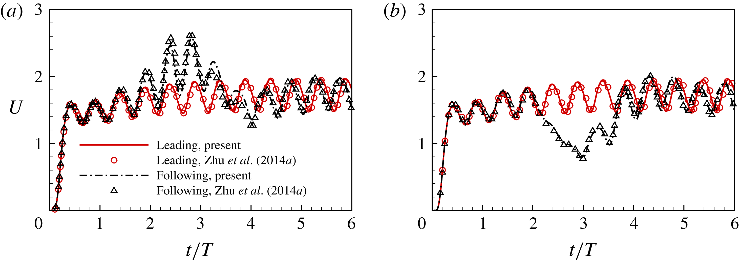
Validation for the case of two self-propelled plates in a tandem configuration with the dimensionless governing parameters
 $Re=200$
,
 $H=0$
,
 $A=0.5$
,
 $M=0.2$
,
 $K=0.8$
,
 $S=1000$
and
 $\unicode[STIX]{x1D719}=0$
. (a)
 $D_{0}=8.0$
and (b)
 $D_{0}=9.0$
(Zhu et al.
Reference Zhu, He and Zhang2014a
).

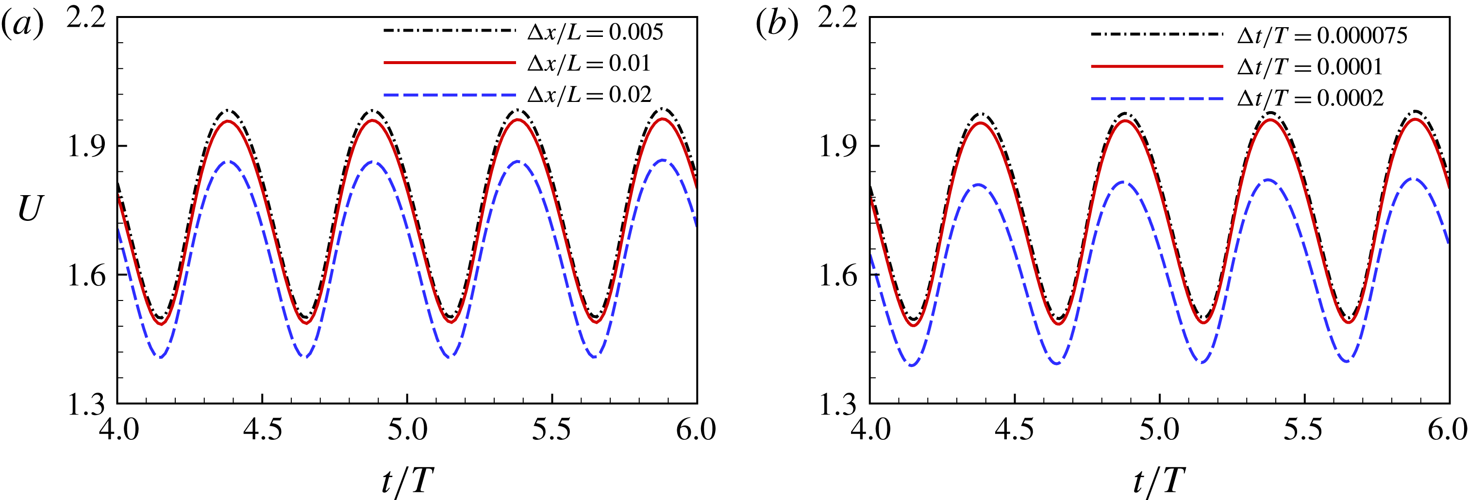
The grid independence (a) and time step independence (b) studies for the case with
 $M=0.2$
,
 $A=0.5$
,
 $D_{0}=9.0$
,
 $H=0$
,
 $K=0.8$
,
 $S=1000$
,
 $Re=200$
and
 $\unicode[STIX]{x1D719}=0$
. The streamwise velocities of the leading edges as a function of time are presented.

To validate the present numerical method, two cases with different initial distances for two self-propelled plates in a tandem configuration are simulated. Figure 2 shows the time-dependent streamwise velocity of the leading edge in two cases. It is seen that the present results agree well with those of Zhu et al. (Reference Zhu, He and Zhang2014a ).
The grid independence and time step independence studies were also performed. The results are shown in figure 3. It is seen that
 $\unicode[STIX]{x0394}x/L=0.01$
and
 $\unicode[STIX]{x0394}t/T=0.0001$
are sufficient to achieve accurate results. Hence, in all of our simulations,
 $\unicode[STIX]{x0394}x/L=0.01$
and
 $\unicode[STIX]{x0394}t/T=0.0001$
were adopted.
In addition, the numerical strategy used in this study has been validated and successfully applied to a wide range of flows, such as the dynamics of fluid flow over a circular flexible plate (Hua et al. Reference Hua, Zhu and Lu2014), the locomotion of a flapping flexible plate (Hua et al. Reference Hua, Zhu and Lu2013) and the vorticity dynamics of fluid flow over a flapping plate (Li & Lu Reference Li and Lu2012).
4 Results and discussion
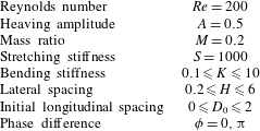
The parameters in the simulations.

We here present some typical results on the collective behaviours of two flapping plates due to the flow-mediated interactions. The settings of all governing parameters are shown in table 1. It is seen that
 $Re$
,
 $A$
,
 $M$
and
 $S$
are fixed in our simulation but the following four parameters are variable: the lateral spacing
 $(H)$
, the initial longitudinal spacing
 $(D_{0})$
, the bending stiffness
 $(K)$
and the phase difference
 $(\unicode[STIX]{x1D719})$
. In addition, the propulsive behaviours of an isolated plate are also simulated for comparison. The results of in-phase cases are presented in §§ 4.1–4.5. The results of antiphase cases are presented in § 4.6.
4.1 Emergent dynamics and configurations
In our numerical settings, the in-phase flapping scenario (
 $\unicode[STIX]{x1D719}=0$
) was first investigated. The bending stiffness
 $K=1$
is chosen at first because it lies in the optimal range of stiffness for the largest propulsive speed for the isolated plate. The side-by-side initial configurations with
 $D_{0}=0$
and
 $H\in (0.2,6)$
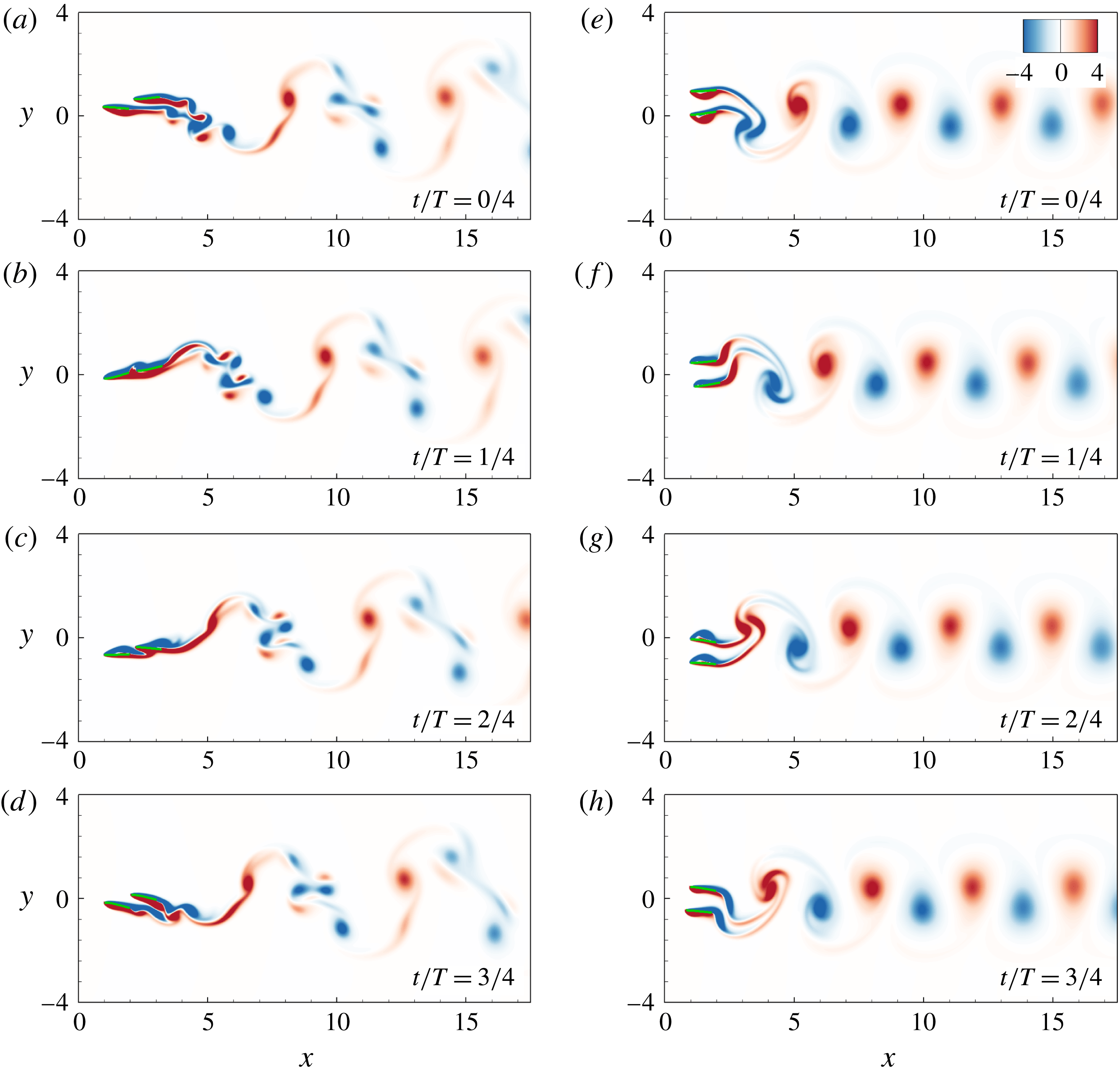
are examined. Four typical states of collective pattern are identified. They are formed spontaneously by the two-plate system, i.e. the staggered-following (SF) mode, alternate-leading (AL) mode, non-periodic (NP) mode and non-interfering (NI) mode.
Instantaneous vorticity contours at
 $t=(0/4)T$
,
 $T/4$
,
 $T/2$
and
 $(3/4)T$
from top to bottom. Panels (a–d) and (e–h) are the SF state (
 $H=0.3$
,
 $K=1$
and
 $\unicode[STIX]{x1D719}=0$
) and the AL state (
 $H=0.9$
,
 $K=1$
and
 $\unicode[STIX]{x1D719}=0$
), respectively. Blue and red colours denote negative (clockwise) and positive (anticlockwise) vorticity, respectively.

The longitudinal spacing
 $D$
(a,c,e) and the relative propulsive speed
 $U_{r}$
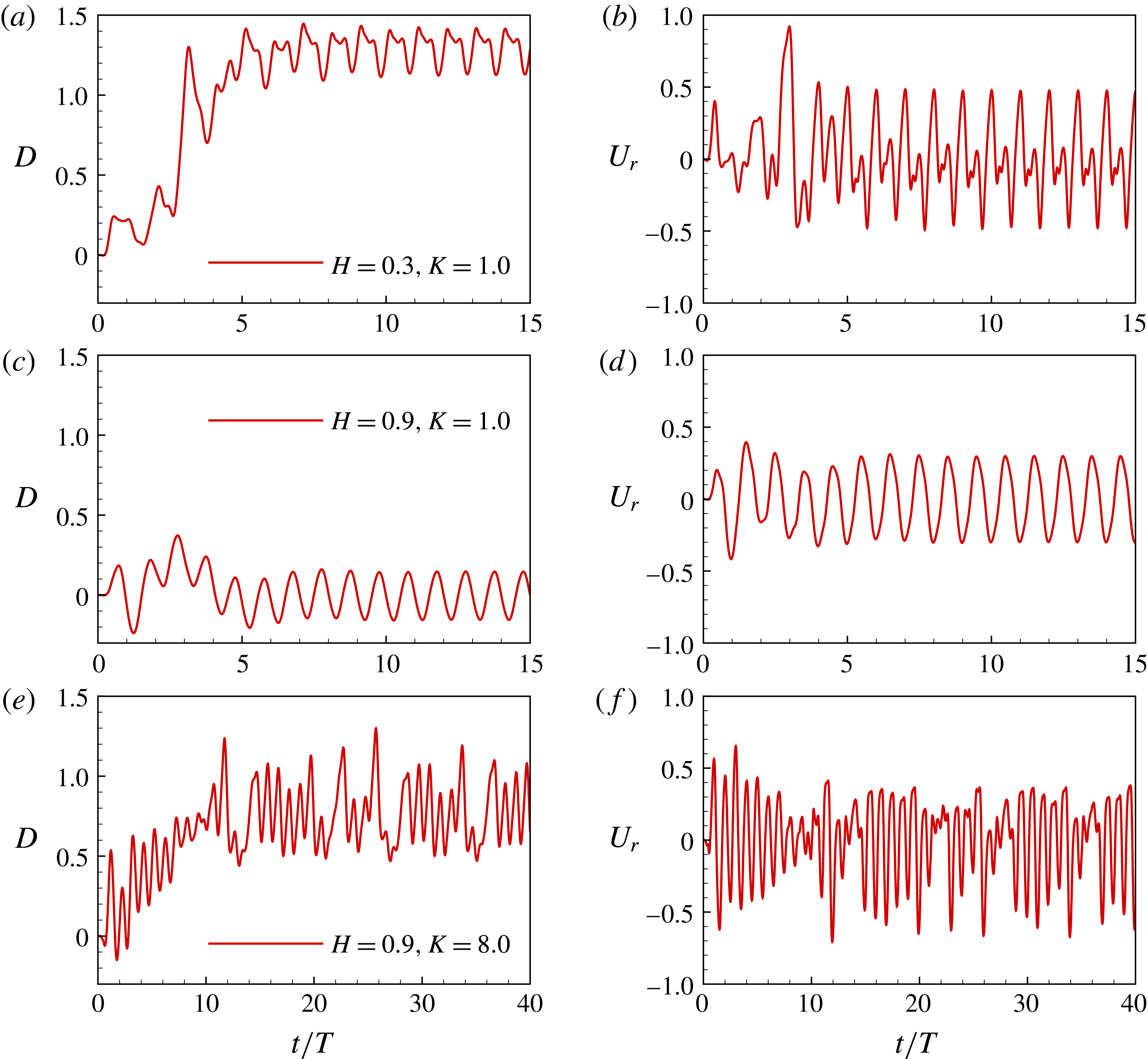
of the two plates (b,d,f) as a function of time. Panels (a,b), (c,d), and (e,f) correspond to the cases of the SF, AL and NP states, respectively. The key parameters
 $H$
and
 $K$
are labelled in (a,c,e).

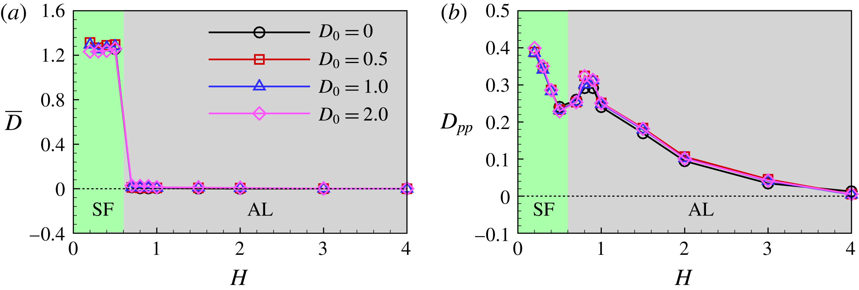
Time-averaged longitudinal spacing
 $\overline{D}$
(a) and the peak-to-peak value
 $D_{pp}$
(b) as functions of
 $H$
for the in-phase flapping. The effect of
 $D_{0}$
is also given.

Figure 4(a–d) shows the vorticity contours at four typical phases in one flapping cycle for the case with
 $H=0.3$
and
 $K=1$
, corresponding to the SF mode. In the SF state, the following plate moves forward following the leading plate with a staggered configuration. The two plates behave like one single and longer plate and the vortex street is behind the follower. The time histories of the longitudinal spacing
 $D(t)$
and relative propulsive speed
 $U_{r}(t)=u_{1}(t)-u_{2}(t)$
for the SF mode are shown in figure 5(a,b), where
 $u_{1}(t)$
and
 $u_{2}(t)$
are the instantaneous horizontal velocity of plate 1 and 2, respectively. It is seen that
 $D(t)$
and
 $U_{r}(t)$
evolve to periodic states with
 $\overline{D}\approx 1.3$
and
 $\overline{U}_{r}=0$
after a few flapping periods, where
 $\overline{D}$
and
 $\overline{U}_{r}$
are average values over one flapping period.
Figure 4(e,f,g,h) shows the vorticity contours in the AL mode. The reversed Kármán vortex street is clearly shown in the wake. The shedding vortex pattern is different from that in the SF mode. In the AL mode (
 $H=0.9$
),
 $D(t)$
changes periodically with
 $\overline{D}=0$
(see figure 5
c,d), indicating that during the propulsion, the two plates leapfrog or move forward in an alternate-leading way. When the plates become harder, the non-periodic (NP) mode appears. Figure 5(e,f) shows that in the NP mode,
 $D(t)$
and
 $U_{r}(t)$
vary non-periodically with time. It is noted that the lateral flow interactions between the two plates are negligible when the lateral distance is large enough, e.g.
 $H=4.0$
, which is referred to as the non-interfering state.
The time-averaged longitudinal spacing
 $\overline{D}$
and peak-to-peak value
 $D_{pp}$
as functions of
 $H$
for
 $K=1$
are shown in figure 6. It is seen that the collective pattern of the two-plate system switches from the SF mode to the AL mode as
 $H$
at
 $H_{c}\approx 0.6$
. It is worth noting that the peak-to-peak value of
 $D$
, i.e.
 $D_{pp}$
, is significant in the SF and AL modes, implying dynamic adjustment in the horizontal direction between individuals due to the flow-mediated interactions. Additionally,
 $D_{pp}$
tends to be zero due to the lateral interference vanishing as
 $H\geqslant 4$
.
To further examine whether the motion state can be maintained when the system is perturbed, the initial configurations are adjusted by varying the initial longitudinal spacing
 $D_{0}$
. Figure 6 also shows the results for
 $D_{0}=0.5$
, 1.0 and 2.0. It is seen that the ultimate stable configurations are mainly determined by
 $H$
but independent of
 $D_{0}$
when the horizontal disturbance is small (
 $D_{0}\leqslant 2.0$
). Hence, the formed configurations due to the fluid mediation are stable.
Passive flexibility of flapping plates, which is closely associated with their propulsive performance and wake properties (Hua et al.
Reference Hua, Zhu and Lu2013; Zhu et al.
Reference Zhu, He and Zhang2014b
), may play a key role in collective locomotion through the flow interactions between individuals. Thus, we further examine the effect of the flexibility on the two-plate system. In our numerical setting,
 $K$
ranges from
 $0.1$
(very flexible) to
 $10$
(very hard). In the simulations, the side-by-side initial configurations are adopted, i.e.
 $D_{0}=0$
and
 $H\in (0.2,6)$
.
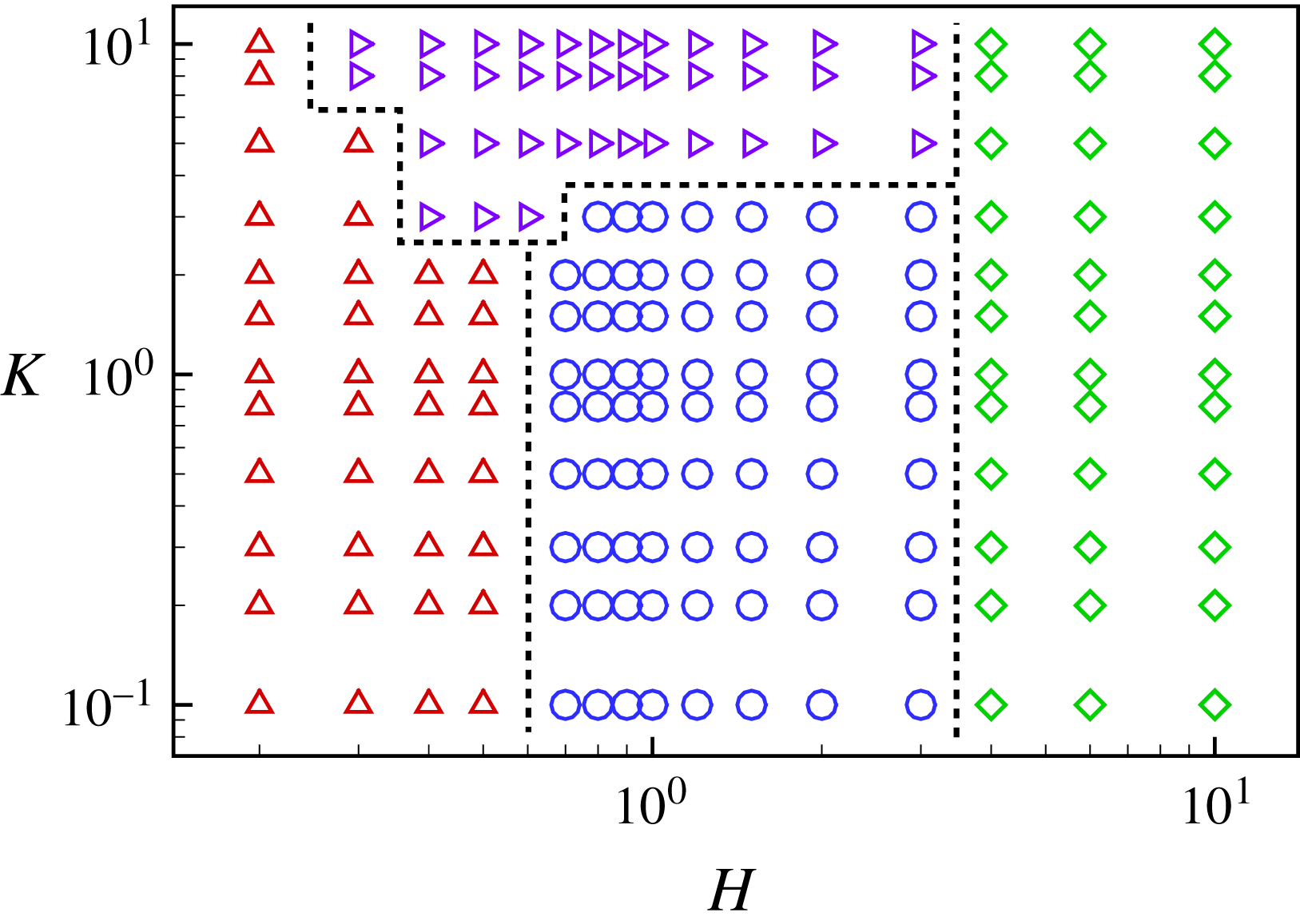
Phase diagram for the four motion states (
 $\unicode[STIX]{x1D719}=0$
). Symbols ▵, ○, ▹ and ♢ represent the SF, AL, NP and NI states, respectively.

Our results indicate that the occurrence of the locomotion states of the plates depends mainly on the bending stiffness
 $K$
and the lateral spacing
 $H$
. The phase diagram for the four modes in the
 $H$
–
 $K$
plane is shown in figure 7. Each point in the figure represents a case we simulated. We do not intend to provide accurate borders between the modes, therefore it is only a schematic diagram. It is seen that the SF state occurs mainly in the region with small
 $H$
. Both the AL and NP states mainly appear at moderate
 $H$
but the NP state covers the region with larger
 $K$
(say
 $K>2.0$
). When
 $H$
is large enough (say
 $H\geqslant 4.0$
), only the NI state occurs because the flow-mediated interactions between the two plates are negligible.
4.2 Plate performances in the SF state and the AL state
According to our simulations, stable configurations can be spontaneously formed. The propulsive properties of the plates in the SF and AL modes are further investigated. To quantify the propulsive performance of the plates, three important indicators, namely, the mean propulsive speed, input work and propulsive efficiency (Hua et al. Reference Hua, Zhu and Lu2013; Zhu et al. Reference Zhu, He and Zhang2014a ) are defined.
The mean propulsive speed
 $U$
is defined as the time-averaged forward speed at the equilibrium state, i.e.
 $$\begin{eqnarray}\displaystyle U=\frac{1}{T}\int _{t^{\prime }}^{t^{\prime }+T}u(t)\,\text{d}t=-\frac{1}{T}\int _{t^{\prime }}^{t^{\prime }+T}\left(\left.\frac{\unicode[STIX]{x2202}X}{\unicode[STIX]{x2202}t}\right|_{s=0}\right)\text{d}t, & & \displaystyle\end{eqnarray}$$
where
 $T$
is the flapping period. The input work
 $W$
is required to maintain the self-propulsion of the flapping plates. It is computed as a time integral of the power
 $P$
performed by the surface of the body on the surrounding fluid over one flapping period, i.e.
 $$\begin{eqnarray}\displaystyle W=\int _{t^{\prime }}^{t^{\prime }+T}P(t)\,\text{d}t=\int _{t^{\prime }}^{t^{\prime }+T}\left[\int _{0}^{1}\boldsymbol{F}_{r}(s,t)\boldsymbol{\cdot }\frac{\unicode[STIX]{x2202}\boldsymbol{X}(s,t)}{\unicode[STIX]{x2202}t}\,\text{d}s\right]\text{d}t, & & \displaystyle\end{eqnarray}$$
where
 $\boldsymbol{F}_{r}$
represents the force on the surrounding fluid by the plates. To quantify the propulsive efficiency of a self-propulsive body, the ratio of the kinetic energy of the body and the input work has been employed. Therefore the propulsive efficiency is
 $$\begin{eqnarray}\displaystyle \unicode[STIX]{x1D702}={\textstyle \frac{1}{2}}MU^{2}/W. & & \displaystyle\end{eqnarray}$$
The propulsive properties of the plates for the in-phase (
 $\unicode[STIX]{x1D719}=0$
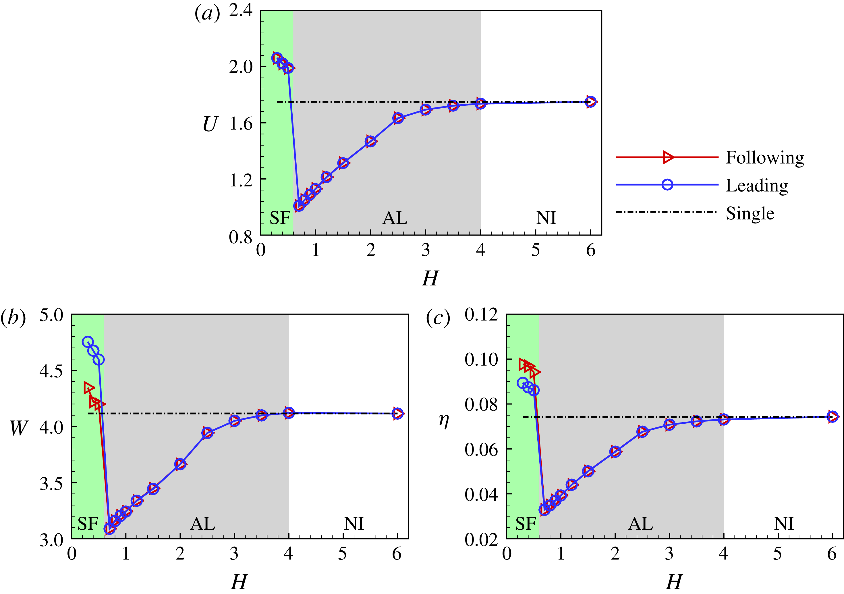
) scenario are presented in figure 8. It is seen that there are three propulsion modes (the NI, AL and SF states, respectively) as
 $H$
decreases from 6.0 to 0.2 for
 $K<2.0$
. Figure 8(a) shows the mean propulsive speed
 $U$
versus
 $H$
at the typical bending stiffness
 $K=1$
, which is an optimal
 $K$
for an isolated flapping plate. The mean propulsive speed of an isolated plate with
 $K=1$
is also shown by the dot-dashed line for comparison. When
 $H>4.0$
(the NI state), the mean propulsive speed
 $U$
is very close to that of the isolated plate. In the AL mode,
 $U$
decreases with
 $H$
monotonically and reaches the lowest point at
 $H\approx 0.6$
. As
 $H$
decreases further, the plates switch to the SF state, and
 $U$
becomes significantly larger than that of the isolated plate.
Propulsive speed
 $U$
(a), input work
 $W$
(b) and propulsive efficiency
 $\unicode[STIX]{x1D702}$
(c) as functions of
 $H$
for
 $K=1$
and
 $\unicode[STIX]{x1D719}=0$
. The green, grey and white regions represent the SF, AL and NI states, respectively.

Further, the input work and the propulsive efficiency as a function of
 $H$
are shown in figure 8(b,c). In the AL mode, the input work
 $W$
and propulsive efficiency
 $\unicode[STIX]{x1D702}$
of the plates are lower than those of the isolated one, while they jump to higher level in the region of the SF mode. It suggested that the flow-mediated interactions between the plates may be very different for the AL and SF states. Moreover, in the SF state, the plates have identical propulsive speed. Compared with the leading plate, the following one uses less input work (see figure 8
b) and therefore achieves higher propulsive efficiency (see figure 8
c). Hence, the SF configuration achieves better propulsive performance, and the follower can take advantage of the vortex shedding from the leading one in this compact configuration.
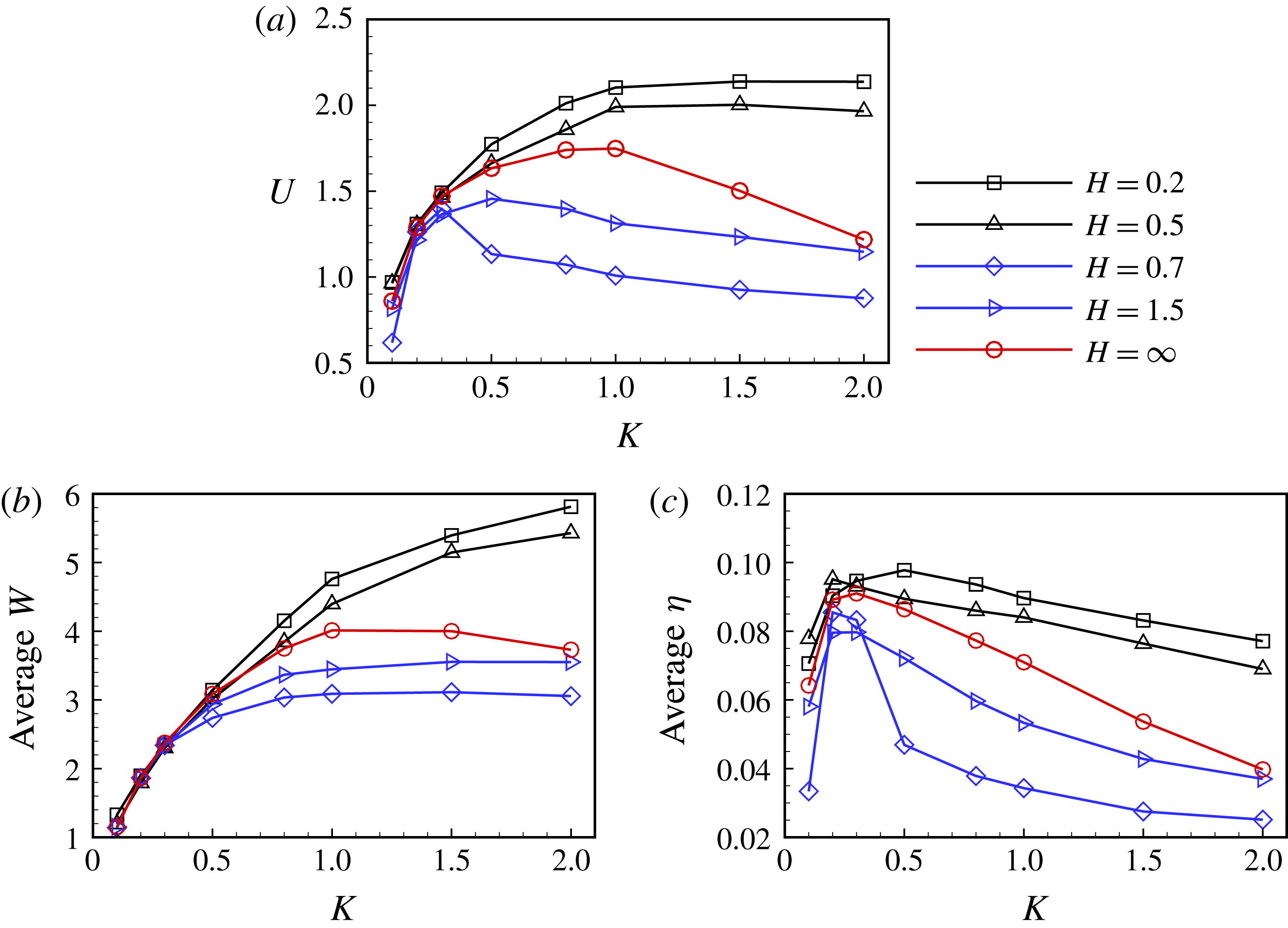
Propulsive speed
 $U$
(a), average input work
 $(W_{1}+W_{2})/2$
(b) and average propulsive efficiency
 $(1/2)M(U_{1}^{2}+U_{2}^{2})/(W_{1}+W_{2})$
(c) as functions of
 $K$
for different
 $H$
(
 $\unicode[STIX]{x1D719}=0$
).

The effect of
 $K$
on the performance is shown in figure 9. The average values of input work and propulsive efficiency of the two plates are calculated to evaluate the performance of the two-plate system, i.e.
 $(W_{1}+W_{2})/2$
and
 $(1/2)M(U_{1}^{2}+U_{2}^{2})/(W_{1}+W_{2})$
, respectively. It is seen that, compared to the isolated plate (
 $H=\infty$
), the propulsive performance of the plates is significantly improved as
 $K$
increases when
 $K>0.6$
for
 $H=0.2$
and 0.5. However, for
 $H=0.7$
and 1.5, the propulsive speed and efficiency of the plates decrease with
 $K$
when
 $K>0.3$
. It is also noted that when
 $K>2.0$
, the mode switches to the non-periodic mode and it is not possible to calculate the average values of
 $U$
,
 $W$
and
 $\unicode[STIX]{x1D702}$
according to their definitions. Hence, there are no data for
 $K>2.0$
.
4.3 Plate performance in the SF mode and the tandem case
For the two in-phase flappings, in this section we will discuss whether the performance in the staggered following is better than the simple tandem case (
 $H=0$
). In the simulations of the simple tandem case,
 $H=0$
is considered. For the staggered cases, five cases with
 $H=0.1{-}0.5$
are simulated. In the cases of
 $H=0$
, 0.1 and 0.2, the initial longitudinal spacing
 $D_{0}=1.1$
is adopted to avoid collisions. As mentioned above, in all of the simulations, the ultimate longitudinal spacing
 $D$
is independent of
 $D_{0}$
(see figure 6). For the five cases with
 $H\in [0.1,0.5]$
, the plates adopt the staggered-following mode with the specified lateral distance
 $H$
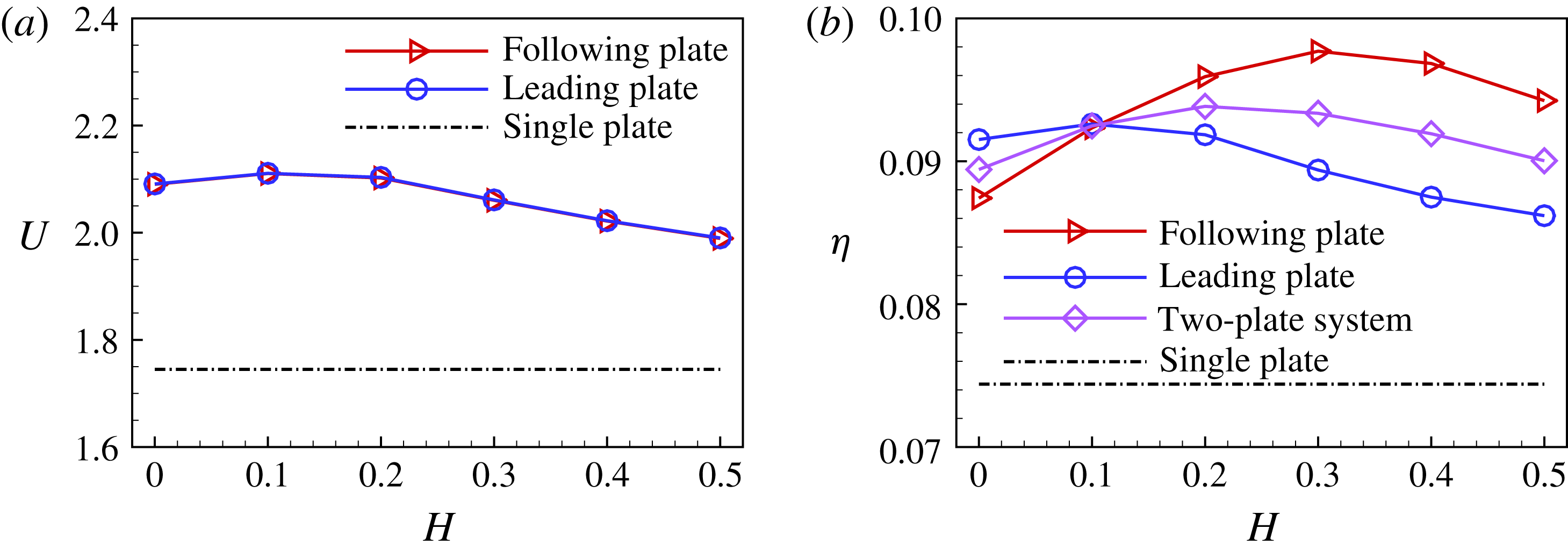
. Figure 10(a,b) shows the propulsive speed
 $U$
and efficiency of the plate
 $\unicode[STIX]{x1D702}$
for the tandem case
 $(H=0)$
and staggered cases
 $(H\in [0.1,0.5])$
. It is seen from figure 10(a) that the propulsive speed in the case of
 $H=0.1$
, as well as that in the case of
 $H=0.2$
, is somewhat higher than that of the simple tandem case.
Propulsive speed (a) and efficiency (b) of the plates for the simple tandem configuration
 $(H=0)$
and staggered configurations
 $(H=0.1{-}0.5)$
.

Figure 10(b) shows that at
 $H\approx 0.2$
the two plates achieve the optimal overall efficiency, which is better than that of the tandem case. It is also seen that in the tandem case (
 $H=0$
), the efficiency of the leading plate is higher than that of the following one. In this situation it seems that the leading plate can take advantage of the front–rear flow-mediated interaction. However, for the staggered cases with
 $H=0.2,0.3,0.4,0.5$
, the following plate can take more advantage than the leading one from the flow-mediated interaction. It is noted that there is an intermediate situation, i.e. at
 $H=0.1$
, the efficiencies of the two plates are almost identical.
For cases with multiple swimmers, e.g. four fish in Ashraf et al. (Reference Ashraf, Bradshaw, Ha, Halloy, Godoy-Diana and Thiria2017), it seems that the swimmers adopt the SF mode rather than the tandem configuration. The possible reason is that in view of hydrodynamics, the overall efficiency is optimized at the compact staggered configuration, e.g. the case of
 $H=0.2$
. The follower energy saving due to the flow-mediated interaction in the SF mode also matches well with the actual observation about follower’s egoism (Landa Reference Landa1998). In summary, for the in-phase flapping, the compact staggered configuration with a small lateral spacing is preferred for the propulsive performance in comparison with the tandem case.
4.4 Forces and powers
In the following, the forces experienced by the plates and the produced power are analysed to reveal the propulsion mechanism. It is noticed that, although the plates experience the net drag or thrust in the
 $x$
-direction due to the fluid–structure interactions at a specific time, the time-averaged force over the cycle is zero. Previous studies (Thiria & Godoy-Diana Reference Thiria and Godoy-Diana2010; Ramananarivo, Godoy-Diana & Thiria Reference Ramananarivo, Godoy-Diana and Thiria2011) on the flapping flexible wing and plate have indicated that the flexible deformation plays an important role in the thrust and drag as a ‘shape factor’ that redistributes the contribution of the aero- or hydrodynamic forces in the direction of forward motion. Here we will explore quantitatively the flexible deformation influence on the distribution of thrust and drag and the role of the flow-mediated interactions in the collective motions.
The jump in the fluid force across the plate at a certain Lagrangian point, i.e.
 $\boldsymbol{F}_{s}$
can be decomposed into two parts: one is the normal force
 $\boldsymbol{F}^{n}$
in which the pressure component dominates, the other is the tangential force
 $\boldsymbol{F}^{\unicode[STIX]{x1D70F}}$
which comes from the viscous effects. These forces are defined as
 $$\begin{eqnarray}\displaystyle & \displaystyle \boldsymbol{F}_{s}=[-p\unicode[STIX]{x1D644}+\unicode[STIX]{x1D64F}]\boldsymbol{\cdot }\boldsymbol{n}=\boldsymbol{F}^{n}+\boldsymbol{F}^{\unicode[STIX]{x1D70F}}, & \displaystyle\end{eqnarray}$$
 $$\begin{eqnarray}\displaystyle & \displaystyle \boldsymbol{F}^{n}=(\boldsymbol{F}_{s}\boldsymbol{\cdot }\boldsymbol{n})\boldsymbol{n}=(F_{x}^{n},F_{y}^{n}), & \displaystyle\end{eqnarray}$$
 $$\begin{eqnarray}\displaystyle & \displaystyle \boldsymbol{F}^{\unicode[STIX]{x1D70F}}=(\boldsymbol{F}_{s}\boldsymbol{\cdot }\unicode[STIX]{x1D749})\unicode[STIX]{x1D749}=(F_{x}^{\unicode[STIX]{x1D70F}},F_{y}^{\unicode[STIX]{x1D70F}}), & \displaystyle\end{eqnarray}$$
where
 $\unicode[STIX]{x1D644}$
is the unit tensor,
 $\unicode[STIX]{x1D64F}$
the viscous stress tensor,
 $\unicode[STIX]{x1D749}$
the unit tangential vector toward the trailing edge,
 $\boldsymbol{n}$
the unit normal vector as shown in figure 11(a) in the schematic and
 $[~]$
denotes the jump in a quantity across the immersed boundary. The power
 $P$
can also be decomposed into the two parts:
 $P^{n}$
and
 $P^{\unicode[STIX]{x1D70F}}$
, which are contributed by
 $\boldsymbol{F}^{n}$
and
 $\boldsymbol{F}^{\unicode[STIX]{x1D70F}}$
, respectively, i.e.
 $$\begin{eqnarray}\displaystyle & \displaystyle P=\boldsymbol{F}_{s}\boldsymbol{\cdot }\boldsymbol{u}=P^{n}+P^{\unicode[STIX]{x1D70F}}, & \displaystyle\end{eqnarray}$$
 $$\begin{eqnarray}\displaystyle & \displaystyle P^{n}=\boldsymbol{F}^{n}\boldsymbol{\cdot }\boldsymbol{u}=P_{x}^{n}+P_{y}^{n}, & \displaystyle\end{eqnarray}$$
 $$\begin{eqnarray}\displaystyle & \displaystyle P^{\unicode[STIX]{x1D70F}}=\boldsymbol{F}^{\unicode[STIX]{x1D70F}}\boldsymbol{\cdot }\boldsymbol{u}=P_{x}^{\unicode[STIX]{x1D70F}}+P_{y}^{\unicode[STIX]{x1D70F}}, & \displaystyle\end{eqnarray}$$
where
 $P_{x}^{n}=F_{x}^{n}\cdot u$
,
 $P_{y}^{n}=F_{y}^{n}\cdot v$
,
 $P_{x}^{\unicode[STIX]{x1D70F}}=F_{x}^{\unicode[STIX]{x1D70F}}\cdot u$
and
 $P_{y}^{\unicode[STIX]{x1D70F}}=F_{y}^{\unicode[STIX]{x1D70F}}\cdot v$
. It is noted that to maintain the heaving motion at the leading edge of the plate, input power done by an external force is required to sustain the propulsion system. Suppose the input power is
 $P_{in}$
, we have
 $P_{in}+P_{x}^{n}+P_{y}^{n}+P_{x}^{\unicode[STIX]{x1D70F}}+P_{y}^{\unicode[STIX]{x1D70F}}=0$
.
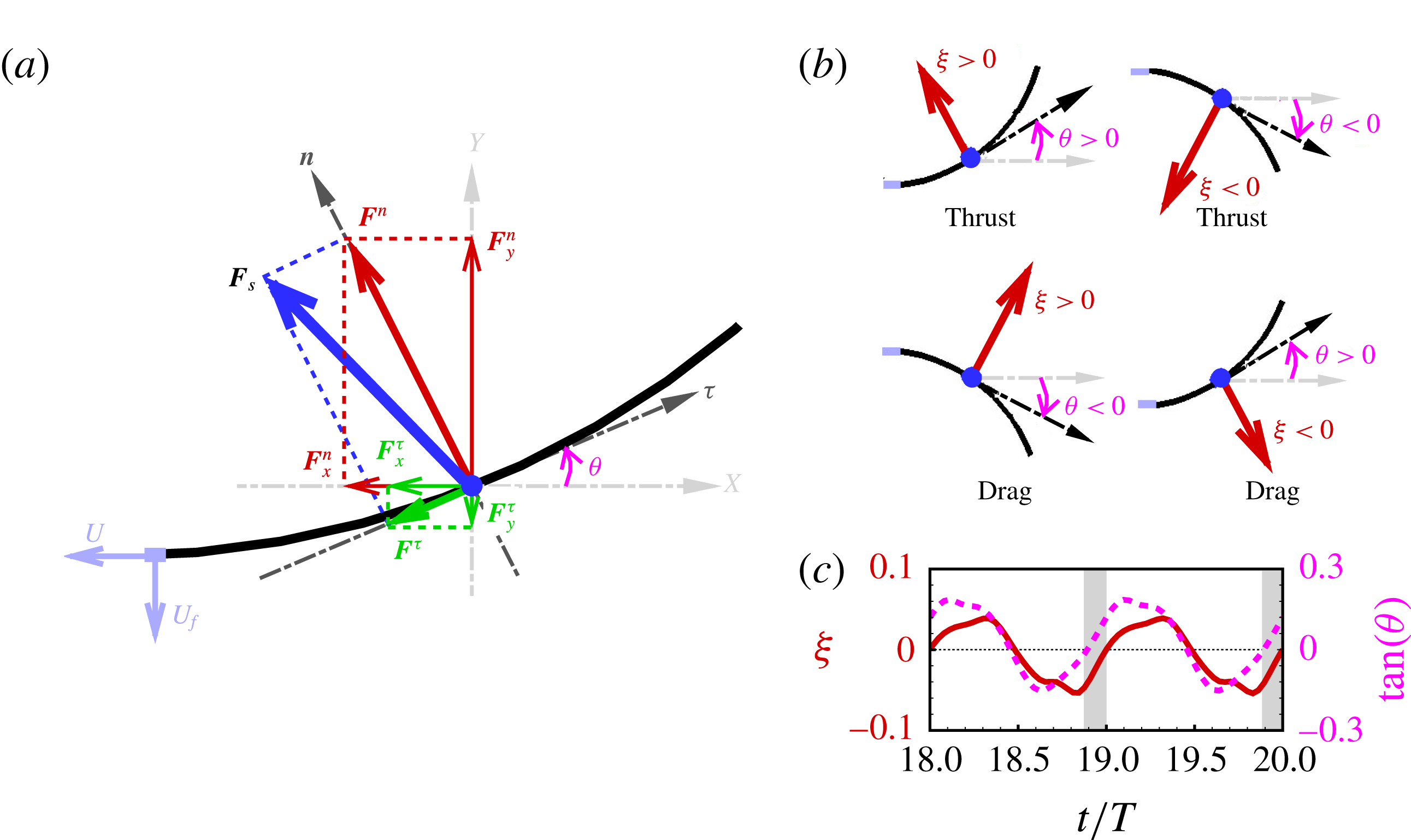
Schematic diagram for (a) force decomposition, (b) thrust generation, (c) phase difference between
 $\unicode[STIX]{x1D709}=\boldsymbol{F}_{s}\boldsymbol{\cdot }\boldsymbol{n}$
and
 $\tan \unicode[STIX]{x1D703}$
. Black curved lines represent the plate.
 $\unicode[STIX]{x1D749}$
and
 $\boldsymbol{n}$
denote the local tangential and normal vectors, respectively.

Figure 11(a) shows a schematic diagram of the force decomposition as mentioned above (see (4.4)–(4.6)). It is shown that the bending deformation of the flexible plate greatly influences the generation and distribution of
 $F_{x}^{n}$
due to different local geometry along the plate (Thiria & Godoy-Diana Reference Thiria and Godoy-Diana2010; Ramananarivo et al.
Reference Ramananarivo, Godoy-Diana and Thiria2011). Actually, the normal force contribution to the thrust or drag depends on the phase relation between the normal force and the local slope of the flexible plate (Mysa & Venkatraman Reference Mysa and Venkatraman2016). A schematic diagram to illustrate this point is shown in figure 11(b,c). In figure 11(b), it is seen that when the normal force and local slope at a certain point of the plate are simultaneously positive (
 $\unicode[STIX]{x1D709}=\boldsymbol{F}_{s}\boldsymbol{\cdot }\boldsymbol{n}>0$
and
 $\unicode[STIX]{x1D703}>0$
) or negative (
 $\unicode[STIX]{x1D709}<0$
and
 $\unicode[STIX]{x1D703}<0$
), the normal force contributes to a thrust; otherwise, the normal force contributes to a drag. Moreover, figure 11(c) shows the curves of
 $\unicode[STIX]{x1D709}$
and
 $\tan (\unicode[STIX]{x1D703})$
for a segment on the plate in two periods. From the periodic curves, the phase difference between them (
 $\unicode[STIX]{x1D6F9}$
) can be estimated to characterize the phase relation between the normal force and the local slope. When
 $\unicode[STIX]{x1D6F9}=0$
, they vary synchronously and the normal force contributes to a thrust force throughout the cycle. When
 $\unicode[STIX]{x1D6F9}=\unicode[STIX]{x03C0}$
, the normal force contributes to a drag instead of the thrust throughout the cycle. When
 $\unicode[STIX]{x1D6F9}\in (0,\unicode[STIX]{x03C0})$
, as shown in figure 11(c), the normal force contributes to a drag in the grey region and a thrust in the white region throughout the cycle.
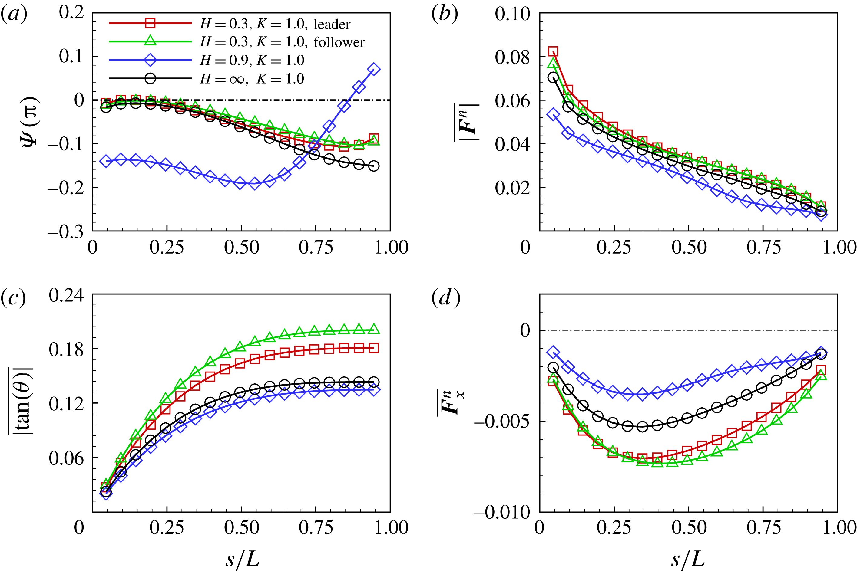
Phase difference, normal force and local slope along the flexible plates for the in-phase
 $(\unicode[STIX]{x1D719}=0)$
scenario. (a) Phase difference between normal force and slope, (b) time-averaged absolute normal force, (c) time-averaged absolute slope and (d) time-averaged
 $F_{x}^{n}$
. The forces are normalized by
 $F_{ref}=(1/2)\unicode[STIX]{x1D70C}U_{ref}^{2}L$
.

For the in-phase
 $(\unicode[STIX]{x1D719}=0)$
scenario, the deformation and thrust in the isolated case, the SF mode and the AL mode are compared in the follows. The phase difference, normal force and local slope along the flexible plates are presented in figure 12(a–c), respectively. Similar to the situation in the isolated case,
 $F_{x}^{n}$
contributes to the thrust for the SF and AL states in figure 12(d).
For the SF mode, figure 12(a) shows that the phase difference is closer to zero than that of the isolated case. Compared to the isolated case, it is seen that
 $\overline{|\boldsymbol{F}^{n}|}$
along the plate is slightly enhanced (see figure 12
b) and the local bending deformation increases significantly (see figure 12
c). All these features result in a larger thrust contributed by the normal force in the SF state. Compared to the leading plate, although the following plate experiences smaller
 $\overline{|\boldsymbol{F}^{n}|}$
in the anterior part, a larger bending deformation in the posterior part leads to a larger
 $\overline{F_{x}^{n}}$
in the posterior part. The overall
 $\overline{F_{x}^{n}}$
of the following plate is larger than that of the leading one.
For the AL state (
 $H=0.9,K=1.0$
), it is seen from figure 12 that, compared to the isolated case, the phase difference of the plate in the AL state (
 $\unicode[STIX]{x1D6F9}$
) is far from zero and the bending deformation (
 $\overline{|\text{tan}(\unicode[STIX]{x1D703})|}$
) as well as the normal force (
 $\overline{|\boldsymbol{F}^{n}|}$
) are slightly smaller. They all lead to a lower contribution of the normal force to the thrust in the AL state.
Integrating the total work along the whole plate, we obtain the total work of the following, leading and the isolated plates, which are 4.35, 4.75 and 4.12, respectively. While the work done by
 $F_{x}^{n}$
(the useful work) is approximately 1.80, 1.66, 1.01, respectively. It is seen that more useful work is achieved for each plate in the SF mode compared to the isolated case. Hence, the propulsive efficiency of the plates in the SF state is higher than that of the isolated plate in figure 8(c).
4.5 Flow structure and the unsteady dynamics
To better understand the mechanisms underlying the propulsive performance, the vortical structures around the plates and pressure distributions on the surfaces are investigated in the following.
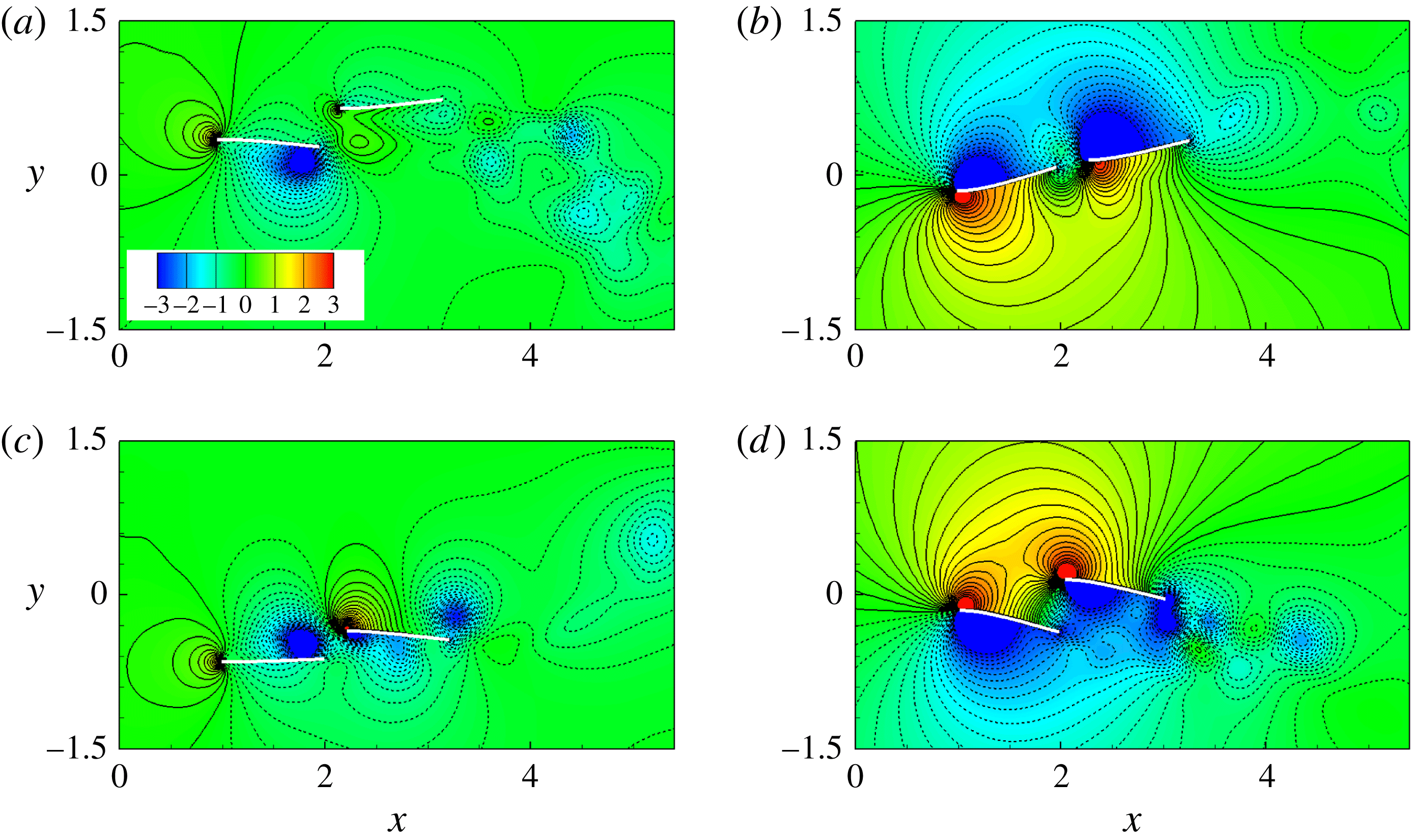
Instantaneous pressure contours at (a)
 $t=(0/4)T$
, (b)
 $T/4$
, (c)
 $(2/4)T$
and (d)
 $(3/4)T$
for the SF mode (
 $H=0.3$
,
 $K=1$
and
 $\unicode[STIX]{x1D719}=0$
). Solid and dashed lines denote the positive and negative normalized pressure contours, respectively.

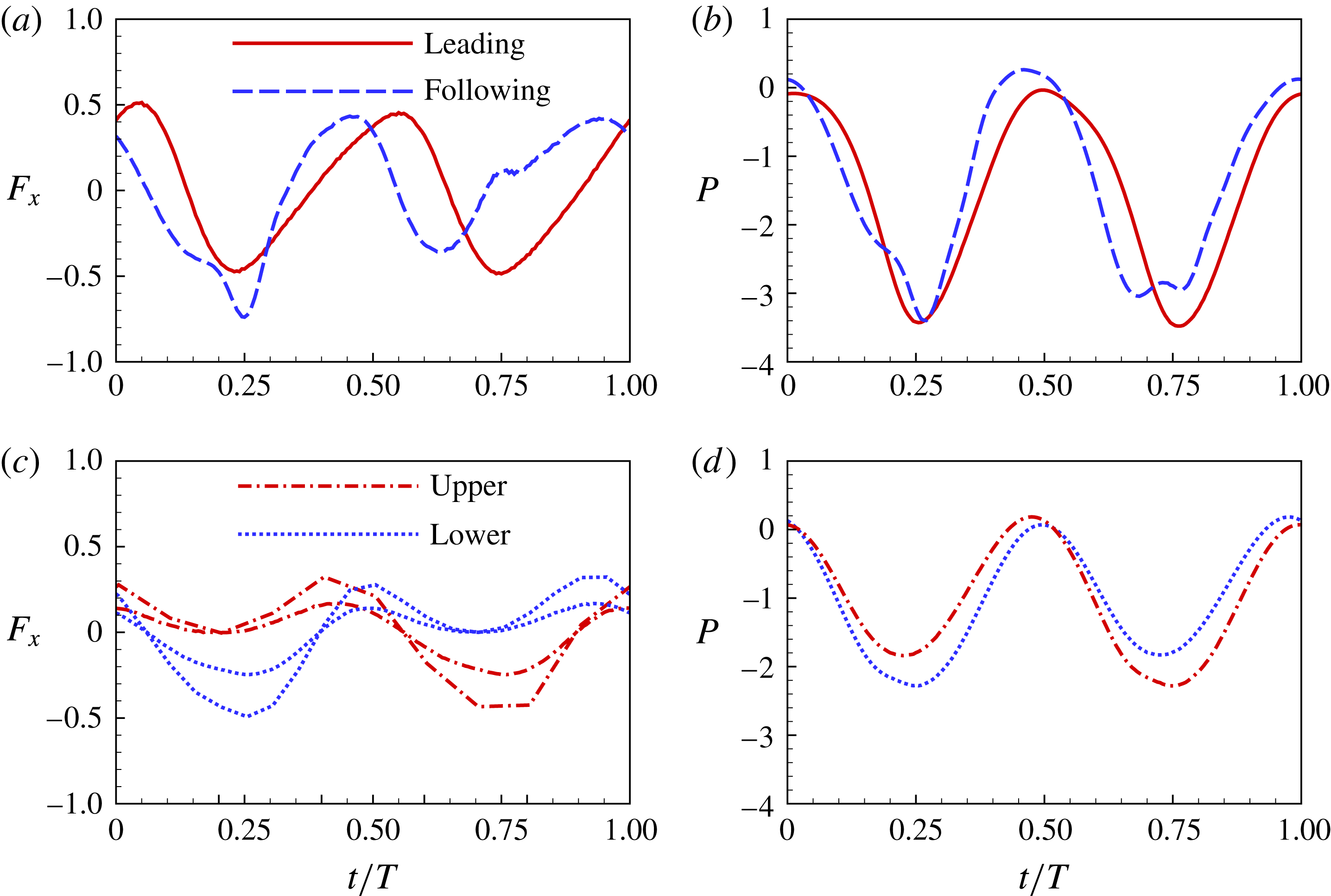
First, the instantaneous vorticity and pressure in the SF mode are analysed to understand how the flow-mediated interactions improve the propulsive performance. Figure 13 shows the pressure contours at typical instants of one flapping cycle. The two plates are propelled forward with a compact staggered configuration. From figure 13(a), it is seen that at the beginning of the down stroke, the thrust contributed by the normal force is negligible for the following plate because the pressure difference across the plate is small. The horizontal force in the SF mode is shown in figure 14. At
 $t=0$
, the forces
 $F_{x}$
of the two plates are almost identical.
Horizontal force experienced by the plates (a,c) and power of the plates (b,d) as functions of time in one period. Panels (a,b) and (c,d) represent the SF mode and the AL mode, respectively. The integration of the force in one period is zero. The forces and powers are normalized by
 $F_{ref}=(1/2)\unicode[STIX]{x1D70C}U_{ref}^{2}L$
and
 $P_{ref}=\unicode[STIX]{x1D70C}U_{ref}^{3}L$
, respectively.

At
 $t=T/4$
, figure 13(b) shows that the pressure difference across the following plate is approximately equal to that of the leading one. Therefore their thrusts contributed by the normal force are almost identical. On the other hand, the positive vortex shed from the leading plate extends to the lower surface of the following plate. Due to the vortex inducing effect, there are negative pressure contours ahead the following plate (Vandenberghe, Zhang & Childress Reference Vandenberghe, Zhang and Childress2004), which also contribute to a thrust (
 $F_{x}<0$
). Hence, the overall thrust of the following plate is larger than that of the leading plate (see figure 14
a).
Figure 13(c) shows that the pressure difference across each plate and the deformation of each plate are small at
 $t=T/2$
. The pressure difference between the head and tail of each plate induces the drag force. From figure 14(a), we can see that both plates experience drag forces (
 $F_{x}>0$
) at this moment. At
 $t=(3/4)T$
, it is seen from figure 13(d) that there are more positive pressure contours ahead of the following plate than that ahead of the leading plate, which result in a larger drag force. Although the pressure difference across each plate produces thrust, the overall horizontal force for the leading (following) plates is the thrust (drag) force, as shown in figure 14(a). The power of each plate is shown in figure 14(b). It is seen that the total work done by the leading plate is slightly larger than that of the following one during one period. On the other hand, the plates move with an identical mean propulsive velocity. Hence, the following flapping plate achieves better efficiency and takes advantage of the wake of the leading one.
The instantaneous vorticity and pressure in the AL mode are analysed here. From figure 4, it is seen that in the AL mode, the leading-edge vortex is generated and convected downstream along the plates per half-cycle, which is similar to that of an isolated swimming plate. At
 $t=(0/4)T$
, the leading edges of the plates reach their maximum vertical positions, the upper and lower surfaces of the plates induce positive and negative vorticity in figure 4(e), respectively. There is a low pressure area near the vortices region in figure 15(a). Meanwhile, the leading edges of the plates are subject to a considerable drag due to the presence of the local high pressure region ahead of the plates. At this moment, both plates experience a net drag (see figure 14
c). As the plates start to stroke down (
 $t=T/4$
), i.e. figure 15(b), because the normal force due to the pressure difference acting on the lower plate is larger, the thrust of the lower plate is larger than that of the upper plate (see figure 14
c). Due to the larger thrust, the laggard lower plate begins to chase the upper leading one.
Instantaneous pressure contours at (a)
 $t=(0/4)T$
, (b)
 $T/4$
, (c)
 $(2/4)T$
and (d)
 $(3/4)T$
for
 $H=0.9$
,
 $K=1$
and
 $\unicode[STIX]{x1D719}=0$
(the AL state). Solid and dashed lines denote the positive and negative normalized pressure contours, respectively.

When the plates stroke up, they experience the reverse procedure of the down stroke. In this way, the two plates would chase each other and achieve identical mean propulsive speed and efficiency over one flapping cycle. In the AL mode, compared to the isolated case, the normal force acting on each plate, and therefore the thrust, are reduced. Hence, the propulsive performance of each plate is poorer than that of the isolated case. The power of each plate is shown in figure 14(d). It is seen that the overall power is significantly smaller than that in the SF mode. The above mechanism is also simplified in § 4.6.2.
4.6 Antiphase
 $(\unicode[STIX]{x1D719}=\unicode[STIX]{x03C0})$
scenario

The phase difference between the swimmers may play an important role in forming the stable flow-mediated configurations and achieving collective advantages. For example, Ashraf et al. (Reference Ashraf, Bradshaw, Ha, Halloy, Godoy-Diana and Thiria2017) studied experimentally synchronization of tail-beating kinematics between neighbouring individuals within a group and found that fish swimming together at their free-ranging speed shows no consistent phase relationship between neighbours, which is consistent with the natural observations (Partridge & Pitcher Reference Partridge and Pitcher1979). On the contrary, fish in schools sustaining high swimming gaits shows strong synchronized dynamics, characterized by in-phase and out-of-phase (OP, or antiphase) modes (Ashraf et al. Reference Ashraf, Bradshaw, Ha, Halloy, Godoy-Diana and Thiria2017) and the OP mode is favoured with respect to the in-phase state (Ashraf et al. Reference Ashraf, Godoy-Diana, Halloy, Collignon and Thiria2016). Moreover, the antiphase undulating motions are usually considered as one of the typical cases in schools and investigated in the literature (e.g. Dong & Lu Reference Dong and Lu2007; Boschitsch et al. Reference Boschitsch, Dewey and Smits2014; Dewey et al. Reference Dewey, Quinn, Boschitsch and Smits2014). In this section the effects of the phase difference on the emergent dynamics and configurations are investigated.
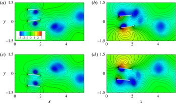
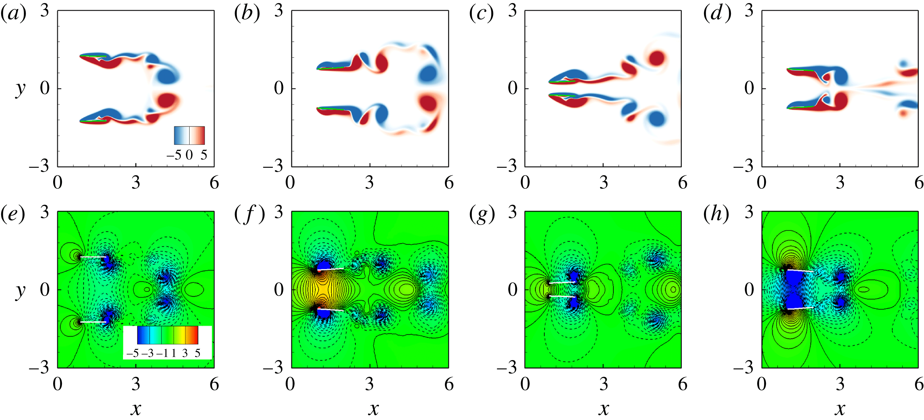
Instantaneous vorticity (a–d) and pressure (e–h) contours at (a,e)
 $t=(0/4)T$
, (b,f)
 $T/4$
, (c,g)
 $(2/4)T$
and (d,h)
 $(3/4)T$
from the left column to right for
 $H=1.5$
,
 $K=3.0$
in the antiphase scenario. Blue and red colours denote negative (clockwise) and positive (anticlockwise) vorticity, respectively. Solid and dashed lines for pressure contours denote the positive and negative normalized pressure contours.

In the current setting, the key parameters in our simulations are
 $\unicode[STIX]{x1D719}=\unicode[STIX]{x03C0},D_{0}=0,H=1.2{-}2$
and
 $K=1{-}10$
. In the antiphase scenario, the minimum value of
 $H$
is slightly larger than
 $2A$
to avoid collision of two plates. Two motion modes are identified based on our numerical results, i.e. the moving abreast (MA) mode and the AL mode. The instantaneous vorticity and pressure contours at
 $t=(0/4)T$
,
 $T/4$
,
 $(2/4)T$
and
 $(3/4)T$
are shown in figure 16. It is seen that in the MA mode,
 $D(t)=0$
and the propulsive velocities of the two plates are identical, i.e. the two plates move side-by-side with an identical speed. Besides, the instantaneous snapshots of the flow field and the geometries of the two plates at any time are symmetric about
 $y=0$
. For the AL motion state, the two plates move forward in an alternate-leading way.
4.6.1 Phase diagram and propulsive properties
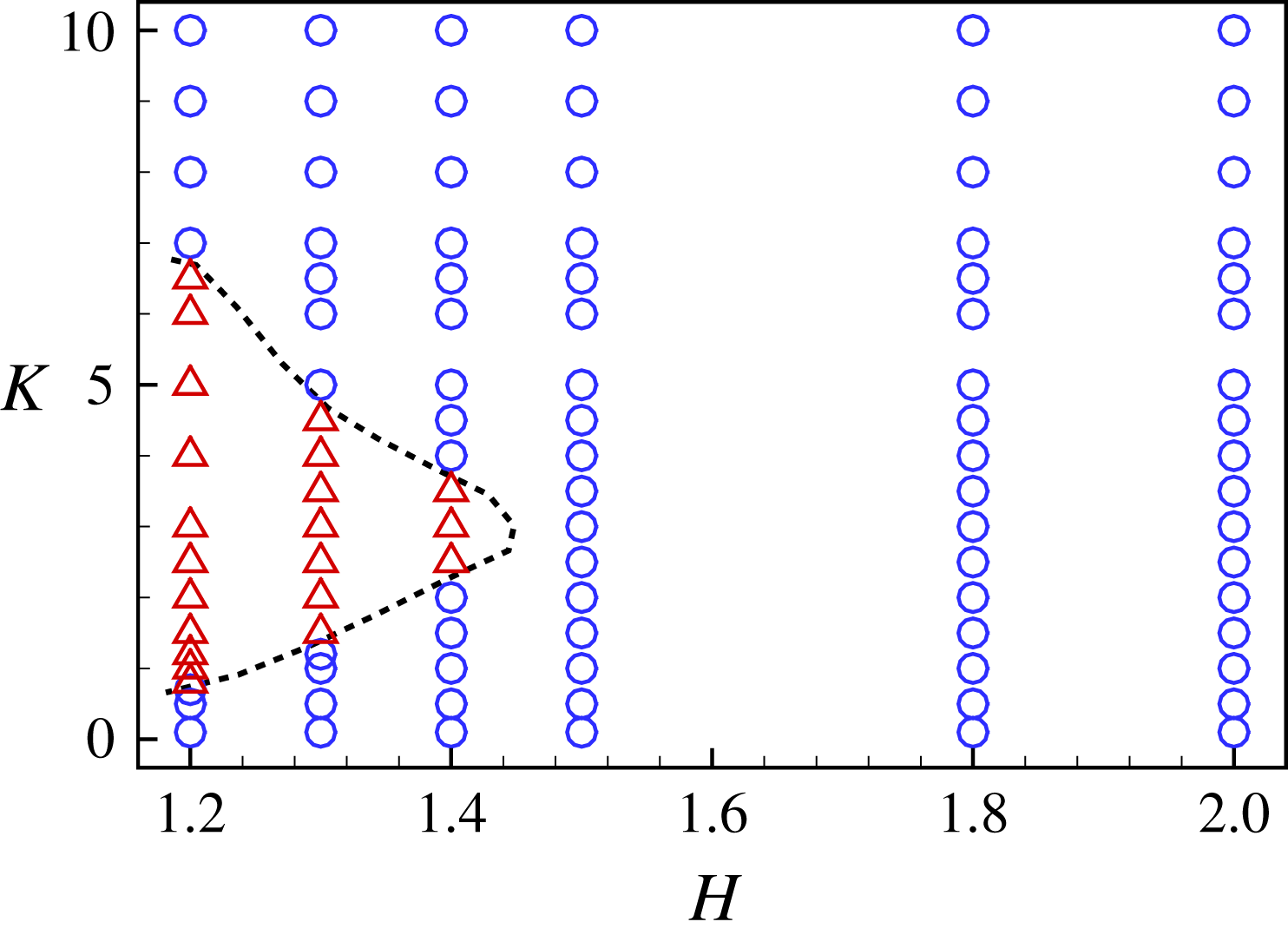
The phase diagram for the two motion modes are shown in figure 17. It is seen that in the
 $H$
–
 $K$
plane, the AL mode appears at the moderate bending stiffness
 $K$
with a small gap distance (
 $H<1.5$
). When the lateral distance
 $H$
is larger than 1.5, the AL mode disappears.
Phase diagram for the MA (○) and AL (▵) modes in the
 $H$
–
 $K$
plane for
 $\unicode[STIX]{x1D719}=\unicode[STIX]{x03C0}$
.

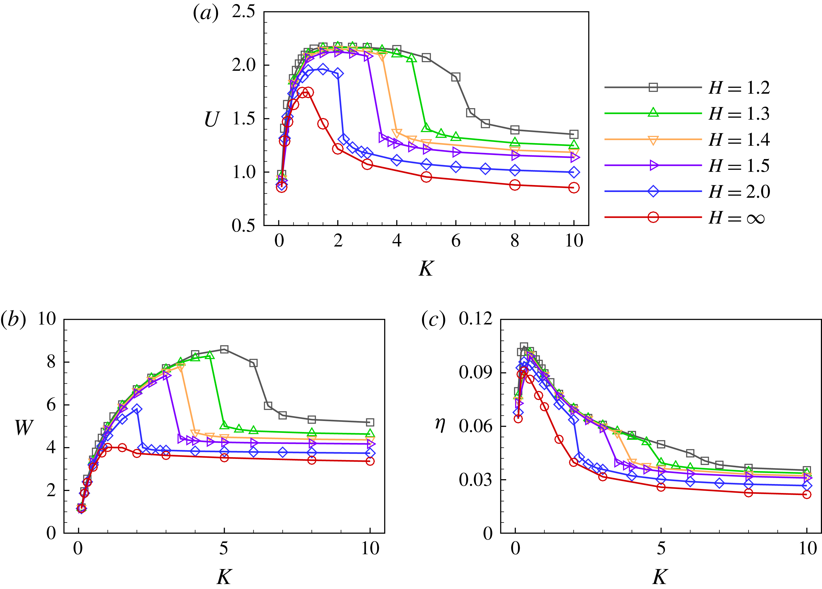
Mean propulsive speed
 $U$
(a), input work
 $W$
(b), propulsive efficiency
 $\unicode[STIX]{x1D702}$
(c) as functions of
 $K$
for varying
 $H$
(antiphase flappings).

In the antiphase (
 $\unicode[STIX]{x1D719}=\unicode[STIX]{x03C0}$
) scenario, the mean propulsive speed
 $U$
versus the bending stiffness
 $K$
for
 $H\in (1.2,2.0)$
is shown in figure 18(a). For each
 $H$
, the speed
 $U$
increases rapidly with
 $K$
first and reaches a plateau region with a maximum
 $U$
, then it decreases rapidly at a critical bending stiffness and finally approaches a constant. The plateau region for the maximum
 $U$
becomes narrower as
 $H$
increases from 1.2 to 2.0. Note that for
 $H=\infty$
, i.e. the isolated plate case, the plateau region narrows into a peak. Hence, short-range flow-mediated interactions (smaller
 $H$
) between the plates not only improve the propulsive speed, but also enlarge the range of optimal
 $K$
. Moreover, figure 18(b,c) shows the input work and the propulsive efficiency as functions of
 $K$
for
 $H\in (1.2,2.0)$
. The input work increases with
 $K$
first and decreases rapidly to a constant at a critical
 $K$
. For the propulsive efficiency, it increases to a peak at
 $K\approx 0.4$
and then decreases to a constant at the critical
 $K$
. The decreasing section can be understood in the following way. In the plateau region of propulsion speed
 $U$
(approximately
 $K\in (1,4)$
), the input work
 $W$
increases continuously to peak value. According to expression (4.3), it results in the decreasing propulsive efficiency. As a whole, figure 18 shows that the propulsive performance can be much improved when two closely spaced plates possess moderate flexibility.
4.6.2 Flow fields
Because the MA mode is able to achieve better propulsive performance, the vorticity and pressure contours of a typical MA case (
 $H=1.5$
and
 $K=3.0$
), that shown in figure 16, will be analysed first. In the following description, plate 1 (the upper plate) is taken as an example because the situation of plate 2 is symmetric to that of plate 1 about the line
 $y=0$
. From figure 16(a), it is seen that at the initial stage of down stroke of plate 1, the bending deformation increases to a maximum. The leading-edge positive vortex on the lower surface of plate 1 moves from the leading edge to the trailing edge, and interacts with the trailing-edge vortex. At
 $t=T/2$
in figure 16(b), all vortices are shed into the wake and the mutual induction among the vortices prevents them leaving vertically, which is helpful for the generation of thrust and improvement of propulsive efficiency (the detailed mechanism is shown in figure 19 and described in the next paragraph). Moreover, the high pressure region between the two plates grows when they stroke toward each other in figure 16(f), resulting in the enhancing normal force across the plates and the larger bending deformation. During the second half of the flapping cycle in figure 16(c,d,g,h), the vortices shed from the trailing edges move along the
 $x$
direction. The lower pressure region between two plates grows up gradually, which also enhances the normal force acting on the plate and the deformation of each plate, therefore the thrust increases. In the MA mode, the flow-mediated interactions contribute to a better propulsive performance as shown in figure 18.
Instantaneous vorticity contours for
 $K=3.0$
(a) and
 $K=3.5$
(b) in the antiphase scenario. The other parameters are
 $H=1.5$
and
 $\unicode[STIX]{x1D719}=\unicode[STIX]{x03C0}$
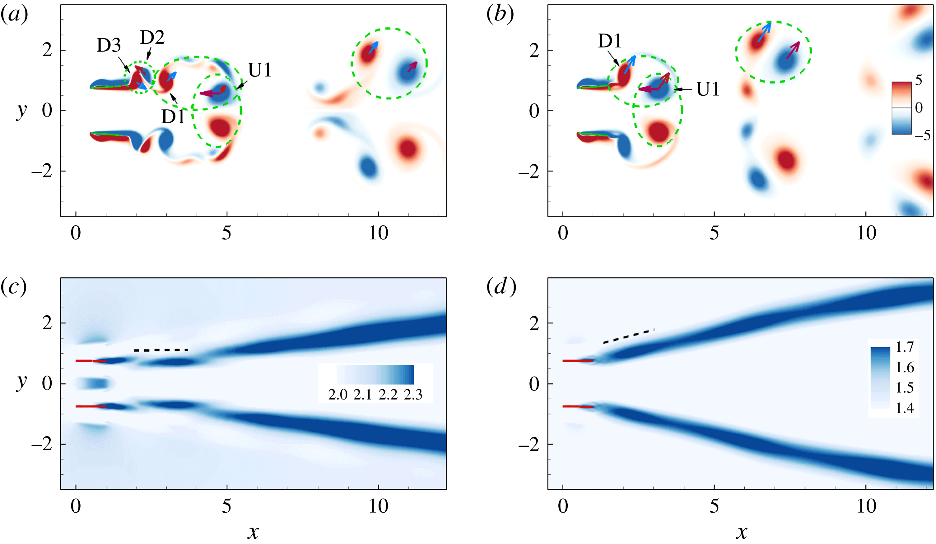
. Blue and red colours denote negative (clockwise) and positive (anticlockwise) vorticity, respectively. Red (blue) vectors represent the velocities induced by the neighbouring red (blue) vortices. Time-averaged jet in the wake for
 $K=3.0$
(c) and
 $K=3.5$
(d). The contours show the magnitude of adjusted horizontal velocity
 $\overline{u^{\prime }}=\overline{u}+U$
.

The vorticity contours at an instant for
 $K=3.0$
and
 $K=3.5$
are shown in figure 19. The induced velocity field around the vortices is also plotted in figure 19. It is seen that because the vortex ‘D1’ in figure 19(a) is weaker than that in figure 19(b) and the distance between vortices ‘U1’ and ‘D1’ in figure 19(a) is larger than that in figure 19(b), according to the Biot–Savart law, the induced lateral velocity acting on the ‘U1’ (the inclined vector) in the case of
 $K=3.0$
is smaller than that of ‘U1’ in the case of
 $K=3.5$
. Hence, the lateral movement of the vortices is slower in figure 19(a). In this way, it is seen clearly that the mutual induction among the vortices prevents them leaving vertically for the
 $K=3.0$
case. The comparison of the time-averaged jet in the wake for
 $K=3.0$
and
 $3.5$
is shown in figure 19(c,d). It is seen that the jet inclination angle for the
 $K=3.5$
case is approximately
 $15^{\circ }$
, which is larger than that in the
 $K=3.0$
case. This larger inclination angle is ‘a prognosticator of a further drop in thrust’ (Dong, Mittal & Najjar Reference Dong, Mittal and Najjar2006). Moreover, due to the small deformation of the plates in the case of
 $K=3.5$
, the thrust contributed by the normal force reduces significantly. Hence, the propulsive performance of
 $K=3.5$
becomes poorer.
Schematic diagrams for the pressure contours in (a) the MA (
 $\unicode[STIX]{x1D719}=\unicode[STIX]{x03C0}$
) and (b) AL (
 $\unicode[STIX]{x1D719}=0$
) modes, respectively. Solid and dashed contours denote the higher pressure region (HPR) and lower pressure region (LPR), respectively.

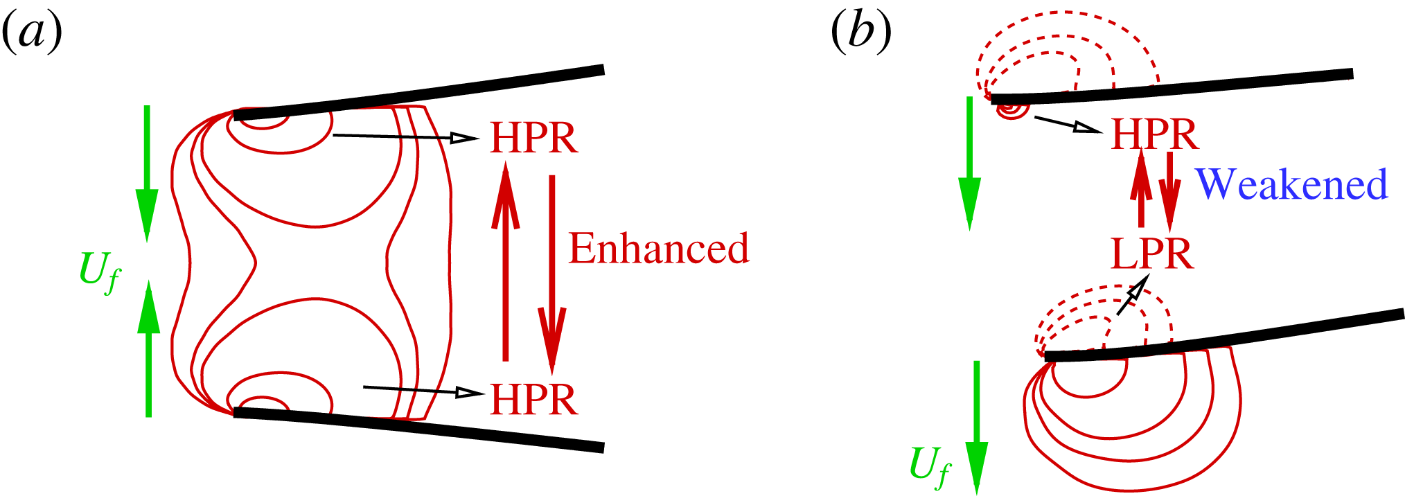
In summary, the propulsive performance of the side-by-side configuration due to the in-phase and antiphase flappings can be understood in the following way. Figure 20(a) shows that, as the plates flap in antiphase, when they are flapping close to each other, the pressure between them is enhanced significantly because the fluid between them is squeezed. Hence, the pressure difference between the upper and lower surfaces of each plate is larger than that in the isolated case. The larger pressure difference results in a larger deformation and normal force, and therefore a larger thrust. Similarly, when they are flapping apart from each other, the low pressure region between them also enhances the normal force acting on each plate. Hence the propulsive performance of each plate is enhanced compared to the isolated case. For the in-phase flapping (see figure 20 b), similar to the isolated plate, higher pressure or lower pressure is generated below or above each plate as it flaps downward. Hence, in the region between them, the higher pressure (HPR) generated by the flapping of plate 1 will interact with the lower pressure (LPR) generated by the flapping of plate 2. The HPR and LPR would weaken each other. Hence, the pressure difference between the upper and lower surfaces of each plate is not so large as that in the isolated case. The smaller pressure difference results in a smaller normal force, and therefore a smaller thrust. Then the propulsive performance is weakened.
4.6.3 Rescaling propulsive speed and efficiency
As discussed in the above, at moderate bending stiffness and small
 $H$
(e.g.
 $H=1.2$
), the thrust is mainly contributed by the normal force. Under this circumstance, the propulsive speed is enhanced and a better propulsive efficiency is achieved as shown in figure 18. It is also seen from figure 18(a,c) that for different
 $H$
, there exists a varying critical bending stiffness. When
 $K$
is beyond the critical value, the propulsive speed and efficiency of the plates decrease dramatically. For example, for
 $H=1.5$
the propulsive speed and efficiency decrease much as
 $K$
increases from 3.0 to 3.5. The possible reason is that the thrust contributed by the normal force is dominant in the case
 $H=1.5$
and
 $K=3.0$
. As
 $K$
increases to 3.5, the contribution of the normal force to the thrust reduces significantly due to the small deformation of the plates.
Rescaled propulsive speed (a) and efficiency (b) of the flapping plates as functions of rescaled bending stiffness for varying
 $H$
. Legend is identical to that in figure 18.

Generally speaking, the bending deformation of the flapping plate is dominated by the fluid dynamic pressure on the surface, inertial force of the plate and elastic restoring force due to the flexibility. Because the mass ratio
 $M$
is fixed at 0.2 in our simulation, the inertial force of the plate is very minor due to the small
 $M$
. Hence, the fluid force and the elastic restoring force should be estimated to determine the deformation.
To examine the relative importance of the two forces, the ratio of the elastic force to the fluid force is often used. Usually the ratio is quantified by the effective stiffness
 $K=EI/\unicode[STIX]{x1D70C}U_{ref}^{2}L^{3}$
. However, here the fluid dynamic pressure, i.e. the normal force, is more prominent. Hence, the normal force instead of
 $\unicode[STIX]{x1D70C}U_{ref}^{2}L$
is proposed to normalize the elastic force
 $EI/L^{2}$
directly, i.e.
 $K^{\ast }=EI/\overline{|\boldsymbol{F}^{n}|}L^{2}$
, which is referred to as an effective stiffness, where
 $\overline{|\boldsymbol{F}^{n}|}$
is the time-averaged absolute normal force of the plates over one flapping period. Moreover, the characteristic velocity is proposed to be
 $U_{ref}^{\ast }=(2\overline{|\boldsymbol{F}^{n}|}/\unicode[STIX]{x1D70C}L)^{1/2}$
, and thus the normalized propulsive speed is
 $U^{\ast }=U/U_{ref}^{\ast }$
.
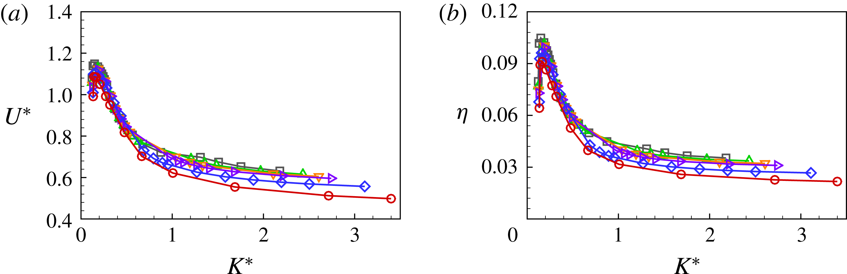
After the rescaling is performed, the propulsive speed
 $U^{\ast }$
and the efficiency
 $\unicode[STIX]{x1D702}$
of the antiphase flapping plates as functions of
 $K^{\ast }$
for different
 $H$
are shown in figure 21(a,b). From figure 21(a), it is seen that the plateaus with a maximum propulsive speed in figure 18(a) narrow into an identical peak at a critical value of
 $K^{\ast }\approx 0.25$
. Figure 21(b) shows that the curves of the propulsive efficiency also collapse together when
 $K^{\ast }$
is not too large. On the other hand, it is also noticed that the curves for different
 $H$
tend to deviate from each other slightly when
 $K^{\ast }$
is large. The possible reason is presented in the following. As discussed in the above, the thrust is primarily provided by the normal force for the plates with the moderate bending stiffness. While for the stiff plates, the thrust contributed by the normal force is not so significant due to the tiny deformation and the thrust is mainly induced by the leading-edge vortex. Therefore the scaling law based on
 $\overline{|\boldsymbol{F}^{n}|}$
is not so valid when
 $K^{\ast }$
is large. Hence, the rescaling works well only in the region of moderate
 $K^{\ast }$
.
4.7 Comparison with results in the literature
In the above, we concluded that under the circumstance of in-phase (IP) flapping, the SF mode is more efficient than the isolated case and the side-by-side case. However, for the antiphase (out-of-phase (OP)) flapping, the side-by-side is more efficient and there is no SF mode.
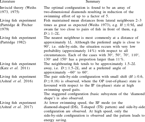
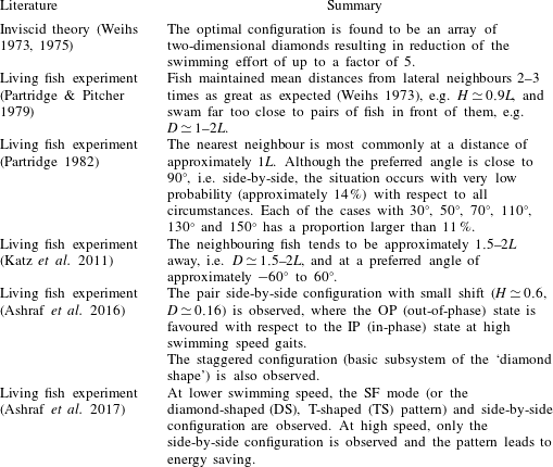
The optimal configurations for the two nearest neighbours in fish schooling are listed in table 2. It is seen that the SF mode in Katz et al. (Reference Katz, Tunstrøm, Ioannou, Huepe and Couzin2011) qualitatively agrees with our result about the SF mode. Besides, the SF cases have a very low distance
 $H<0.5$
(see figure 6) in terms of our simulation results. Movie S1 in Ashraf et al. (Reference Ashraf, Bradshaw, Ha, Halloy, Godoy-Diana and Thiria2017) also shows that the distance is
 $H\approx 0.35$
, which is consistent with our results for the SF mode. It is also seen that both side-by-side and staggered-following modes are found in Partridge (Reference Partridge1982) and when the side-by-side configuration appears, the OP (out-of-phase) state is favoured (Ashraf et al.
Reference Ashraf, Godoy-Diana, Halloy, Collignon and Thiria2016). Hence, some of our conclusions are basically consistent with the results in the literature.
Optimal configuration for two nearest neighbours. To quantify the orientation between a given fish and its nearest neighbour, the angle between the connected line of the two fish and the swimming direction is measured. Zero degrees is directly ahead of the fish;
 $180^{\circ }$
is directly behind.
It is also noticed that by using such a simple model it is impossible to fully reveal all hydrodynamic mechanisms of the fish schooling. There may exist some discrepancies between our results and those in the literature for the fish experiments. For example, the experimental study (Ashraf et al.
Reference Ashraf, Bradshaw, Ha, Halloy, Godoy-Diana and Thiria2017) showed that at the more energy-demanding, higher-velocity regimes, almost all schooling occurs in phalanx (side-by-side) formation. While in our simulations, not only the side-by-side formation but also the staggered formation (the SF mode) are found in the more energy-demanding, higher-velocity regimes. Another example is that Katz et al. (Reference Katz, Tunstrøm, Ioannou, Huepe and Couzin2011) and Ashraf et al. (Reference Ashraf, Bradshaw, Ha, Halloy, Godoy-Diana and Thiria2017) did not mention that the staggered arrangement leads to energy efficiency, while the SF mode in our study has higher efficiency. The inconsistency may be attributed to the limitation of our present model and the complexity of a natural fish school. As for the limitations of the present model, first our model consisting of two self-propulsion plates with simple actuation is a highly simplified model for a fish school. Second, it is only a two-dimensional study instead of three-dimensional. Third, the
 $Re$
is small with respect to the
 $Re$
regime of fish swimming.
It is worth mentioning that simulations/experiments from a limited number of bodies and at low
 $Re$
should be extended to a larger number and at high
 $Re$
with caution. In the present study, the wake interference of two self-propelled flapping plates at low
 $Re$
may not break the vortical structures into small structures and some coherent structures may still exist. At high
 $Re$
, although the wake of a single fish/object still shows coherent structures, wakes of many fish/object may become disorganized and the coherent structures may break down because of the interference of the wakes at high
 $Re$
(Daghooghi & Borazjani Reference Daghooghi and Borazjani2015).
5 Conclusions
The self-propulsion of two closely spaced flapping plates initially placed in a side-by-side configuration was investigated numerically. For the in-phase scenario, the four typical locomotion states of the plates have been identified according to their kinetic characteristics, i.e. the NI, AL, SF and NP states. The phase diagram for the states was presented. It is found that only in the SF state, the propulsive performance is enhanced compared to the case of isolated plate. The performance of the plates in the compact SF mode (small
 $H$
) is better than that in the tandem configuration (
 $H=0$
). Moreover, compared to the isolated case, both the plates in the SF mode swim much faster and have a higher efficiency although they consume more work
 $W$
. Furthermore, the following plate has a higher propulsive efficiency than the leading one, indicating that the following one takes advantage of the flow-mediated interaction. Force analysis shows that three factors are important to determine the thrust force, i.e. the normal force, the local slope of deformed plate and their phase difference. In the SF state, the flow-mediated interactions optimize the three factors and enhance the thrust and propulsive performance. In the AL mode, compared to the isolated case, the normal force acting on each plate is smaller than that of the isolated one. They lead to a poorer performance.
For the antiphase scenario, the MA and AL modes are observed. The MA mode is more common while the AL mode occurs only at moderate bending stiffness and small
 $H$
(
 $H<1.5$
). Investigations show that, provided
 $H$
is small, no matter in the AL or MA mode, the pressure difference across the plate and the bending deformation of each plate are enhanced, resulting in a larger thrust and improved propulsive performance at moderate stiffness. The normal force contributes much to the enhancement of performance. In summary, the higher efficiencies in the SF and MA modes relevant to the free swimming one is due to both the changes in kinematics and hydrodynamic interactions.
It is found there are plateau regions for the propulsive speed and the efficiency as functions of
 $K$
; when
 $K$
exceeds a critical value, the propulsive performance decreases dramatically. The propulsive speed and efficiency for antiphase flapping is rescaled using the time-averaged normal force as the characteristic parameter. The rescaling works well for the region with moderate bending stiffness, in which the normal force plays a critical role.
For two self-propelled plates, in view of hydrodynamics, to achieve higher performance the compact in-phase staggered-following mode and antiphase flappings in the side-by-side configuration are preferred. This study may shed some light on understanding coordinated collective behaviours in biological and natural systems.
Acknowledgements
This work was supported by the Natural Science Foundation of China (NSFC) grant nos 11372304 and 11621202. H.H. is supported by NSFC grant no. 11772326.