1. Introduction
The similarity hypotheses of Kolmogorov (Reference Kolmogorov1941a ,Reference Kolmogorov b , hereafter K41) constitute one of the few cornerstones in the subject of turbulence. Even so, Kolmogorov (Reference Kolmogorov1962, hereafter K62) himself had to refine his theory of ‘universal equilibrium’ (see also Obukhov Reference Obukhov1962) in order to account for departures from local isotropy due to the effects of spatial fluctuations of the energy dissipation rate. While these papers are admirably concise in themselves, it is hardly surprising that they continue to be the subject of much interest: excellent summaries with historical perspectives are provided by Kraichnan (Reference Kraichnan1974), Sreenivasan (Reference Sreenivasan1991), Sreenivasan & Antonia (Reference Sreenivasan and Antonia1997), Ishihara, Gotoh & Kaneda (Reference Ishihara, Gotoh and Kaneda2009) and Vassilicos (Reference Vassilicos2015).
The consensus view of local isotropy is that it relies on a wide separation of scales in order that the energy-containing scales do not influence the small-scale dissipating eddies, other than through the mean dissipation rate,
 ${\it\epsilon}$
. What exactly constitutes a ‘wide’ separation of scales has been the subject of much debate, and questions remain over the cause of high-wavenumber intermittency. A demonstration of a wide scale separation (but not necessarily of local isotropy) is the celebrated relationship attributed to Taylor (Reference Taylor1935),
 $$\begin{eqnarray}{\it\epsilon}=A_{1}\frac{u^{3}}{l},\end{eqnarray}$$
where
 $u$
and
 $l$
are, respectively, the velocity scale and length scale of the energy-containing turbulence and
 $A_{1}$
is a constant. It is widely acknowledged (but not universally accepted – see Davidson (Reference Davidson2004, p. 77)) that
 $A_{1}$
is a universal constant at asymptotically large Reynolds numbers. While the simulations of isotropic turbulence by Ishihara et al. (Reference Ishihara, Gotoh and Kaneda2009) show that
 $A_{1}$
asymptotes to a constant as the Taylor microscale Reynolds number
 $Re_{{\it\lambda}}\rightarrow 1200$
, they also show finite-Reynolds-number effects. The work of Vassilicos (Reference Vassilicos2015) and colleagues has considered the non-equilibrium effects of initial and large-scale conditions.
Equation (1.1) is an insufficient criterion for local isotropy because it is certainly the case that high-wavenumber intermittency increases with Reynolds number (or equivalently, with decreasing scale) as exemplified by the non-Gaussian behaviour of dissipation-related statistics (see Batchelor & Townsend Reference Batchelor and Townsend1949). Yet, little is known about the origins of intermittency and whether it might be attributable to the effects of Reynolds number, mean shear or solid boundaries, or whether it is intrinsic to the Navier–Stokes equations themselves (Kraichnan Reference Kraichnan1974). Ishihara et al. (Reference Ishihara, Gotoh and Kaneda2009) illustrate the importance of internal shear layers that lead to intermittency. Nor is it straightforward to separate out the effects of boundary conditions. Moreover, these hypotheses rely almost exclusively on experimental validation, which has always been limited by the relatively low Reynolds number available in most facilities. Sreenivasan & Antonia (Reference Sreenivasan and Antonia1997) emphasised the need for detailed measurements at high Reynolds numbers (
 $Re_{{\it\lambda}}>1000$
) of inertial range statistics in representative shear flows for which the large scales are well defined.
The spectral form of Kolmogorov (Reference Kolmogorov1941b
) – as postulated by Obukhov (Reference Obukhov1962) – has received support from many experiments both in the atmosphere and in the ocean (see e.g. Grant, Stewart & Moillet Reference Grant, Stewart and Moillet1962), both in the form of the inertial-subrange law as well as the collapse of spectra exhibiting universal equilibrium. Yet, questions remain and laboratory experiments in a single facility in which the boundary conditions are well controlled are few. Using an inertial-subrange scaling that enables use of a linear ordinate, Saddoughi & Veeravalli (Reference Saddoughi and Veeravalli1994) were able to show that the inertial subrange and local isotropy do not necessarily coincide – see also Mestayer (Reference Mestayer1982). Of the two decades exhibiting a
 $-5/3$
slope on log–log axes, only the higher one had a spectral shear correlation coefficient approaching zero. Durbin & Speziale (Reference Durbin and Speziale1991) show that an assumption of local isotropy is not justified even at high Reynolds numbers if the mean strain rate is not small, as suggested by Lumley (Reference Lumley1992). Bradshaw (Reference Bradshaw1967) identified a ‘first-order’ inertial subrange, for which a sufficient criterion is that energy sources or sinks are a small fraction of the spectral transfer. He identified
 $Re_{{\it\lambda}}>100$
to be a sufficient criterion for a wide range of flows, both with and without shear.
Both K41 and K62 theories are cast in the form of moments of velocity differences,
 $({\rm\Delta}u_{i})^{n}$
– since termed ‘structure functions’ by Monin & Yaglom (Reference Monin and Yaglom1975) – so that, in the direction
 $i$
,
 ${\rm\Delta}u_{i}=u_{i}(x_{i}+(r_{i}/2))-u_{i}(x_{i}-(r_{i}/2))$
for separation
 $r_{i}$
. Dual studies are limited, notable exceptions in shear flows being Saddoughi & Veeravalli (Reference Saddoughi and Veeravalli1994) and Mydlarski & Warhaft (Reference Mydlarski and Warhaft1996), among others. Many of the ambiguities associated with the definition of the
 $-5/3$
inertial-subrange law might be clarified by appeal to a unifying physical process.
Here, we explore the development of the inertial subrange in pipe flow by examination of the behaviour of moments of the longitudinal velocity structure function,
 $\langle ({\rm\Delta}u(r))^{n}\rangle$
, for Reynolds numbers (based on pipe diameter and bulk mean velocity,
 $\overline{U}$
) in the range
 $2.5\times 10^{5}<Re_{D}<6.0\times 10^{6}$
, that is, for
 $249\leqslant Re_{{\it\lambda}}\leqslant 986$
at the pipe centreline. For turbulent pipe flow, radius
 $R$
, the revisions in K62 may be expressed as:
 $$\begin{eqnarray}\frac{\langle ({\rm\Delta}u(r))^{n}\rangle }{{\it\upsilon}_{{\it\epsilon}}^{n}}=C_{n}\left(\frac{r}{{\it\eta}}\right)^{n/3}\left(\frac{r}{R}\right)^{-{\it\mu}_{n}},\end{eqnarray}$$
for
 ${\it\eta}\ll r\ll R$
, where
 ${\it\eta}=({\it\nu}^{3}/{\it\epsilon})^{1/4}$
is the Kolmogorov length scale,
 ${\it\upsilon}_{{\it\epsilon}}=({\it\nu}{\it\epsilon})^{1/4}$
is the Kolmogorov velocity scale and
 ${\it\nu}$
is the kinematic viscosity. The exponents
 ${\it\mu}_{n}$
and constants
 $C_{n}$
are undetermined and therefore require experimental estimation. They are presumed universal, although this is the source of some debate – see, for example, Sreenivasan (Reference Sreenivasan1995) and Sreenivasan & Antonia (Reference Sreenivasan and Antonia1997). Here,
 ${\it\mu}_{n}$
is a measure of the deviation of the exponent from the locally isotropic value,
 $n/3$
, and increases with
 $n$
. As might be expected, behaviour of the lower moments provides no information concerning the behaviour of the higher ones. Assuming a log-normal distribution for the dissipation averaged over a volume of linear dimension
 $r$
,
 ${\it\epsilon}_{r}$
, K62 gives
 $$\begin{eqnarray}{\it\mu}_{n}={\textstyle \frac{1}{18}}{\it\mu}n(n-3),\end{eqnarray}$$
where
 ${\it\mu}$
is supposedly universal. Its physical significance is illustrated by the sixth-order moment, where the dissipation rate correlated over
 $r$
is proportional to
 $$\begin{eqnarray}\langle ({\rm\Delta}u(r))^{6}\rangle \sim \left(\frac{R}{r}\right)^{{\it\mu}}.\end{eqnarray}$$
As
 ${\it\mu}>0$
always, (1.4) expresses the increase in the spatial intermittency with Reynolds number or, equivalently, a reduction in scale. Monin & Yaglom (Reference Monin and Yaglom1975) suggest
 ${\it\mu}\approx 0.4{-}0.5$
. They also provide the Fourier space equivalent to (1.2) as
 $$\begin{eqnarray}{\it\phi}_{11}(k_{1})=C{\it\epsilon}_{r}^{2/3}k_{1}^{-5/3}(k_{1}R)^{-{\it\mu}/9}\!.\end{eqnarray}$$
At the centreline, the transport equation for the turbulence kinetic energy reduces to
 $$\begin{eqnarray}-\frac{1}{{\it\zeta}}\frac{\text{d}}{\text{d}{\it\zeta}}\left[{\it\zeta}\left(\frac{1}{2}\overline{q^{2}v}+\frac{\overline{p^{\prime }v}}{{\it\rho}}\right)\right]={\it\epsilon},\end{eqnarray}$$
where
 ${\it\zeta}=R-y$
and in which the pressure transport term is the much smaller one of the two. At the centreline of fully developed pipe flow (no streamwise gradients), axisymmetry forces to zero radial gradients of even-order products only.
Scale-by-scale energy transfer is described by the Kármán–Howarth–Monin equation (Monin & Yaglom Reference Monin and Yaglom1975; Frisch Reference Frisch1995) for the second-order structure function. Assuming stationary, homogeneous (but not isotropic) fully developed flow at the pipe centreline, it reduces to a balance between inertial energy transfer, viscous diffusion and dissipation (Marati, Casciola & Piva Reference Marati, Casciola and Piva2004). With the assumption of local isotropy, integration yields Kolmogorov’s equation:
 $$\begin{eqnarray}-\langle ({\rm\Delta}u)^{3}\rangle +6{\it\nu}\frac{\text{d}}{\text{d}r}\langle ({\rm\Delta}u)^{2}\rangle =\frac{4}{5}{\it\epsilon}r.\end{eqnarray}$$
In the inertial subrange, the viscous term may be assumed to be negligible (Saddoughi & Veeravalli Reference Saddoughi and Veeravalli1994; Antonia, Zhou & Romano Reference Antonia, Zhou and Romano1997; Antonia & Burattini Reference Antonia and Burattini2006) and Kolmogorov’s four-fifths law is obtained:
 $$\begin{eqnarray}\langle ({\rm\Delta}u)^{3}\rangle =-{\textstyle \frac{4}{5}}{\it\epsilon}r.\end{eqnarray}$$
Hence, in addition to the dissipation rate, an isotropic estimate of the enstrophy may be of interest.
Equation (1.6) also indicates that exact isotropy cannot be consistent with stationarity at any Reynolds number because the turbulent transport in (1.6) appears in the spectral budget as a source or a sink at each wavenumber. This makes the case for a close examination of the additional spectral transfer arising through scale inhomogeneity (Lumley Reference Lumley, Yaglom and Tatarski1967). Antonia et al. (Reference Antonia, Zhou and Romano1997) show that
 ${\it\epsilon}_{iso}/{\it\epsilon}\approx 0.95$
for simulated channel flow at low Reynolds number (
 $Re_{{\it\tau}}=395$
). Therefore, in the present measurements at much higher Reynolds numbers, we take the four-fifths law as a reasonably accurate estimate of centreline dissipation rate. Danaila et al. (Reference Danaila, Anselmat, Zhou and Antonia2001) have proposed a generalised form of Kolmogorov’s equation to account for the effects of large-scale transport in fully developed channel flow appearing through the left-hand side of (1.6). However, the additional term involves the longitudinal structure function for the wall-normal fluctuations.
2. Experimental techniques
Measurements were performed in the Princeton/ONR Superpipe using NSTAP probes of length
 $\ell =30~{\rm\mu}\text{m}$
or
 $60~{\rm\mu}\text{m}$
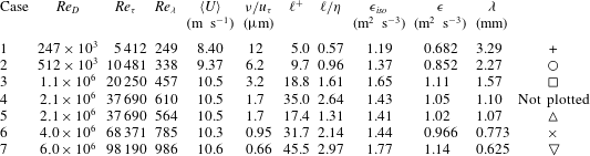
, with temporal resolution up to 300 kHz. The datasets from which the present results derive (
 $250\times 10^{3}\leqslant Re_{D}\leqslant 6.0\times 10^{6}$
) are those previously reported by Vallikivi et al. (Reference Vallikivi, Hultmark, Bailey and Smits2011), Hultmark et al. (Reference Hultmark, Vallikivi, Bailey and Smits2013), Rosenberg et al. (Reference Rosenberg, Hultmark, Vallikivi and Smits2013) and Vallikivi (Reference Vallikivi2014). Structure functions (up to third-order moments) and spectra are calculated using time series of either 60 s or 90 s duration: the latter have previously been presented by Rosenberg et al. (Reference Rosenberg, Hultmark, Vallikivi and Smits2013), and their scaling at lower wavenumbers examined by Vallikivi, Ganapathisubramani & Smits (Reference Vallikivi, Ganapathisubramani and Smits2015). Full details of the experiments appear in Vallikivi (Reference Vallikivi2014).


Dissipation spectra (see Rosenberg et al.
Reference Rosenberg, Hultmark, Vallikivi and Smits2013, figure 3) show two decades of inertial subrange. All data conform to the criterion for a ‘first-order’ subrange proposed by Bradshaw (Reference Bradshaw1967),
 $Re_{{\it\lambda}}>100$
. Note that all spectra extend beyond both the noise floor and the viscous cut-off. An isotropic estimate of
 ${\it\epsilon}$
is calculated by integration of the dissipation spectra,
 $$\begin{eqnarray}{\it\epsilon}_{iso}=15{\it\nu}\int _{0}^{\infty }k_{1}^{2}{\it\phi}(k_{1})\,\text{d}k_{1},\end{eqnarray}$$
up to the frequency at which the noise floor is determined and taken to be the minimum of the spectral estimate. At the highest Reynolds number
 $Re_{D}=6\times 10^{6}$
, the Kolmogorov length scale
 ${\it\eta}\approx 10~{\rm\mu}\text{m}$
, equivalent to
 $l=3{\it\eta}$
, or
 $k_{1}{\it\eta}|_{max}\approx 2$
: note that the dissipation spectrum peaks at
 $k_{1}{\it\eta}\approx 0.1$
; see table 1. Inspection of the spectra shows that, at
 $Re_{D}=6\times 10^{6}$
, the noise floor appears at
 $k_{1}{\it\eta}\approx 0.5$
; at
 $Re_{D}=4\times 10^{6}$
, it appears at
 $k_{1}{\it\eta}\approx 0.7$
. Therefore it is likely that the spectra at the two highest Reynolds numbers are slightly under-resolved, suggesting that the estimate of dissipation is likely to be low. Vallikivi (Reference Vallikivi2014) estimates the errors associated with the spectral estimates of the dissipation rate in the range of 2–16 % increasing with Reynolds number. It is probably for this reason that
 ${\it\epsilon}$
does not converge to the value of
 ${\it\epsilon}_{iso}$
as Reynolds number increases.
3. Results
Analysis comprises a first and second pass: the first provides estimates of the first three moments through time averaging of velocity differences. The third moment is then used to calculate estimates of the dissipation rate using (1.8). The second pass is used to calculate probability density functions for the velocity differences and their moments up to arbitrary order. In what follows, for consistency, scaling of spectra is performed using dissipation rate estimates using (2.1), while scaling of structure functions is performed using estimates of dissipation rate from (1.8).


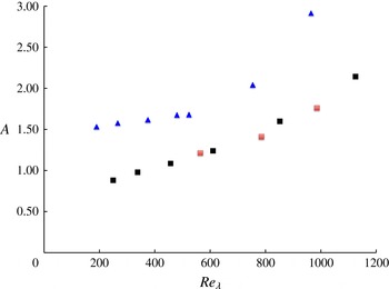
Figure 1 shows
 $A$
plotted as a function of
 $Re_{{\it\lambda}}$
, where
 ${\it\epsilon}=v_{{\it\epsilon}}^{3}/{\it\eta}=Au_{{\it\tau}}^{3}/R$
. Here,
 ${\it\epsilon}$
estimated using (1.8) is taken to be the maximum over a range of
 $r/{\it\eta}$
– this is made necessary by the nature of the third-order moments, which do not show a pronounced plateau, as shown below. It is noticeable that neither dissipation estimate provides values of
 $A$
that asymptote to a constant: rather
 $A$
increases almost linearly with
 $Re_{{\it\lambda}}$
. The ordinate is proportional to the estimate
 ${\it\epsilon}$
: therefore the increase in
 $A$
at higher Reynolds numbers cannot be attributed to poor spatial resolution. Furthermore, there is a remarkable consistency between estimates of
 $A$
using (1.8) obtained using the 30 and
 $60~{\rm\mu}\text{m}$
probes.
3.1. Kolmogorov (Reference Kolmogorov1941a ,Reference Kolmogorov b )
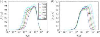
Figure 2 shows compensated inertial-subrange spectra where
 $k_{1}=2{\rm\pi}f/U$
is the streamwise wavenumber and
 $U$
is the local streamwise mean velocity. With inner, viscous scaling,
 $$\begin{eqnarray}f_{1}(k_{1}{\it\eta})={\it\epsilon}^{-2/3}k_{1}^{5/3}{\it\phi}_{11}(k_{1})=\frac{(k_{1}{\it\eta})^{5/3}}{v_{{\it\epsilon}}^{2}}{\it\phi}_{11}(k_{1}{\it\eta}),\end{eqnarray}$$
and with outer scaling,
 $$\begin{eqnarray}f_{2}(k_{1}R)={\it\epsilon}^{-2/3}k_{1}^{5/3}{\it\phi}_{11}(k_{1})=A^{-2/3}\frac{(k_{1}R)^{5/3}}{u_{{\it\tau}}^{2}}{\it\phi}_{11}(k_{1}R).\end{eqnarray}$$
At sufficiently large Reynolds number, classical subrange scaling gives
 $f_{1}(k_{1}{\it\eta})\rightarrow C$
and
 $f_{2}(k_{1}R)\rightarrow C$
where
 $C\approx 0.5$
(Monin & Yaglom Reference Monin and Yaglom1975). While
 $f_{1}$
collapses at high wavenumbers and
 $f_{2}$
collapses at low wavenumbers, there is no clear classical inertial-subrange scaling. Rather, both scalings suggest a more shallow slope than
 $-5/3$
: Vallikivi et al. (Reference Vallikivi, Ganapathisubramani and Smits2015) have previously reported that the inertial-subrange slope is closer to
 $-3/2$
than
 $-5/3$
. Interestingly, the simulations of isotropic turbulence by Ishihara et al. (Reference Ishihara, Gotoh and Kaneda2009) suggest a steeper spectral slope of
 $-5/3+{\it\mu}$
where
 ${\it\mu}\approx -0.1$
. Both sets of spectra in figure 2 show a ‘spectral bump’ at
 $k_{1}{\it\eta}\approx 0.05$
that could correspond to the ‘bottleneck phenomenon’ (Falkovich Reference Falkovich1994) – energy transfer arising from the viscous suppression of triadic interactions due to the rapid roll-off of the energy spectrum in the dissipation range. This phenomenon has also been shown by Saddoughi & Veeravalli (Reference Saddoughi and Veeravalli1994) and McKeon & Morrison (Reference McKeon and Morrison2007) at similar wavenumbers: however, it is difficult to discuss sensibly without first demonstrating a self-similar inertial subrange.


Structure functions, with
 ${\it\zeta}_{n}=n/3$
and
 ${\it\mu}_{n}=0$
: (a) second-order (
 $n=2$
) moments,
 $C_{2}$
; (b) third-order (
 $n=3$
) moments,
 $C_{3}$
.

Figure 3 shows second- and third-order structure functions: no smoothing over a range of values of
 $r$
is used. With increasing Reynolds number, both moments are characterised by a reduction in the ordinate value at small
 $r/{\it\eta}$
followed by increasing ordinate values at large
 $r/{\it\eta}$
. This gives the appearance of each plot line being rotated anticlockwise as the Reynolds number increases. For the second-order moment, K41 suggests that
 $C_{2}\approx 2.0$
in the inertial range (say,
 $30\lesssim r/{\it\eta}\lesssim 200$
): figure 3(a) indicates that the constant is Reynolds-number-dependent, even for
 $Re_{{\it\lambda}}>500$
. In figure 3(b), we expect a plateau in the inertial range, which in the limit of very large Reynolds number will asymptote to a constant of
 $4/5$
given by (1.8). However, no clear plateau is evident; instead a peak appears around
 $r/{\it\eta}\approx 60$
. Using a correction for finite Reynolds number (
 $C_{3}=0.8-8.45Re_{{\it\lambda}}^{-2/3}$
(Lundgren Reference Lundgren2002)), a plateau value of
 $0.80\pm 0.01$
is obtained for the three highest Reynolds numbers.
3.2. Kolmogorov (Reference Kolmogorov1962)
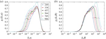
With the inclusion of the effects of spatial intermittency, the appropriate spectral form of (1.5) when compensated becomes
 $$\begin{eqnarray}\displaystyle g_{1}(k_{1}{\it\eta})=(k_{1}R)^{{\it\mu}/9}f_{1}(k_{1}{\it\eta}),\quad g_{2}(k_{1}R)=(k_{1}R)^{{\it\mu}/9}f_{2}(k_{1}R), & & \displaystyle\end{eqnarray}$$
for, respectively, inner and outer scalings. These are equivalent to the K41 scalings of (3.1) and (3.2) (see Monin & Yaglom Reference Monin and Yaglom1975, p. 642, for example). Figure 4 shows spectra in this form,
 ${\it\mu}=0.5$
. Comparison of figures 2(a) and 4(a) shows that the degree of collapse with inner scaling is generally worse with the K62 compensation. Similarly, comparison of figures 2(b) and 4(b) shows that the degree of collapse is approximately the same, but the slope on the inertial range has increased.


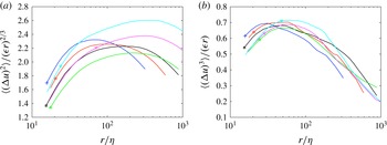
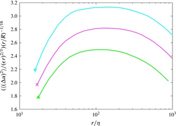
The nature of the incomplete similarity illustrated by figure 4(a,b) may be further investigated by examining the second-order structure function (the third-order moments are unchanged). Figure 5 shows the second-order structure function corrected for the effects of large-scale intermittency using (1.2) with
 $n=2$
and
 ${\it\mu}=0.5$
. Although it shows a broad plateau (its width increasing with Reynolds number),
 $C_{2}$
shows an even greater Reynolds-number dependence than the corresponding K41 scaling in figure 3(a).
4. Discussion
We believe the results of figure 1 to be our most far reaching. It is important to note that the non-dimensionalisation of
 ${\it\epsilon}$
here uses the imposed scales
 $u_{{\it\tau}}$
and
 $R$
, rather than the more usual non-dimensionalisation using ‘intrinsic’ scales, such as the root mean square of the fluctuating velocity
 $u^{\prime }=\surd \overline{u^{2}}$
, and the dissipation length scale
 $L_{{\it\epsilon}}=u^{\prime 3}/{\it\epsilon}$
(see e.g. Sreenivasan Reference Sreenivasan1995; Ishihara et al.
Reference Ishihara, Gotoh and Kaneda2009). Trivially, one could write
 $B={\it\epsilon}/(u^{\prime 3}/L_{{\it\epsilon}})\equiv 1$
. Therefore the use of imposed scales in figure 1 describes non-self-similar effects of the boundary conditions on the spectral flux, here caused by large-scale transport.
Hultmark et al. (Reference Hultmark, Vallikivi, Bailey and Smits2012) show that, at the centreline,
 $u^{\prime +}=u^{\prime }/u_{{\it\tau}}$
is more or less constant with Reynolds number. Writing
 $$\begin{eqnarray}A=\frac{{\it\epsilon}}{u_{{\it\tau}}^{3}/R}=\frac{u^{\prime 3}/L_{{\it\epsilon}}}{u_{{\it\tau}}^{3}/R}\sim \frac{R}{L_{{\it\epsilon}}},\end{eqnarray}$$
the slight increase of
 $A$
with
 $Re_{{\it\lambda}}$
can be interpreted as the influence of the outer boundary condition on
 ${\it\epsilon}$
: by using the locally isotropic estimate,
 ${\it\epsilon}=15{\it\nu}\overline{(\partial u/\partial x)^{2}}\sim u_{{\it\tau}}^{3}/R$
,
 $$\begin{eqnarray}A=\frac{{\it\epsilon}}{u_{{\it\tau}}^{3}/R}=15\frac{R^{+}}{Re_{{\it\lambda}}^{2}}\sim 1.\end{eqnarray}$$
Hence (4.2) does not fully account for the effects of the outer boundary condition in spite of assuming
 ${\it\epsilon}\sim u_{{\it\tau}}^{3}/R$
. This important result is not the same as that shown, for example, by Sreenivasan (Reference Sreenivasan1995), in which the influence of the large scales appears as
 $C_{{\it\epsilon}}\equiv A$
decreasing with
 $Re_{{\it\lambda}}$
. Vassilicos (Reference Vassilicos2015) has suggested that, for turbulence grids, ‘inlet,
 $I$
’ or global effects may be accounted for by
 $C_{{\it\epsilon}}\sim Re_{I}^{m}/Re_{L}^{n}$
with
 $m\approx 1\approx n$
, where the subscript
 $L$
denotes a local Reynolds number. This can be adapted for the present case by inspection so that (4.2) gives
 $A$
increasing with
 $Re_{{\it\lambda}}$
. Note that the formulation of K62 is such that
 ${\it\epsilon}$
retains its self-similar form, and therefore it cannot describe the above effects.
Second-order (
 $n=2$
) moments, compensated for K62, (1.2), with
 ${\it\mu}=0.5$
.

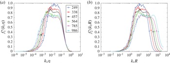
The lack of a universal description of the inertial subrange suggests that an empirical approach might prove beneficial. Mydlarski & Warhaft (Reference Mydlarski and Warhaft1996) present a modified similarity form in which (3.1) becomes
 $$\begin{eqnarray}f_{1}^{\ast }(k_{1}{\it\eta})={\it\epsilon}^{-2/3}k_{1}^{5/3}(k_{1}{\it\eta})^{-(5/3)+n_{1}}{\it\phi}_{11}(k_{1})=\frac{(k_{1}{\it\eta})^{n_{1}}}{v_{{\it\epsilon}}^{2}}{\it\phi}_{11}(k_{1}{\it\eta}),\end{eqnarray}$$
where
 $n_{1}$
is determined empirically using grid turbulence as
 $$\begin{eqnarray}n_{1}={\textstyle \frac{5}{3}}(1-3.15Re_{{\it\lambda}}^{-2/3})\end{eqnarray}$$
in the range
 $50\leqslant Re_{{\it\lambda}}\leqslant 473$
. At sufficiently large Reynolds number,
 $f_{1}^{\ast }(k_{1}{\it\eta})\rightarrow C$
. With outer scaling (4.3) becomes
 $$\begin{eqnarray}f_{2}^{\ast }(k_{1}R)=A^{-2/3}\frac{(k_{1}R)^{n_{1}}}{u_{{\it\tau}}^{2}}\left(\frac{{\it\eta}}{R}\right)^{-(5/3)+n_{1}}{\it\phi}_{11}(k_{1}R),\end{eqnarray}$$
where, at large Reynolds number,
 $f_{2}^{\ast }(k_{1}R)\rightarrow C$
also. Here the constant
 ${\it\mu}$
of K62, (1.3), is replaced by the empirical function, (4.4).
Figure 6(a,b) shows spectra with inner and outer scalings indicated by (4.3) and (4.5) respectively: there are identifiable plateaux with both inner and outer scaling at the three highest Reynolds numbers, with an ordinate value of about
 $0.73$
, very close to the Mydlarski & Warhaft (Reference Mydlarski and Warhaft1996) value. However, this is not the self-similar value of about
 $0.55$
(see figure 2) and the difference is presumably due to the empirical function.


Second-order (
 $n=2$
) moments, compensated using Mydlarski & Warhaft (Reference Mydlarski and Warhaft1996) function (4.4). Same data as figure 5.

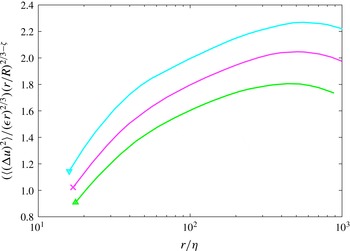
The second-order structure function (the Fourier transform pair of (4.3)) may be written
 $$\begin{eqnarray}\frac{\langle ({\rm\Delta}u)^{2}\rangle }{({\it\epsilon}r)^{2/3}}=C_{2}\left(\frac{r}{R}\right)^{{\it\zeta}-(2/3)},\end{eqnarray}$$
where
 ${\it\zeta}=(2/3)(1-7.88Re_{{\it\lambda}}^{-2/3})$
, from (4.4). Figure 7 shows the second-order moment premultiplied to preserve the value of the constant
 $C_{2}$
. In comparison to the K62 scaling in figure 5, the collapse is rather better. However, there is no clear plateau. The lack of collapse in both figures 6 and 7 is perhaps not unexpected, given that the empirical information derives from decaying turbulence, rather than that at the centreline of fully developed pipe flow.
5. Conclusions
A dual-space spectral description of energy flux has been provided for the centreline of turbulent pipe flow up to
 $Re_{{\it\lambda}}\approx 1000$
. Direct effects of viscosity appear at the centreline although the correction of the ‘
 $4/5$
ths’ constant for finite Reynolds number by Lundgren (Reference Lundgren2002) yields values of
 $0.80\pm 0.01$
. It should be pointed out, however, that Lundgren’s theory is developed for decaying isotropic turbulence. A greater challenge is presented by the effects of transport, even at the centreline – Danaila et al. (Reference Danaila, Anselmat, Zhou and Antonia2001) (see also Antonia & Burattini Reference Antonia and Burattini2006) have investigated the need for corrections to (1.7) at low Reynolds numbers to account for the effects of the large scales. There is no clear plateau in the third-order moment even when corrected for the effects of boundary conditions as described by K62, or empirically. Both viscous and turbulent transport contribute to a non-conservative spectral flux, the effect of which is clearly evident both in the corresponding spectra and in the dimensionless dissipation rate. Turbulent transport, which is finite at the centreline (left-hand side of (1.6)), is clearly the dominant mechanism in determining global effects on spectral flux. Moreover, these effects cannot be described well by Kolmogorov (Reference Kolmogorov1962) in which
 ${\it\epsilon}$
retains its self-similar form.
Future work involves an investigation of the effects of mean shear, and examination of long data records to investigate high-wavenumber intermittency.
Acknowledgements
This work was supported by the Office of Naval Research grant no. N00014-13-1-0174. M.V. is grateful for additional financial support from Estonian Students Fund, Zonta International, as well as several Princeton alumni fellowships. J.F.M. is indebted to the Engineering and Physical Sciences Research Council (grants GR/M64536/01 and GR/R48193/01), an Engineering Foresight Award (Royal Academy of Engineering, England), and the Leverhulme Trust (grant F/07058/H) for financial support.