

1 Introduction
Cavitation bubbles produce fast liquid jets when they collapse non-spherically in the vicinity of a solid boundary (Benjamin & Ellis Reference Benjamin and Ellis1966; Tomita & Shima Reference Tomita and Shima1986; Blake & Gibson Reference Blake and Gibson1987). These jets impacting on the solid boundary may be unwanted because they can damage the boundary (Tomita & Shima Reference Tomita and Shima1986; Philipp & Lauterborn Reference Philipp and Lauterborn1998), or may clean the boundary (Ohl et al. Reference Ohl, Arora, Dijkink, Janve and Lohse2006a; Kim et al. Reference Kim, Kim, Choi and Kim2009; Gonzalez-Avila et al. Reference Gonzalez-Avila, Huang, Quinto-Su, Wu and Ohl2011a), or may deliver drugs into cells (Prentice et al. Reference Prentice, Cuschieri, Dholakia, Prausnitz and Campbell2005; Ohl et al. Reference Ohl, Arora, Ikink, De Jong, Versluis, Delius and Lohse2006b; Le Gac et al. Reference Le Gac, Zwaan, van den Berg and Ohl2007) by the shear force from the accompanying radial spreading flow.
The bubble and the induced jet dynamics near a single solid boundary have been studied in great detail over the last five decades (Plesset & Chapman Reference Plesset and Chapman1971; Lauterborn & Bolle Reference Lauterborn and Bolle1975; Zhang, Duncan & Chahine Reference Zhang, Duncan and Chahine1993; Supponen et al. Reference Supponen, Obreschkow, Tinguely, Kobel, Dorsaz and Farhat2016). A much less explored configuration is that of a narrow gap, a configuration that is attracting increasing attention in cleaning (Gonzalez-Avila et al. Reference Gonzalez-Avila, van Blokland, Zeng and Ohl2018), electrical discharge machining (Shervani-Tabar, Abdullah & Shabgard Reference Shervani-Tabar, Abdullah and Shabgard2006) and biological applications (Hsiao et al. Reference Hsiao, Choi, Singh, Chahine, Hay, Ilinskii, Zabolotskaya, Hamilton, Sankin and Yuan2013; Yuan, Yang & Zhong Reference Yuan, Yang and Zhong2015; Mohammadzadeh, Li & Ohl Reference Mohammadzadeh, Li and Ohl2017). With the constriction of an additional solid boundary, a bubble oscillating inside a narrow gap with two rigid walls experiences even richer dynamics. The bubble may split into two daughter bubbles with two jets impacting on both walls when the gap is sufficiently small and the bubble is nucleated near the gap centre (Chahine Reference Chahine1982; Kucherenko & Shamko Reference Kucherenko and Shamko1986; Ishida et al. Reference Ishida, Nuntadusit, Kimoto, Nakagawa and Yamamoto2001; Azam et al. Reference Azam, Karri, Ohl, Klaseboer and Khoo2013; Ogasawara et al. Reference Ogasawara, Tsubota, Seki, Shigaki and Takahira2015). This behaviour has been reproduced by simulations using the boundary element method (Zhang et al. Reference Zhang, Ni, Song and Yao2010) and volume of fluid (VoF) method with a finite volume method framework (Han et al. Reference Han, Zhu, Guo, Liu and Ni2018). For a bubble created very close to one wall in a gap with a height comparable to the bubble’s maximum radius, it may translate to and induce a jet impacting on the distant wall during collapse. This feature was likely first observed by Gonzalez-Avila et al. (Reference Gonzalez-Avila, Klaseboer, Khoo and Ohl2011b) and reproduced by Quah et al. (Reference Quah, Karri, Ohl, Klaseboer and Khoo2018). Yet a thorough explanation is lacking. In a wider gap, an off-centre nucleated bubble acquires a quasi-conical shape and collapses onto the nearest wall (Kucherenko & Shamko Reference Kucherenko and Shamko1986; Gonzalez-Avila et al. Reference Gonzalez-Avila, Klaseboer, Khoo and Ohl2011b). These three distinct jetting dynamics were demonstrated by Gonzalez-Avila et al. (Reference Gonzalez-Avila, Klaseboer, Khoo and Ohl2011b). There, the collapse scenario could be predicted from a dimensionless gap height, which is the gap height normalized by the maximum horizontal bubble radius. However, the details at the final stage were not resolved due to spatial and temporal limitations in those experiments. Here the temporal resolution is considerably increased and the simulations now include viscous effects. Additionally the location of bubble nucleation is a parameter and its effect is reported.
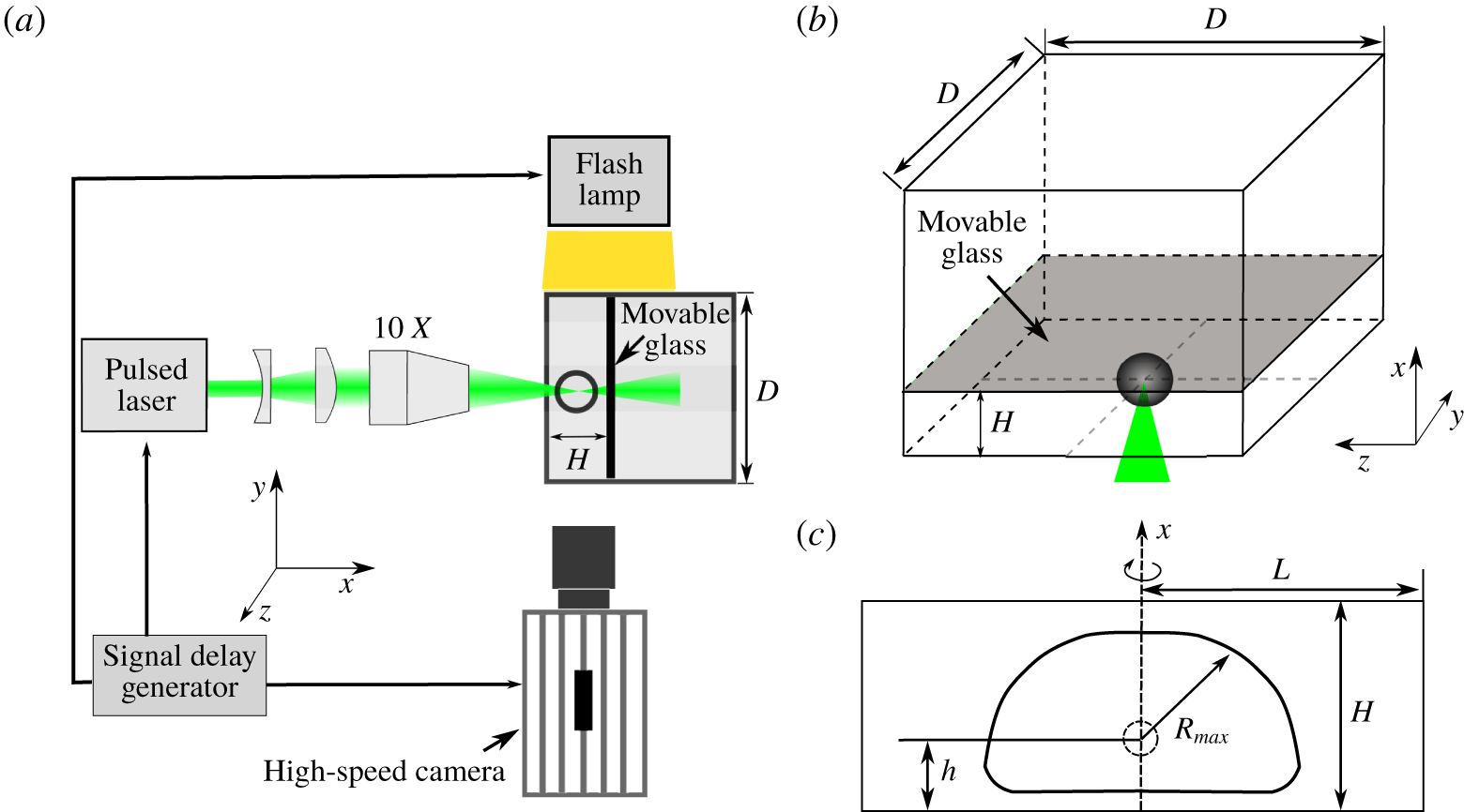
(a) Experimental set-up (top view). (b) Three-dimensional sketch of the geometry: the bubble is nucleated at the centre of the  $yz$ plane. (c) Sketch of the problem and parameters. The small circle at the axis is the nucleated bubble; the hat-shaped curve depicts the bubble outline at maximum expansion.

Simulation is becoming an important tool for resolving and understanding the experimentally observed fast dynamics on microscopic scales particularly during splitting and jetting of bubbles. Previously, many simulations of single and few cavitation bubbles were based on the numerically efficient boundary element method (Ishida et al. Reference Ishida, Nuntadusit, Kimoto, Nakagawa and Yamamoto2001; Shervani-Tabar et al. Reference Shervani-Tabar, Abdullah and Shabgard2006; Zhang et al. Reference Zhang, Ni, Song and Yao2010; Gonzalez-Avila et al. Reference Gonzalez-Avila, Klaseboer, Khoo and Ohl2011b; Hsiao et al. Reference Hsiao, Choi, Singh, Chahine, Hay, Ilinskii, Zabolotskaya, Hamilton, Sankin and Yuan2013), which is able to predict the splitting of a bubble and its conical shape while neglecting viscosity on the walls. Eventually, viscosity becomes important in the unsteady boundary layer that affects the bubble interface once it is close to the wall. Viscosity had been considered in an earlier work dealing with the bubble oscillations in a very narrow gap where Mohammadzadeh et al. (Reference Mohammadzadeh, Li and Ohl2017) used a commercial VoF solver to study the shear flow induced by a pancake-shaped bubble oscillating from the centre of the gap. They found boundary layer separation even for non-jetting cavitation bubbles. This was due to an adverse pressure gradient and strong shear at the crossover region between the boundary layer and the liquid bulk. Han et al. (Reference Han, Zhu, Guo, Liu and Ni2018) simulated a smaller cavitation bubble between two parallel solid plates using OpenFOAM. Here, the bubble creates wall-normal and annular jets and eventually splits. Their work focused on a few cases where the bubble position with respect to the wall is varied. Gonzalez-Avila et al. (Reference Gonzalez-Avila, van Blokland, Zeng and Ohl2018, Reference Gonzalez-Avila, van Blokland, Zeng and Ohl2020) conducted a systematic study of the channel height, where the bubble position was fixed close to one boundary. That latter study used a compressible VoF solver again with the open source package OpenFOAM. Simulation and experiments show excellent agreement for the bubble shape, centre of mass motion, jet direction and jet speed.
The present study connects two previous works of Han et al. (Reference Han, Zhu, Guo, Liu and Ni2018) and Gonzalez-Avila et al. (Reference Gonzalez-Avila, van Blokland, Zeng and Ohl2020) in a parametric study that accounts for the effect of gap height and bubble position within the gap. It does not repeat previous work on mostly planar bubbles in very narrow gaps such as that of Zwaan et al. (Reference Zwaan, Le Gac, Tsuji and Ohl2007) and Quinto-Su & Ohl (Reference Quinto-Su and Ohl2009). Moreover, we account for a parameter that has not received much attention, namely the length of the gap. In the present work we start with a description of the experimental and numerical methodologies, then present the results in § 3 and a discussion in § 4.
2 Methodology
Individual bubbles are generated by focusing a laser pulse into a narrow gap whose height  $H$ is adjustable. Figure 1(a) shows the top view of the experimental set-up and figure 1(b) a three-dimensional view from the camera side. To nucleate the bubble, a Q-switched Nd:YAG laser pulse (532 nm wavelength, 6 ns duration) is expanded and collimated with a combination of a plano-concave and a plano-convex lens before it is focused into the gap with a 10
 $\times$ microscope objective (Olympus UPlanFL N10X 0.30 NA). The narrow gap is formed by two plane boundaries made of glass, all other boundaries being made of transparent acrylic surfaces. The position of the bubble nucleation site is controlled by moving the whole gap along the laser beam direction to adjust the parameter
 $h$ as shown in figure 1(c). A high-speed camera (Shimadzu Hypervision HPV-2) records the bubble dynamics from the side at 500 000 frames per second. The scene is recorded with mildly diffused light from a flash lamp. The resolution is
 $18~\unicode[STIX]{x03BC}\text{m}$ per pixel. The camera, pulsed laser and flash are synchronized with a delay generator (Quantum, 9520 series).
As shown in figure 1(b), the flow domain in the experiment is a cuboid with a volume of  $H\times D\times D$ (here
 $D=10~\text{mm}$ is the length of the square base of the cuvette, and
 $H$ is varied between
 $0.6$ and
 $2.7~\text{mm}$). The movable glass and the glass fixed at the bottom form the gap. The remaining boundaries are the two rigid walls of the cuvette (front and back walls along the
 $y$ direction) and two submerged boundaries (left and right boundaries along the
 $z$ direction). In each test we ensure the bubble is nucleated at the centre of the
 $yz$ plane. All other boundaries in the
 $xy$ planes and
 $xz$ planes are sufficiently far from the bubble to limit their effect on the bubble dynamics. All experimental and simulation results show the bubble in the
 $xz$ plane (see figure 1c).
In the simulations, the geometry is further simplified to an axisymmetric domain, i.e. a cylinder oriented in the  $x$ direction with a radius of
 $L$ (
 $=D/2$) and height
 $H$. The simulations start with a spherical bubble with an initial radius
 $R_{0}$ at a uniform internal over-pressure
 $P_{0}$ positioned at a distance
 $h$ to the lower boundary of a submerged liquid gap. The bubble then expands to a maximum spherical equivalent radius
 $R_{max}$. For a bubble near a single rigid boundary, its dynamics can be characterized by the stand-off distance
 $\unicode[STIX]{x1D6FE}=h/R_{max}$ (Plesset & Chapman Reference Plesset and Chapman1971; Lauterborn & Bolle Reference Lauterborn and Bolle1975; Blake & Gibson Reference Blake and Gibson1987). For a bubble inside a gap we use the normalized off-centre distance
 $\unicode[STIX]{x1D701}=(H/2-h)/R_{max}$. The bubble collapse dynamics is also affected by the normalized gap height
 $\unicode[STIX]{x1D702}=H/R_{max}$ and the normalized gap radius
 $l=L/R_{max}$, which together describe the geometric confinement. The stand-off parameter
 $\unicode[STIX]{x1D6FE}$ refers always to the closest wall and is related to
 $\unicode[STIX]{x1D701}$ and
 $\unicode[STIX]{x1D702}$ by
 $\unicode[STIX]{x1D6FE}=h/R_{max}=\unicode[STIX]{x1D702}/2-\unicode[STIX]{x1D701}$.
To simulate the bubble dynamics and induced liquid jet, we assume the bubble as non-condensable gas following a polytropic equation of state and consider the surrounding liquid as a Tait-compressible liquid (Macdonald Reference Macdonald1969), similar to Koukouvinis et al. (Reference Koukouvinis, Strotos, Zeng, Gonzalez-Avila, Theodorakakos, Gavaises and Ohl2018). The nonlinear compressibility is computed as  $\unicode[STIX]{x1D713}=D\unicode[STIX]{x1D70C}/Dp$ based on the equation of state, where
 $\unicode[STIX]{x1D70C}$ and
 $p$ are the density and pressure, respectively. Using the VoF method for a compressible two-phase flow problem, the volume fraction of the liquid phase
 $\unicode[STIX]{x1D6FC}$ is solved with the transport equation (Miller et al. Reference Miller, Jasak, Boger, Paterson and Nedungadi2013; Koch et al. Reference Koch, Lechner, Reuter, Köhler, Mettin and Lauterborn2016; Zeng et al. Reference Zeng, Gonzalez-Avila, Ten Voorde and Ohl2018b):
 $$\begin{eqnarray}\frac{\unicode[STIX]{x2202}\unicode[STIX]{x1D6FC}}{\unicode[STIX]{x2202}t}+\unicode[STIX]{x1D735}\boldsymbol{\cdot }(\unicode[STIX]{x1D6FC}\boldsymbol{u})+\unicode[STIX]{x1D735}\boldsymbol{\cdot }(\unicode[STIX]{x1D6FC}(1-\unicode[STIX]{x1D6FC})\boldsymbol{U}_{\boldsymbol{r}})=\unicode[STIX]{x1D6FC}(1-\unicode[STIX]{x1D6FC})\left(\frac{\unicode[STIX]{x1D713}_{g}}{\unicode[STIX]{x1D70C}_{g}}-\frac{\unicode[STIX]{x1D713}_{l}}{\unicode[STIX]{x1D70C}_{l}}\right)\frac{\text{D}p}{\text{D}t}+\unicode[STIX]{x1D6FC}\unicode[STIX]{x1D735}\boldsymbol{\cdot }\boldsymbol{u},\end{eqnarray}$$
where  $\boldsymbol{u}$ is the velocity field,
 $t$ is time and subscripts
 $l$ and
 $g$ represent the liquid and gas phases, respectively. Here
 $\boldsymbol{U}_{\boldsymbol{r}}$ is the relative velocity between two phases and acts as an artificial compressible term ensuring a sharp interface (Rusche Reference Rusche2003).
The two phases are treated as compressible and immiscible Newtonian fluids. The thermal effect of the flow is mainly due to two mechanisms. They are the heat transfer between a collapsing hot bubble and nearby liquid (Beig, Aboulhasanzadeh & Johnsen Reference Beig, Aboulhasanzadeh and Johnsen2018) and liquid temperature rise through viscous dissipation by strong jet shearing on no-slip rigid surfaces (Kondo & Ando Reference Kondo and Ando2019). Yet both are negligible here since the small temperature increment and the short duration are not possible for an effective mass transfer. Neglecting heat and mass transfer, the governing equations for the flow are the Navier–Stokes equations:
 $$\begin{eqnarray}\displaystyle & \displaystyle \frac{\unicode[STIX]{x2202}\unicode[STIX]{x1D70C}}{\unicode[STIX]{x2202}t}+\unicode[STIX]{x1D735}\boldsymbol{\cdot }(\unicode[STIX]{x1D70C}\boldsymbol{u})=0, & \displaystyle\end{eqnarray}$$
 $$\begin{eqnarray}\displaystyle & \displaystyle \frac{\unicode[STIX]{x2202}\unicode[STIX]{x1D70C}\boldsymbol{u}}{\unicode[STIX]{x2202}t}+\unicode[STIX]{x1D735}\boldsymbol{\cdot }(\unicode[STIX]{x1D70C}\boldsymbol{u}\boldsymbol{u})=-\unicode[STIX]{x1D735}p+\unicode[STIX]{x1D735}\boldsymbol{\cdot }\unicode[STIX]{x1D749}+\boldsymbol{f}_{\unicode[STIX]{x1D739}}, & \displaystyle\end{eqnarray}$$
where  $\unicode[STIX]{x1D749}$ is the viscous stress tensor which is calculated as
 $\unicode[STIX]{x1D749}=\unicode[STIX]{x1D707}[\unicode[STIX]{x1D735}\boldsymbol{u}+\unicode[STIX]{x1D735}\boldsymbol{u}^{\text{T}}-\frac{2}{3}(\unicode[STIX]{x1D735}\boldsymbol{\cdot }\boldsymbol{u})\unicode[STIX]{x1D644}]$,
 $\unicode[STIX]{x1D707}$ and
 $\unicode[STIX]{x1D644}$ are the dynamic viscosity and the identity tensor, respectively, and
 $\boldsymbol{f}_{\unicode[STIX]{x1D739}}$ is the source term due to surface tension which is modelled according to the so-called continuous-surface-force method (Brackbill, Kothe & Zemach Reference Brackbill, Kothe and Zemach1992).
The compressible Navier–Stokes equations and the transport equation (2.1) are solved together in an axisymmetric domain to reproduce the flow field in OpenFOAM (Weller et al. Reference Weller, Tabor, Jasak and Fureby1998). The boundary conditions are no slip for both walls, and the ambient pressure  $P_{\infty }=101\,325~\text{Pa}$ at the exit of the gap. Compressibility of both gas and liquid phases, surface tension and viscosity are included in the model. In particular, the viscosity is essential for resolving the flow in the vicinity of the boundary layer. A locally and recursively refined mesh is used, which has a cell size of approximately
 $1.5~\unicode[STIX]{x03BC}\text{m}$ wide in the area where the bubble is located. In each simulation, the whole gap of the domain is modelled as the gap length is an important parameter for the bubble dynamics. The images presented below are showing only the central part with the bubble present. More details of the simulations can be found in Zeng et al. (Reference Zeng, Gonzalez-Avila, Dijkink, Koukouvinis, Gavaises and Ohl2018a,Reference Zeng, Gonzalez-Avila, Ten Voorde and Ohlb).
3 Results
3.1 Bubble dynamics
In this section, we present selected scenarios of the bubble dynamics from experiment and simulation and analyse the flow during jet formation. In both experiments and simulations the distance  $D$ is fixed to
 $D=2\times L=10~\text{mm}$ while the height of the gap and the bubble position are varied. The explosive growth of the cavitation bubble is induced in the simulations with a high-pressure spherical gas pocket at
 $t=0$ with an initial bubble radius
 $R_{0}=50~\unicode[STIX]{x03BC}\text{m}$. The only free parameter in the simulation is the initial pressure of the bubble which is adjusted to meet the experimental period of growth and collapse.
We now discuss three cases that lead to the three distinct jetting phenomena: transferred jet, double jet and directed jet.
3.1.1 Transferred jet
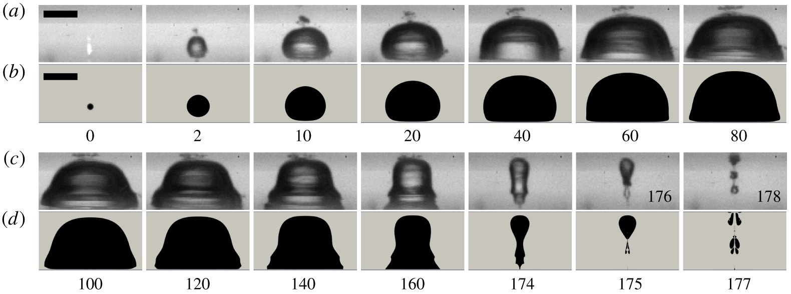
Figure 2 compares selected frames of an experimental run with the simulation with  $H=840~\unicode[STIX]{x03BC}\text{m}$ and
 $h=228~\unicode[STIX]{x03BC}\text{m}$. Note that the images from the experiment are photographic projections while the simulation result shows the cut plane of the fluid domain revealing flows within the bubble that are difficult to see in the experiment. The top and bottom of each frame are the positions of the rigid boundaries forming the gap. In the experiment, the nucleation volume is not perfectly spherical but elongated in the vertical direction. This may result in an ellipsoidal bubble in the very early stage or even two bubbles that quickly merge. We find that this non-spherical initial condition has little effect on the later bubble dynamics which is dominated by the nearby boundaries.
Configuration resulting in a transferred jet:  $H=840~\unicode[STIX]{x03BC}\text{m}$ and
 $h=228~\unicode[STIX]{x03BC}\text{m}$. (a,c) In the experiment,
 $R_{max}=553\pm 18~\unicode[STIX]{x03BC}\text{m}$,
 $\unicode[STIX]{x1D702}=1.52\pm 0.06$ and
 $\unicode[STIX]{x1D701}=0.35\pm 0.03$. (b,d) In the simulation,
 $R_{max}=526~\unicode[STIX]{x03BC}\text{m}$,
 $\unicode[STIX]{x1D702}=1.60$,
 $\unicode[STIX]{x1D701}=0.37$ and the initial pressure
 $P_{0}=1000~\text{bar}$. The scale bar represents
 $500~\unicode[STIX]{x03BC}\text{m}$. Numbers below the frames indicate the time in microseconds.

We set the time of bubble nucleation to  $t=0$, that is, the time of firing the laser pulse (activation of the Q-switch) that creates the plasma. For the simulations, this complex laser–matter interaction is avoided and we start with a spherical bubble nucleus of radius
 $R_{0}=50~\unicode[STIX]{x03BC}\text{m}$ and an internal pressure of
 $p_{0}=1000~\text{bar}$. This results in an explosively expanding bubble whose lower bubble wall quickly flattens at
 $t=10~\unicode[STIX]{x03BC}\text{s}$. From then on the bubble grows sideways losing its spherical shape. At time
 $t\approx 100~\unicode[STIX]{x03BC}\text{s}$ the bubble obtains its maximum volume and a top-hat shape. The computed bubble has a slightly smaller maximum radius
 $R_{max}=526~\unicode[STIX]{x03BC}\text{m}$ as compared to the experimental bubble
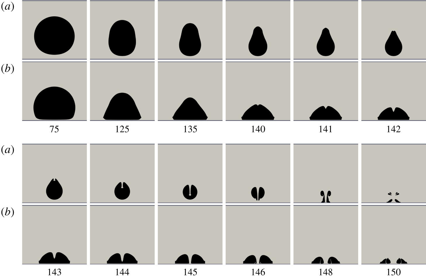
 $R_{max}=553\pm 18~\unicode[STIX]{x03BC}\text{m}$. Overall we obtain very good agreement of the bubble outline and timing between simulation and experiment for the expansion stage. In the vertical direction the bubble occupies almost the whole gap. The collapse dynamics results in a corrugated cylindrical shape at
 $t=160~\unicode[STIX]{x03BC}\text{s}$. We discuss below that this is caused by the unsteady boundary layers where the inflow and radial outflow compete.
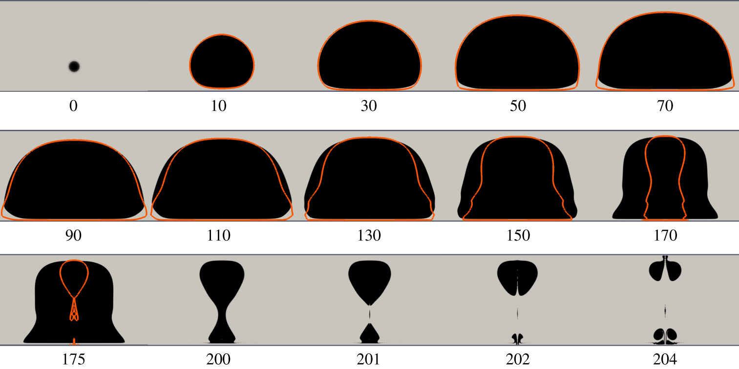
As a result, the lower part of the bubble shrinks first and the centre of gravity of the bubble translates upwards. A shrinking and translating bubble develops a jet in the direction of movement (Blake & Gibson Reference Blake and Gibson1987; Supponen et al. Reference Supponen, Obreschkow, Tinguely, Kobel, Dorsaz and Farhat2016), i.e. the jet impinges onto the upper boundary. Jets impacting on the opposite boundary of bubble generation are named transferred jets in this work. On a closer look we find the formation of two upward-pointing jets, one from the central cylindrical bubble formed between  $t=174~\unicode[STIX]{x03BC}\text{s}$ and
 $t=175~\unicode[STIX]{x03BC}\text{s}$. The cylindrical bubble splits and from this location a second transferred jet is formed that impacts onto the upper boundary. From the experiments we can estimate for this second jet a lower bound of the velocity of
 $210\pm 53~\text{m}~\text{s}^{-1}$, while the simulations give a value of
 $280~\text{m}~\text{s}^{-1}$. This complex experimental scenario of bubble splitting and translation of the fragments is faithfully reproduced in the simulations.
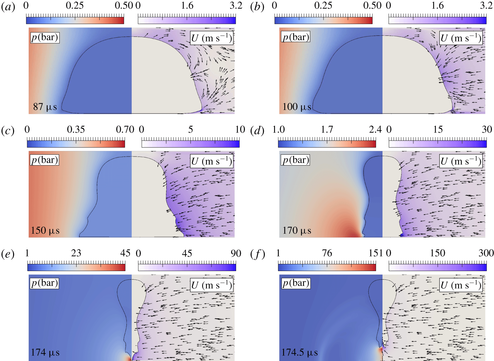
Pressure distribution (left part of each panel) and velocity field (right part of each panel) during jet formation for the case in figure 2. The arrows all have the same length and only indicate direction. The colour bars depict pressure and speed. Note that the range varies greatly in the panels.

While the temporal resolution of the experiment is limited by the exposure time and frame rate, the simulations offer the opportunity to carefully look at the flow field, here in particular during the jetting. Figure 3 depicts relevant pressure and flow fields on the left- and right-hand side of each panel, respectively. The pressure field is colour coded from low (blue) to high (red). The direction of the flow is indicated with arrows on the right-hand side of each panel of figure 3. The magnitude of the flow velocity is coded from low (white) to high (blue).
Already at the late stage of expansion  $(t=87~\unicode[STIX]{x03BC}\text{s})$, the liquid far from the bubble is accelerated back towards the axis of symmetry by the adverse pressure gradient. Moreover, at the same time the bubble is still expanding and pushing the nearby liquid outwards. Near the walls this expanding flow is deflected by the incoming flow, resulting in a downward flow from the upper wall and an upward flow from the lower wall. The downward flow and the upward flow collide and together with the incoming flow an annular jet flow towards the bubble’s centre is formed. This flow forms a dimpled annular ring on the bubble. The dimple serves as an initial perturbation and during the collapse develops into a ‘neck’ on the bubble (see the central part of the bubble in figure 3d–f). Now we look at the lower bubble wall from where the first jet is created. During the expansion, this part of the bubble flattens and a thin liquid film with a height of
 $5~\unicode[STIX]{x03BC}\text{m}$ is formed. The liquid inside the gap flows slowly outwards thereby lifting up the the edge and forming there a strongly curved interface, already visible at the lower edge at
 $t=87~\unicode[STIX]{x03BC}\text{s}$. At
 $t=100~\unicode[STIX]{x03BC}\text{s}$ this region has the highest pressure gradient accelerating the flow inwards first in this region before the flow flips direction further away from the lower boundary. Additionally, as the lower part of the bubble is only
 $5~\unicode[STIX]{x03BC}\text{m}$ away from the boundary, the fastest inflow is not occurring closest to the lower boundary but slightly above. The effect is visible at
 $t=174~\unicode[STIX]{x03BC}\text{s}$ where a small tip at the bottom of the bubble remains. The stagnation pressure that builds up from the inward flow (velocity of
 $90~\text{m}~\text{s}^{-1}$ at
 $t=174~\unicode[STIX]{x03BC}\text{s}$) towards the the axis of symmetry is eventually emitted as an acoustic wave (see figure 3f). Coming back to the early collapse stage at
 $t=100~\unicode[STIX]{x03BC}\text{s}$, the pressure gradient is weakest at the top of the bubble and stronger at the centre of the gap. This results in a vertical flow from the top to the centre where it meets the bulk flow moving inward (see figure 3b). This region of the bubble splits (see
 $t=175~\unicode[STIX]{x03BC}\text{s}$ in figure 2) shortly after the first upward-directed jet has developed.
3.1.2 Double jet
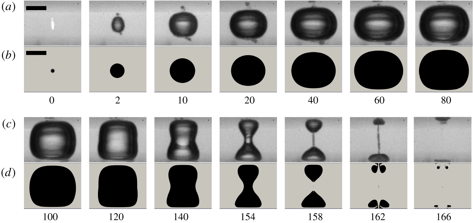
Figure 4 demonstrates the experimental and simulated dynamics for a bubble developing two jets on both walls. The bubble is created approximately at the centre of the gap with a width  $H=1100~\unicode[STIX]{x03BC}\text{m}$ and location
 $h=513~\unicode[STIX]{x03BC}\text{m}$. In the simulation, the bubble expands to a maximum radius
 $R_{max}=545~\unicode[STIX]{x03BC}\text{m}$ when starting with an initial pressure of 1100 bar, while in the experiment the bubble reaches a very similar maximum radius of
 $R_{max}=566\pm 18~\unicode[STIX]{x03BC}\text{m}$. The computed and experimental dimensionless parameters are
 $\unicode[STIX]{x1D702}=2.02$,
 $\unicode[STIX]{x1D701}=0.07$ and
 $\unicode[STIX]{x1D702}=1.94\pm 0.07$,
 $\unicode[STIX]{x1D701}=0.07\pm 0.03$, respectively. Again, we find convincing agreement between the calculated and simulated bubble shape that the essential fluid mechanics is covered in the simulation.
Configuration resulting in a double jet:  $H=1100~\unicode[STIX]{x03BC}\text{m}$ and
 $h=513~\unicode[STIX]{x03BC}\text{m}$. (a,c) In the experiment,
 $R_{max}=566\pm 18~\unicode[STIX]{x03BC}\text{m}$,
 $\unicode[STIX]{x1D702}=1.94\pm 0.07$ and
 $\unicode[STIX]{x1D701}=0.07\pm 0.03$. (b,d) In the simulations,
 $R_{max}=545~\unicode[STIX]{x03BC}\text{m}$,
 $\unicode[STIX]{x1D702}=2.02$,
 $\unicode[STIX]{x1D701}=0.07$ and the initial pressure
 $P_{0}=1100~\text{bar}$. The scale bar represents
 $500~\unicode[STIX]{x03BC}\text{m}$. Numbers below the frames indicate the time in microseconds.

Here, during the early expansion stage the bubble maintains a spherical shape. The upper and lower interface flatten slightly as they approach the walls due to the influence of the near-boundary liquid (Philipp & Lauterborn Reference Philipp and Lauterborn1998). The bubble acquires around maximum expansion a cylindrical shape, before an annular dimple becomes visible along the bubble’s equator (see  $t=120~\unicode[STIX]{x03BC}\text{s}$ in figure 4). This is an indication that during the early collapse stage the liquid is, as expected, fastest at the centre of the channel when the bubble is there. Then the dimple accelerates into an annular jet flowing inwards and eventually splits the bubble into two daughter bubbles once it impacts on the axis of symmetry (
 $t=158~\unicode[STIX]{x03BC}\text{s}$). There, a high-pressure region is formed that deflects the annular jet up and down creating two jets along the axis of symmetry. These two jets impact on the upper and lower boundary around
 $t=162~\unicode[STIX]{x03BC}\text{s}$. We name this case double jet where two counter-propagating jets are formed.
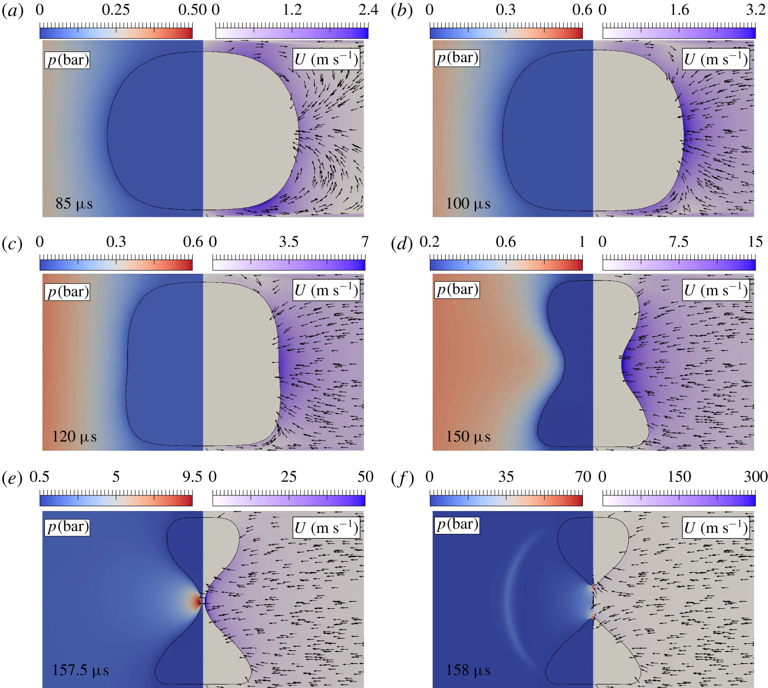
Pressure distribution (left part of each panel) and velocity field (right part of each panel) during jet formation for the case in figure 4. The arrows all have the same length and only indicate direction. The colour bars depict pressure and speed. Note that the range varies greatly in the panels.

Utilizing the simulations available, a detailed look at the double jet formation dynamics is portrayed in figure 5. Similar to figure 3, the flow from the walls is reflected by the incoming centre flow during the late expansion phase of the bubble (see figure 5a). Now are formed a rather symmetric pair of counter-rotating vortices near the upper and the lower walls. These two vortex rings of similar strengths collide and focus the annular jet on the central region of the bubble as shown in figure 5(b–e). Interestingly, the bubble parts close to the boundaries remain smooth as compared to the kinked shapes seen for the transferred jet in figures 2 and 3. For the earlier case the fastest flow was close to the lower boundary thus forming there a kink, while in the present case the near-boundary flow is accelerated smoothly upwards and downwards to the centre of the gap. There, the bubble is split by the closure of the annular jet. Just before  $t=157.5~\unicode[STIX]{x03BC}\text{s}$ a high-pressure region is formed and emitted into the liquid as a spherical wave, as seen at
 $t=158~\unicode[STIX]{x03BC}\text{s}$. Also, at this time the two jets emerging from this region become visible.
3.1.3 Directed jet
A third kind of bubble dynamics is observed by keeping the previous bubble size from the double jet constant,  $\unicode[STIX]{x1D702}=\text{const.}$, and moving the bubble nucleation point closer to the boundary, i.e. increasing
 $\unicode[STIX]{x1D701}$. The result of this parameter change is shown in figure 6 with
 $H=1055~\unicode[STIX]{x03BC}\text{m}$ and
 $h=295~\unicode[STIX]{x03BC}\text{m}$. The bubble reaches in the experiment a maximum radius
 $R_{max}=536\pm 18~\unicode[STIX]{x03BC}\text{m}$ (
 $\unicode[STIX]{x1D702}=1.97\pm 0.07$ and
 $\unicode[STIX]{x1D701}=0.43\pm 0.04$), while the computed bubble has a maximum radius
 $R_{max}=517~\unicode[STIX]{x03BC}\text{m}$ (
 $P_{0}=925~\text{bar}$,
 $\unicode[STIX]{x1D702}=2.04$ and
 $\unicode[STIX]{x1D701}=0.45$). Again, we see favourable agreement of the bubble shapes and timing between simulation and experiment.
Configuration resulting in a directed jet:  $H=1055~\unicode[STIX]{x03BC}\text{m}$ and
 $h=295~\unicode[STIX]{x03BC}\text{m}$. (a,c) In the experiment,
 $R_{max}=536\pm 18~\unicode[STIX]{x03BC}\text{m}$,
 $\unicode[STIX]{x1D702}=1.97\pm 0.07$ and
 $\unicode[STIX]{x1D701}=0.43\pm 0.04$. (b,d) In the simulation,
 $R_{max}=517~\unicode[STIX]{x03BC}\text{m}$,
 $\unicode[STIX]{x1D702}=2.04$,
 $\unicode[STIX]{x1D701}=0.45$ and the initial pressure
 $P_{0}=925~\text{bar}$. The scale bar represents
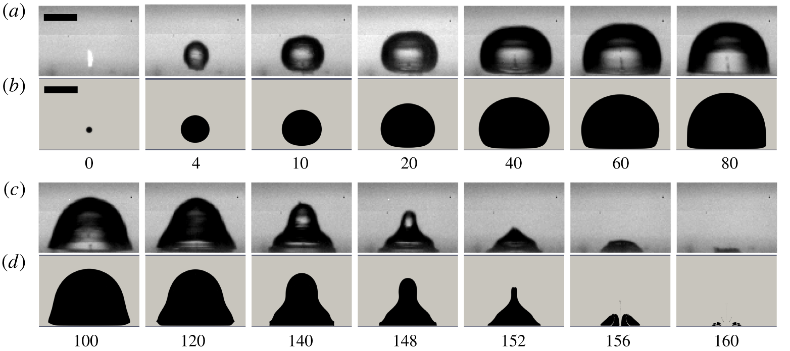
 $500~\unicode[STIX]{x03BC}\text{m}$. Numbers below the frames indicate the time in microseconds.

The bubble expands to a hemispherical shape at its maximum volume at time $t=80~\unicode[STIX]{x03BC}\text{s}$ with its bottom interface seemingly touching the lower boundary. From the simulation we find a liquid layer of about
 $5~\unicode[STIX]{x03BC}\text{m}$ in thickness between the bubble and the wall. The shrinkage of the bubble starts from the sides where the pressure gradient is strongest (see below). This incoming annular flow shapes the upper part of the bubble into a cylinder with a peculiar shape of its upper surface (see time
 $t=140~\unicode[STIX]{x03BC}\text{s}$). Once this cylinder has collapsed, a conical bubble shape is found at time
 $t=152~\unicode[STIX]{x03BC}\text{s}$ that was reported previously by Tomita & Shima (Reference Tomita and Shima1986) and Chahine (Reference Chahine1982). Interestingly, the annular and downward flows converge at the bubble’s apex at time
 $148~\unicode[STIX]{x03BC}\text{s}\leqslant t\leqslant 152~\unicode[STIX]{x03BC}\text{s}$ in figure 6, accelerating the jet onto the lower wall. The spatial and temporal resolution in the experiment unfortunately does not allow a good estimate of this fast process and we find a lower bound of
 $100~\text{m}~\text{s}^{-1}$ of the averaged velocity similar to the highest velocities reported by Philipp & Lauterborn (Reference Philipp and Lauterborn1998) for
 $\unicode[STIX]{x1D6FE}=0.4$. We name this case directed jet with a single jet directed onto the closest boundary.
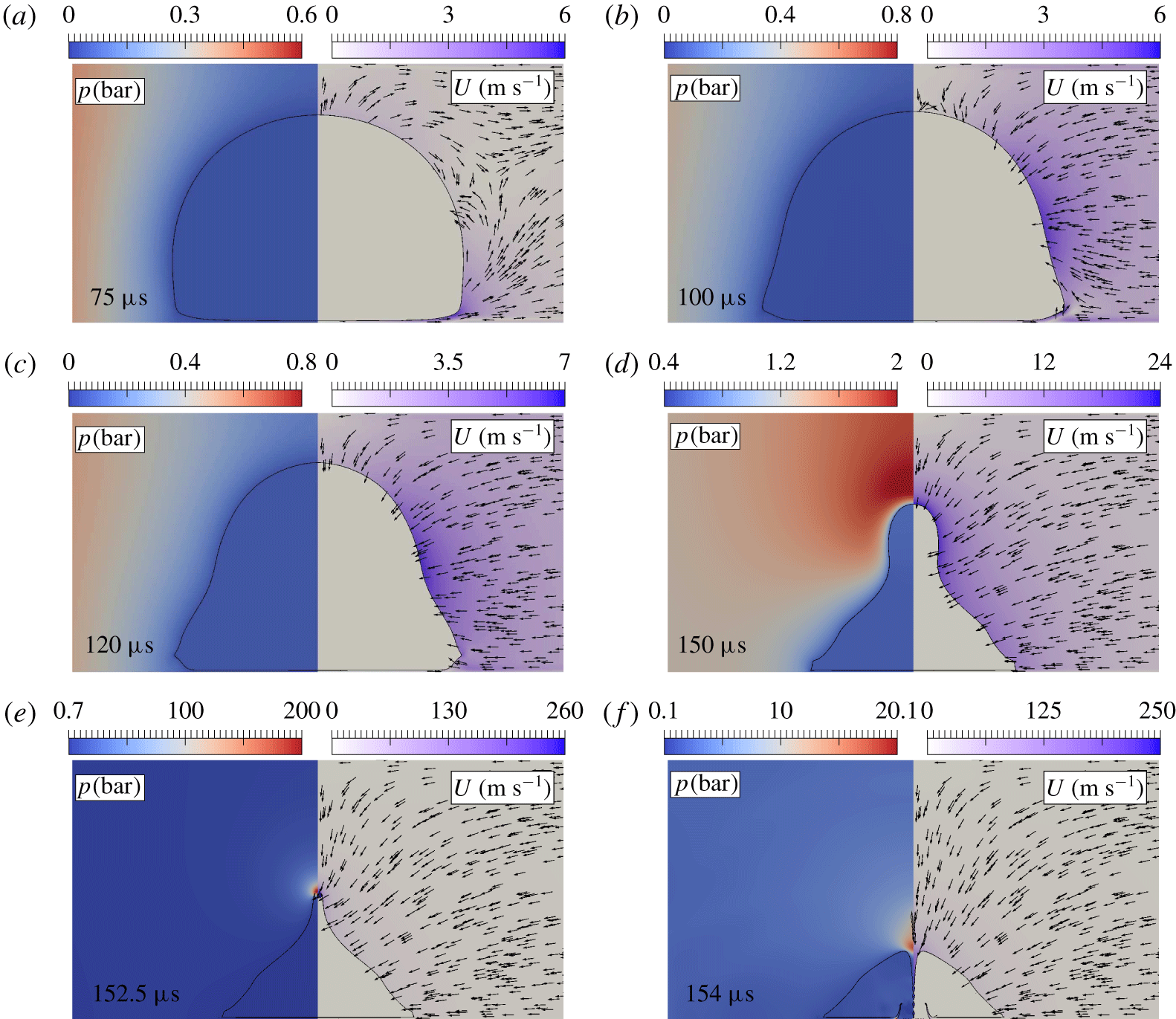
Pressure distribution (left part of each panel) and velocity field (right part of each panel) during jet formation for the case in figure 6. The arrows all have the same length and only indicate direction. The colour bars depict pressure and speed. Note that the range varies greatly in the panels.

Let us now have a closer look at the flow that drives the directed jet onto the wall in figure 7. At the late expansion stage  $t=75~\unicode[STIX]{x03BC}\text{s}$ we see the flow in the middle of the channel and close to the bubble is reflected as an inward flow focusing to the middle of the gap. There the bubble starts to shrink first from the sides (see time
 $t=100~\unicode[STIX]{x03BC}\text{s}$). During this early collapse the bubble shrinks fastest by the annular flow while the upper part moves inwards much slower (e.g. figure 7c). The top interface starts to move downwards with an appreciable velocity only after the bubble has obtained the elongated tip.
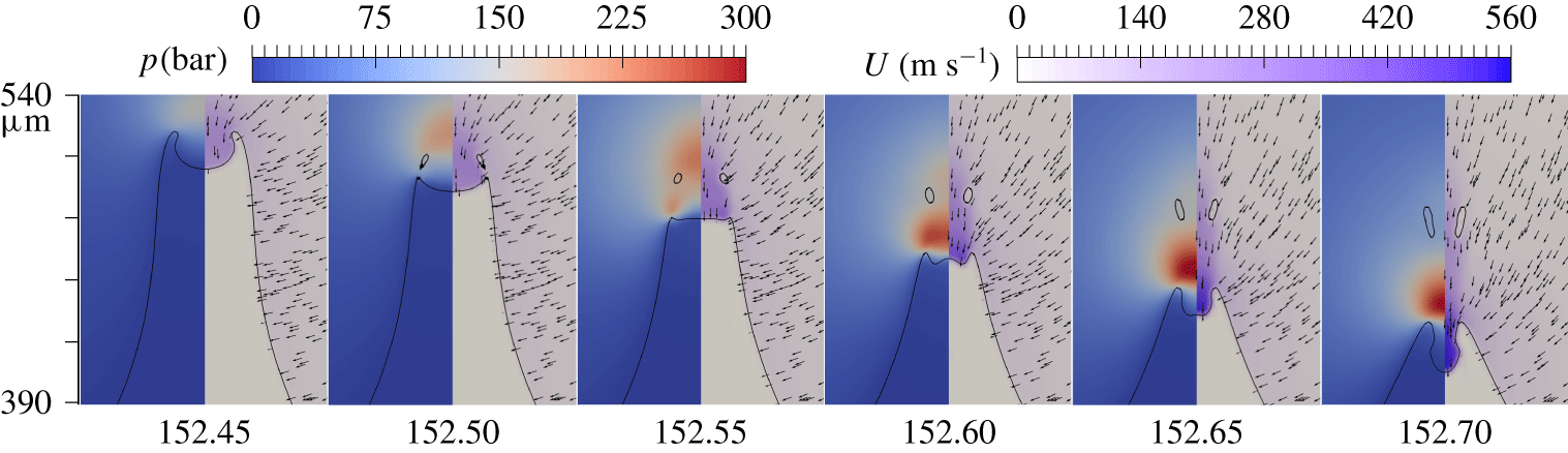
From this fast and high-pressure buildup at the top of the tip, an unexpected fast liquid jet emerges. This situation of a curved interface and rapid pressure increase seemingly resembles the situation of Antkowiak et al. (Reference Antkowiak, Bremond, Le Dizès and Villermaux2007), where a jet is formed by a pressure impulse acting on an inward-curved liquid–gas interface. In the present case the pressure buildup is caused by the convergent flow to the elongated apex (see figure 7e). By zooming spatially and temporally into this region, the rapid pressure buildup and the enormous gradients become evident. Figure 8 covers  $250~\text{ns}$ where the maximum pressure increases from approximately
 $\unicode[STIX]{x0394}p=100~\text{bar}$ to
 $\unicode[STIX]{x0394}p=300~\text{bar}$. The convergent flow towards the axis of symmetry confines the high-pressure region to a volume with a diameter of
 $\unicode[STIX]{x0394}d\approx 20~\unicode[STIX]{x03BC}\text{m}$ at
 $t=152.45~\unicode[STIX]{x03BC}\text{s}$; thus we expect an approximate average downward acceleration of
 $\text{D}u/\text{D}t=2\unicode[STIX]{x1D70C}^{-1}\unicode[STIX]{x0394}p/\unicode[STIX]{x0394}d\approx 2\times 10^{9}~\text{m}~\text{s}^{-2}$. Here, we use the average pressure during the acceleration
 $\unicode[STIX]{x0394}p=200~\text{bar}$. Assuming this acceleration acts for
 $\unicode[STIX]{x0394}t=200~\text{ns}$ (from
 $t=152.45~\unicode[STIX]{x03BC}\text{s}$ to
 $t=152.65~\unicode[STIX]{x03BC}\text{s}$), we expect an increase in velocity of
 ${\approx}400~\text{m}~\text{s}^{-1}$. This high-pressure buildup explains the rapid increase of the downward velocity from
 ${\approx}160$ to
 $560~\text{m}~\text{s}^{-1}$ over that short time interval
 $\unicode[STIX]{x0394}t$. Antkowiak et al. (Reference Antkowiak, Bremond, Le Dizès and Villermaux2007) report jet formation where a linear pressure impulse gradient is disturbed by a curved interface resulting in a focused flow similar to a shaped charge effect (Birkhoff et al. Reference Birkhoff, MacDougall, Pugh and Taylor1948). The present configuration has some resemblance during the early stage (see figure 7d), where the liquid–gas interface is concave. When this shape converts into a focused flow (see time
 $t=152.45~\unicode[STIX]{x03BC}\text{m}$ in figure 8) the interface flattens (time
 $t=152.55~\unicode[STIX]{x03BC}\text{s}$) before it accelerates above
 $500~\text{m}~\text{s}^{-1}$. Thus in contrast to Antkowiak et al. (Reference Antkowiak, Bremond, Le Dizès and Villermaux2007) the important driving mechanism may not be the shaped charge effect but the large pressure gradients built up by the cylindrical convergent flow colliding with the downwards flow on the axis of symmetry. A similar convergent flow has been reported for bubbles collapsing very close to a single boundary by Lechner et al. (Reference Lechner, Lauterborn, Koch and Mettin2019) where even higher velocities were reported.
Zoom-in details of figure 7 of the tip development. The width of the image is  $120~\unicode[STIX]{x03BC}\text{m}$.

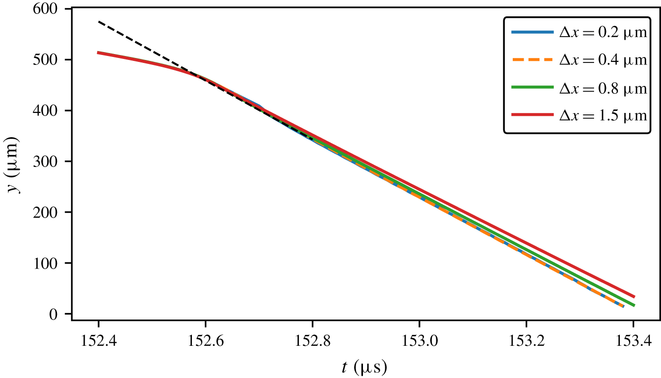
Movement of the jet tip under various mesh spacings during jet formation. The black dashed line represents a slope of  $580~\text{m}~\text{s}^{-1}$.

Figure 9 demonstrates this rapid acceleration of the initial jet flow and the convergence of the simulations. For the latter, the mesh was refined from  $1.5~\unicode[STIX]{x03BC}\text{m}$ to a grid spacing of
 $0.8$,
 $0.4$ and
 $0.2~\unicode[STIX]{x03BC}\text{m}$. The lines show the position of the jet tip on the axis of symmetry as a function of time. We find convergence and nearly indistinguishable lines for
 $0.4$ and
 $0.2~\unicode[STIX]{x03BC}\text{m}$. The tip movements for all mesh resolutions show a distinct transition of the slope at time
 $t\approx 152.6~\unicode[STIX]{x03BC}\text{s}$. Before time
 $t<152.6~\unicode[STIX]{x03BC}\text{s}$ the velocity is approximately
 $160~\text{m}~\text{s}^{-1}$ and accelerates to approximately
 $580~\text{m}~\text{s}^{-1}$ (dashed black line in figure 9) from
 $t>152.6~\unicode[STIX]{x03BC}\text{s}$. This fast thin jet occurs near the transition from the double jet to the directed jet, i.e. where the vertical flow velocity and the annular flow velocity are both rather high.
3.2 Pressure wave propagation
The creation of a bubble in a closed environment will result in a complex pattern of acoustic transients within a narrow gap due to the reflection of the waves at the sound hard walls and the soft boundary of the bubble. The time scale of the formation of these waves is of the order of  $H/c\approx 1~\unicode[STIX]{x03BC}\text{s}$, where
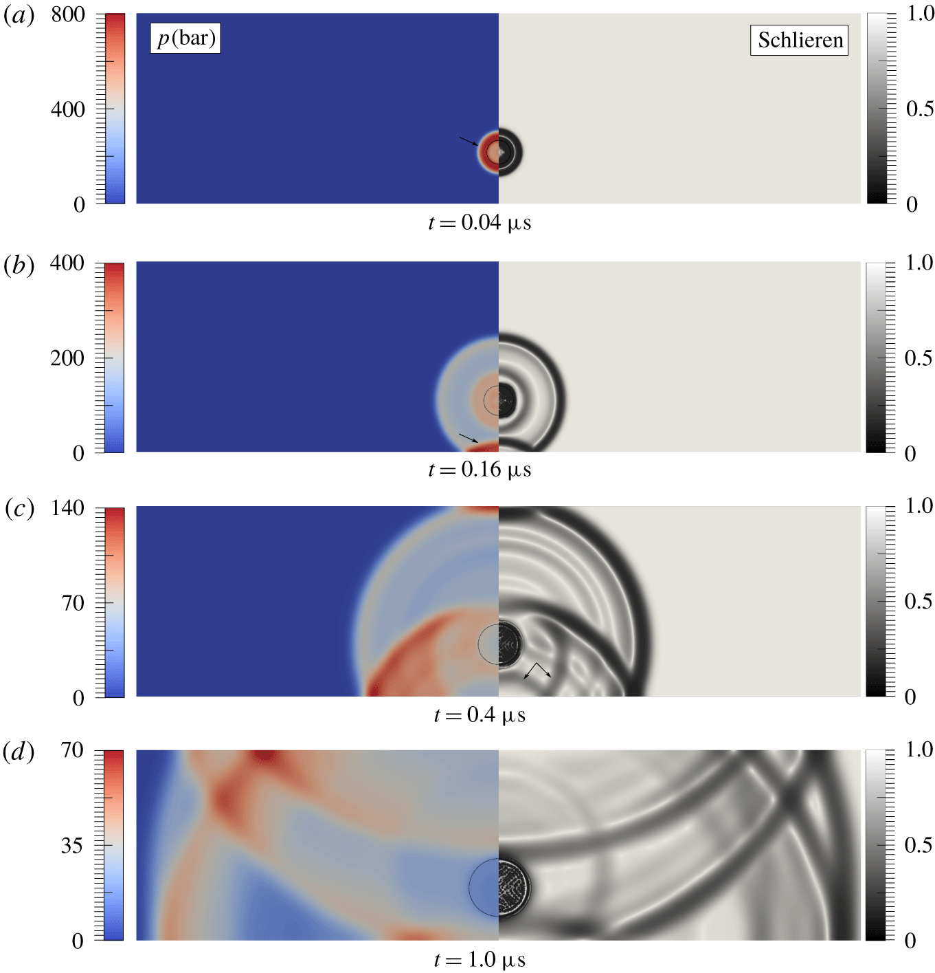
 $c=1500~\text{m}~\text{s}^{-1}$ is the speed of sound in water. Figure 10 zooms into the early expansion stage of the bubble shown in figure 2. The left part of each image in figure 10 depicts the colour-coded pressure while the right part is a numerically generated schlieren image. The schlieren value is calculated using the expression
 $\exp (-k|\unicode[STIX]{x1D735}\unicode[STIX]{x1D70C}|/\text{max}(|\unicode[STIX]{x1D735}\unicode[STIX]{x1D70C}|))$, where
 $k$ is an adjustable parameter.
Pressure wave propagation and numerical schlieren for the case shown in figure 2. Left: pressure field; right: numerical schlieren. The black lines in the left part represent the bubble interface. The top and bottom of the images coincide with the rigid boundaries. Image height is  $840~\unicode[STIX]{x03BC}\text{m}$ and the arrows refer to waves discussed in the text.

The explosive expansion of a bubble creates a spherical blast wave in the liquid bulk following its nucleation (see  $t=0.04~\unicode[STIX]{x03BC}\text{s}$). This wave is reflected acoustically hard back into the fluid domain (see
 $t=0.16~\unicode[STIX]{x03BC}\text{s}$). Later this wave is reflected as a rarefaction wave from the sound soft bubble and and refracted by the bubble in an upward-travelling transmitted wave (see the arrows at
 $t=0.4~\unicode[STIX]{x03BC}\text{s}$ in figure 10). Meanwhile, the upper part of the original shock wave reflects downwards from the upper wall and later interacts with the bubble and the lower wall. As a result, the original spherical wave divides into multiple waves. The interaction of these waves and the cavitation bubble results in a complex pressure distribution as visible in the schlieren pattern at time
 $t=1.0~\unicode[STIX]{x03BC}\text{s}$. Besides the bubble nucleation, more waves are emitted at later stages, namely during the detachment of a transferred jet (figure 3 at
 $t=174.5~\unicode[STIX]{x03BC}\text{s}$), at pitch-off of the double jet (figure 5 at
 $t=158~\unicode[STIX]{x03BC}\text{s}$), at the impact of the jet onto the bubble wall and at bubble collapse.
3.3 Liquid film dynamics
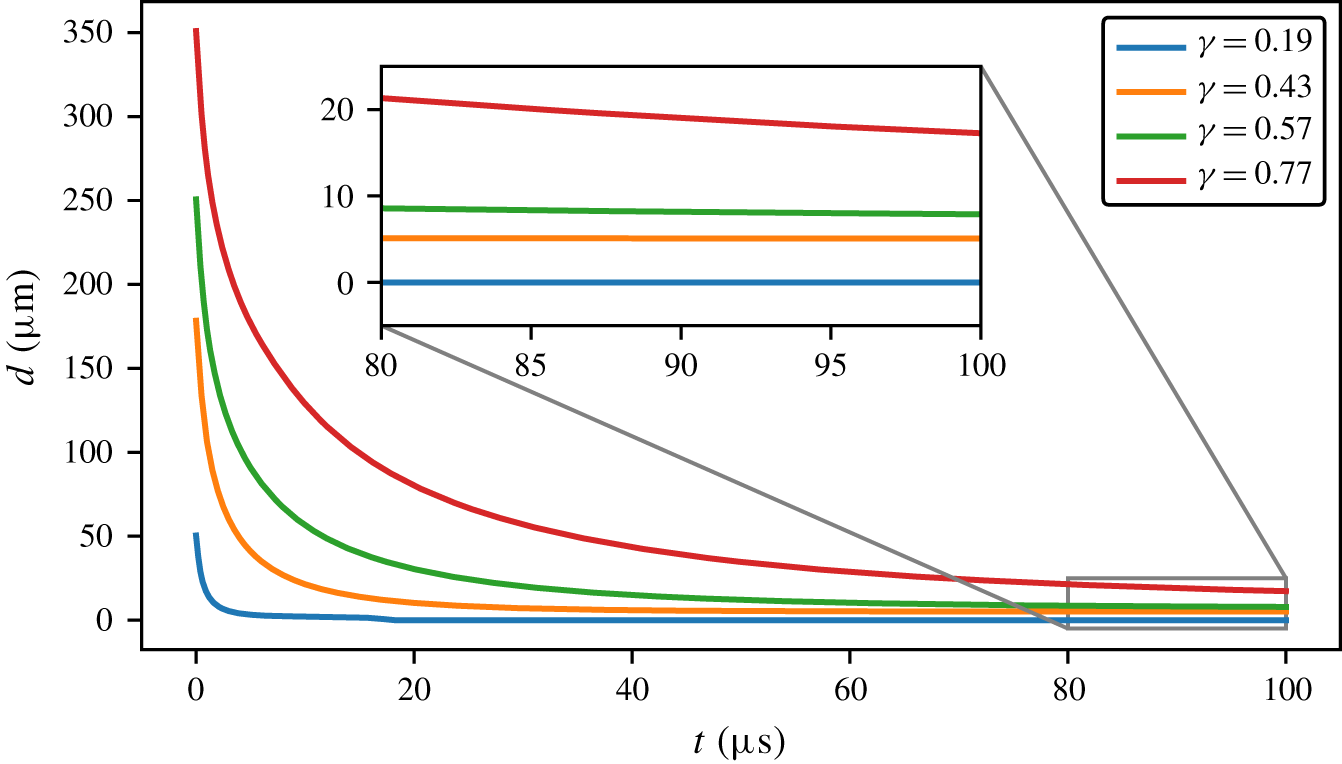
The liquid film between the bubble and the lower wall has a great influence on jet formation, especially for the transferred jet where the film is extremely thin. The experimental set-up can only measure a thickness greater than the pixel size, i.e.  $18~\unicode[STIX]{x03BC}\text{m}$, which is not sufficient to measure the film thickness most of the time. In contrast, simulations reproduce sufficiently well the film dynamics. The simulation results are shown in figure 11, where the film dynamics for bubbles with
 $\unicode[STIX]{x1D6FE}=0.19$, 0.43, 0.57 and 0.77 in a gap of
 $840~\unicode[STIX]{x03BC}\text{m}$ in height are compared. Here the film thickness
 $d$ is defined as the distance between the bubble’s lower interface and the lower wall. Overall
 $d$ decreases rapidly during the early expansion and reaches a constant thickness later. Both the time when the film reaches constant thickness and the thickness decrease with
 $\unicode[STIX]{x1D6FE}$.
Simulation results of liquid film dynamics for various  $\unicode[STIX]{x1D6FE}$. Here
 $H=840~\unicode[STIX]{x03BC}\text{m}$,
 $P_{0}=1000~\text{bar}$,
 $R_{max}\approx 526~\unicode[STIX]{x03BC}\text{m}$.

The current numerical set-up can capture a liquid film with a minimum thickness of approximately  $1.5~\unicode[STIX]{x03BC}\text{m}$, i.e. the cell height. Once the film thickness is smaller than the cell height, a numerical dewetting is considered (see
 $\unicode[STIX]{x1D6FE}=0.19$). Yet the physics of film drainage due to an expanding bubble with small
 $\unicode[STIX]{x1D6FE}$ is still not understood neither experimentally nor by simulations. Thus a reliable model for the dewetting problem is not possible yet.
4 Discussion
4.1 Mechanism of jet formation and jet regimes
From the experimental and particularly the simulation results we find that jet formation is affected by three flow features. Firstly, the shear flow in the gap formed by the expanding bubble and the rigid boundary is deflected away from the boundary by the adverse pressure gradient developed during the late expansion stage (e.g. see time  $t=87~\unicode[STIX]{x03BC}\text{s}$ in figure 3 and time
 $t=85~\unicode[STIX]{x03BC}\text{s}$ in figure 5). This boundary layer instability has been reported previously for thin gaps by Mohammadzadeh et al. (Reference Mohammadzadeh, Li and Ohl2017). The deflected flow merges with the central flow and accelerates the shrinkage of the bubble near the centre of the gap. This is particularly pronounced when the bubble is expanding close to the centre of the gap where both deflected boundary layer flows add. While the bubble shape deforms initially only mildly by the deflected flow, the deformation grows during collapse and develops into an annular flow towards the axis of symmetry. We refer to this flow as ‘splitting flow’ since it splits the bubble. Secondly, when the bubble bottom is very close to the boundary, e.g. figures 2 and 6, the lower edge of the bubble kinks and an annular back flow near the boundary is formed when the bubble shrinks. This kinked annular jet forms a stagnation point on the axis of symmetry and deflects away from the boundary layer, i.e. a jet flow away from the boundary, namely the transferred jet as shown in figure 2. The third feature is the conventional jet flow also seen for bubbles near a single boundary. If the bubble interface is sufficiently far from the upper boundary and thus not affected by the boundary layer, a directed jet is formed.
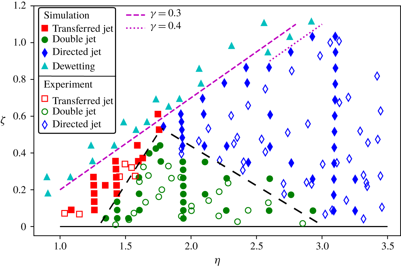
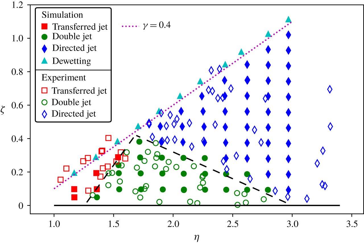
Phase diagram for various induced jets for a gap length of  $L=5~\text{mm}$. Experimental data and computed results are plotted as open and filled symbols, respectively. For both sets of results, square, circle and diamond symbols represent the transferred jet, the double jet and the directed jet, respectively. The dewetting cases from simulation are plotted as filled cyan triangles. The black line is
 $\unicode[STIX]{x1D701}=0$ while the magenta dashed and dotted lines are the stand-off distance from the closer wall
 $\unicode[STIX]{x1D6FE}=0.3$ and
 $\unicode[STIX]{x1D6FE}=0.4$. The black dashed lines are drawn for guiding the transitions. Note that due to symmetry, neither transferred jet nor directed jet occurs at
 $\unicode[STIX]{x1D701}=0$.

Figure 12 summarizes the measured and simulated jets in a phase diagram by describing the geometry with the normalized gap height  $\unicode[STIX]{x1D702}$ and the stand-off distance
 $\unicode[STIX]{x1D701}$. Filled symbols in figure 12 are the computed results while the open symbols are from the experiment. The square, circle and diamond symbols represent the formation of transferred jet, double jet and directed jet, respectively. In the experiment, the equivalent bubble radius varies from
 $R_{max}\approx 520~\unicode[STIX]{x03BC}\text{m}$ to
 $R_{max}\approx 580~\unicode[STIX]{x03BC}\text{m}$, while in the simulation we keep the nucleated radius
 $R_{0}=50~\unicode[STIX]{x03BC}\text{m}$ and pressure
 $P_{0}=1250~\text{bar}$ of the bubble fixed and obtain maximum bubble radii in a slightly narrower range from
 $550$ to
 $580~\unicode[STIX]{x03BC}\text{m}$. An artificial dewetting of the lower wall by the bubble is found in the simulation when the bubble is nucleated very close to the wall. This is the result of insufficient numerical resolution as the physics of the process is not implemented in the simulations. These unreliable points are shown as triangle symbols in the map. The experimental set-up does not allow distinguishing between wetted and dewetted boundaries either. Also, notice from figure 12 that for a wider gap (larger
 $\unicode[STIX]{x1D702}$) the numerical dewetting occurs at larger
 $\unicode[STIX]{x1D6FE}$. Next, we only consider bubbles without dewetting.
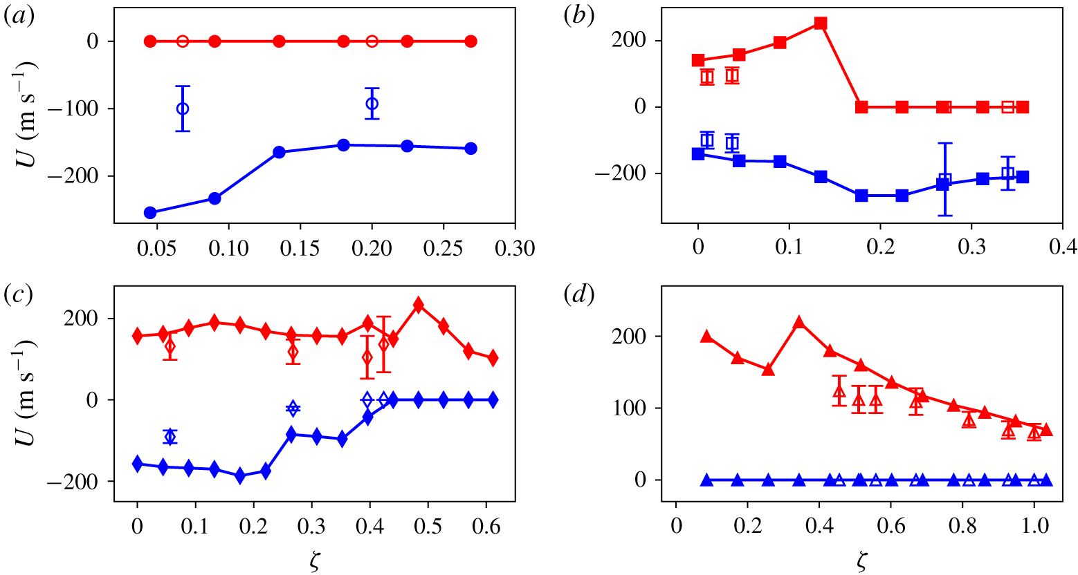
Jet impact velocities as a function of  $\unicode[STIX]{x1D701}$ for selected values of
 $\unicode[STIX]{x1D702}$: (a)
 $\unicode[STIX]{x1D702}=1.26$; (b)
 $\unicode[STIX]{x1D702}=1.43$; (c)
 $\unicode[STIX]{x1D702}=1.93$; (d)
 $\unicode[STIX]{x1D702}=3.10$. The positive direction is downwards to the closest boundary. The blue symbols indicate an upward jet impacting onto the upper and distant wall, thus negative; the red symbols represent the downward jets impacting on the lower wall (positive). Open symbols are from experiments and filled symbols from simulations.

The phase diagram in figure 12 can be divided with two dashed lines shown in black into three regions labelled red (transferred jet), green (double jet) and blue (direct jet). The transferred jet occurs only for  $\unicode[STIX]{x1D702}<1.8$, while the double jet is seen for
 $1.3<\unicode[STIX]{x1D702}<2.8$ and the directed jet only for sufficiently large gaps,
 $\unicode[STIX]{x1D702}>1.8$. We now discuss the transitions between the regimes and show a dependence of the off-centre distance
 $\unicode[STIX]{x1D701}$ on the dimensionless gap height
 $\unicode[STIX]{x1D702}$. Note that due to the symmetry, a bubble nucleated at the centre of the gap (
 $\unicode[STIX]{x1D701}=0$) is not able to produce a transferred jet or a directed jet. The experiments and simulations show that the transition between the transferred jet and the double jet regimes increases between
 $\unicode[STIX]{x1D702}\approx 1.3$ and
 $\unicode[STIX]{x1D702}\approx 1.8$ with a slope of about
 $1$. The reason is that, as the gap height increases, the bubble needs to be nucleated closer to the wall so that its lower interface remains within the viscous boundary layer. Only then does it produce a sharp edge and a strong edge flow during the collapse, which causes the transferred jet. The second parameter boundary between the double jet and the directed jet regime occurs between
 $\unicode[STIX]{x1D702}\approx 1.8$ and
 $\unicode[STIX]{x1D702}\approx 2.8$. Here the slope is approximately
 $-0.4$. The negative slope can be explained in that as
 $\unicode[STIX]{x1D702}$ increases, the focusing flow on the bubble top surface strengthens due to a weaker influence from the top rigid boundary. Therefore for the double jet to occur, the bubble nucleation site needs to be moved closer to the centre of the gap to weaken the vertical focusing flow and enhance the splitting flow. For
 $\unicode[STIX]{x1D702}>3.0$, the focusing flow on the distant bubble wall is dominating, which results in the well-known jetting towards the closest boundary.
4.2 Effect of geometry on jet impact velocity
Here we compare the experimentally and numerically obtained velocities of the jets impacting on the boundaries as a function of the bubble position for four selected gap heights. Unfortunately in the experiments we have only two to three frames available to measure the velocity. Therefore, we limit this comparison to that of an averaged measure of the jet velocity before impact. For this we need to determine the distance and time from jet formation until impact and define the start of the jet formation, which is different for the distinct jetting scenarios. Here, we choose for the transferred jet the time of detachment of the bubble interface from the boundary, for the double jet the time of pinch-off and for the directed jet the time the bubble wall on the axis of symmetry reaches a constant velocity (slow jet) or strong acceleration occurs (fast jet, e.g. figure 7 at  $t=152.5~\unicode[STIX]{x03BC}\text{s}$). In the simulation, the time of jet impact for all cases is identified as the instant the liquid flow with a diameter larger than 2 mesh cells
 $(2\times 1.5~\unicode[STIX]{x03BC}\text{m})$ reaches the wall. However, in the experiments, the impact time may be overestimated due to the inherent limitations in determining the exact time of jet creation and impact on the wall; thus the experimental jet velocities reported here represent a lower bound.
While the average velocity underestimates the tip velocity, it nevertheless provides a good indication as to when the fastest jets are to be expected. The uncertainty in the experimental determination is calculated from  $\unicode[STIX]{x0394}V/V=((\unicode[STIX]{x0394}S/S)^{2}+(\unicode[STIX]{x0394}T/T)^{2})^{1/2}$, where
 $V$ is the calculated jet velocity,
 $S$ and
 $T$ are the travel distance and time interval from formation to impact and
 $\unicode[STIX]{x0394}S=18~\unicode[STIX]{x03BC}\text{m}$ and
 $\unicode[STIX]{x0394}T=1~\unicode[STIX]{x03BC}\text{s}$ are the spatial and temporal resolutions, respectively.
Impact jet velocities for the four non-dimensional gap heights  $\unicode[STIX]{x1D702}=1.26,1.43,1.93$ and
 $3.10$ are plotted in figure 13. In the simulations we only vary the gap height
 $H$ and keep the initial conditions (
 $R_{0}=50~\unicode[STIX]{x03BC}\text{m}$ and pressure
 $P_{0}=1250~\text{bar}$) the same. For each value of
 $\unicode[STIX]{x1D702}$ the resulting bubble volume versus time curves up to the first minimum volume are nearly indistinguishable. The averaged impact velocity onto the closer boundary is defined positive and plotted in red while the impact velocity onto the distant wall is negative and coloured blue. The experimental data are shown with open symbols while the computed results are plotted with filled symbols.
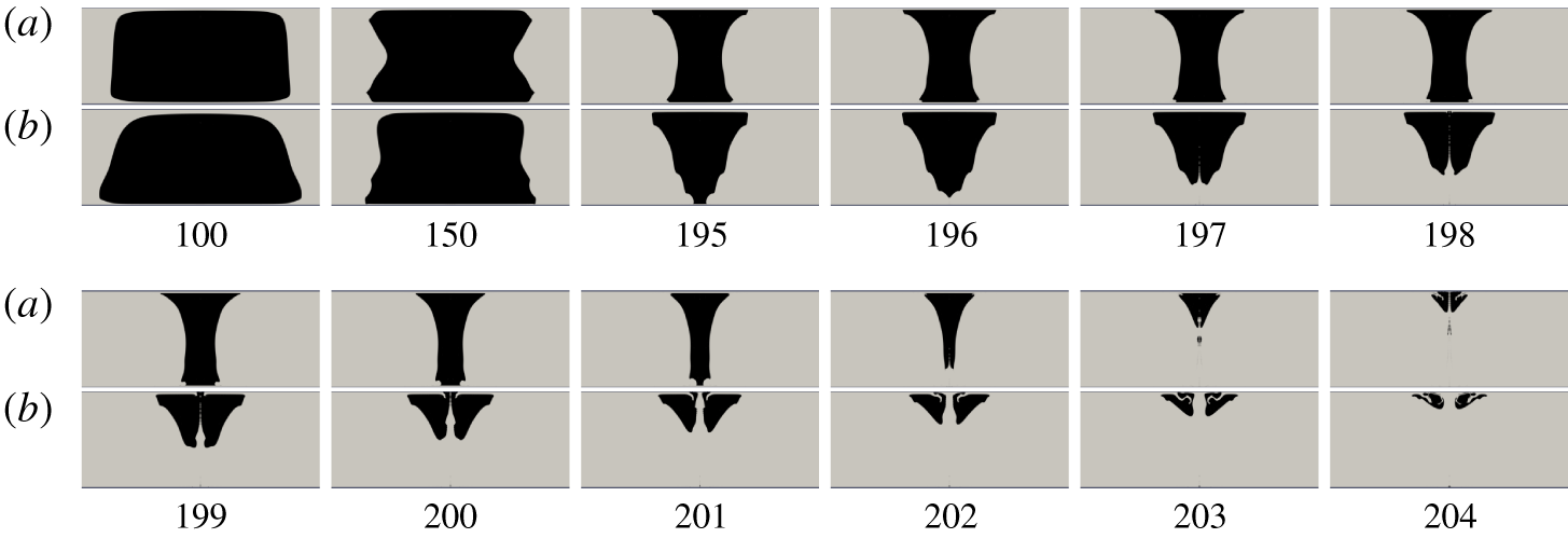
Comparison of jet dynamics for  $\unicode[STIX]{x1D702}=1.26$ when the bubble is created close to the centre at
 $\unicode[STIX]{x1D701}=0.03$ (a) and further away at
 $\unicode[STIX]{x1D701}=0.14$ (b). The gap height is
 $H=700~\unicode[STIX]{x03BC}\text{m}$ and times are stated in microseconds.

For sufficiently thin gaps, here  $\unicode[STIX]{x1D702}=1.26$, all non-zero values of
 $\unicode[STIX]{x1D701}$ lead to a transferred jet as visible in figure 12. Yet, in the simulations the transferred jet velocity varies with the position of bubble creation, i.e. the value of
 $\unicode[STIX]{x1D701}$. Figure 13(a) shows that the velocity for small
 $\unicode[STIX]{x1D701}$ (near the centre of the gap) is approximately twice the velocity as compared to larger
 $\unicode[STIX]{x1D701}$. To obtain some insight, we compare the bubble dynamics for
 $\unicode[STIX]{x1D701}=0.03$ (fast jet) and
 $\unicode[STIX]{x1D701}=0.14$ (slow jet) in figure 14. For
 $\unicode[STIX]{x1D701}=0.03$, the bubble expands first to approximately a rectangle at
 $t=100~\unicode[STIX]{x03BC}\text{s}$ and shrinks to a vertical cylinder shape before it detaches from the lower wall at
 $t=201~\unicode[STIX]{x03BC}\text{s}$. In contrast, the bubble at
 $\unicode[STIX]{x1D701}=0.14$ loses the fore-and-aft symmetry early at maximum expansion and obtains the shape of an inverted cone at
 $t=195~\unicode[STIX]{x03BC}\text{s}$. Bubbles losing their symmetry early during the collapse (
 $\unicode[STIX]{x1D701}=0.14$) develop a slower jet than bubbles with a more symmetric collapse
 $(\unicode[STIX]{x1D701}=0.03)$. We find averaged jet velocities of approximately
 $250~\text{m}~\text{s}^{-1}$ for
 $\unicode[STIX]{x1D701}=0.03$ and
 $140~\text{m}~\text{s}^{-1}$ for
 $\unicode[STIX]{x1D701}=0.14$. The reason for the faster jets is likely the higher stagnation pressure due to the higher velocities and the smaller amount of liquid comprising the jet.
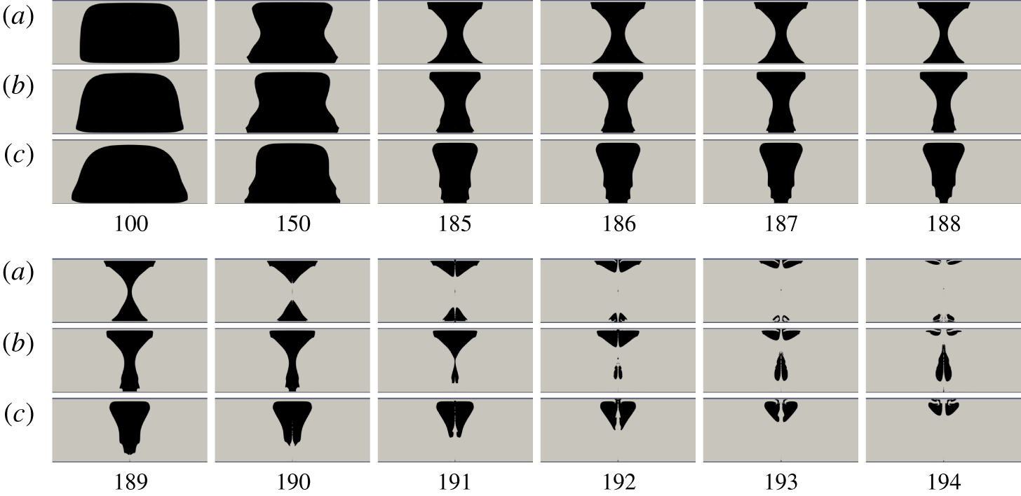
Comparison of jet dynamics for  $\unicode[STIX]{x1D702}=1.43$ when the bubble is created close to the centre at
 $\unicode[STIX]{x1D701}=0.09$ (a),
 $\unicode[STIX]{x1D701}=0.18$ (b) and
 $\unicode[STIX]{x1D701}=0.31$ (c). The gap height is
 $H=800~\unicode[STIX]{x03BC}\text{m}$ and times are stated in microseconds.

For a larger gap height at  $\unicode[STIX]{x1D702}=1.43$, the bubble crosses the boundary from the double jet regime for small
 $\unicode[STIX]{x1D701}$ to the transferred jet regime. This transition is shown in figure 15 with the bubble dynamics for
 $\unicode[STIX]{x1D701}=0.09$,
 $0.18$ and
 $0.31$. For
 $\unicode[STIX]{x1D701}=0.09$, the bubble splits approximately at the gap’s centre between
 $t=189~\unicode[STIX]{x03BC}\text{s}$ and
 $t=190~\unicode[STIX]{x03BC}\text{s}$ resulting in two jets impacting the lower and upper boundary with a velocity of about
 $190$ and
 $160~\text{m}~\text{s}^{-1}$, respectively. At an increased
 $\unicode[STIX]{x1D701}$ of 0.18, the bubble splits
 $1~\unicode[STIX]{x03BC}\text{s}$ later at
 $t=191~\unicode[STIX]{x03BC}\text{s}$. But then the two daughter bubbles jet in the same directions to the upper boundary. The velocity of this transferred jet from the upper daughter bubble is
 $260~\text{m}~\text{s}^{-1}$. On increasing
 $\unicode[STIX]{x1D701}$ to 0.31, the bubble does not split and a single transferred jet is found now with a lower velocity of about
 $200~\text{m}~\text{s}^{-1}$. A summary of velocity versus
 $\unicode[STIX]{x1D701}$ is plotted in figure 13(b). The double jet is formed at
 $0<\unicode[STIX]{x1D701}<0.15$; in this regime the jet velocities (absolute values) on both walls increase along with
 $\unicode[STIX]{x1D701}$. The transferred jet occurs when
 $\unicode[STIX]{x1D701}>1.8$ and its evolution is similar to that in figure 13(a).
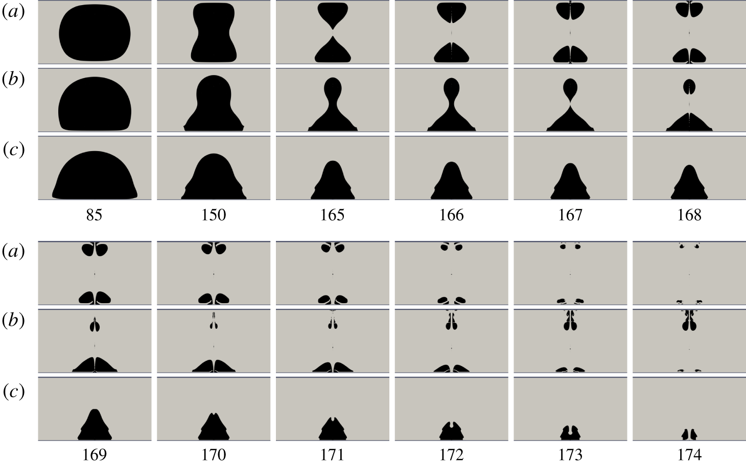
Comparison of jet dynamics for  $\unicode[STIX]{x1D702}=1.93$ when the bubble is nucleated at
 $\unicode[STIX]{x1D701}=0.04$ (a),
 $\unicode[STIX]{x1D701}=0.31$ (b) and
 $\unicode[STIX]{x1D701}=0.57$ (c). The gap height
 $H=1100~\unicode[STIX]{x03BC}\text{m}$ and times are stated in microseconds.

For a larger gap,  $\unicode[STIX]{x1D702}=1.93$, the bubble moves from the double jet regime to the directed jet regime as
 $\unicode[STIX]{x1D701}$ increases. We compare the jet dynamics at
 $\unicode[STIX]{x1D701}=0.04$, 0.31 and 0.57 in figure 16 and plot the velocity in figure 13(c). For
 $\unicode[STIX]{x1D701}=0.04$, the bubble attaches to both walls and splits into two daughter bubbles with approximately equal size. This is also seen in figure 13(c) where the impacting jet velocities on both walls are comparable at
 $0<\unicode[STIX]{x1D701}<0.22$ with little variation. For
 $\unicode[STIX]{x1D701}=0.31$, the bubble only attaches to the lower wall and releases a smaller daughter bubble moving upwards when splitting. This bubble impacts the upper wall at a later time with a lower velocity compared to the attached daughter bubble. Similar dynamics happens at
 $0.27<\unicode[STIX]{x1D701}<0.45$, as shown in figure 13(c). For
 $\unicode[STIX]{x1D701}\geqslant 0.45$, the bubble collapses onto the lower wall and induces a directed jet, whose velocity decreases with increasing
 $\unicode[STIX]{x1D701}$.
Comparison of jet dynamics for  $\unicode[STIX]{x1D702}=3.10$ when the bubble is nucleated at
 $\unicode[STIX]{x1D701}=0.34$ (a) and
 $\unicode[STIX]{x1D701}=0.86$ (b). The gap height
 $H=1800~\unicode[STIX]{x03BC}\text{m}$ and times are stated in microseconds.

Increasing the gap height  $\unicode[STIX]{x1D702}$ to 3.10 makes the bubble collapse only onto the lower wall with a directed jet. Two selected induced jet dynamics at
 $\unicode[STIX]{x1D701}=0.34$ and
 $\unicode[STIX]{x1D701}=0.86$ are compared in figure 17. At
 $\unicode[STIX]{x1D701}=0.34$, the bubble expands to a sphere at
 $t=75~\unicode[STIX]{x03BC}\text{s}$ and shrinks acquiring a dripping water droplet shape before jet formation at
 $t=142~\unicode[STIX]{x03BC}\text{s}$. The sharp top interface pierces through the bubble and develops a directed jet impacting the wall with a velocity up to
 $220~\text{m}~\text{s}^{-1}$ at
 $t=146~\unicode[STIX]{x03BC}\text{s}$. At a higher
 $\unicode[STIX]{x1D701}$ of 0.86, the bubble expands to a hemisphere at
 $t=75~\unicode[STIX]{x03BC}\text{s}$ and collapses to a cone at
 $t=135~\unicode[STIX]{x03BC}\text{s}$, developing a jet with a velocity of about
 $90~\text{m}~\text{s}^{-1}$ impacting at
 $t=145~\unicode[STIX]{x03BC}\text{s}$. In figure 13(d), the impact velocity for
 $0<\unicode[STIX]{x1D701}<0.3$ is from the re-entrant vapour jet where the bubble is far away from the boundary. For
 $\unicode[STIX]{x1D701}>0.34$, the jet velocity decreases with
 $\unicode[STIX]{x1D701}$ as the bubble is closer to the wall.
(a) Comparison of the equivalent spherical bubble radius for various gap radii from simulations. The gap height  $H=0.7~\text{mm}$ and the distance to the closer wall
 $h=250~\unicode[STIX]{x03BC}\text{m}$ are kept constant. The bubble dynamics converges at
 $L=180~\text{mm}$. (b) The expansion time and collapse time versus gap radius. Note that the time is normalized by the Rayleigh collapse time.

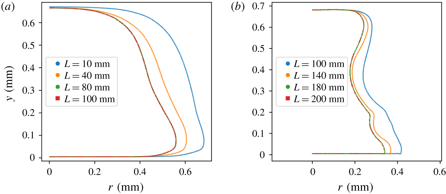
The bubble interface. (a) The late expansion at  $t=100~\unicode[STIX]{x03BC}\text{s}$; the bubble shape converges at
 $L=80~\text{mm}$. (b) The late collapse at
 $t=200~\unicode[STIX]{x03BC}\text{s}$; the bubble shape converges at
 $L=180~\text{mm}$.

4.3 Influence of the gap length  $L$

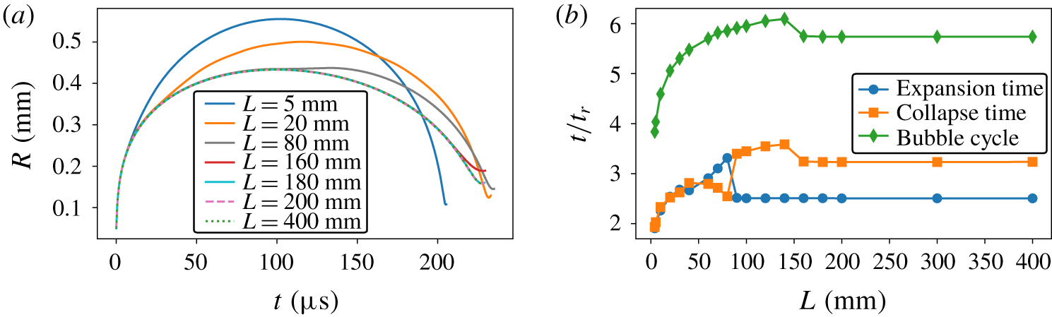
In this section we investigate the influence of the gap length  $L$ on the bubble dynamics. Figure 18(a) compares the temporal evolution of the equivalent bubble radius and figure 18(b) shows the expansion and collapse time of the bubble from
 $L=5~\text{mm}$ to
 $L=400~\text{mm}$ for bubbles under the same initial condition and gap height. The constant parameters are
 $H=0.7~\text{mm}$,
 $h=250~\unicode[STIX]{x03BC}\text{m}$,
 $R_{0}=50~\unicode[STIX]{x03BC}\text{m}$ and
 $P_{0}=1250~\text{bar}$. The expansion and collapse times are defined as the interval from the nucleation to the maximum size and from the maximum size to the minimum size, respectively. The time shown in figure 18(b) is normalized by the Rayleigh collapse time
 $t_{r}=0.915R_{max}(\unicode[STIX]{x1D70C}/\unicode[STIX]{x0394}P)^{1/2}$ (Brennen Reference Brennen2014). In figure 18(a) we find that
 $R_{max}$ decreases with gap length. This may be explained by viscous losses from the flow in the gap that are reducing the potential energy of the bubble, i.e. during maximum volume. Also, we observe a fluctuation of the expansion time versus collapse between
 $L=60~\text{mm}$ and
 $L=90~\text{mm}$. This is the result of the bubble’s internal pressure expanding some parts of the bubble into the liquid that is backed by a lower pressure. As a result, the bubble undergoes a longer expansion than collapse (see
 $60~\text{mm}<L<90~\text{mm}$ in figure 18b). This fluctuation vanishes when this kind of local bubble expansion is suppressed by the then stronger viscous boundary layer flow. This local expansion disappears for
 $L>90~\text{mm}$, where the expansion time shrinks below the collapse time (see figure 18b). For larger gap lengths of
 $L>180~\text{mm}$, the bubble dynamics becomes independent of
 $L$. This convergence of the dynamics is also documented in figure 19, where the bubble interface for various
 $L$ is shown for the same times, namely for late expansion
 $t=100~\unicode[STIX]{x03BC}\text{s}$ and during collapse
 $t=200~\unicode[STIX]{x03BC}\text{s}$ in figures 19(a) and 19(b), respectively. Overall, the oscillation time is considerably longer than the Rayleigh oscillation time and increases with
 $L$ before it reduces and settles to a constant value. For large
 $L$ the collapse time is always longer than the expansion time. This is likely caused by the opposing flow in the boundary layer hindering a simple inflow. Viscosity breaks here the symmetry between the flows driving bubble expansion and bubble collapse.
Phase diagram for the induced jet for gap radius of  $L=13~\text{mm}$. Experimental data and computed results are plotted as open and filled symbols, respectively. For each set of results, the square, circle and diamond symbols represent the transferred jet, the double jet and the directed jet, respectively. The dewetting cases from simulation are plotted as filled cyan triangles. The black line is
 $\unicode[STIX]{x1D701}=0$ while the magenta dotted line is the stand-off distance from the closer wall
 $\unicode[STIX]{x1D6FE}=0.4$. The black dashed lines are drawn for guiding the transitions. Note that due to symmetry, neither transferred jet nor directed jet occurs at
 $\unicode[STIX]{x1D701}=0$.

Next, we discuss the importance of the gap length on the jetting behaviour. The phase diagram for jetting in figure 20 uses a wider gap of  $L=13~\text{mm}$ as compared to the experiments and simulation presented previously in figure 12 with
 $L=5~\text{mm}$. Overall, the new phase diagram shares many features of figure 12 with three distinct regimes. Yet, there are some differences. Firstly, the dewetting transition increases to
 $\unicode[STIX]{x1D6FE}=0.4$ for the whole parameter range in the plot. Secondly, the transferred jet regime becomes narrower. A bubble loses more energy in a gap with larger
 $L$, and thus the motion of the edge annular flow is slowed down during the collapse, which makes it more difficult for the bubble to produce the transferred jet in the small-
 $\unicode[STIX]{x1D702}$ regime. In the large-
 $\unicode[STIX]{x1D702}$ domain, it is easier for the bubble to collapse on the closer wall than split into two bubbles as a gap with longer radius reduces the confined effect of the upper wall, which makes it easier for the fluid to focus on the bubble top interface and flows downwards.
4.4 Influence of liquid viscosity
We present exemplarily the effect of an increased liquid viscosity. Liquids with a larger viscosity than the previously studied water case develop thicker boundary layers (Schlichting & Gersten Reference Schlichting and Gersten2016). This affects the bubble growth close to the walls. Figure 21 compares the simulated bubble dynamics for the same initial location, gap height and initial conditions as shown in figure 2, however now with a liquid viscosity of  $20~\text{cSt}$. The water case with a viscosity of
 $1~\text{cSt}$ is overlaid in figure 21 with the help of an orange line. Interestingly the maximum bubble radius,
 $R_{max}=526~\unicode[STIX]{x03BC}\text{m}$, is hardly affected and thus
 $\unicode[STIX]{x1D702}=1.60$ and
 $\unicode[STIX]{x1D701}=0.37$ remain unchanged as compared to the the water case. Yet, the overall bubble dynamics is greatly affected. This becomes evident in that in the water case, figure 2, the bubble develops a transferred jet while here it splits into two jets. The liquid film between the bubble and the lower wall increases from
 $5~\unicode[STIX]{x03BC}\text{m}$ for water to about
 $15~\unicode[STIX]{x03BC}\text{m}$. Additionally the bubble edges are lifted away from the lower wall. At maximum expansion, the lifting of the lower rim is about
 $130~\unicode[STIX]{x03BC}\text{m}$, considerably higher than that in water of approximately
 $40~\unicode[STIX]{x03BC}\text{m}$. This larger distance resembles the scaling of the boundary layer thickness
 $\unicode[STIX]{x1D6FF}\sim \sqrt{\unicode[STIX]{x1D707}/\unicode[STIX]{x1D70C}}$ (Gonzalez-Avila, Song & Ohl Reference Gonzalez-Avila, Song and Ohl2015). Due to higher resistance to shear in a viscous liquid, the surface of the bubble is smoother with less pronounced kinks that appear only after
 $t>200~\unicode[STIX]{x03BC}\text{s}$. During the collapse, the region near the lifted-up rim has the highest pressure gradient accelerating the flow inwards first (see
 $t=110$, 150 and
 $170~\unicode[STIX]{x03BC}\text{s}$). Yet, as this inflow is further away from the wall it induces a ‘splitting flow’ with the formation of double jets.
Computed bubble dynamics in a viscous liquid with  $\unicode[STIX]{x1D707}=20~\text{cSt}$. The numerical conditions are the same as the case in figure 2, except for the liquid viscosity. The computed results are with
 $R_{max}=526~\unicode[STIX]{x03BC}\text{m}$,
 $\unicode[STIX]{x1D702}=1.60$ and
 $\unicode[STIX]{x1D701}=0.37$. Times are stated in microseconds. The orange contours indicate the bubble dynamics of water from figure 2.

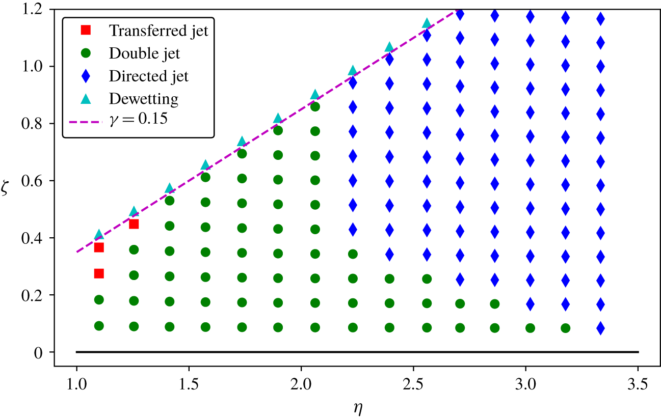
Phase diagram for jets in a liquid with a viscosity of 20 cSt. Gap length  $L=5~\text{mm}$. The computed results are plotted as filled symbols. Square, circle and diamond symbols represent the transferred jet, the double jet and the directed jet, respectively. The dewetting cases from simulation are plotted as filled cyan triangles. The black line is
 $\unicode[STIX]{x1D701}=0$ while the magenta dashed line is the stand-off distance from the closer wall
 $\unicode[STIX]{x1D6FE}=0.15$. Note that due to symmetry, neither transferred jet nor directed jet occurs at
 $\unicode[STIX]{x1D701}=0$.

To investigate the viscous effect on the jetting regimes, here we keep constant the liquid viscosity at  $\unicode[STIX]{x1D707}=20~\text{cSt}$ and report the simulation results in figure 22. The result is compared to figure 12 to reveal the viscous effect. First of all, the dewetting transition is found decreasing to
 $\unicode[STIX]{x1D6FE}=0.15$, since the liquid film between the bubble and walls becomes thicker as the viscosity of liquid increases. The phase diagram also contains three distinct regimes. Among them, the transferred jet is only seen for very small
 $\unicode[STIX]{x1D702}$ and relatively large
 $\unicode[STIX]{x1D701}$, which means it only happens in very narrow gaps and when the bubble is nucleated very close to the lower wall. Comparing the regimes in figures 12 and 22, we find that the transferred jet is suppressed while the double jet is facilitated in a more viscous liquid. Moreover, for
 $1.4\leqslant \unicode[STIX]{x1D702}\leqslant 2.1$, only the double jet is seen. The reason is that, as viscosity enhances the confined effect of the walls, both the edge annular flow near the lower wall and the vertical focusing flow on the bubble’s top surface become weaker. Once the gap is large enough (
 $\unicode[STIX]{x1D702}\geqslant 2.2$) the vertical focusing flow strengthens, and therefore a directed jet can be formed. In general, it requires a larger gap to induce a directed jet in a more viscous liquid.
5 Conclusions
With the confinement of two parallel rigid walls, a bubble experiences distinct scenarios of jetting. Here, the importance is laid on the effect of the gap height and location of the bubble nucleation within that gap. The results from our experiments and simulations are collected and summarized over a large range of parameters. The axisymmetric simulations that account for the liquid viscosity, compressibility and surface tension are in good agreement with the experiments. In particular they not only predict well the overall shape and timing but also the complex deformation of the near-wall bubble interface.
The flow fields and pressure distribution obtained from the axisymmetric simulations reveal the mechanism of jetting: it is a competition between the splitting flow, the annular edge flow and the vertically inward flow. Viscosity is crucial for developing the fast annular edge flow very close to the wall and was absent in earlier simulations (Gonzalez-Avila et al. Reference Gonzalez-Avila, Klaseboer, Khoo and Ohl2011b; Hsiao et al. Reference Hsiao, Choi, Singh, Chahine, Hay, Ilinskii, Zabolotskaya, Hamilton, Sankin and Yuan2013) using the inviscid boundary element method.
The two dimensionless variables  $\unicode[STIX]{x1D701}$ and
 $\unicode[STIX]{x1D702}$ allow the construction of a phase diagram of the jetting scenarios based on experiments and simulations. In a sufficiently narrow gap, the bubble can jet towards the distant wall,
 $\unicode[STIX]{x1D702}<1.3$. This was first reported by Gonzalez-Avila et al. (Reference Gonzalez-Avila, Klaseboer, Khoo and Ohl2011b) where the bubble was nucleated close to one wall. There, for small
 $\unicode[STIX]{x1D702}$, the bubble translated to the distant wall, while for even smaller
 $\unicode[STIX]{x1D702}$ the bubble became disc-shaped and collapsed between the two walls. Recently Quah et al. (Reference Quah, Karri, Ohl, Klaseboer and Khoo2018) reproduced the experiment with larger spark-generated bubbles in the small-
 $\unicode[STIX]{x1D702}$ regime and observed the dynamics from the side and from below (through a transparent boundary). They pointed out that once the gap height decreases below a certain value, the jet will impact on the closer wall. That contradicts the regime where Gonzalez-Avila et al. (Reference Gonzalez-Avila, Klaseboer, Khoo and Ohl2011b) observed the disc-shaped bubble collapsing between the two walls. Based on our current results, the discrepancy between these two studies may come from the pinning effect of the walls in the dewetting regime. As shown in figure 12, the range of
 $\unicode[STIX]{x1D701}$ allowing a transferred jet becomes smaller as
 $\unicode[STIX]{x1D702}$ decreases, meaning it is easier for the bubble to touch the near wall in a gap with smaller
 $\unicode[STIX]{x1D702}$. Once the thin liquid film has drained, the bubble dynamics can be greatly affected by the surface properties of the substrate. Our current model does not account for the three-phase contact line dynamics. Therefore we cannot provide predictions for the jet dynamics in the dewetted regime. Hence a time dependency on the film drainage is expected and a scaling by the bubble radius alone may not be sufficient, i.e.
 $\unicode[STIX]{x1D702}$ and
 $\unicode[STIX]{x1D701}$ do not span the parameter space. Thus, further studies with an appropriate model for the contact line dynamics could supplement the phase diagrams shown here. The thickness of the substrate may be studied using a recently invented technique (Reuter & Kaiser Reference Reuter and Kaiser2019).
For intermediate  $\unicode[STIX]{x1D702}$, a bubble may split into two daughter bubbles impacting on both walls. If the bubble is nucleated near the gap centre, e.g.
 $\unicode[STIX]{x1D701}$ is small, the bubble splits almost symmetrically around the centre of the gap. Then two daughter bubbles are created with similar size and accompanying fast jet impacting of up to
 $200~\text{m}~\text{s}^{-1}$. When the bubble is off-centre, it undergoes an asymmetric splitting, releasing a small bubble with slower speed jetting towards the upper wall and a larger part impacting onto the lower wall. Theoretically, the impact speed onto the upper wall can be adjusted with the off-centre position, which would allow the design of a geometry for a specific impact velocity.
The directed jet develops from a bubble that takes the shape of a cone during the early collapse (see figure 6). The velocity at impact decreases with  $\unicode[STIX]{x1D701}$ from more than
 $200$ to
 $100~\text{m}~\text{s}^{-1}$. Recently Lechner et al. (Reference Lechner, Lauterborn, Koch and Mettin2019) reported simulation results of a bubble collapsing near a single boundary. For very small stand-off distances, a novel collapse scenario was reported that demonstrated an order-of-magnitude increase in the jet velocity as compared to slightly larger distances. Their case with
 $\unicode[STIX]{x1D6FE}=0.048$ and a jet velocity of
 $1000~\text{m}~\text{s}^{-1}$ has some similarities with the case presented in figure 6. We see in both cases the rapid deceleration of the flow forming a region with a high positive pressure and the emission of a pressure transient that accelerates the liquid at a curved interface to a high velocity. While there are some striking similarities, the present case (figures 7–9) reaches a lower tip velocity of
 $580~\text{m}~\text{s}^{-1}$. A plausible reason may be that the jet from Lechner et al. (Reference Lechner, Lauterborn, Koch and Mettin2019) is formed at an even later stage of the collapse, where the pressure at the top of the tip is higher due to the faster velocities. Also, the particular shape of the conical tip may affect the resulting tip velocity.
The width of the gap also affects the bubble dynamics. Previously Gonzalez-Avila et al. (Reference Gonzalez-Avila, Klaseboer, Khoo and Ohl2011b) using the boundary element method commented that the collapse time increases with the length of the axisymmetric gap. The present work confirms this observation but also demonstrates that the bubble dynamics with increasing length of the gap eventually converges. With increasing length of the gap, the bubble collapse from maximum volume takes considerably longer than the expansion to maximum volume. We explain this with energy dissipation in the viscous boundary layer. Also, in a wider gap the  $\unicode[STIX]{x1D702},\unicode[STIX]{x1D701}$ region where a transferred jet is observed is smaller.
In summary, the present work covered experimental and simulated bubble dynamics within a narrow gap using the location and bubble size as parameters. The important results are the phase diagrams in figures 12, 20 and 22. While the dynamics of a cavitation bubble near a single rigid boundary has been studied carefully for many years, the present study provides an overview for the next more complex geometry of two parallel boundaries. Here, we want to emphasize the importance of viscous boundary layers for the formation of high-speed jets, similar to the single-wall case (Lechner et al. Reference Lechner, Lauterborn, Koch and Mettin2019). Besides, the jet dynamics (direction and strength) is dependent on the choice of gap thickness and location of bubble inception. Thus, for applications, these two parameters may be chosen to obtain a desired flow pattern.
Acknowledgements
We acknowledge the anonymous referees for their very helpful suggestions to improve the manuscript.
Declaration of interests
The authors report no conflict of interest.