


Throughout most of history, humans typically died before their 40th birthday. Today, life expectancy at birth has surpassed 80 in many advanced economies. A large literature has studied the drivers behind the historical mortality decline (e.g., for overviews, see Cutler, Deaton, and Lleras-Muney (Reference Cutler, Deaton and Lleras-Muney2006) and Costa (Reference Costa2015)). The most prominent explanations include more or higher-quality nutrition due to rising incomes (McKeown Reference McKeown1976), public health interventions (Szreter 1988), and medical progress. The role of social security—and old-age assistance in particular—has received less attention,Footnote 1 even though the emergence of the European welfare state in the late nineteenth and early twentieth centuries coincided with an accelerated reduction in mortality rates.
In this paper, we use the Old-Age Pension Act of 1908, which introduced means-tested public pensions for everybody in the United Kingdom aged 70 or older,Footnote 2 as a quasi-natural experiment to study the impact of old-age assistance on mortality. Using aggregate national mortality data for England and Wales from 1901 to 1913, we show that elderly mortality (age 75+), relative to middle-aged mortality (age 45–64), declined after the pension was introduced. Event-time estimates suggest that the mortality decline started after the first pensions were paid and became larger over time. Using regional-level data, we also show that the decline in elderly mortality was bigger in counties with a higher share of pensioners. Depending on the specification, we estimate that elderly mortality fell by 2.7 to 12.5 percent after the pension was introduced. Taking these estimates at face value, the introduction of old-age assistance could explain a substantial share of the overall elderly mortality decline happening in the United Kingdom between the beginning of the twentieth century and WWII. Combining these findings with the welfare analysis conducted in Giesecke and Jäger (Reference Giesecke and Jäger2021) leaves little doubt that the introduction of public pensions in the United Kingdom increased societal welfare.Footnote 3
We argue that the pension improved health outcomes by reducing residential crowding, thus impeding the spread of infectious diseases, and inducing retirement, especially from occupations associated with high mortality rates. First, we document, based on national-level cause of death data, that the mortality decline was driven by lower elderly mortality from infections and non-infectious diseases (and not by fewer violence-, accident-, or suicide-related deaths). Secondly, exploiting full-count individual-level census data, we show that the average number of residents per household, as a proxy for residential crowding, substantially declined for people aged 70+, relative to people aged 69, after the pension was introduced. The decline is mostly driven by fewer elderly people living in poorhouses (also known as workhouses), which were typically very crowded institutions. Third, following the findings of Giesecke and Jäger (Reference Giesecke and Jäger2021) that the pension reduced elderly labor supply, we document that the labor supply reduction was especially large for people working in occupations associated with very high mortality rates. Regional and gender heterogeneity further support our proposed mechanisms. We show that both mortality and residential crowding declined more in urban compared to rural areas, where Poor Law Relief in poorhouses was more common. We also find that mortality declined at roughly similar rates for men and women, although women had substantially higher rates of pension recipiency. We argue that men’s lower pension recipiency was offset by a stronger behavioral response in terms of household crowding and labor supply. These findings align with historical evidence from the pre-pension period, which suggests that poor elderly men more often relied on Poor Law relief in crowded workhouses and on labor income than did women (Boyer Reference Boyer2019).Footnote 4
The remainder of this paper is structured as follows. In the next section, we compare our study with the existing literature, discussing how our work builds upon and contributes to previous studies. The third section outlines the historical and institutional details of the reform. The fourth section presents the data, empirical strategy, and results of our main analysis, focusing on the impact of the pension reform on national-level mortality. The fifth section provides complementary regional-level evidence, while the sixth section examines mechanisms at the individual level. The seventh section explores heterogeneity by rural-urban status and gender, the eighth section discusses the findings, and the ninth section concludes.
CONTRIBUTION TO THE LITERATURE
So far, econometric studies that draw on the Old-Age Pension Act (OAPA) to study the impact of pensions on health are missing. This absence is surprising, given the unique advantages provided by the historical setting. Comparable evidence on the mortality effects of public pension schemes comes either from contemporary countries with income levels similar to those in Britain in the early twentieth century or from other developed countries during the same historical period. Regarding the former, the OAPA provides the unique opportunity to estimate the mortality effect of transitioning from a situation without any pension program to an old-age assistance scheme that covered a substantial portion of the elderly population. Thereby, we contribute to existing research, which has tended to focus on more limited reforms, either regionally (Huang and Zhang Reference Huang and Zhang2021; Cheng et al. Reference Cheng, Liu, Zhang and Zhao2018; Aguila, Kapteyn, and Smith Reference Aguila, Kapteyn and Smith2015; Galiani, Gertler, and Bando Reference Galiani, Gertler and Bando2016), targeted at specific ethnic groups (Case Reference Case and David2004) or involving only changes to existing pension systems (Jensen and Richter Reference Jensen and Richter2004; Miglino et al. Reference Miglino, Nicolás Navarrete, Gonzalo Navarrete and Pablo Navarrete2023). Comparable evidence from historic pension reforms in now-developed countries primarily stems from studies on the United States (Balan-Cohen Reference Balan-Cohen2008; Stoian and Fishback Reference Stoian and Fishback2010; Galofré-Vilà, McKee, and Stuckler Reference Galofré-Vilà, McKee and Stuckler2022) and Canada (Emery and Matheson 2012). In contrast to these programs that were introduced in the aftermath of the Great Depression, old-age assistance in the United Kingdom was established in a period of stable economic conditions, which ensures that the effects are less confounded by macroeconomic shocks (at least until 1914) or the expansion of other social spending.Footnote 5
Moreover, the OAPA enables us to study a very early public transfer program. This setting has the advantage that mortality was still relatively high, old-age poverty widespread, and other public social assistance largely absent, making it more likely for mortality to respond to means-tested pensions. So far, the only evidence on the role of pensions on health before WWI comes from studies on Civil War veterans (Salm Reference Salm2011; Eli Reference Eli2015), who are a selected group. Lastly, we contribute to the literature, as our digitized micro-level data allows us to explore the underlying drivers behind the pension-mortality nexus. We add to the literature on the effect of pensions on living arrangements (Costa Reference Costa1999, Reference Costa1997) and on labor supply (Fetter and Lockwood Reference Fetter and Lockwood2018; Giesecke and Jäger Reference Giesecke and Jäger2021). Regarding the latter, previous literature shows that physically demanding jobs generally worsen health outcomes, especially in old age (Coenen et al. Reference Coenen, Huysmans, Holtermann, Krause, van Mechelen, Straker and van der Beek2018; Saporta-Eksten, Shurtz, and Weisburd Reference Saporta-Eksten, Shurtz and Weisburd2021). Therefore, in the United Kingdom, where most jobs in the early twentieth century were physically demandingFootnote 6 and required long working hours (Huberman and Minns Reference Huberman and Minns2007), pension-induced retirement (Giesecke and Jäger Reference Giesecke and Jäger2021) has very likely improved health outcomes for the elderly. We add to this literature by identifying another mechanism: pension-induced retirement was more pronounced in occupations with higher job-specific mortality risks.
HISTORICAL BACKGROUND
Old-age assistance in the United Kingdom was introduced to address the pressing issue of old-age poverty.Footnote 7 Before the introduction of pensions, the only public support available for the elderly was through the Poor Law, which had several significant drawbacks (Thane Reference Thane and Jerrome1983). Its coverage remained limited,Footnote 8 as Poor Law recipience was accompanied by significant social stigma and punitive conditions, for instance, the loss of voting rights. In addition, the level of Poor Law Relief was typically only half that of the later pensions. According to Pugh (Reference Pugh2002), average weekly Poor Law relief for those who were allowed to stay in their own homes (outdoor relief) was around two shillings and sixpence. In comparison, the pension was fixed at five shillings per week, which Feinstein (Reference Feinstein1990) estimates amounted to approximately 22 percent of the average full-time earnings at the time.Footnote 9 Over time, Poor Law Relief became even more restrictive in response to shifting public sentiment. The 1865 Union Chargeability Act shifted the financial burden of Poor Law Relief more to middle-class parishes, where the prevailing view held that the elderly should—and crucially, could—provide for their old age themselves (Boyer Reference Boyer2019, ch. 3). Outdoor relief was seen as undermining self-reliance, and, in particular, men were increasingly relieved in poorhouses (Boyer Reference Boyer2019, tables 3.5, 5.5, and 5.10). In these, living conditions were harsh, and residents were required to perform strenuous manual labor unless they could convincingly prove physical incapacity. The severity of these conditions was intentional, as they meant to deter applicants (MacKinnon Reference MacKinnon1986).Footnote 10 While the public debate motivating this “Crusade Against Outrelief” largely focused on able-bodied pauperism, the elderly were equally affected (MacKinnon Reference MacKinnon1987).Footnote 11 For better-off older individuals, the policy shift succeeded in promoting greater reliance on savings and Friendly Society pensions. Footnote 12 However, for the large population of low-skilled workers who lacked the means to save adequately during their working years, it came with adverse consequences and deteriorating living conditions.Footnote 13 Eventually, the growing problem of elderly poverty led to widespread demands for social policy reform (Booth Reference Booth1894; Chamberlain Reference Chamberlain1895; Royal Commission on the Aged Poor 1895).
Following the Liberal Party’s electoral victory in 1906, the Old Age Pensions Act was passed by Parliament in August 1908. The reform marked a significant turning point in social policy, representing the first major public expenditure program driven primarily by redistributive objectives rather than by efforts to improve governmental efficiency (Hanlon Reference Hanlon2024a). Pension provisions started in January 1909 for British citizens aged 70 and older. An earlier proposal had suggested setting the retirement age at 65, but was rejected as too costly. Compared to the restrictive and stigmatized Poor Law relief, the new pension scheme offered more generous support with fewer conditions, primarily based on age and financial need.Footnote 14 Financial means were deemed insufficient if the total self-reported income (including labor income, family transfers, (hypothetical) returns on property, spousal income, and intentionally deprived assets) did not exceed 54 percent of average annual earnings at that time (630 shillings). Although this threshold might appear strict, pension committees generally exercised leniency. Since pensions were funded nationally,Footnote 15 local authorities deciding on the pension claims had a strong incentive to approve them (Pugh Reference Pugh2002). If they denied claims, they would potentially be responsible for providing poor relief at their own expense. Therefore, less than 5 percent of all pension applications were denied in 1913.
Applications could be submitted at local post offices, with decisions made by treasury-appointed pension officers and local pension committees, reducing the social stigma traditionally associated with Poor Law Relief. Unlike the previous Poor Law system, pension recipients were no longer subjected to the harsh conditions of workhouses and could retire with dignity. The broader eligibility criteria led to wider coverage despite the program’s means-tested nature. Almost 60 percent of the population 70+ was granted a pension in England and Wales in 1911 (613,873 out of 1,068,486 based on the Department of Labour Statistics 1915, p. 184). The pension system led to a significant decrease in the number of elderly individuals depending on Poor Law Relief, which was a far less attractive option for recipients as well as granters. In effect, the state pension was setting a new standard of maintenance for the elderly poor, with the Poor Law relief increasingly being considered insufficient (Pugh Reference Pugh2002). The growing role of the state in welfare provision also contributed to the decline of Friendly Societies (Gilbert Reference Gilbert1966).Footnote 16
The official statistics reveal that pensioners in England and Wales were more likely to reside in rural areas (approximately 64 percent in Administrative Counties) compared to cities (approximately 36 percent in County Boroughs) and were more often female (approximately 64 percent) than male (approximately 36 percent) (Department of Labour Statistics 1915).Footnote 17 Both largely reflect the demographics of the pensionable age group, which was more female and rural compared to the pre-pensionable age group.Footnote 18 In terms of occupation, the majority of individuals were craft workers, although this occupation was slightly less common among those aged over 70 (roughly –3 percentage points as compared to those in their 60s). Conversely, skilled agricultural and fishery workers were more common among the pensionable ages (approximately +6 percentage points). Other information about the pensioners’ demographics can only be inferred indirectly. Giesecke and Jäger (Reference Giesecke and Jäger2021) show that labor supply responses to pensions, and hence, presumably also pension coverage, were more pronounced for people in low-income occupations and those without close family ties. This is in line with the means test, making the pension particularly attractive for poor elderly individuals without family support.
At the time the pension was introduced, private pensions played a minor role for poor elderly, and public health and unemployment insurance were non-existent. Individuals with limited means primarily relied on family assistance (56 percent) and continued earnings (37 percent) as sources of income in old age (Boyer Reference Boyer2019, table 5.7). Savings and private pensions—such as those from Friendly Societies and trade unions—played a smaller role for the poor, supporting just 11 and 7 percent, respectively. As Boyer notes, many older people drew on multiple income sources, yet these were frequently inadequate to meet basic needs, leaving them reliant on Poor Law assistance (Boyer Reference Boyer2019, ch. 5, p. 149). For working-class individuals with higher incomes, pensions from Friendly Societies and trade unions were more important. Friendly Societies typically paid benefits similar to Poor Law relief, whereas trade unions offered somewhat larger payments, roughly pension-sized, but were also much less common. Public health and unemployment insurance, however, were introduced in the period under study via the National Insurance Act of 1911.Footnote 19 The National Insurance Act does not challenge the general findings in this paper for two reasons. First, health and unemployment insurance only became effective at the very end of the sample period, with the first benefits paid out in 1913. Second, both insurances only covered working-age people and not the elderly. If anything, health and unemployment insurance improved health outcomes for the working-age populationFootnote 20 (and not the elderly), which would bias the difference-in-difference model against finding a positive effect of the pension on elderly health.
NATIONAL LEVEL ANALYSIS
Data and Empirical Strategy
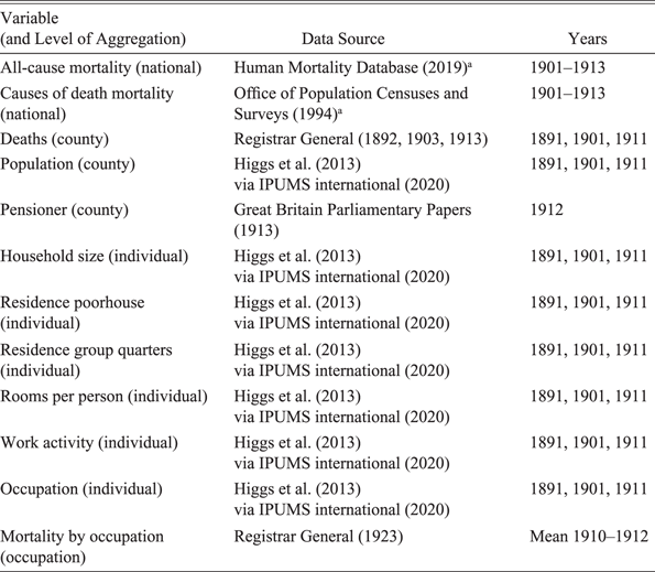
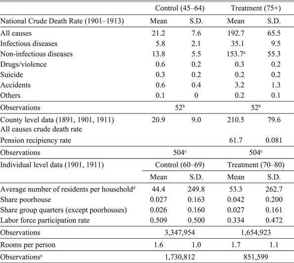
To study the impact of pensions on health, we use national-, regional-, and individual-level data for England and Wales. We rely on England and Wales for two reasons. First, age information is more reliable in England and Wales since birth registers (and birth certificates) have existed at least since 1837. In contrast, age verification was more difficult in Scotland and especially challenging in Ireland. Second, digitized individual-level census data, which we use to investigate the mechanism through which the pension affected mortality, is only consistently available for England and Wales. The national mortality sample starts in 1901 when the data from the Office of Population Censuses and Surveys (1994) (which provides us with cause of death data) begins and ends in 1913 due to the potential confounding mortality implications of WWI. Mortality data for England and Wales at the time can be considered to be of high quality and has been frequently used for empirical analyses (see, for instance, Beach and Hanlon 2018; Cummins Reference Cummins2021; Hanlon, Hansen, and Kantor 2021). Table 1 summarizes the variables and data sources of the study. Table 2 provides summary statistics. We group deaths into six different causes of death categories (based on more than 400 individual causes). Based on the death certificates at the time, most elderly people died due to old age (or senile decay),Footnote 21 which we include in the non-infectious disease category, followed by bronchitis, which is coded as an infectious disease. Together, old age and bronchitis make up almost half of all elderly deaths. Drug and violence-related deaths mostly include liver cirrhosis (as a proxy for alcoholism) and, to a smaller degree, homicides. Accident-related deaths are overwhelmingly caused by falls, and “Others” mostly consist of ill-defined or not specified deaths.
DATA SOURCES

Table 1 Long description
A table with 11 rows and 3 columns. The columns are labeled Variable (and Level of Aggregation), Data Source, and Years. The table summarizes the variables and data sources used in the study. Row 1: All-cause mortality (national), Human Mortality Database (2019), 1901-1913. Row 2: Causes of death mortality (national), Office of Population Censuses and Surveys (1994), 1901-1913. Row 3: Deaths (county), Registrar General (1892, 1903, 1913), 1891, 1901, 1911. Row 4: Population (county), Higgs et al. (2013) via IPUMS international (2020), 1891, 1901, 1911. Row 5: Pensioner (county), Great Britain Parliamentary Papers (1913), 1912. Row 6: Household size (individual), Higgs et al. (2013) via IPUMS international (2020), 1891, 1901, 1911. Row 7: Residence poorhouse (individual), Higgs et al. (2013) via IPUMS international (2020), 1891, 1901, 1911. Row 8: Residence group quarters (individual), Higgs et al. (2013) via IPUMS international (2020), 1891, 1901, 1911. Row 9: Rooms per person (individual), Higgs et al. (2013) via IPUMS international (2020), 1891, 1901, 1911. Row 10: Work activity (individual), Higgs et al. (2013) via IPUMS international (2020), 1891, 1901, 1911. Row 11: Occupation (individual), Higgs et al. (2013) via IPUMS international (2020), 1891, 1901, 1911. Row 12: Mortality by occupation (occupation), Registrar General (1923), Mean 1910-1912.
Source: a Underlying data from Registrar General.
To analyze the relationship between pension eligibility and health, we compare mortality rates above and below the newly created eligibility age of 70 in a difference-in-difference (DiD) and event-time framework using data at the national level from 1901 to 1913. The resulting estimates might not necessarily represent the causal effect of the pension on mortality; however, we argue in the Online Appendix that plausible confounders (e.g., spillover effects) are unlikely to invalidate our main results (Jaeger and Schacht-Picozzi Reference Jaeger and Schacht-Picozzi2025). People aged 75+ (age groups: 75–84, 85+) are coded as treated, while 45- to 64-year-olds (age groups: 45–54, 55–64) serve as a control. We use a narrower age definition as a robustness check. Since mortality data is only available in ten-year age brackets in official statistics, we drop the age group 65–74 because we cannot separate treated from non-treated.Footnote 22
On the national level, we run the following DiD:
 $$Detrended \, \log \left( {mortalit{y_{agt}}} \right) = \alpha \left( {eligibl{e_a}} \right) + {\beta _t}{\rm{\;}} + \gamma \left( {eligibl{e_a} \ge {\rm{\;}}{{1909}_t}} \right) + {\varepsilon _{agt}}$$
and event-time model:
 $$Detrended \, \log \left( {mortalit{y_{agt}}} \right) = \alpha \left( {eligibl{e_a}} \right) + {\beta _t} + \mathop \sum \limits_{k = 1901}^{1913} {\gamma _k}\left( {eligibl{e_a}{\rm{*\;}}yea{r_t}} \right) + {\varepsilon _{agt}}$$
where a denotes age-group, g gender, and t calendar time in years; eligible equals one for the age groups 75+ and zero otherwise, ≥ 1909
t
is one from 1909 onward and zero before; β
t
denotes time fixed effects. We are interested in the estimated DiD (
 $\widehat \gamma $
) and event-time coefficients (
 $\widehat {{\gamma _{\rm{k}}}}$
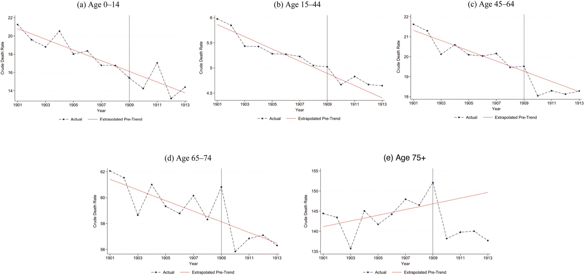
).We estimate Equations (1) and (2) using all-cause mortality as well as by different causes of death. Mortality is measured using the crude death rate, which divides the number of deaths by the size of the population in the respective year. Pre-pension mortality trends differed between our treated and control groups (see Figure 1). To account for that, we detrend mortality by regressing log(mortality) on age-group- and gender-specific linear time trends (and their interactions) in the pre-treatment period (1901–1908) and subtract these fitted trends from all data points (1901–1913) in the spirit of Bhuller et al. (Reference Bhuller, Havnes, Leuven and Mogstad2013) and Goodman-Bacon (Reference Goodman-Bacon2021). The detrending accounts for factors that influence mortality linearly over time but vary between groups, ensuring they do not bias our results. Time-fixed effects control for factors, regardless of their functional form, that affect mortality uniformly across age groups. Consequently, our estimation strategy is only potentially biased by mortality drivers with distinct effects across both time and age groups. These factors are discussed further in the next section.
MORTALITY TRENDS BY AGE, 1901–1913
Notes: Graphs show crude death rates for different age groups and a linear trend estimated based on the period from 1901 to 1908. The vertical line indicates the introduction of old-age assistance in 1909.
Source: Human Mortality Database (2019).

Different Pre-Trends
Notwithstanding the different pre-trends,Footnote 23 we argue that the identifying assumption—namely, that mortality rates would have continued on their pre-treatment trends in the absence of the pension—is valid. While inherently untestable, the assumption would be violated by any pension-unrelated factor or event that could account for the divergent trend in elderly mortality observed before 1909. However, we find no evidence of this. Instead, our findings indicate that a poorly designed social security system contributed to elevated elderly mortality prior to the reform. As the pension reform improved that system, one can assume that, without the pension, the rise in elderly mortality would have persisted beyond 1909.
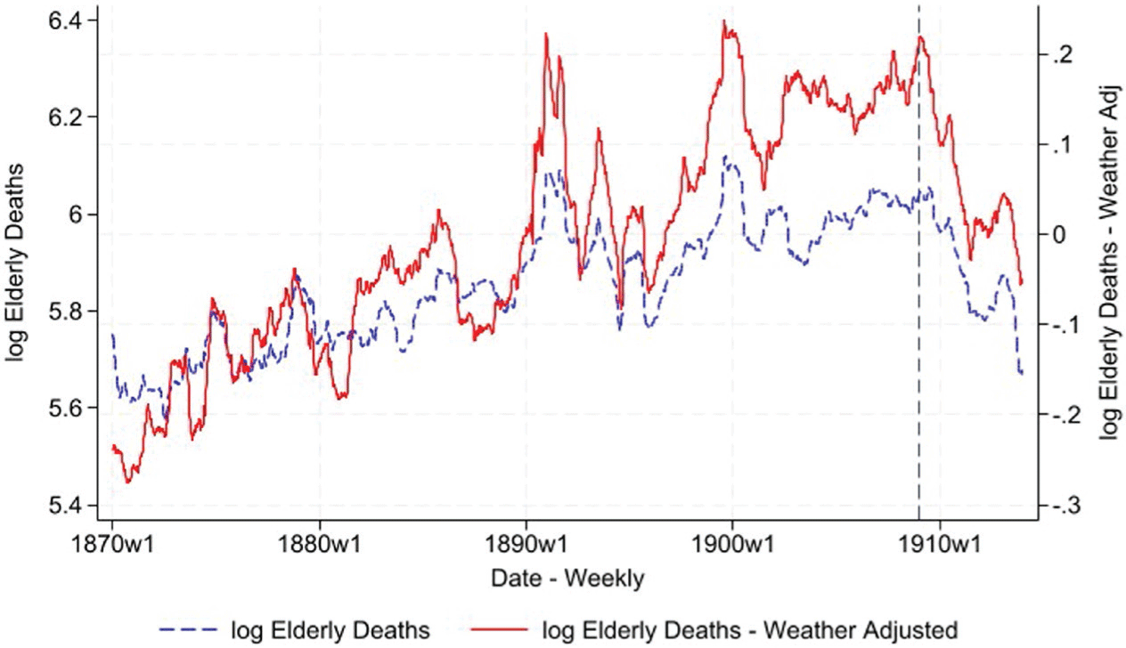
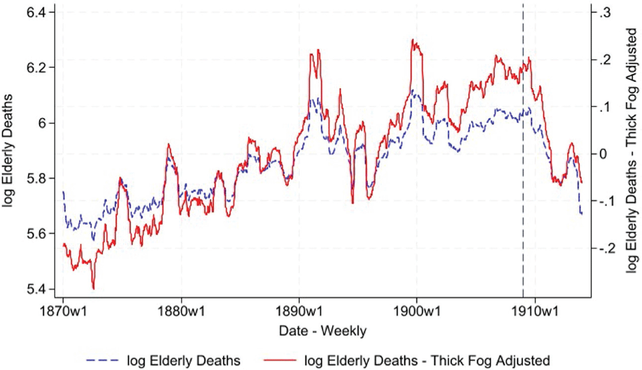
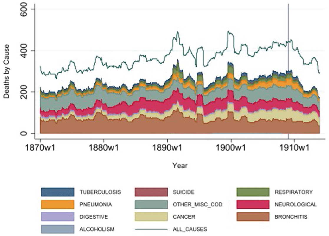
We first rule out pension-unrelated mortality drivers suggested in the previous literature as potential explanations for the observed elderly mortality trend (break). Hanlon, Hansen, and Kantor (2021) found that cold weather significantly increases elderly mortality in our period of interest. We use the data provided by Hanlon, Hansen, and Kantor (2021) to adjust weekly elderly deaths in London from 1870 to 1913 for weather effects in Figure 2. Our results show that weather was neither responsible for the increase in elderly mortality before 1909 nor for the decrease after 1909. Another important factor that elevated elderly mortality in our period of interest was pollution, as shown by Hanlon (Reference Hanlon2024b). We replicate Hanlon (Reference Hanlon2024b)’s empirical exercise by using thick fog weather events as a proxy for air pollution. Figure 3 shows that pollution-adjusted elderly mortality followed the same trend around the introduction of the pension. This makes sense since fog levels, indicative of pollution, were generally low in the early twentieth century (compare Hanlon Reference Hanlon2024b, fig. 11).Footnote 24 The London data also confirms our later finding that mortality changes are driven by many different causes of death and disease (compare Figure 4). A nationwide epidemic that coincidentally raised elderly mortality before 1909 is, therefore, unlikely. Online Appendix Figures E.1 and E.2 show stable consumer prices and steadily rising earnings per capita and consumption throughout our period of interest, suggesting no evidence of a nationwide economic downturn that adversely affected the elderly (e.g., due to food shortage). On the contrary, the period spanned an economic upswing, from which the elderly poor presumably did not benefit as they had not been able to accumulate sufficient retirement savings and were therefore heavily dependent on social assistance (Pugh Reference Pugh2002).Footnote 25
WEATHER ADJUSTED ELDERLY DEATHS IN LONDON
Notes: The blue line represents the weekly log of elderly deaths in London from 1870 until 1913. The red line depicts the residuals from regressing log of elderly deaths on various weather variables, including the number of days with temperatures below zero, rainfall amount, and very cold days, each with up to four lags and robust standard errors. Due to the pronounced seasonality in the raw data, the numbers are smoothed using a one-year moving average.
Source: Weekly mortality and weather data from Hanlon, Hansen, and Kantor (2021).

POLLUTION ADJUSTED ELDERLY DEATHS IN LONDON
Notes: The blue line represents the weekly log of elderly deaths in London from 1870 until 1913. The red line shows the residual from regressing log elderly deaths on days with thick fog in the current week and the two previous weeks, with robust standard errors. Due to pronounced seasonality in the raw data, the numbers are smoothed using a one-year moving average.
Source: Weekly mortality and weather data from Hanlon, Hansen, and Kantor (2021).

CAUSES OF DEATH LONDON
Notes: All time series are depicted as yearly moving averages. The ten most important sources of death as area graphs, stacked on top of each other.
Source: Weekly mortality and weather data from Hanlon, Hansen, and Kantor (2021).

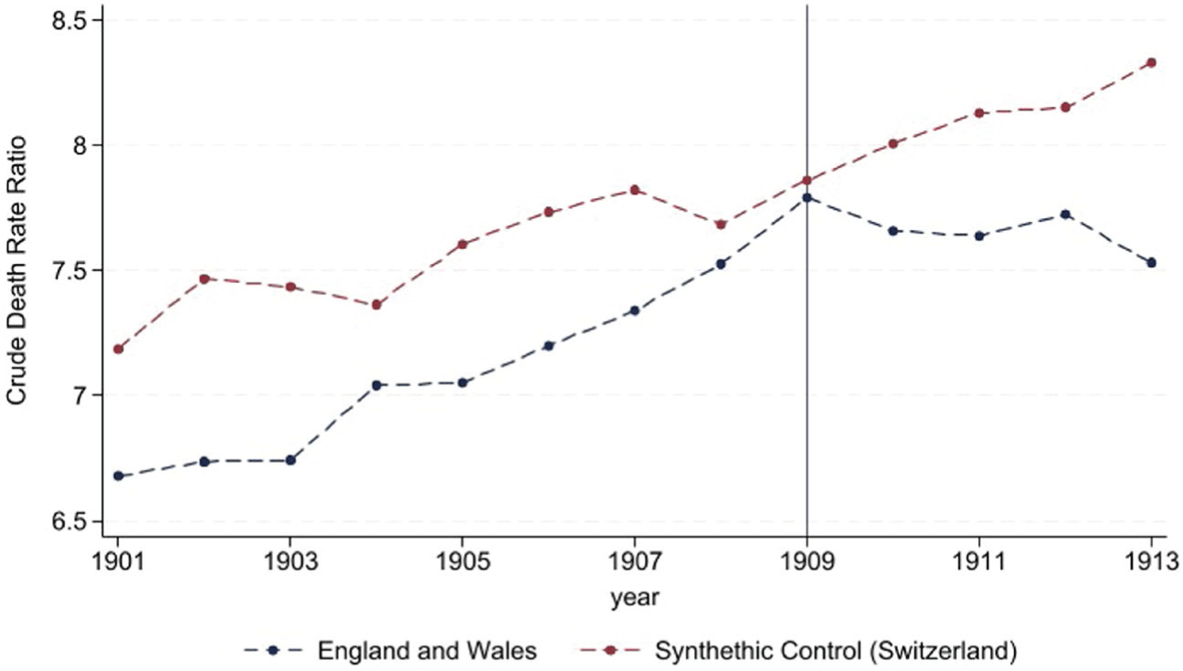
Instead of pension-unrelated factors, historical literature suggests that deficiencies in the social security system contributed to the deteriorating living conditions of the elderly prior to the pension reform (Boyer Reference Boyer2019). In the decades before the pension, Poor Law provisions had become increasingly restrictive and conditional on living in poorhouses—a major policy shift now known as the “Crusade Against Outrelief” (MacKinnon Reference MacKinnon1987; Thomson Reference Thomson1983). These poorhouses were notorious for their harsh living conditions and social stigma, which deterred many elderly from seeking financial assistance (Crowther Reference Crowther1981). As a result, most elderly men continued to work in low-skilled and hazardous jobs. On this basis, we argue that without the pension reform, the deterioration in the living conditions of the elderly and the increase in elderly mortality would likely have continued. This assumption is supported by a synthetic control group approach, comparing England and Wales to a range of potentially similar countries for which data is available at the time in the Human Mortality Database (2019) (Finland, Italy, Netherlands, Norway, Sweden, and Switzerland). Figure 5 shows that elderly mortality (relative to middle-aged mortality) did not decline in synthetic England and Wales after the pension was implemented. Although the informational content of the exercise should not be overstated (as the algorithm selects Switzerland as the sole component of synthetic England and Wales), the overall evidence supports the assumption that attributes the trend break in elderly mortality to the pension reform.
MORTALITY RATIO TREATED VS. CONTROL, ENGLAND AND WALES VS. SYNTHETIC CONTROL
Notes: Crude death rate of the elderly (75+) divided by the crude death rate of the middle-aged (45–64). Donor pool for the synthetic control: Finland, Italy, Netherlands, Norway, Sweden, and Switzerland. The vertical line indicates the introduction of old-age assistance in 1909 in the United Kingdom.
Source: Human Mortality Database (2019).

Results
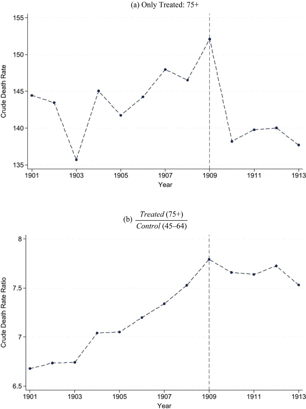
We argue in this section that the introduction of public pensions in the United Kingdom reduced elderly mortality. Purely descriptively, Figure 6 documents a trend break in elderly mortality rates after the pension was introduced. Both, the crude death rates (deaths per 1,000 people) of the treatment group (top panel) and the ratio of crude death rates between treatment and control (bottom panel) show an increase in elderly mortality (absolute or relative to middle-aged mortality) before the pension became effective in 1909. After 1909, elderly mortality declined. We document in Figure 1 that there is no evidence of a trend break in mortality rates after 1909 for any other age group, all of which hints at a pension-induced reduction in elderly mortality.Footnote 26
MORTALITY RATES IN ENGLAND AND WALES, 1901–1913
Notes: Top panel: Crude death rates of the treatment group calculated as
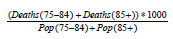 $\frac{{\left( {Deaths\left( {75 - 84} \right) + Deaths\left( {85 + } \right)} \right)*1000}}{{Pop\left( {75 - 84} \right) + Pop\left( {85 + } \right)}}$
. Bottom panel: Crude death rate of the treatment group divided by the crude death rate of the control group
 $\frac{{\left( {Deaths\left( {45 - 54} \right) + Deaths\left( {55 - 64} \right)} \right)*1000}}{{Pop\left( {45 - 54} \right) + Pop\left( {55 - 64} \right)}}$
. The vertical line indicates the introduction of old-age assistance in 1909.
Source: Human Mortality Database (2019).

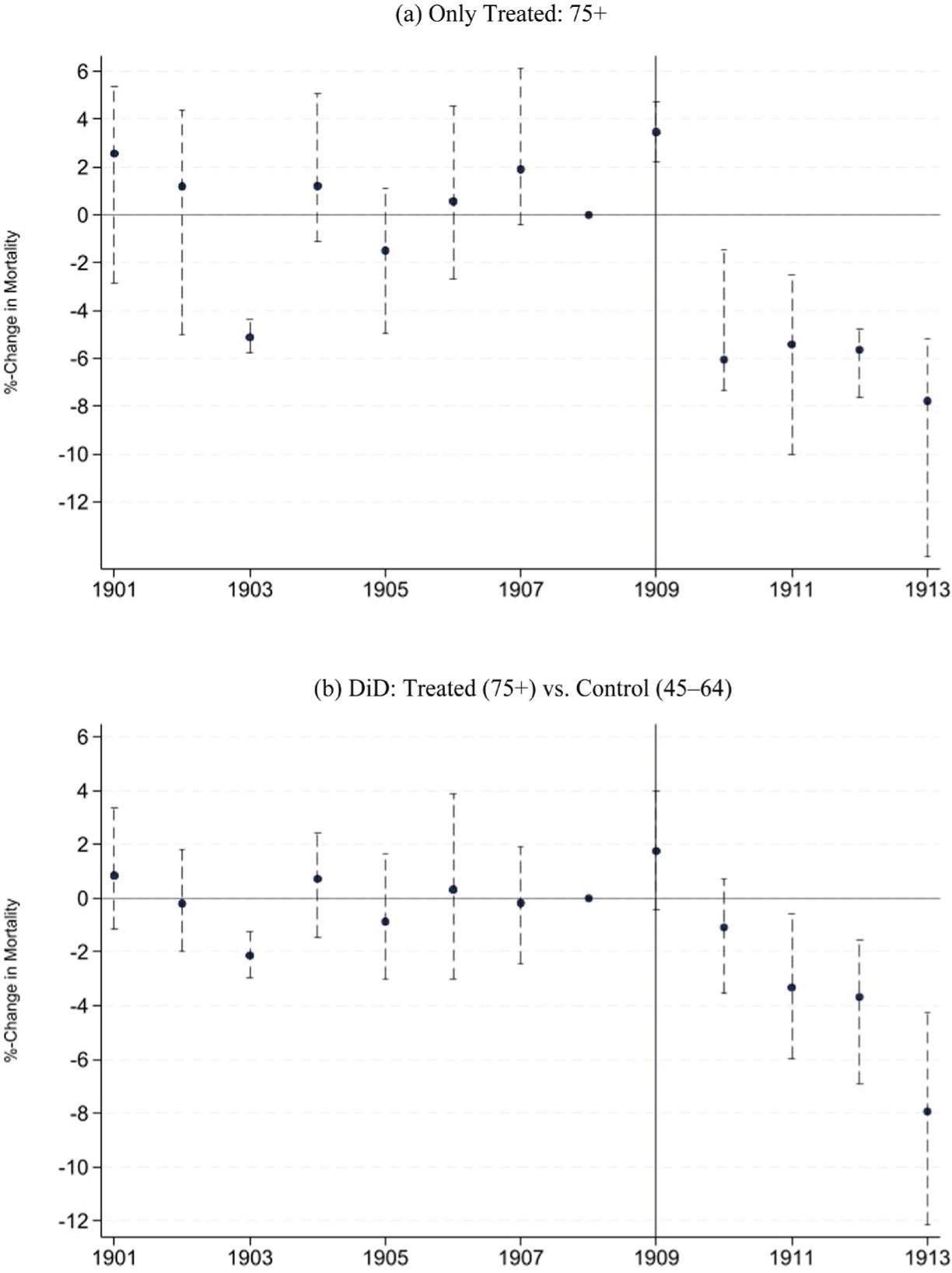
Figure 7 illustrates the key takeaway of Figure 6 using a more formal event-time model. Assuming that the pre-pension trends would have continued in the absence of the pension, elderly mortality would have been almost 8 percent lower in 1913 compared to 1908. Contrasting the entire post-reform period (1909–1913) with the pre-treatment period (1901–1908), detrended elderly mortality fell on average by 2.7 percent (Table 3) after the pension was introduced. These estimates are consistent with an economically relevant health benefit of the pension.Footnote 27
PENSION AND MORTALITY: NATIONAL EVENT-TIME MODEL
Notes: Coefficients (and 95 percent confidence bands) from an event-time model. Only treated: year dummies, DiD: Interaction of year and treatment dummy (1 if age ≥70), both 1908 baseline year. Dependent variable: detrended ln(mortality rates). The vertical line indicates the introduction of old-age assistance in 1909. Standard errors clustered at the age-group-gender level using wild-bootstrap and Webb weights.
Source: Human Mortality Database (2019).

Figure 7 Long description
The image contains two line graphs. Panel A shows the percent change in mortality for the age group 75 and older from 1901 to 1913. The x-axis represents the years, and the y-axis represents the percent change in mortality. The data points are marked with dots, and error bars indicate the 95 percent confidence intervals. The vertical line at 1909 indicates the introduction of old-age assistance. Panel B shows the difference-in-differences (DiD) analysis comparing the percent change in mortality for the treated group (age 75 and older) versus the control group (ages 45 to 64) over the same period. The x-axis represents the years, and the y-axis represents the percent change in mortality. The data points are marked with dots, and error bars indicate the 95 percent confidence intervals. The vertical line at 1909 indicates the introduction of old-age assistance. Both graphs show the impact of old-age assistance on mortality rates, with a focus on the changes before and after 1909.
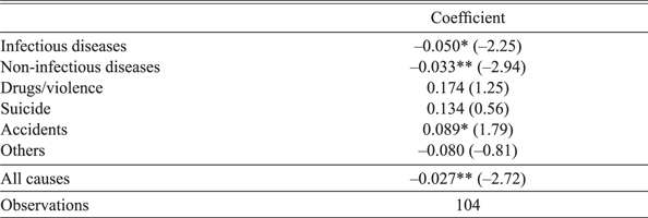
Turning to causes of death shows that mortality from infectious as well as non-infectious diseases declined after the pension was introduced (Table 3). The decline was strongest for infectious diseases, which aligns with the hypothesis that the pension reduced crowding by making it less likely to contract an infection. Deaths from non-infectious diseases also declined, which is consistent with the idea that the pension allowed people to retire from jobs characterized by hard manual labor or hazardous workplaces. We find no statistically significant change in mortality related to risky behavior such as drug abuse and violence (mainly alcoholism and homicides) or social isolation (proxied by suicides in the spirit of Stoian and Fishback Reference Stoian and Fishback2010), which might at least partly be driven by too much statistical noise due to the relatively low number of deaths associated with these causes of death (Table 2). The rather surprising finding that accident-related mortality increased after the pension was introduced could be driven by the possibility that a reduction in work-related accidents is overcompensated by accidents at home (which we cannot disentangle in the data). Another potential explanation is that the pension allowed elderly people to live in private households,Footnote 28 instead of being monitored in a poorhouse or other collective institutions, which might have increased the risk of accidents.
SUMMARY STATISTICS

Table 2 Long description
A table comparing summary statistics for control and treatment groups across various categories. The table has 21 rows and 8 columns. Column headers are Control (45-64), Treatment (75+), and County level data (1891, 1901, 1911). Row labels include National Crude Death Rate (1901-1913), Infectious diseases, Non-infectious diseases, Drugs/violence, Suicide, Accidents, Others, Observations, All causes crude death rate, Pension recipiency rate, Average number of residents per household, Share poorhouse, Share group quarters (except poorhouses), Labor force participation rate, Rooms per person, and Observations. The table presents mean and standard deviation (S.D.) values for each category. For example, under National Crude Death Rate (1901-1913), the mean for All causes in the Control group is 21.2 with an S.D. of 7.6, while in the Treatment group, the mean is 192.7 with an S.D. of 65.5. The table also includes observations for County level data and Individual level data. Notable trends include higher death rates and pension recipiency rates in the Treatment group compared to the Control group.
Notes: Crude death rates (deaths per 1,000 people) are unweighted averages for the age-groups used in the estimation, for example, the mean of the all cause crude death rate is the unweighted average of the death rate for people aged 75–84 (129.5) and 85+ (255.9). In contrast, Figure 6 shows weighted averages. a = Note that the majority of non-infectious disease deaths in the 75+ population were attributed to vague causes of old age (variables named old age, senile decay, and syncope [indicative of unspecified heart diseases]). According to Reid et al. (Reference Reid, Garrett, Dibben and Williamson2015), those causes likely indicate a lack of precise diagnosis rather than specific diseases as causes of death. b = 2 age-groups * 2 genders * 13 years. c = 2 age-groups * 2 genders * 3 years * 42 counties. d = Average number of residents per household is high due to people living in group quarters with thousands of other persons. Those individuals receive greater weight in this calculation than they would in a standard household-size average. The median household size for the control group is 4 and 3 for the treatment group. e = number of rooms is missing for some households (mostly group quarters).
Source: See Table 1.
PENSION AND MORTALITY: NATIONAL DiD-ESTIMATES

Table 3 Long description
A table with 8 rows and 3 columns. The columns are labeled Cause and Coefficient. The rows are labeled Infectious diseases, Non-infectious diseases, Drugs/violence, Suicide, Accidents, Others, All causes, and Observations. The table presents coefficients and their corresponding t-values for different causes of mortality. Infectious diseases have a coefficient of -0.050 with a t-value of -2.25. Non-infectious diseases have a coefficient of -0.033 with a t-value of -2.94. Drugs/violence have a coefficient of 0.174 with a t-value of 1.25. Suicide has a coefficient of 0.134 with a t-value of 0.56. Accidents have a coefficient of 0.089 with a t-value of 1.79. Others have a coefficient of -0.080 with a t-value of -0.81. All causes have a coefficient of -0.027 with a t-value of -2.72. Observations are listed as 104.
* = Significant at the 10 percent level.
** = Significant at the 5 percent level.
Notes: Coefficients from a difference-in-difference model (interaction of post-treatment-period and treatment dummy). Dependent variable: detrended ln(mortality rates). Treatment age-groups: 75+. Control age-groups: 45–64 years. Years 1901–1913. Other causes include deaths related to pregnancy or birth and deaths with unknown or ill-defined causes. Standard errors clustered at the age-group level using wild-bootstrap and Webb weights. t-value in parentheses.
Source: See Table 1.
PENSION AND MORTALITY: COUNTY LEVEL ESTIMATES

Table 4 Long description
A table comparing treatment intensity and mortality rates across different years. The table has two rows and three columns. The columns are labeled Coefficient, Observations, and Treatment intensity. The rows are labeled Treatment intensity in 1911 and Treatment intensity in 1891. The table shows the coefficient values and observations for each treatment intensity. For Treatment intensity in 1911, the coefficient is -0.245 with a standard error of 0.144, and there are 1,008 observations. For Treatment intensity in 1891, the coefficient is -0.043 with a standard error of 0.219, and there are 1,008 observations. The table also includes a note indicating that the coefficient of the triple interaction (eligible a * year t * pension rate c) is shown, with the dependent variable being the natural logarithm of mortality rates. The treatment age-groups are 75+, and the control age-groups are 45-64. The sample consists of the census years 1891, 1901, and 1911, with 1901 as the base year of the interactions. Standard errors are clustered at the county level.
* = Significant at the 10 percent level.
Notes: Coefficient of the triple interaction ρ (eligible a * year t * pension rate c ). Dependent variable: ln(mortality rates). Treatment age-groups: 75+. Control age-groups: 45–64. Sample consists of the census years 1891, 1901, 1911. Base year of the interactions: 1901. Standard errors (in parentheses) are clustered at the county level.
Source: See Table 1.
COUNTY LEVEL ANALYSIS
Data and Identification Strategy
To investigate whether the treatment intensity is associated with changes in mortality rates, we exploit variations in pension recipient rates at the country level. We use data from the three census years 1891, 1901, and 1911 and consider only the 42 English counties, because county-level mortality information is not consistently reported for Welsh counties over the three decades.Footnote 29 As in our national level analysis, people aged 75+ (age groups: 75–84, 85+) are coded as treated while 45-to-64-year old’s (age groups: 45–54, 55–64) serve as a control. We run a triple interaction model of the following form:
 $$\matrix{ {log\left( {mortalit{y_{agtc}}} \right) = \alpha \left( {eligibl{e_a}} \right) + {\beta _t} + \gamma \left( {pension\,rat{e_c}} \right)} \hfill \cr {\,\,\, + {\delta _t}\left( {eligibl{e_a}*yea{r_t}} \right) + \lambda \left( {eligibl{e_a}*pension\,rat{e_c}} \right)} \hfill \cr { + {\mu _t}\left( {yea{r_t}*pension\,rat{e_c}} \right) + {\rho _t}\left( {eligibl{e_a}*yea{r_t}*pension\,rat{e_c}} \right) + {\varepsilon _{agtc}}} \hfill \cr }$$
where a denotes age-group, g gender, t calendar time in years, and c county; eligible, as in Equations (1) and (2), equals one for the age groups 75+, and zero otherwise; pensionrate
c
is the share of pensioners relative to the elderly population (70+) and serves as a proxy for the treatment intensity at the regional level. We do not detrend mortality, which would be challenging with two pre-reform data points, and instead focus solely on the estimated triple interaction coefficient
 ${\widehat \rho _{1911}}$
.
Results
The county-level estimates presented in Table 4 support the national-level finding that the introduction of pensions was associated with a decline in elderly mortality. The coefficient of the triple interaction (
 ${\widehat \rho _{1911}}$
of Equation (3)) is negative and statistically significant at the 10 percent level, which suggests that elderly (relative to middle-aged) mortality declined more strongly in counties with a higher treatment intensity. The estimated coefficient of –0.245 implies that an increase in the recipiency rate from 0 to 57.5 percent (the national recipiency rate in 1911) is associated with a mortality decline of 12.5 percent. Thus, the county-level estimates suggest an even stronger positive health effect of the pension than the national DiD analysis. The coefficient
 ${\widehat \rho _{1891}}$
of the interaction of eligible
a
* (Year = 1891)
t
* (pensionrate)
c
is negative and insignificant, indicating that the result is not driven by pre-existing trends.
INDIVIDUAL LEVEL ANALYSIS - MECHANISMS
Data and Identification Strategy
The individual-level analysis relies on full-count census data for up to three decennial waves (1891, 1901, 1911). Online Appendix Figure E.3 shows the number of observations for every age between 50 and 90 for the two censuses used in the main analysis (1901, 1911). We analyze two potential transmission channels, crowding and retirement, in a difference-in-difference design. To identify the causal effect of pension availability on housing arrangements and labor supply, we take advantage of the more granular microdata, which allows us to compare people slightly above with people slightly below the newly created pension eligibility age.
Specifically, we estimate for every age between 60 and 80 a 2×2 DiD equation of the following form:
 $${y_{at}} = \alpha \left( {ag{e_a}} \right){\rm{ }} + \beta \left( {year = {\rm{ }}{{1911}_t}} \right){\rm{ }} + \gamma \left( {ag{e_a}*{\rm{ }}year{\rm{ }} = {\rm{ }}{{1911}_t}} \right){\rm{ }} + {\varepsilon _{at}}$$
where age 69 always serves as a reference group, and the regression is estimated for the census wave t 1901 (before) and 1911 (after). The coefficients of primary interest, γ, measure the percentage-point change in the outcome variable (between 1901 and 1911) of the ages 60 to 80 compared to the reference age of 69. The identifying assumption is that people slightly below or above the age of 69 would have behaved like people aged 69 without the pension. We discuss potential threats to identification and why they are unlikely to apply in the Online Appendix. Using graphical DiD evidence for the age groups 75+ and 45–64, we investigate whether the estimated local DiD also has implications for the age groups studied in the mortality analysis.
We use three main variables to operationalize crowding: First, the average number of residents per household;Footnote 30 second, the share of people living in collective dwellings such as poorhouses; and third, the number of rooms per person. To study retirement patterns, we follow Giesecke and Jäger (Reference Giesecke and Jäger2021) and use labor force participation (LFP) rates derived by the gainful employment concept as the main outcome.Footnote 31 We estimate the LFP-DiD for four different occupational groups based on their occupation-specific mortality rates.
Results
RESIDENTIAL CROWDING
One channel through which the pension likely decreased mortality is by reducing residential crowding, thus impeding the spread of infectious diseases and, to a lesser extent, improving the prospects for recovery from grueling non-infectious diseases. Previous studies have shown that crowding was associated with higher mortality rates at the time in both the United Kingdom (Hanlon and Tian 2015) and the United States (Ager et al. Reference Ager, Feigenbaum, Hansen and Ren Tan2024). We confirm the positive and statistically significant correlation between crowding and mortality in the United Kingdom at the time by running a simple bivariate regression at the district level of elderly mortality rates (75+) on our main proxy for household crowding, the average number of residents per householdFootnote 32 (results see Table D.1 in the Online Appendix).
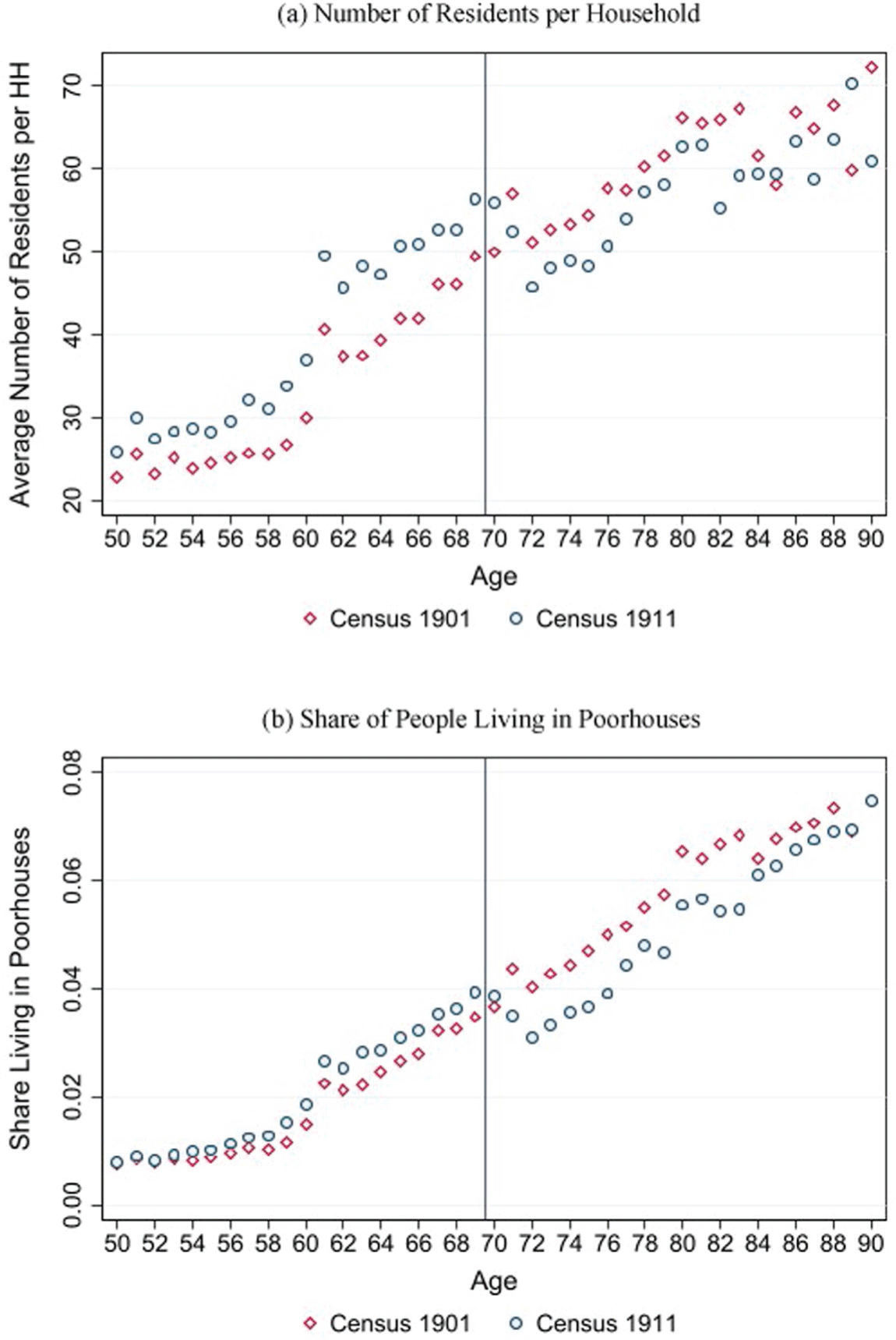
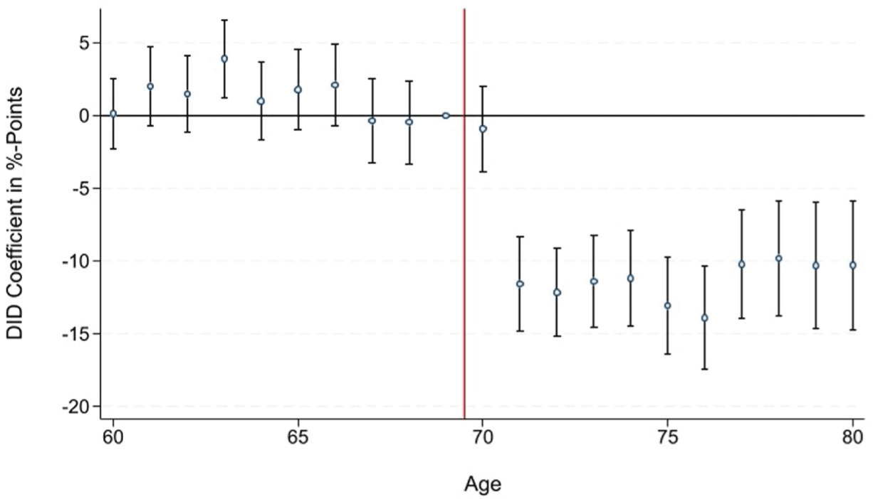
Consistent with historical evidence from the United States (Costa Reference Costa1997, Reference Costa1999), we argue in this section that the introduction of public pensions in the United Kingdom altered living arrangements. The top panel of Figure 8 shows descriptively that the average number of residents per household declined at the newly introduced eligibility age after the pension was introduced (1911), while it used to increase before the pension was available (1901). Figure 9, plotting 20 2×2 DiD coefficients, shows the argument more formally. While the average number of residents per household of people aged 60 to 69 moved in tandem between 1901 and 1911, the average number of residents per household for people aged 70+ decreased significantly relative to people aged 69. The estimated decline in the number of residents per household to up to 14 people is economically relevant, given that it implies a reduction of the average number of residents per household of more than 20 percent compared to 1901. A placebo test, presented in Online Appendix Figure E.4, documents that the average number of residents per household for people 70+ has mostly evolved like the average number of residents per household for people aged 69 in the pre-treatment period (between 1891 and 1901). The reduction in crowding that took place only after the introduction of pensions is also visible for the larger treatment group (75+) used in the mortality estimates (Online Appendix Figure E.5), especially when compared to the mortality control group (45–64).
NUMBER OF RESIDENTS PER HOUSEHOLD AND SHARE OF PEOPLE LIVING IN POORHOUSES, 1901 AND 1911
Note: The vertical line indicates the age-based eligibility threshold that was introduced by the pension in 1909.
Source: Own calculations based on individual full-count census data for England and Wales provided by IPUMS.

Figure 8 Long description
Two line graphs depict the number of residents per household and the share of people living in poorhouses in 1901 and 1911. Panel A: The line graph shows the average number of residents per household against age. The x-axis represents age, ranging from 50 to 90 years, and the y-axis represents the average number of residents per household, ranging from 20 to 70. Two data series are plotted: one for Census 1901 (red diamonds) and one for Census 1911 (blue circles). The graph indicates an increasing trend in the average number of residents per household with age for both censuses, with a noticeable rise after age 70. Panel B: The line graph shows the share of people living in poorhouses against age. The x-axis represents age, ranging from 50 to 90 years, and the y-axis represents the share living in poorhouses, ranging from 0.00 to 0.08. Two data series are plotted: one for Census 1901 (red diamonds) and one for Census 1911 (blue circles). The graph indicates an increasing trend in the share of people living in poorhouses with age for both censuses, with a noticeable rise after age 70. The vertical line in both graphs indicates the age-based eligibility threshold introduced by the pension in 1909.
DIFFERENCES-IN-DIFFERENCES ESTIMATES FOR NUMBER OF RESIDENTS PER HOUSEHOLD
Notes: Each dot represents a 2×2 difference-in-difference coefficient (and 95 percent confidence bands) comparing the change in number of residents per household between 1901 (before) and 1911 (after) for each age (60–80) relative to the reference age 69. The vertical line indicates the age-based eligibility threshold that was introduced by the pension in 1909.
Source: Own calculations based on individual full-count census data for England and Wales provided by IPUMS.

The decline in the number of residents per household is mostly driven by fewer people residing in poorhouses or other collective dwellings and living in private households instead. Collective dwellings, also known as group quarters, include, among others, correctional institutions, hospitals, military barracks, boarding schools, convents, and most importantly in this setting, poorhouses. Poor- or workhouses, based on the centuries-old Poor Law system, were institutions that offered accommodation and employment for people who were unable to support themselves financially. Footnote 33 The fact that the number of residents per household increases with age (as shown in the top panel of Figure 8) is mostly driven by elderly people who lose the capacity to work and move to a poorhouse to receive governmental support (bottom panel of Figure 8). Poorhouses were typically very crowded. Based on the census in 1911, elderly people (70+) in poorhouses lived together with, on average, 760 other people, while elderly people residing in private households, as more than 90 percent of them did, shared their home with, on average, three other people (see Online Appendix Figure E.6).
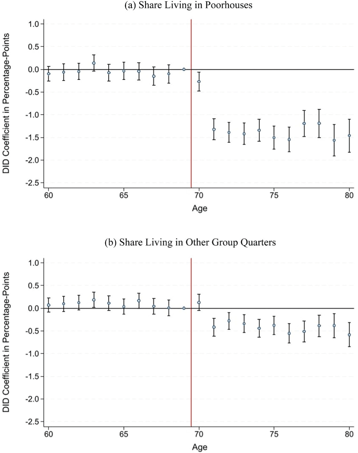
Figure 10, using the same DiD design as in Figure 9, indicates that both the share of people living in poorhouses and the share of people living in other group quarters declined after the pension was introduced. The decline, however, is much stronger for poorhouses and amounts to around 1.5 percentage points, implying a reduction of more than 30 percent compared to 1901. The finding of a substantial reduction in the share of people living in poorhouses is in line with administrative statistics showing that the absolute number of elderly people (70+) in poorhouses declined by almost 20 percent from March 1906 to January 1912 (from 61,378 to 49,370 according to Great Britain Parliamentary Papers (1913)). Our findings make sense because, in addition to providing recipients with greater financial means, the pension removed the need to live in a poorhouse in order to receive relief (MacKinnon Reference MacKinnon1987). The reduction in the overall number of elderly people in poorhouses facilitated their transformation into higher-quality nursing homes, which continued to house elderly individuals after the introduction of the pension while offering improved care (Thomson Reference Thomson1983). We find only limited evidence for a reduction in crowding conditional on living in a private household or group quarters (Online Appendix Figure E.7), which is likely driven by the fact that the composition (fewer people in group quarters, more in private households) changed at the newly created retirement age.
DIFFERENCES-IN-DIFFERENCES ESTIMATES FOR SHARE LIVING IN COLLECTIVE DWELLINGS
Notes: Each dot represents a 2×2 difference-in-difference coefficient (and 95 percent confidence bands) comparing the change in the share of people living in poorhouses (top panel) or group quarters except poorhouses (bottom panel) between 1901 (before) and 1911 (after) for each age (60–80) relative to the reference age 69. The vertical line indicates the age-based eligibility threshold that was introduced by the pension in 1909.
Source: Own calculations based on individual full-count census data for England and Wales provided by IPUMS.

Figure 10 Long description
Two line graphs depict the share of people living in collective dwellings, comparing changes between 1901 and 1911 for different ages relative to a reference age. Panel A: The top panel shows the share living in poorhouses. The x-axis represents age, ranging from 60 to 80, and the y-axis represents the DID coefficient in percentage points, ranging from -2.5 to 1.0. Each dot represents a difference-in-difference coefficient with 95 percent confidence bands. The vertical line at age 70 indicates the age-based eligibility threshold introduced by the pension in 1909. The data shows a significant drop in the share of people living in poorhouses after age 70. Panel B: The bottom panel shows the share living in other group quarters. The x-axis represents age, ranging from 60 to 80, and the y-axis represents the DID coefficient in percentage points, ranging from -2.5 to 1.0. Each dot represents a difference-in-difference coefficient with 95 percent confidence bands. The vertical line at age 70 indicates the age-based eligibility threshold introduced by the pension in 1909. The data shows a slight decrease in the share of people living in other group quarters after age 70.
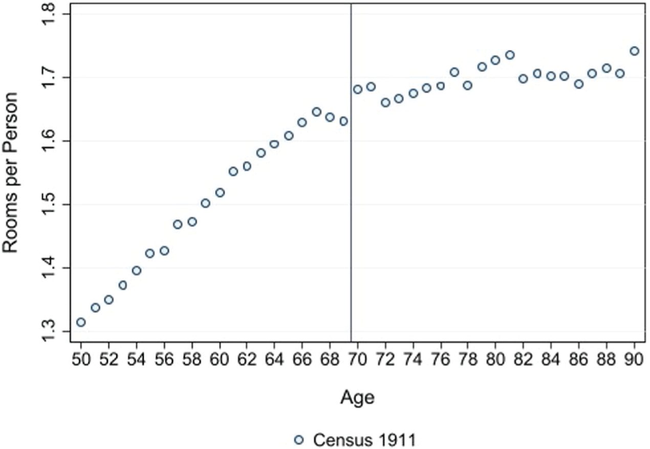
Looking at a more direct measure of household crowding—the average number of rooms per person—supports the previous findings. The number of rooms for a given household is only available for a large number of households since 1911; thus, estimating a DiD specification is not feasible. Figure 11, however, demonstrates a clear increase in the average number of rooms per person at age 70.Footnote 34 The visible increase is likely even downward-biased because the number of rooms is often missing for group quarters, which are typically more crowded than private households.Footnote 35
RETIREMENT FROM PHYSICALLY INTENSIVE OR HAZARDOUS JOBS
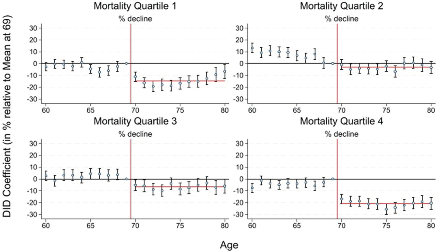
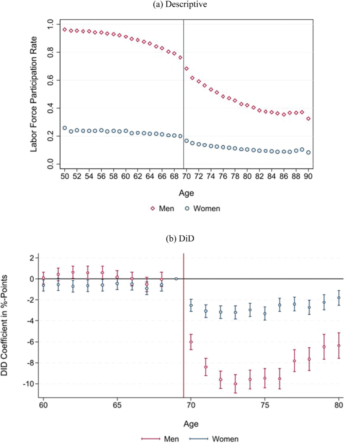
The second probable channel through which the pension reduced mortality is by enabling elderly people to retire from physically intensive or hazardous jobs. To document this, we estimate male labor supply responses depending on occupation-specific mortality rates. We focus on men because occupation-specific mortality rates are not available for women. Footnote 36 We group all men aged 60 to 80, which we could match to an occupation-specific mortality rate (70 percent of men with an occupation), in four (almost)Footnote 37 equally sized mortality groups. We then run 20 DiD models for each of the four sub-groups.Footnote 38 The mortality differences between the mortality quartiles are pronounced. Average occupational mortality in the lowest mortality quartile amounts to around 60 percent of average male mortality (for the same age group) and more than 200 percent in the highest mortality group.
Figure 12 shows that the decline in labor force participation rates, as estimated via a DiD design, is strongest in occupations with the highest occupational mortality rate. In the quartile with the highest mortality rates (quartile 4), male labor supply in the age group 70 to 80 declined by, on average, 20.9 percent compared to age 69. The majority of people in the highest mortality quartile were working in elementary occupations, mainly including general laborers. Retirement from elementary occupations, which were likely physically very demanding, stressful, and poorly paid, has plausibly contributed to a reduction in elderly mortality rates. The decline is smaller (ranging between 2.9 and 14.4 percent) in the groups with lower mortality rates. The large labor supply reduction in the first mortality quartile is driven by farmers, who had relatively low mortality rates, likely due to not being exposed to crowded cities with poor sanitary conditions. Given that agricultural work at the time was also physically intense, the finding of large labor supply responses in the first mortality quartile is not at odds with the general conclusion that the pension allowed people to retire from physically intensive jobs. Online Appendix Figure E.8 shows that elderly labor supply more generally, measured based on the larger treatment group (75+) as used in the mortality analysis, has shown a continued decrease in their labor market participation compared to the middle-aged (45–64).
ROOMS PER PERSON, 1911
Notes: Figure plots the average number of rooms in a household divided by the number of household members. The number of rooms is missing for many group quarters. The vertical line indicates the age-based eligibility threshold that was introduced by the pension in 1909.
Source: Own calculations based on individual full-count census data for England and Wales provided by IPUMS.

DIFFERENCES-IN-DIFFERENCES ESTIMATES FOR MALE LABOR SUPPLY STRATIFIED BY OCCUPATIONAL MORTALITY RATE
Notes: Each dot represents a 2×2 difference-in-difference coefficient (and 95 percent confidence bands) comparing the change in the share of people working in a job associated with a specific mortality quartile between 1901 (before) and 1911 (after) for each age (60–80) relative to the reference age 69. All estimates are scaled by the average share of people working in a job associated with the respective mortality quartile at age 69. The decline specified in the subtitles and represented by the red horizontal line measures the average coefficient for the ages 70 to 80. The vertical line indicates the age-based eligibility threshold that was introduced by the pension in 1909. Occupations ranked by average male mortality rate based on Registrar General (1923) 1. quartile: Lowest mortality rate, 4. quartile: Highest mortality rate.
Source: Own calculations based on individual full-count census data for England and Wales provided by IPUMS and Registrar General.

OTHER POTENTIAL CHANNELS
More or higher-quality nutrition also likely contributed to the mortality decline. The diet of poor people in the United Kingdom at the time was characterized by insufficient levels of vitamins and minerals (Gazeley and Newell Reference Gazeley and Newell2015), and a pension of five shillings could buy a considerable amount of food.Footnote 39 Due to the lack of data, we are unable to evaluate the contribution of nutrition empirically. The finding that the mortality decline was roughly similar for men and women, although men responded more in terms of crowding and labor supply, suggests that another channel, most likely nutrition, also played an important role.
Another potential mechanism is that the pension allowed elderly people to spend more on heating. We test this hypothesis using data from Hanlon, Hansen, and Kantor (2021), who provide weekly death counts by age, together with temperature data for London. Running a regression with the number of elderly deaths (aged 65+) as the dependent variable for the period from 1901 to 1913, we find that elderly mortality increases if the minimum temperature falls below 0 degrees Celsius. However, the temperature-mortality nexus does not change significantly after 1908, suggesting that additional spending on heating has played only a minor role (see Online Appendix Table D.2).
Improved medical care was probably also less relevant because medical technology was still limited. Although some vaccinations, for example, against smallpox, rabies, or the plague had already been invented, the mortality implications of these vaccines were likely limited (Cutler, Deaton, and Lleras-Muney Reference Cutler, Deaton and Lleras-Muney2006). Antibacterial medications such as sulfa drugs or penicillin were not widely used before the 1930s and 1940s. Effective treatment against diseases associated with old age, such as cancer or cardiovascular disease only, started to emerge after WWII.
HETEROGENEITY
Rural vs. Urban
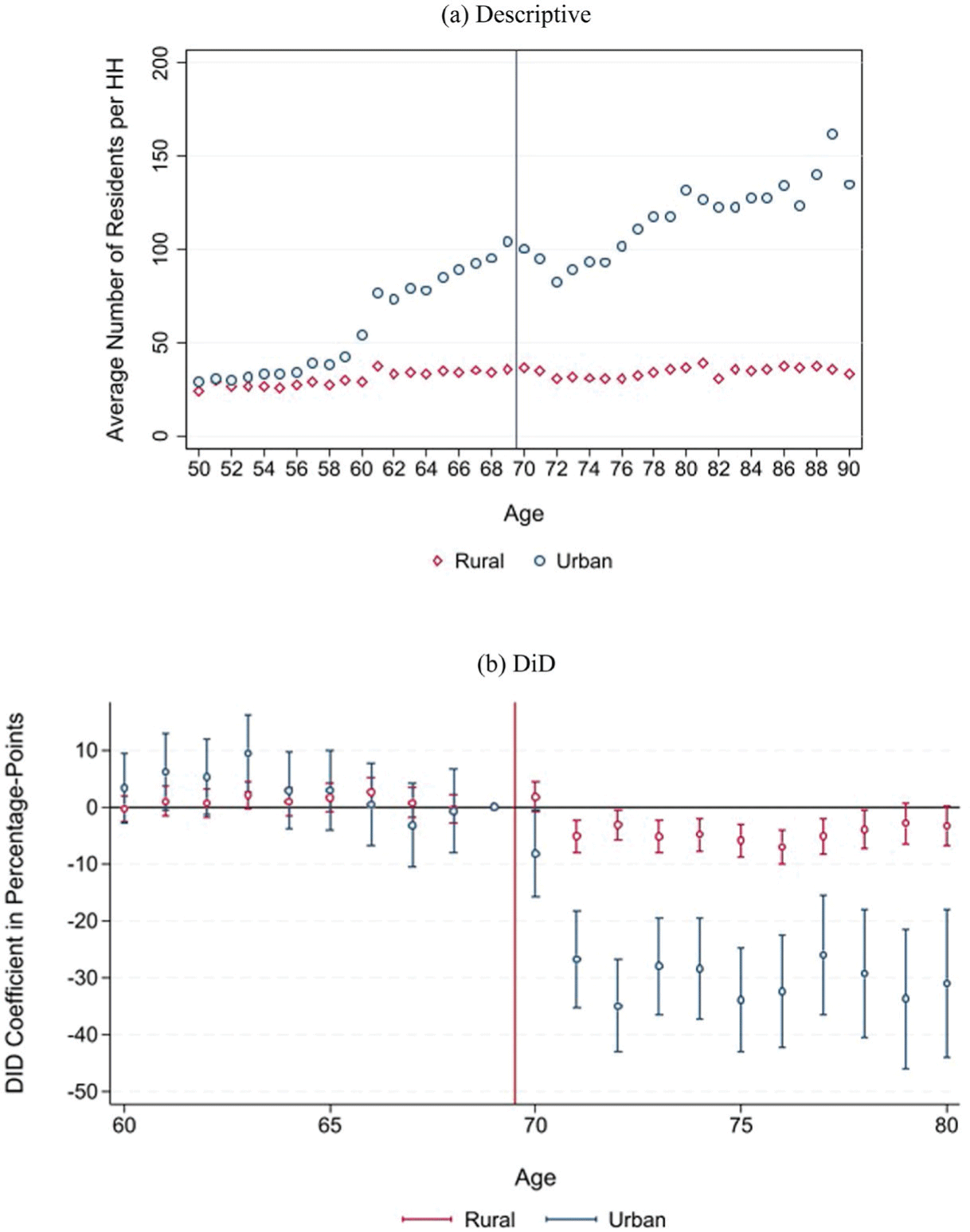
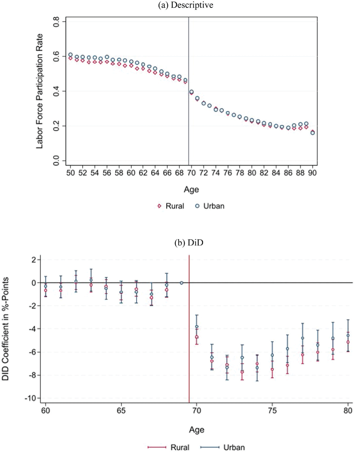
The estimated mortality decline is larger in urban compared to rural areas (Table 5 and Online Appendix event-time Figure E.9).Footnote 40 The larger impact in urban areas is plausible because mortality in cities was typically higher than in rural areas at the time (a fact known as the urban mortality penalty), which was at least partly driven by higher residential crowding (see, for instance, Davenport Reference Davenport2020). Figure 13 shows that the pension reduced crowding in both rural and urban areas; however, the reduction was much more pronounced in urban areas, supporting the finding of a larger mortality decline in urban areas. This is in line with our crowding mechanism, as Poor Law Relief in cities was more often conditional on residing in workhouses, whereas rural parishes imposed such conditions less stringently (Boyer Reference Boyer2019, table 5.11). We find no evidence for differential effects on labor supply (Figure 14).
PENSION AND MORTALITY: NATIONAL DiD-ESTIMATES, URBAN VS. RURAL

Table 5 Long description
A table comparing the estimated mortality decline in urban and rural areas. The table has two columns: Coefficient and Observations. It contains two rows labeled Rural and Urban. Row 1: Rural, Coefficient -0.043 (-1.81), Observations 104. Row 2: Urban, Coefficient -0.078* (-2.21), Observations 104.
* = Significant at the 10 percent level.
** = Significant at the 5 percent level.
Notes: Coefficients from a difference-in-difference model (interaction of post-treatment-period and treatment dummy). Dependent variable: detrended ln(mortality rates). Years 1901–1913. The estimated mortality reduction is larger, compared to the baseline estimates, because of differently constructed population size data (inter- and extrapolation at the district level). Standard errors clustered at the age-group level using wild-bootstrap. t-value in parentheses.
Source: See Table 1.
PENSION AND NUMBER OF RESIDENTS PER HOUSEHOLD, RURAL VS. URBAN
Notes: Panel b): Each dot represents a 2×2 difference-in-difference coefficient (and 95 percent confidence bands) comparing the change in average number of residents per household between 1901 (before) and 1911 (after) for each age (60–80) relative to the reference age 69. Equations are estimated separately for rural and urban areas. The vertical line indicates the age-based eligibility threshold that was introduced by the pension in 1909.
Source: Own calculations based on individual full-count census data for England and Wales provided by IPUMS.

Figure 13 Long description
The image contains two graphs that analyze the number of residents per household in rural and urban areas. Panel A is a scatter plot showing the average number of residents per household against age, with separate data series for rural and urban areas. The x-axis represents age, ranging from 50 to 90 years, and the y-axis represents the average number of residents per household, ranging from 0 to 200. The rural data series is represented by red diamonds, and the urban data series is represented by blue circles. The plot shows that the average number of residents per household increases with age in urban areas, while it remains relatively stable in rural areas. Panel B is a line graph showing the difference-in-difference (DiD) coefficient in percentage points against age, with separate data series for rural and urban areas. The x-axis represents age, ranging from 60 to 80 years, and the y-axis represents the DiD coefficient in percentage points, ranging from -50 to 10. The rural data series is represented by red diamonds, and the urban data series is represented by blue circles. The graph shows that the DiD coefficient for urban areas decreases significantly after the age of 70, while it remains relatively stable for rural areas. The vertical line at age 70 indicates the age-based eligibility threshold introduced by the pension in 1909.
PENSION AND LABOR FORCE PARTICIPATION, URBAN VS. RURAL
Notes: Panel b): Each dot represents a 2×2 difference-in-difference coefficient (and 95 percent confidence bands) comparing the change in the labor force participation rate between 1901 (before) and 1911 (after) for each age (60–80) relative to the reference age 69. Equations are estimated separately for rural and urban areas. The vertical line indicates the age-based eligibility threshold that was introduced by the pension in 1909. Source: Own calculations based on individual full-count census data for England and Wales provided by IPUMS.

Gender
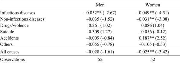
Table 6, showing the mortality DiD estimates separately for men and women, documents that the estimated mortality decline was slightly larger for men, which is also supported by the DiD event-time-estimates (see Online Appendix Figure E.10). Given that male mortality is more volatile than female mortality, standard errors of the estimate, however, are higher for men, rendering the overall coefficient insignificant. The finding of a similarly sized or even slightly larger mortality effect for men is nonetheless surprising, given that pension recipiency rates were higher for women (63 percent of women 70+ received a pension in 1911) than for men (49 percent).Footnote 41
PENSION AND MORTALITY: NATIONAL DiD-ESTIMATES, MEN VS. WOMEN

Table 6 Long description
A table comparing mortality DiD estimates for men and women. The table has 11 rows and 3 columns. The columns are labeled Men, Women, and Observations. The rows are labeled with different causes of mortality: Infectious diseases, Non-infectious diseases, Drugs/violence, Suicide, Accidents, Others, All causes, and Observations. Each row contains values for men and women, including coefficients and standard errors in parentheses. For Infectious diseases, men have a coefficient of -0.052 with a standard error of -2.67, and women have a coefficient of -0.049 with a standard error of -4.51. For Non-infectious diseases, men have a coefficient of -0.035 with a standard error of -1.52, and women have a coefficient of -0.031 with a standard error of -3.08. For Drugs/violence, men have a coefficient of 0.261 with a standard error of 1.02, and women have a coefficient of 0.086 with a standard error of 1.04. For Suicide, men have a coefficient of 0.309 with a standard error of 1.27, and women have a coefficient of -0.056 with a standard error of -0.12. For Accidents, men have a coefficient of -0.009 with a standard error of -0.84, and women have a coefficient of 0.187 with a standard error of 2.52. For Others, men have a coefficient of -0.055 with a standard error of -0.78, and women have a coefficient of -0.105 with a standard error of -0.53. For All causes, men have a coefficient of -0.028 with a standard error of -1.61, and women have a coefficient of -0.025 with a standard error of -3.42. The Observations row shows that there are 52 observations for both men and women.
* = Significant at the 10 percent level.
** = Significant at the 5 percent level.
Notes: Coefficients from a difference-in-difference model (interaction of post-treatment-period and treatment dummy). Dependent variable: detrended ln(mortality rates). Years 1901–1913. Equations are estimated separately for men and women. Standard errors clustered at the age-group level using wild-bootstrap. t-value in parentheses.
Source: See Table 1.
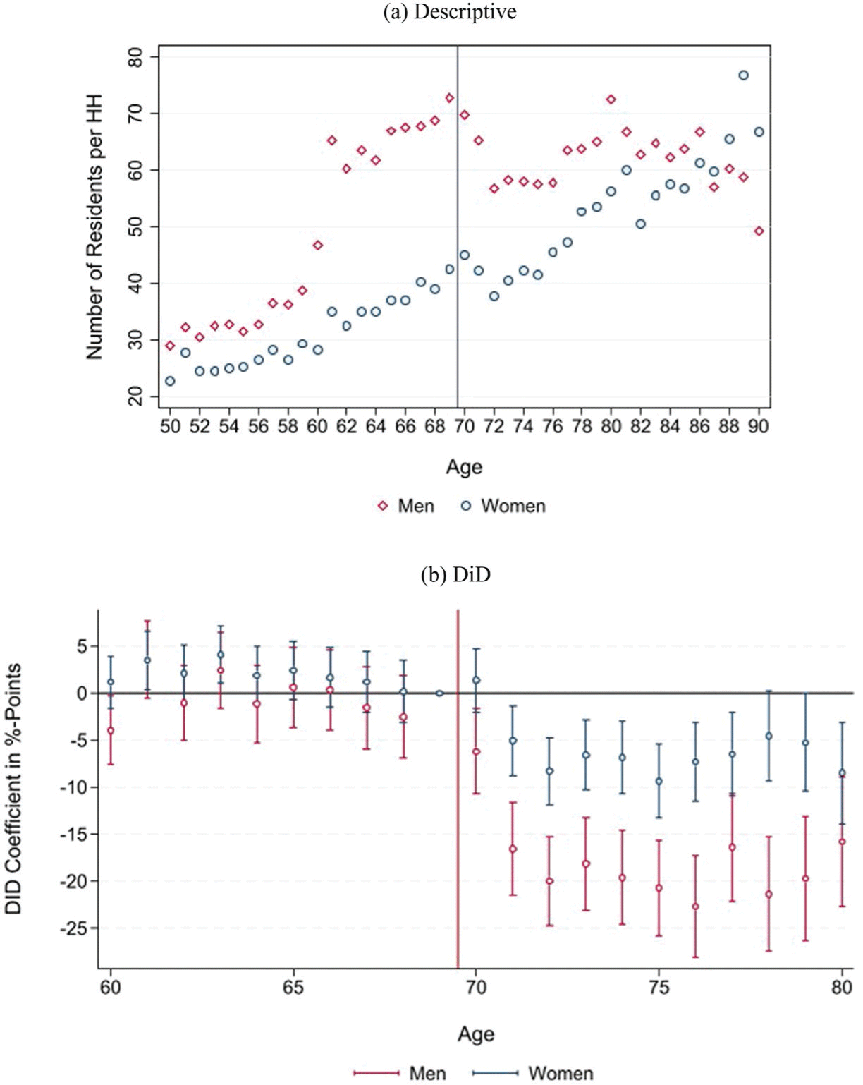
The potential paradox is resolved by the fact that observed behavioral responses were larger for men. Both residential crowding and labor supply fell more for men than for women. Figure 15 documents that the number of residents per household and the share of people living in poorhouses show a stronger reduction for men. This aligns with the fact that prior to the pension, men were significantly more likely than women to be relieved in workhouses (Boyer Reference Boyer2019).Footnote 42 Elderly men were particularly likely to enter workhouses during the winter months, with relief rates 20 to 25 percent higher in January than in July. This seasonal pattern is consistent with the observed decline in male mortality from infectious diseases after the pension (Table 6). Moreover, more men than women retired as a response to the reform (Figure 16), which is historically plausible given that labor earnings were a more important source of income in old age for men than for women before the reform (Boyer Reference Boyer2019, table 5.7), which potentially contributed to lower mortality from non-infectious diseases.
PENSION AND NUMBER OF RESIDENTS PER HOUSEHOLD, MEN VS. WOMEN
Notes: Panel b): Each dot represents a 2×2 difference-in-difference coefficient (and 95 percent confidence bands) comparing the change in average number of residents per household between 1901 (before) and 1911 (after) for each age (60–80) relative to the reference age 69. Equations are estimated separately for men and women. The vertical line indicates the age-based eligibility threshold that was introduced by the pension in 1909.
Source: Own calculations based on individual full-count census data for England and Wales provided by IPUMS.

PENSION AND LABOR FORCE PARTICIPATION, MEN VS. WOMEN
Notes: Panel b): Each dot represents a 2×2 difference-in-difference coefficient (and 95 percent confidence bands) comparing the change in labor force participation rates between 1901 (before) and 1911 (after) for each age (60–80) relative to the reference age 69. Equations are estimated separately for men and women. The vertical line indicates the age-based eligibility threshold that was introduced by the pension in 1909.
Source: Own calculations based on individual full-count census data for England and Wales provided by IPUMS.

DISCUSSION
Our estimates of the mortality decline following the pension range between 2.7 percent (national level DiD), 8 percent (national event-time estimate for 1913), to 12.5 percent (county-level analysis). The estimated decline is sizable given that the overall life expectancy gains for the elderly were modest before WWII. Average elderly (75+) mortality rates in the 1930s were only around 12 percent lower than in the 1890s (calculated using data from the Human Mortality Database (2019)). Thus, our estimates suggest that a substantial share of the elderly mortality decline happening between the beginning of the twentieth century and WWII could be driven by the introduction of public pensions. In addition, in the Online Appendix, we approximate the price paid by the pension to postpone deaths and argue that considering reasonable statistical values of life, the reform was welfare-improving.
Compared to previous studies, our results fall well within the range of estimates from contemporary country cases with similar income levels to those of the early twentieth-century United Kingdom. For instance, Barham and Rowberry (Reference Barham and Rowberry2013) estimate a 4 percent mortality reduction in Mexico, whereas Huang and Zhang (Reference Huang and Zhang2021) find a 12 percent mortality reduction in China. Compared to studies on the United States, the estimated mortality decline of the U.K. pension, however, is relatively small. Balan-Cohen (Reference Balan-Cohen2008) estimates that the expansion of old-age assistance in the United States following the 1935 Social Security Act reduced elderly mortality by more than 20 percent until 1955. More recently, Galofré-Vilà, McKee, and Stuckler (Reference Galofré-Vilà, McKee and Stuckler2022) suggest that the mortality effect was even larger, reducing elderly mortality by almost 40 percent until 1944.Footnote 43 The larger estimated mortality declines for the United States are likely driven by institutional and methodological factors. The reform in the United States took place more than 20 years later, and the retirement age was lower (United Kingdom: 70 vs. United States: 65). Thus, medical technology, health status, and living conditions of the target population in the United States were substantially different.
Methodologically, the results presented in Balan-Cohen (Reference Balan-Cohen2008) and Galofré-Vilà, McKee, and Stuckler (Reference Galofré-Vilà, McKee and Stuckler2022) are based on a substantially longer post-pension period, which we are unable to explore due to the mortality distortions caused by WWI. However, it is highly plausible that the positive health effects of the U.K. pension reform have also accumulated over time. The bottom panel of our Figure 7 shows a clear pattern of mortality reductions becoming stronger over time, which fits with the event-time estimates of Figure 2 from Galofré-Vilà, McKee, and Stuckler (Reference Galofré-Vilà, McKee and Stuckler2022), indicating that the pension effect increased almost linearly over time. From the previous studies, we know that the drivers of this time pattern were frictions in the transition to adequate housing,out of dangerous jobs and a cumulative aspect to improving living conditions, which, in turn, positively affects health outcomes and life expectancy in the long run. Thus, restricting the post-pension period to 4 years, as in our study, would substantially lower the estimated mortality decline for the United States. Applying the U.S. pattern to our setting suggests that our effects might have been twice as high after nine years, which is the time frame analyzed in Galofré-Vilà, McKee, and Stuckler (Reference Galofré-Vilà, McKee and Stuckler2022).
CONCLUSION
In this paper, we have argued that the introduction of old-age assistance in the United Kingdom has postponed an economically relevant number of elderly deaths by reducing residential crowding and allowing elderly people to retire from jobs associated with high occupation-specific mortality rates. Our estimates are consistent with the idea that the introduction of old-age assistance is responsible for a large share of the elderly mortality decline in the United Kingdom between the beginning of the twentieth century and WWII. Thus, as one of the few, this study highlights the potentially large contribution of early social security reforms to the historical mortality decline. Our findings might also be relevant for today’s developing countries that plan to introduce noncontributory (a.k.a. social) pensions. These countries often share some of the characteristics of the United Kingdom in the early twentieth century, such as a lack of a comprehensive welfare system, relatively high mortality rates, crowded living spaces, and, at least in certain sectors, health-detrimental work environments.
 (Deaths(75−84)+Deaths(85+))∗1000Pop(75−84)+Pop(85+)
 (Deaths(45−54)+Deaths(55−64))∗1000Pop(45−54)+Pop(55−64)




 Open access

