1 Introduction
In numerous applications, turbulent boundary layers (TBLs) are exposed to, and interact with, free-stream vortical perturbations. For example, in industrial flows such as those of turbomachinery and heat exchangers, the incoming stream can include free-stream perturbations that buffet the TBL developing on the wall. The present work examines this interaction using direct numerical simulations. A zero-pressure-gradient (ZPG) TBL is simulated beneath quiescent and vortical free streams, and the two conditions are contrasted.
Earlier studies have experimentally investigated the effect of grid-generated free-stream turbulence (FST) with intensities mostly less than
 $7\,\%$
(Simonich & Bradshaw Reference Simonich and Bradshaw1978; Hancock & Bradshaw Reference Hancock and Bradshaw1983, Reference Hancock and Bradshaw1989; Castro Reference Castro1984). These studies showed that FST mainly influences the wake region of the mean-velocity profile. The FST depresses the wake region, or reduces
 $U_{\infty }/u_{\unicode[STIX]{x1D70F}}$
, where
 $U_{\infty }$
and
 $u_{\unicode[STIX]{x1D70F}}$
are the free-stream and friction velocities, respectively. Simonich & Bradshaw (Reference Simonich and Bradshaw1978) reported that the increases in skin friction and heat transfer are nearly proportional to the turbulent intensity only. In their study, skin friction and heat transfer increased by 2 % and 5 %, respectively, for 1 % increase in the FST intensity. Hancock & Bradshaw (Reference Hancock and Bradshaw1983) tried to capture the effects of FST with a single parameter
 $\unicode[STIX]{x1D6FD}=(Tu/U_{\infty })/((L_{u}/\unicode[STIX]{x1D6FF})+2)$
, where
 $Tu$
,
 $L_{u}$
and
 $\unicode[STIX]{x1D6FF}$
are the turbulence intensity and dissipation length scale and the boundary-layer thickness; the mean skin friction was shown to increase with the parameter
 $\unicode[STIX]{x1D6FD}$
. Blair (Reference Blair1983) and Castro (Reference Castro1984) suggested a modification to the parameter in order to take account of the low-Reynolds-number effect (
 $Re_{\unicode[STIX]{x1D703}}<2000$
) whereby the FST becomes less effective at increasing drag.
Hancock & Bradshaw (Reference Hancock and Bradshaw1989) performed conditional sampling to investigate the contribution of FST to flow statistics. In their study, the boundary-layer fluid was thermally identified by heating the plate. They reported the conditional contributions of the free-stream and boundary-layer fluids to the Reynolds-stress profiles and triple products. In their study, the conditional perturbation statistics were evaluated relative to the conventional time average (or unconditional) mean. They showed that shear-stress correlation coefficient (
 $-\overline{u^{\prime }v^{\prime }}/u_{rms}^{\prime }v_{rms}^{\prime }$
) is reduced because the isotropic FST effectively destroys the coherence of the perturbations inside the boundary layer.
Further studies were performed with high turbulence intensities, greater than
 $10\,\%$
, generated by gas turbine combustors (Ames & Moffat Reference Ames and Moffat1990) or high-velocity cross jets (Thole & Bogard Reference Thole and Bogard1995, Reference Thole and Bogard1996). Ames & Moffat (Reference Ames and Moffat1990) proposed a new parameter which considers the momentum-thickness Reynolds number,
 $Re_{\unicode[STIX]{x1D703}}$
, in addition to
 $L_{u}$
and
 $Tu$
for predicting skin-friction enhancement. But Thole & Bogard (Reference Thole and Bogard1995) demonstrated that the increase in skin friction with the Hancock parameter,
 $\unicode[STIX]{x1D6FD}$
, is sufficiently accurate up to
 $Tu=28\,\%$
. Thole & Bogard (Reference Thole and Bogard1996) found that even the highest levels of FST considered mostly influence the outer region of the boundary layer, and have negligible effects on the logarithmic region. However, they provided evidence that the strong FST penetrates into the boundary layer very close to the wall, by performing hot-wire measurements of the streamwise velocity fluctuations: the energy spectrum of the near-wall region was similar to that of the FST. While the above studies examined the influence of FST on TBLs experimentally, Péneau, Boisson & Djilali (Reference Péneau, Boisson and Djilali2000) performed large-eddy simulations to examine the effect of strong FST up to
 $Tu=21\,\%$
. They used random Oseen vortices for generating inflow FST, which was therefore neither homogeneous nor isotropic. They reported that the increase in skin friction is almost unchanged irrespective of the FST intensity for
 $7\,\%<Tu<21\,\%$
, but their domain size was too short (
 $Re_{\unicode[STIX]{x1D703}}\approx 1200$
–
 $1500$
) to observe the interactions between FST and TBL at higher Reynolds number.
The influence of the FST length scale on the changes within the boundary layer can be gleaned by contrasting results from different studies. Sharp, Neuscamman & Warhaft (Reference Sharp, Neuscamman and Warhaft2009) examined the effect of large-scale FST, and showed that the Reynolds stresses normalized by the friction velocity increase relative to their values in canonical boundary layers. They also reported the emergence of an outer peak in the pre-multiplied energy spectra when the boundary layer is subjected to FST. Such a peak is known to occur in unforced boundary layers, although at appreciably higher Reynolds numbers (Hutchins & Marusic Reference Hutchins and Marusic2007), and is associated with large-scale motions that reach many boundary-layer thicknesses in streamwise extent and modulate the near-wall structures (Mathis, Hutchins & Marusic Reference Mathis, Hutchins and Marusic2009; Hwang et al.
Reference Hwang, Lee, Sung and Zaki2016). In contrast to the work by Sharp et al. (Reference Sharp, Neuscamman and Warhaft2009), Nagata, Sakai & Komori (Reference Nagata, Sakai and Komori2011) considered small-scale FST (
 $L_{u}/\unicode[STIX]{x1D6FF}\ll 1$
) with relatively low turbulent intensity
 $(Tu<2.4\,\%)$
. They demonstrated that the skin friction still increases, even though the rate of production of turbulence kinetic energy is reduced along with the Reynolds normal and shear stresses, normalized by the friction velocity. In addition, the outer peak in the pre-multiplied energy spectra was not observed in the experiments by Nagata et al. (Reference Nagata, Sakai and Komori2011). These results are unique since most other efforts have focused on larger FST length scales.
The outer peak in the energy spectra was also reported by Li, Schlatter & Henningson (Reference Li, Schlatter and Henningson2010) who performed large-eddy simulations of boundary layers beneath FST at Reynolds numbers in the range
 $Re_{\unicode[STIX]{x1D703}}\approx 100$
–
 $1000$
. Their result is curious because their boundary layer was initially transitional and had not reached an equilibrium state. Recently, Dogan, Hanson & Ganapathisubramani (Reference Dogan, Hanson and Ganapathisubramani2016) experimentally evaluated the effect of large-scale FST on the near-wall region. They reported an increase in the near-wall streamwise velocity fluctuations with FST intensity. Using a scale decomposition, they separated the small- and large-scale contributions, and attributed the increase to the latter. Dogan, Hearst & Ganapathisubramani (Reference Dogan, Hearst and Ganapathisubramani2017) showed a close correlation between the large-scale velocity signals in the buffer and logarithmic layers by performing multipoint measurements. Subsequently, Hearst, Dogan & Ganapathisubramani (Reference Hearst, Dogan and Ganapathisubramani2018) identified within the spectrogram zones that are affected by the free-stream spectrum and a universal small-scale inner peak. Since the latter was unchanged by the forcing, they concluded that only the large-scale components of the FST penetrate down to the near-wall region.
Previous experiments and simulations have quantified the increase in drag when boundary layers are exposed to free-stream forcing, and how this effect depends on the intensity and length scale of FST. The exact mechanism that leads to the increase in skin friction is, however, less clear. The objective of the current study is to investigate how the free-stream fluid statistically and dynamically causes this increase. Therefore, an important consideration is to objectively distinguish the free-stream fluid and its contribution to flow statistics – a requirement that is difficult to achieve experimentally and that has not been performed numerically to date. We adopted a method similar to that of the work by Hancock & Bradshaw (Reference Hancock and Bradshaw1989). They heated the boundary-layer fluid, although the finite Prandtl number,
 $Pr$
, in the experiments reduces the accuracy of separating the two streams. In our simulations, we have the advantage that we employ a level-set approach which represents an infinite
 $Pr$
and thus maintains a sharp virtual interface between the boundary-layer and free-stream fluids. Using conditional sampling, we examine how the FST modifies the boundary-layer statistics and flow structures, and leads to drag increase.
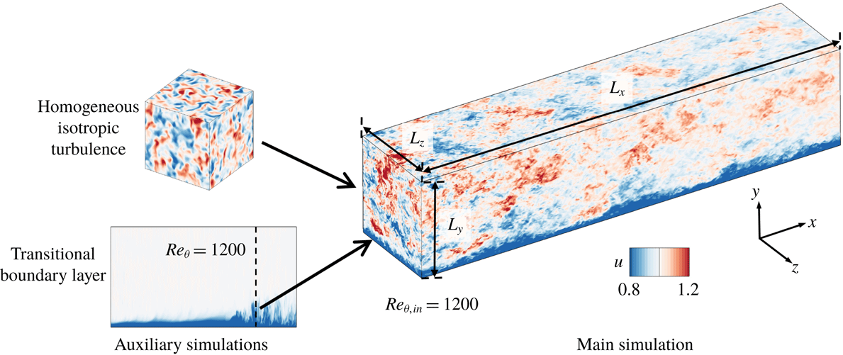
A schematic diagram of the computational set-up is shown in figure 1. Two main simulations are performed, the first of a canonical TBL and the second additionally includes homogeneous isotropic turbulence (HIT) with
 $10\,\%$
intensity in the free stream. Comparing the downstream evolutions of the two flows highlights the impact of the newly introduced free-stream forcing on the boundary layer. The configuration thus differs from experiments where both the boundary layer and free-stream turbulence evolve together from the leading edge. Our domain length ensures that the momentum-thickness Reynolds number of the forced boundary layer exceeds
 $Re_{\unicode[STIX]{x1D703}}=3200$
before the exit plane, which is higher than the Reynolds numbers in previous numerical studies.
The paper is organized into six sections. A description of the numerical method and the inflow condition is provided in § 2. Section 3 includes the conditional sampling approach, and a quantitative comparison of conditional statistics based on the level set and the vorticity magnitude for a conventional boundary layer. Section 4 demonstrates the influence of FST on the skin friction and reports the conditional statistics of the forced flow. Section 5 discusses the effect of FST on the turbulent flow structures, and conclusions are summarized in the last section.
Schematic of the flow configuration showing the precursor transitional boundary layer and HIT, and the fully turbulent flow downstream.

2 Simulation details
The continuity and Navier–Stokes equations for incompressible flow are
 $$\begin{eqnarray}\displaystyle & \displaystyle \frac{\unicode[STIX]{x2202}u_{j}}{\unicode[STIX]{x2202}x_{j}}=0, & \displaystyle\end{eqnarray}$$
 $$\begin{eqnarray}\displaystyle & \displaystyle \frac{\unicode[STIX]{x2202}u_{i}}{\unicode[STIX]{x2202}t}+\frac{\unicode[STIX]{x2202}u_{i}u_{j}}{\unicode[STIX]{x2202}x_{j}}=-\frac{\unicode[STIX]{x2202}p}{\unicode[STIX]{x2202}x_{i}}+\frac{1}{Re_{\unicode[STIX]{x1D703}_{in}}}\frac{\unicode[STIX]{x2202}^{2}u_{i}}{\unicode[STIX]{x2202}x_{j}^{2}}. & \displaystyle\end{eqnarray}$$
Terms in the above equations are non-dimensionalized using the free-stream velocity
 $U_{\infty }$
and the momentum thickness at the inlet
 $\unicode[STIX]{x1D703}_{in}$
of the main simulation domain. The momentum-thickness Reynolds number in (2.2) is defined as
 $Re_{\unicode[STIX]{x1D703}_{in}}\equiv \unicode[STIX]{x1D70C}U_{\infty }\unicode[STIX]{x1D703}_{in}/\unicode[STIX]{x1D707}=1200$
. The velocity components in the streamwise (
 $x$
), wall-normal (
 $y$
) and spanwise (
 $z$
) directions are
 $u$
,
 $v$
and
 $w$
, respectively, and the pressure is
 $p$
. Hereafter, a bar denotes a spanwise and time average, and a prime indicates fluctuating quantities according to the Reynolds decomposition, for example
 $u=\overline{u}+u^{\prime }$
.
The flow equations were solved using a fractional step algorithm on a staggered grid with a local volume-flux formulation (Rosenfeld, Kwak & Vinokur Reference Rosenfeld, Kwak and Vinokur1991). The viscous terms were integrated in time implicitly using the Crank–Nicolson method, and the convective terms were treated explicitly using the Adams–Bashforth scheme. The pressure equation is solved by performing Fourier transform in the span, cosine transform in the streamwise direction and a tridiagonal direct solve in the wall-normal coordinate. The algorithm has been used extensively in previous studies of transitional (Nolan & Zaki Reference Nolan and Zaki2013) and fully turbulent wall-bounded flows (Jelly, Jung & Zaki Reference Jelly, Jung and Zaki2014; Lee, Sung & Zaki Reference Lee, Sung and Zaki2017).
Validation of inflow TBL. (a) Mean streamwise velocity and (b) root-mean-square fluctuations in inner scaling; (——) inflow TBL in main simulation and (○) data by Schlatter & Örlü (Reference Schlatter and Örlü2010) at
 $Re_{\unicode[STIX]{x1D703}}=1410$
.

2.1 Computational set-up
A schematic of the flow configuration is shown in figure 1. In order to generate a realistic inflow TBL for the main computations, a precursor simulation of a transitional boundary layer was performed. A spatially and temporally resolved cross-flow plane was stored in the fully turbulent regime and used as inflow in the main simulation. A similar approach was adopted by Lee et al. (Reference Lee, Jung, Sung and Zaki2013) and Lee et al. (Reference Lee, Sung and Zaki2017). The inflow condition in the auxiliary transitional computation is a Blasius boundary layer and a superposition of vortical perturbations which were prescribed inside the mean shear only, such that the transitional boundary layer develops below a quiescent free stream (in contrast to bypass transition). The domain length spanned
 $108\leqslant Re_{\unicode[STIX]{x1D703}}\leqslant 1379$
which overlaps with the main simulation domain. Instantaneous TBL data were extracted in the precursor simulation at
 $Re_{\unicode[STIX]{x1D703}}=1200$
. The time series was subsequently applied at the inlet in the main simulation. Even though the inflow Reynolds number is lower than the recommendation by Schlatter & Örlü (Reference Schlatter and Örlü2012), the streamwise extent of the domain ensures that their criterion is satisfied where results are examined. In addition, the accuracy of this inflow condition was extensively validated. Figure 2 compares the mean streamwise velocity profile
 $\overline{u}$
and the root-mean-square fluctuations
 $u_{i,rms}^{\prime }$
in inner scaling with the data from Schlatter & Örlü (Reference Schlatter and Örlü2010). The profiles are scaled by the friction velocity
 $u_{\unicode[STIX]{x1D70F}}\equiv \sqrt{\unicode[STIX]{x1D708}(\unicode[STIX]{x2202}\overline{u}/\unicode[STIX]{x2202}y)|_{y=0}}$
, where
 $\unicode[STIX]{x1D708}$
is the kinematic viscosity and
 $y^{+}\equiv (yu_{\unicode[STIX]{x1D70F}})/\unicode[STIX]{x1D708}$
.
In addition to the inflow boundary layer, free-stream vortical perturbations are needed at the inlet. Decaying, HIT was simulated in a rectangular box with dimensions
 $\{L_{x},L_{y},{L_{z}\}}_{HIT}=$
 $\{80,80,160\}\,\unicode[STIX]{x1D703}_{in}$
using a pseudo-spectral algorithm, with periodic boundary conditions in all three coordinate directions. Both
 $x$
and
 $y$
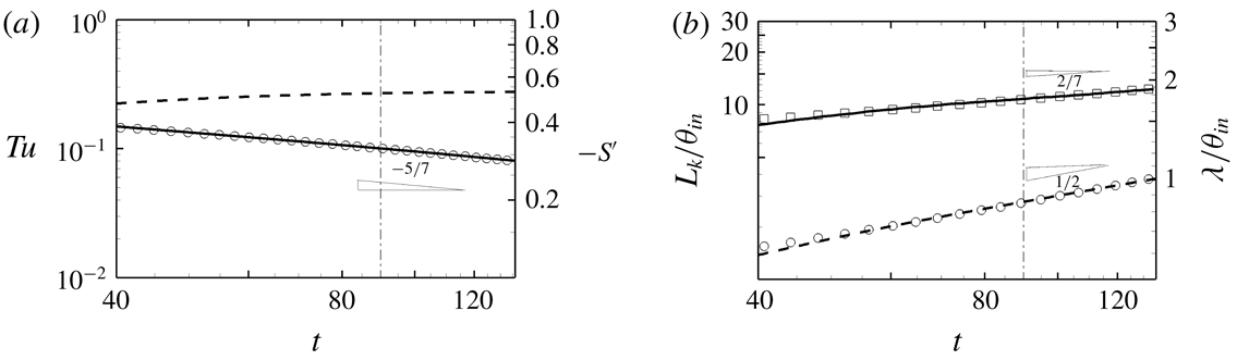
were discretized using 640 Fourier modes, and 1280 modes were used in the spanwise direction. Figure 3 shows the time history of the turbulent intensity, skewness of the velocity derivative, integral length scale and Taylor microscale:
 $$\begin{eqnarray}Tu\equiv \sqrt{\frac{u^{\prime 2}+v^{\prime 2}+w^{\prime 2}}{3}},\quad S^{\prime }(u^{\prime })\equiv \frac{\overline{(\unicode[STIX]{x2202}u^{\prime }/\unicode[STIX]{x2202}t)^{3}}}{(\overline{(\unicode[STIX]{x2202}u^{\prime }/\unicode[STIX]{x2202}t)^{2}})^{3/2}},\quad L_{k}\equiv \frac{k^{3/2}}{\unicode[STIX]{x1D716}},\quad \unicode[STIX]{x1D706}\equiv \sqrt{\frac{15\unicode[STIX]{x1D708}\overline{u^{\prime 2}}}{\unicode[STIX]{x1D716}}}.\end{eqnarray}$$
In the above expressions,
 $k$
is the turbulence kinetic energy and
 $\unicode[STIX]{x1D716}$
is the dissipation rate. The time instant when the data are extracted is identified by a dashed-dotted line in the figure (
 $Tu=0.1$
and
 $L_{k}\approx 10.8\unicode[STIX]{x1D703}_{in}$
). Note that
 $S^{\prime }$
is approaching its asymptotic value (Batchelor Reference Batchelor1953). At the time when the data are extracted, the Reynolds number based on the Taylor microscale is
 $Re_{\unicode[STIX]{x1D706}}$
 $\equiv u_{rms}^{\prime }\unicode[STIX]{x1D706}/\unicode[STIX]{x1D708}=105$
. The turbulence intensity follows the decay law
 $Tu\propto t^{-5/7}$
, and the length scale shows a consistent power-law dependence
 $L_{k}\propto t^{2/7}$
.
The three-dimensional energy spectrum for the inflow FST is provided in figure 4(a). The height of the plateau in
 $E(\unicode[STIX]{x1D705}\unicode[STIX]{x1D702})$
, or the Kolmogorov constant
 $C_{k}$
, is approximately 1.96. The spatial resolution of a spectral simulation is adequate since
 $\unicode[STIX]{x1D705}_{max}\unicode[STIX]{x1D702}>1$
, where
 $\unicode[STIX]{x1D705}_{max}$
is the maximum wavenumber and
 $\unicode[STIX]{x1D702}$
is the Kolmogorov scale.
The free-stream disturbances at the inflow of the main simulations are extracted from the HIT data using Taylor’s hypothesis, where space is converted to time using the free-stream velocity of the boundary layer,
 $(U_{\infty },V_{\infty })$
at
 $Re_{\unicode[STIX]{x1D703},in}=1200$
. Note that periodicity of the free-stream forcing is not a concern because the underlying TBL is time dependent and not periodic. We have also exploited isotropy of the free stream and rotated the HIT volume about its
 $z$
-axis by
 $\unicode[STIX]{x1D709}=7.829^{\circ }$
. In this manner, every
 $L_{x,HIT}/(U_{\infty }\cos \unicode[STIX]{x1D709})$
time units, the HIT plane prescribed as inflow to the direct numerical simulation is shifted vertically by
 $L_{x,HIT}\tan (\unicode[STIX]{x1D709})=11\unicode[STIX]{x1D703}_{in}$
, which is of the same order as the integral length scale.
Evolution of HIT in time. The dashed-dotted line marks the time instant when data are extracted to apply as inflow condition in the main simulation. (a) (——)
 $Tu$
, (○)
 $Tu\propto t^{-5/7}$
and (– – –)
 $-S^{\prime }$
; (b) (——)
 $L_{k}$
, (▫)
 $L_{k}\propto t^{2/7}$
, (– – –)
 $\unicode[STIX]{x1D706}$
and (○)
 $\unicode[STIX]{x1D706}\propto t^{0.5}$
.

(a) Three-dimensional energy spectrum of the FST at the inlet. (b) Comparison of downstream evolution of FST in the main simulation: (——)
 $u_{rms}^{\prime }$
, (– – –)
 $v_{rms}^{\prime }$
, (— ⋅ —)
 $w_{rms}^{\prime }$
and (○)
 $Tu$
of the decaying turbulence (reproduced from figure 3
a). (c) Downstream evolution of the integral length scale,
 $L_{k}/\unicode[STIX]{x1D6FF}_{99}$
. Thin dashed-dotted lines mark streamwise positions where
 $Re_{\unicode[STIX]{x1D703}}=\{1900,3000\}$
in FRC computation.

The dimensions of the computational domains, the number of grid points and resolutions are provided in table 1. Two simulations are contrasted: one of a conventional TBL beneath a quiescent free stream and a second case with free-stream vortical forcing. They are designated the reference (REF) and forced (FRC) cases (an additional forced case with smaller-scale HIT is reported in appendix B). In the forced configuration, the FST decays with downstream distance, and figure 4(b,c) shows the evolution of its normal stresses and length scale. The Reynolds normal stresses are isotropic, and their decay in space in the main simulation matches the temporal evolution of
 $Tu$
shown in figure 3(a), and reproduced in figure 4(b) (circle symbols). The length scale of FST is now redefined as
 $L_{k}\equiv -k^{3/2}/U_{\infty }(\text{d}k/\text{d}x)$
, and remains of the order of the
 $99\,\%$
boundary-layer thickness,
 $\unicode[STIX]{x1D6FF}_{99}$
(figure 4
c). This choice is motivated by our understanding of the interaction of vortical perturbations with mean shear: disturbances with spanwise and wall-normal length scales of the order of the boundary-layer thickness, and elongated in the streamwise direction, are most effective at permeating the mean shear and inducing an energetic response (Zaki & Durbin Reference Zaki and Durbin2005; Zaki & Saha Reference Zaki and Saha2009). For the present FST, the first two criteria are satisfied and the low-frequency components of the streamwise wavenumbers satisfy the third one.
Summary of simulation parameters, and the spatial and temporal resolutions.

Both the REF and FRC boundary-layer simulations start at the same streamwise position,
 $Re_{\unicode[STIX]{x1D703},in}=1200$
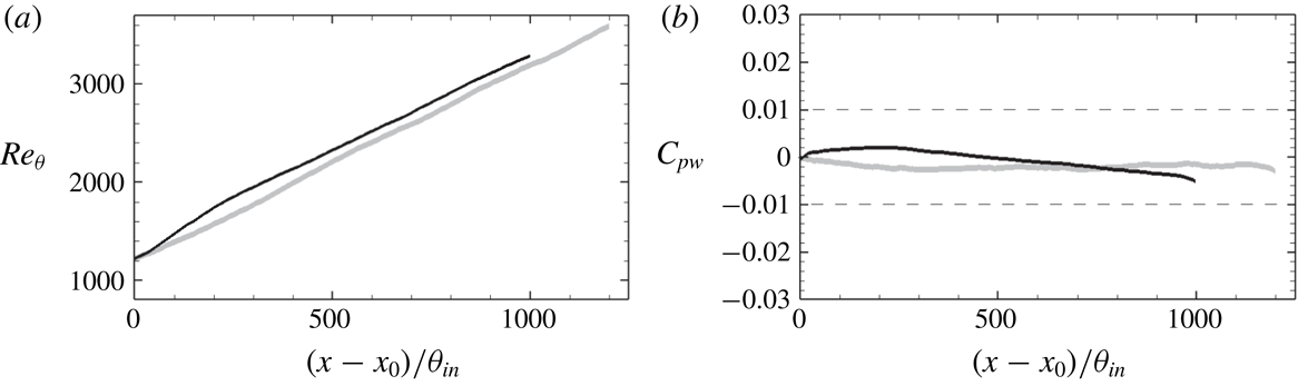
. The differences in lengths and widths of the domains were guided by results from preliminary simulations. The domain of the FRC case is slightly shorter in the streamwise direction, which is partially compensated by a faster increase in the momentum-thickness Reynolds number (see figure 5). Its larger spanwise extent is required to accommodate the formation of wider structures. In both cases, the grid is uniformly spaced in the streamwise and spanwise directions, whereas a non-uniform grid distribution is used in the wall-normal direction. The grid spacings reported in table 1 in wall units are normalized by the friction velocity at the inlet to the simulation domain.
Downstream dependence of (a) momentum-thickness Reynolds number
 $Re_{\unicode[STIX]{x1D703}}\equiv U_{\infty }\unicode[STIX]{x1D703}/\unicode[STIX]{x1D708}$
and (b) mean pressure coefficient at the wall
 $C_{pw}$
. Grey: reference simulation; black: forced case.

The convective outflow condition
 $\unicode[STIX]{x2202}u_{i}/\unicode[STIX]{x2202}t+c\unicode[STIX]{x2202}u_{i}/\unicode[STIX]{x2202}x=0$
is applied at the outlet of the simulation domain, where
 $c$
is the local bulk velocity. The no-slip condition is imposed at the bottom wall. Periodic boundary conditions are applied in the spanwise direction. At the top boundary, appropriate treatment is required to maintain a ZPG boundary layer, even in the presence of high levels of FST.
2.2 Top boundary condition
A distribution of suction velocity is applied at the top boundary in order to maintain ZPG in the streamwise direction. The suction velocity is evaluated using an active controller. First, a measure of the streamwise free-stream velocity is evaluated and used as a sensor:
 $$\begin{eqnarray}\displaystyle u_{s}(x;t)=\frac{1}{\unicode[STIX]{x1D70F}}\int _{t-\unicode[STIX]{x1D70F}}^{t}\frac{\displaystyle \int _{0}^{L_{y}}\int _{0}^{L_{z}}(1-\unicode[STIX]{x1D6E4}(\boldsymbol{x},t))u(\boldsymbol{x},t)\,\text{d}z\,\text{d}y}{\displaystyle \int _{0}^{L_{y}}\int _{0}^{L_{z}}(1-\unicode[STIX]{x1D6E4}(\boldsymbol{x},t))\,\text{d}z\,\text{d}y}\,\text{d}t, & & \displaystyle\end{eqnarray}$$
where
 $\unicode[STIX]{x1D70F}$
is an averaging time scale for the controller and
 $\unicode[STIX]{x1D6E4}$
is an indicator function which is zero in the free stream and unity in the boundary layer. The method for defining
 $\unicode[STIX]{x1D6E4}$
is covered in the next section. The averaged streamwise velocity
 $u_{\unicode[STIX]{x1D70F}}$
during
 $\unicode[STIX]{x1D70F}$
is
 $$\begin{eqnarray}\displaystyle u_{\unicode[STIX]{x1D70F}}(x,y;t)=\frac{1}{\unicode[STIX]{x1D70F}}\frac{1}{L_{z}}\int _{t-\unicode[STIX]{x1D70F}}^{t}\int _{0}^{L_{z}}u(\boldsymbol{x},t)\,\text{d}z\,\text{d}t. & & \displaystyle\end{eqnarray}$$
The suction velocity at the top boundary is computed as a superposition of continuity constraint over time
 $\unicode[STIX]{x1D70F}$
and the action of the controller:
 $$\begin{eqnarray}\displaystyle v_{top}(x;t)=-\frac{\text{d}}{\text{d}x}\int _{0}^{L_{y}}u_{\unicode[STIX]{x1D70F}}(x,y;t)\,\text{d}y+\unicode[STIX]{x1D70E}\frac{V_{\infty }}{U_{\infty }}(u_{s}(x;t)-u_{T}(x)), & & \displaystyle\end{eqnarray}$$
where
 $u_{T}$
is the target streamwise free-stream velocity which is unity in ZPG. The control factor is
 $\unicode[STIX]{x1D70E}$
, and
 $V_{\infty }/U_{\infty }$
is a reference rate of free-stream vertical to streamwise velocities for the canonical mean boundary-layer profile. The boundary conditions on the other directions are
 $u_{top}=1$
and
 $(\unicode[STIX]{x2202}w/\unicode[STIX]{x2202}y)_{top}=0$
. In the present study, the time scale
 $\unicode[STIX]{x1D70F}$
is comparable to the integral time scale of FST,
 $t_{k}=L_{k}/U_{\infty }$
.
The downstream dependence of pressure coefficient at the wall,
 $$\begin{eqnarray}C_{pw}\equiv \frac{\overline{p}_{(x,y=0)}-\overline{p}_{(x_{0},y=0)}}{\frac{1}{2}\unicode[STIX]{x1D70C}U_{\infty }^{2}},\end{eqnarray}$$
is shown in figure 5. It remains well within the range
 $-0.005<C_{pw}<0.002$
, which satisfies the condition for ZPG.
2.3 Conditional sampling
The starting point for conditional sampling is to define an indicator function,
 $\unicode[STIX]{x1D6E4}(\boldsymbol{x},t)$
, which is unity in the boundary layer and zero in the free stream. Its spanwise and time average is the intermittency,
 $$\begin{eqnarray}\displaystyle \unicode[STIX]{x1D6FE}=\frac{1}{L_{z}\unicode[STIX]{x0394}T}\int _{T_{0}}^{T_{0}+\unicode[STIX]{x0394}T}\int _{0}^{L_{z}}\unicode[STIX]{x1D6E4}(\boldsymbol{x},t)\,\text{d}z\,\text{d}t, & & \displaystyle\end{eqnarray}$$
which is the probability that the fluid is part of the boundary-layer flow. A general quantity
 $\unicode[STIX]{x1D719}$
can then be separated into its boundary-layer
 $\unicode[STIX]{x1D719}^{B}$
and free-stream
 $\unicode[STIX]{x1D719}^{F}$
constituents:
 $$\begin{eqnarray}\displaystyle & \displaystyle \unicode[STIX]{x1D719}^{B}=\unicode[STIX]{x1D6E4}(\boldsymbol{x},t)\unicode[STIX]{x1D719}(\boldsymbol{x},t), & \displaystyle\end{eqnarray}$$
 $$\begin{eqnarray}\displaystyle & \displaystyle \unicode[STIX]{x1D719}^{F}=(1-\unicode[STIX]{x1D6E4}(\boldsymbol{x},t))\unicode[STIX]{x1D719}(\boldsymbol{x},t). & \displaystyle\end{eqnarray}$$
Using this decomposition, the conventional and conditional means are
 $$\begin{eqnarray}\displaystyle & \displaystyle \overline{\unicode[STIX]{x1D719}}=\frac{1}{L_{z}\unicode[STIX]{x0394}T}\int _{T_{0}}^{T_{0}+\unicode[STIX]{x0394}T}\int _{0}^{L_{z}}\unicode[STIX]{x1D719}(\boldsymbol{x},t)\,\text{d}z\,\text{d}t, & \displaystyle\end{eqnarray}$$
 $$\begin{eqnarray}\displaystyle & \displaystyle \overline{\unicode[STIX]{x1D719}}^{B}=\frac{\displaystyle \int _{T_{0}}^{T_{0}+\unicode[STIX]{x0394}T}\int _{0}^{L_{z}}\unicode[STIX]{x1D719}(\boldsymbol{x},t)\unicode[STIX]{x1D6E4}(\boldsymbol{x},t)\,\text{d}z\,\text{d}t}{\displaystyle \int _{T_{0}}^{T_{0}+\unicode[STIX]{x0394}T}\int _{0}^{L_{z}}\unicode[STIX]{x1D6E4}(\boldsymbol{x},t)\,\text{d}z\,\text{d}t}, & \displaystyle\end{eqnarray}$$
 $$\begin{eqnarray}\displaystyle & \displaystyle \overline{\unicode[STIX]{x1D719}}^{F}=\frac{\displaystyle \int _{T_{0}}^{T_{0}+\unicode[STIX]{x0394}T}\int _{0}^{L_{z}}\unicode[STIX]{x1D719}(\boldsymbol{x},t)(1-\unicode[STIX]{x1D6E4}(\boldsymbol{x},t))\,\text{d}z\,\text{d}t}{\displaystyle \int _{T_{0}}^{T_{0}+\unicode[STIX]{x0394}T}\int _{0}^{L_{z}}(1-\unicode[STIX]{x1D6E4}(\boldsymbol{x},t))\,\text{d}z\,\text{d}t}, & \displaystyle\end{eqnarray}$$
where superscripts
 $B$
and
 $F$
identify boundary-layer and free-stream quantities. The conventional mean can be related to boundary-layer and free-stream components, weighted by the local intermittency factor,
 $$\begin{eqnarray}\displaystyle \overline{\unicode[STIX]{x1D719}}=\unicode[STIX]{x1D6FE}\overline{\unicode[STIX]{x1D719}}^{B}+(1-\unicode[STIX]{x1D6FE})\overline{\unicode[STIX]{x1D719}}^{F}. & & \displaystyle\end{eqnarray}$$
Reynolds decomposition can be performed relative to each of the three averages:
 $$\begin{eqnarray}\displaystyle & \displaystyle \unicode[STIX]{x1D719}=\overline{\unicode[STIX]{x1D719}}+\unicode[STIX]{x1D719}^{\prime }, & \displaystyle\end{eqnarray}$$
 $$\begin{eqnarray}\displaystyle & \displaystyle \unicode[STIX]{x1D719}^{B}=\overline{\unicode[STIX]{x1D719}}^{B}+\unicode[STIX]{x1D719}^{\ast }\quad \text{for boundary-layer flow,} & \displaystyle\end{eqnarray}$$
 $$\begin{eqnarray}\displaystyle & \displaystyle \unicode[STIX]{x1D719}^{F}=\overline{\unicode[STIX]{x1D719}}^{F}+\unicode[STIX]{x1D719}^{\prime \prime }\quad \text{for free-stream flow.} & \displaystyle\end{eqnarray}$$
Analysis of the perturbations relative to the conditional means is intended to examine the turbulence dynamics within each region of the flow, separately. In contrast, Hancock & Bradshaw (Reference Hancock and Bradshaw1989) evaluated conditional statistics of perturbation quantities relative to the conventional mean, in order to measure the contribution from each fluid to overall statistics.
Unlike the intermittency weighted average (2.14), higher-order statistics evaluated relative to conditional and conventional means are related by more elaborate expressions. For example, the Reynolds stress is given by
 $$\begin{eqnarray}\overline{u_{i}^{\prime }u_{j}^{\prime }}=\unicode[STIX]{x1D6FE}\overline{u_{i}^{\ast }u_{j}^{\ast }}^{B}+(1-\unicode[STIX]{x1D6FE})\overline{u_{i}^{\prime \prime }u_{j}^{\prime \prime }}^{F}+\unicode[STIX]{x1D6FE}(1-\unicode[STIX]{x1D6FE})(\overline{u_{i}}^{F}-\overline{u_{i}}^{B})(\overline{u_{j}}^{F}-\overline{u_{j}}^{B}).\end{eqnarray}$$
Also, commutation of conditional averaging and the derivative operator is not always possible, for example,
 $$\begin{eqnarray}\displaystyle \overline{\frac{\unicode[STIX]{x2202}\overline{\unicode[STIX]{x1D719}}^{B}}{\unicode[STIX]{x2202}x_{i}}}^{B}=\frac{\unicode[STIX]{x2202}\overline{\unicode[STIX]{x1D719}}^{B}}{\unicode[STIX]{x2202}x_{i}};\quad \overline{\frac{\unicode[STIX]{x2202}\unicode[STIX]{x1D719}}{\unicode[STIX]{x2202}x_{i}}}^{B}=\frac{\unicode[STIX]{x2202}\overline{\unicode[STIX]{x1D719}}^{B}}{\unicode[STIX]{x2202}x_{i}}+\overline{\frac{\unicode[STIX]{x2202}\unicode[STIX]{x1D719}^{\ast }}{\unicode[STIX]{x2202}x_{i}}}^{B}\neq \frac{\unicode[STIX]{x2202}\overline{\unicode[STIX]{x1D719}}^{B}}{\unicode[STIX]{x2202}x_{i}}, & & \displaystyle\end{eqnarray}$$
and similarly for
 $F$
. This affects various terms in the turbulence kinetic energy budget (see appendix A), for example the pseudo-dissipation:
 $$\begin{eqnarray}\displaystyle \frac{1}{Re}\overline{\frac{\unicode[STIX]{x2202}u_{i}^{\prime }}{\unicode[STIX]{x2202}x_{k}}\frac{\unicode[STIX]{x2202}u_{i}^{\prime }}{\unicode[STIX]{x2202}x_{k}}} & = & \displaystyle \frac{1}{Re}\left\{\unicode[STIX]{x1D6FE}\overline{\frac{\unicode[STIX]{x2202}u_{i}^{\ast }}{\unicode[STIX]{x2202}x_{k}}\frac{\unicode[STIX]{x2202}u_{i}^{\ast }}{\unicode[STIX]{x2202}x_{k}}}^{B}+(1-\unicode[STIX]{x1D6FE})\overline{\frac{\unicode[STIX]{x2202}u_{i}^{\prime \prime }}{\unicode[STIX]{x2202}x_{k}}\frac{\unicode[STIX]{x2202}u_{i}^{\prime \prime }}{\unicode[STIX]{x2202}x_{k}}}^{F}\right.\nonumber\\ \displaystyle & & \displaystyle +\,\unicode[STIX]{x1D6FE}\left(2\frac{\unicode[STIX]{x2202}\overline{u_{i}}^{B}}{\unicode[STIX]{x2202}x_{k}}\overline{\frac{\unicode[STIX]{x2202}u_{i}}{\unicode[STIX]{x2202}x_{k}}}^{B}-\frac{\unicode[STIX]{x2202}\overline{u_{i}}^{B}}{\unicode[STIX]{x2202}x_{k}}\frac{\unicode[STIX]{x2202}\overline{u_{i}}^{B}}{\unicode[STIX]{x2202}x_{k}}\right)+(1-\unicode[STIX]{x1D6FE})\left(2\frac{\unicode[STIX]{x2202}\overline{u_{i}}^{F}}{\unicode[STIX]{x2202}x_{k}}\overline{\frac{\unicode[STIX]{x2202}u_{i}}{\unicode[STIX]{x2202}x_{k}}}^{F}-\frac{\unicode[STIX]{x2202}\overline{u_{i}}^{F}}{\unicode[STIX]{x2202}x_{k}}\frac{\unicode[STIX]{x2202}\overline{u_{i}}^{F}}{\unicode[STIX]{x2202}x_{k}}\right)\nonumber\\ \displaystyle & & \displaystyle -\left.\frac{\unicode[STIX]{x2202}\unicode[STIX]{x1D6FE}\overline{u_{i}}^{B}}{\unicode[STIX]{x2202}x_{k}}\frac{\unicode[STIX]{x2202}\unicode[STIX]{x1D6FE}\overline{u_{i}}^{B}}{\unicode[STIX]{x2202}x_{k}}-\frac{\unicode[STIX]{x2202}(1-\unicode[STIX]{x1D6FE})\overline{u_{i}}^{F}}{\unicode[STIX]{x2202}x_{k}}\frac{\unicode[STIX]{x2202}(1-\unicode[STIX]{x1D6FE})\overline{u_{i}}^{F}}{\unicode[STIX]{x2202}x_{k}}-2\left(\frac{\unicode[STIX]{x2202}\unicode[STIX]{x1D6FE}\overline{u_{i}}^{B}}{\unicode[STIX]{x2202}x_{k}}\frac{\unicode[STIX]{x2202}(1-\unicode[STIX]{x1D6FE})\overline{u_{i}}^{F}}{\unicode[STIX]{x2202}x_{k}}\right)\!\right\}.\nonumber\\ \displaystyle & & \displaystyle\end{eqnarray}$$
The averaging durations in the present simulations are
 $\unicode[STIX]{x0394}T=1200\unicode[STIX]{x1D703}_{in}/U_{\infty }$
and
 $810\unicode[STIX]{x1D703}_{in}/U_{\infty }$
for the reference and forced cases, respectively. Since the forced configuration is twice as wide in the homogeneous spanwise direction, the shorter averaging time is sufficient for statistical convergence.
3 The interface between the boundary layer and the free stream
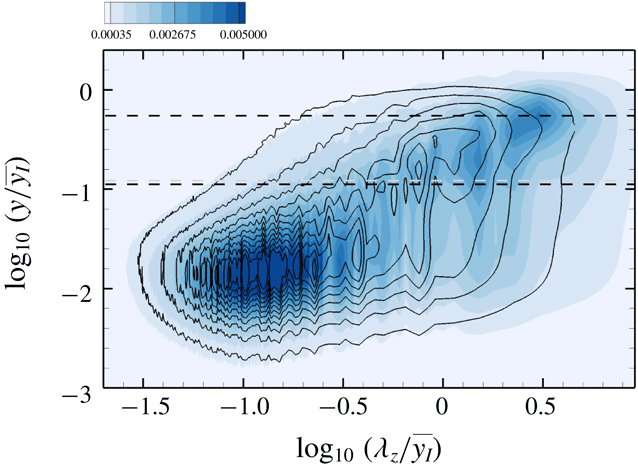
Numerous recent studies have examined the turbulent/non-turbulent interface in free and wall-bounded shear flows (e.g. Bisset, Hunt & Rogers Reference Bisset, Hunt and Rogers2002; Jiménez et al. Reference Jiménez, Hoyas, Simens and Mizuno2010; da Silva et al. Reference da Silva, Hunt, Eames and Westerweel2014; Borrell & Jiménez Reference Borrell and Jiménez2016; Lee et al. Reference Lee, Sung and Zaki2017). An effective approach is to define the interface as an iso-surface of vorticity magnitude which, if appropriately normalized, becomes independent of Reynolds number in spatially developing flows. Borrell & Jiménez (Reference Borrell and Jiménez2016) proposed the following normalization:
 $$\begin{eqnarray}\displaystyle |\unicode[STIX]{x1D714}|^{\ast }=\frac{|\unicode[STIX]{x1D714}|}{u_{\unicode[STIX]{x1D70F}}^{2}/\unicode[STIX]{x1D708}}\sqrt{\unicode[STIX]{x1D6FF}_{99}^{+}}. & & \displaystyle\end{eqnarray}$$
The threshold level,
 $|\unicode[STIX]{x1D714}|_{thres}^{\ast }$
, is then determined from the probability density function of the logarithm of
 $|\unicode[STIX]{x1D714}|^{\ast }$
, which is plotted in figure 6 for the inlet boundary layer. The two dashed lines in the figure were proposed by Lee et al. (Reference Lee, Sung and Zaki2017), and mark the wake regime and the geometric centre of the outer intermittent regime. Their intersection is the normalized vorticity threshold, here
 $|\unicode[STIX]{x1D714}|_{thres}^{\ast }=0.2$
, and the associated wall-normal height is
 $y/\unicode[STIX]{x1D6FF}_{99}\sim 1.0$
. In conventional boundary layers below a quiescent free stream, the turbulent/non-turbulent interface separates vortical flow (
 $|\unicode[STIX]{x1D714}|^{\ast }>|\unicode[STIX]{x1D714}|_{thres}^{\ast }$
) and irrotational flow (
 $|\unicode[STIX]{x1D714}|^{\ast }<|\unicode[STIX]{x1D714}|_{thres}^{\ast }$
). The method can be adopted in reference simulation where the TBL is beneath a quiescent free stream, but is not applicable when the free stream is itself turbulent.
Probability density function of
 $\log _{10}|\unicode[STIX]{x1D714}|^{\ast }$
at inlet (
 $Re_{\unicode[STIX]{x1D703}}\approx 1200$
). Dashed lines identify the wake regime of the boundary layer and the geometric centre of outer intermittent flow regime.

Another approach to differentiate the boundary layer and free stream is inspired by experiments in high-Prandtl-number fluids, where one stream is heated (Hancock & Bradshaw Reference Hancock and Bradshaw1989). In the simulations, a scalar marker can be set to unity in the boundary layer and zero in the free stream at the inflow plane. In the case of a conventional boundary layer, diffusion of the scalar is effective within the boundary layer only, and a value of zero guarantees that the scalar is associated with the free stream. But when the free stream is turbulent, diffusion becomes appreciable on both sides of the interface, and it once again becomes difficult to separate the boundary-layer and free-stream fluids. In order to remedy this effect, in numerical simulations, we eliminate diffusion altogether and adopt a level-set approach for capturing the interface (Jung & Zaki Reference Jung and Zaki2015).
In the original work by Osher & Sethian (Reference Osher and Sethian1988), the interface is an iso-level of the function
 $\unicode[STIX]{x1D711}$
that is tracked by solving
 $$\begin{eqnarray}\displaystyle \frac{\unicode[STIX]{x2202}\unicode[STIX]{x1D711}}{\unicode[STIX]{x2202}t}+\frac{\unicode[STIX]{x2202}u_{j}\unicode[STIX]{x1D711}}{\unicode[STIX]{x2202}x_{j}}=0. & & \displaystyle\end{eqnarray}$$
The value of
 $\unicode[STIX]{x1D711}$
is the unit distance from the interface, which is marked by
 $\unicode[STIX]{x1D711}=0$
. Since mass conservation is difficult to maintain in the original formulation, Desjardins, Moureau & Pitsch (Reference Desjardins, Moureau and Pitsch2008) proposed a conservative level-set method. Instead of solving for the evolution of
 $\unicode[STIX]{x1D711}$
, their approach utilizes a hyperbolic tangent function
 $$\begin{eqnarray}\displaystyle \unicode[STIX]{x1D713}=\frac{1}{2}\left(\tanh \left(\frac{\unicode[STIX]{x1D711}}{2\unicode[STIX]{x1D716}}\right)+1\right), & & \displaystyle\end{eqnarray}$$
where
 $\unicode[STIX]{x1D713}=0.5$
marks the interface location and
 $\unicode[STIX]{x1D716}\equiv 0.5\min (\unicode[STIX]{x0394}x,\unicode[STIX]{x0394}y,\unicode[STIX]{x0394}z)$
determines its thickness. The evolution of
 $\unicode[STIX]{x1D713}$
is given by
 $$\begin{eqnarray}\displaystyle \frac{\unicode[STIX]{x2202}\unicode[STIX]{x1D713}}{\unicode[STIX]{x2202}t}+\frac{\unicode[STIX]{x2202}u_{j}\unicode[STIX]{x1D713}}{\unicode[STIX]{x2202}x_{j}}=0. & & \displaystyle\end{eqnarray}$$
In order to maintain a smooth
 $\unicode[STIX]{x1D713}$
field, without spurious oscillations, a reinitialization equation is required:
 $$\begin{eqnarray}\displaystyle \frac{\unicode[STIX]{x2202}\unicode[STIX]{x1D713}}{\unicode[STIX]{x2202}\unicode[STIX]{x1D70F}}+\unicode[STIX]{x1D735}\boldsymbol{\cdot }(\unicode[STIX]{x1D713}(1-\unicode[STIX]{x1D713})\boldsymbol{n})=\unicode[STIX]{x1D735}\boldsymbol{\cdot }(\unicode[STIX]{x1D716}(\unicode[STIX]{x1D735}\unicode[STIX]{x1D713}\boldsymbol{\cdot }\boldsymbol{n})\boldsymbol{n}), & & \displaystyle\end{eqnarray}$$
where
 $\unicode[STIX]{x1D70F}$
is a pseudo-time step and
 $\boldsymbol{n}\equiv \unicode[STIX]{x1D735}\unicode[STIX]{x1D713}/|\unicode[STIX]{x1D735}\unicode[STIX]{x1D713}|$
is the interface normal vector. Note that
 $\boldsymbol{n}$
is computed from
 $\unicode[STIX]{x1D711}$
. When the reinitialization equation is invoked, it is solved to a steady state in pseudo-time, which requires three to four iterations in our simulations.
Time integration of (3.4) and (3.5) was performed using the third-order total variation diminishing Runge–Kutta scheme. The advection term in (3.4) was discretized in space using a fifth-order upstream central scheme, while second-order central differencing was adopted for the compression and diffusion terms in (3.5). In order to accelerate the computation, the level-set equations are solved in a narrow band around the interface only (Peng et al. Reference Peng, Merriman, Osher, Zhao and Kang1999). Extensive validation of the interface tracking algorithm was reported by Jung & Zaki (Reference Jung and Zaki2015), who computed the evolution of the Zalesak disc (Zalesak Reference Zalesak1979) and the evolution of linear and nonlinear instability waves in two-fluid flows (Cheung & Zaki Reference Cheung and Zaki2010, Reference Cheung and Zaki2011).
At the inflow plane, the value of
 $\unicode[STIX]{x1D713}$
is set to unity in the boundary layer and zero in the free stream, and is a hyperbolic tangent profile within five computational cells that straddle the interface. The instantaneous location of the interface, within the inlet boundary-layer data, is identified using the vorticity threshold
 $|\unicode[STIX]{x1D714}|_{thres}^{\ast }=0.2$
, and is assigned the value
 $\unicode[STIX]{x1D713}=0.5$
. Downstream, a sharp interface is maintained by virtue of the reinitialization equation. The indicator function, used in the conditional sampling, is thus defined as
 $\unicode[STIX]{x1D6E4}=1$
when
 $\unicode[STIX]{x1D713}\geqslant 0.5$
in the boundary-layer fluid and as
 $\unicode[STIX]{x1D6E4}=0$
when
 $\unicode[STIX]{x1D713}<0.5$
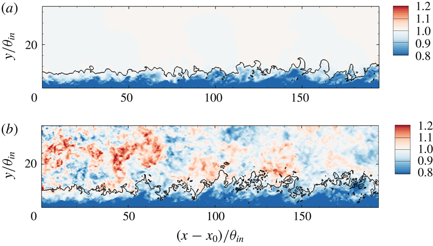
in the free stream. A sample result is shown in figure 7, where the interface
 $\unicode[STIX]{x1D713}=0.5$
is plotted along with contours of the streamwise velocity. Using
 $\unicode[STIX]{x1D713}=0.5$
, we can unambiguously differentiate the boundary-layer turbulence and FST and perform conditional sampling.
3.1 Comparison of conditional sampling using
 $|\unicode[STIX]{x1D714}|_{thres}^{\ast }$
and
$\unicode[STIX]{x1D713}$


The vorticity threshold and the level-set approaches identify two different interfaces. The former marks the outer diffusive edge of the boundary layer, while the latter marks the material fluid that belongs to the boundary layer at the inlet. Previous studies of conventional boundary layers, with quiescent free streams, have used the vorticity threshold. Since it is not applicable in the presence of FST, we will adopt the level-set method throughout this work. A comparison of both techniques is, nonetheless, possible in the reference case without FST.
Contours of streamwise velocity
 $u$
, the line identifying the level set
 $\unicode[STIX]{x1D713}=0.5$
, in TBL (a) without and (b) with FST.

Mean streamwise velocity profiles in inner scaling at (a)
 $Re_{\unicode[STIX]{x1D703}}=1900$
and (b)
 $Re_{\unicode[STIX]{x1D703}}=3000$
in REF case. (——) Conventional mean; (– – –) boundary-layer contribution; (— ⋅ —) free-stream contribution. Conditional statistics are evaluated using (black) vorticity threshold
 $|\unicode[STIX]{x1D714}|$
and (grey) level set function
 $\unicode[STIX]{x1D713}$
. The thin dashed line is given by
 $\overline{u}^{+}=2.44\ln (y^{+})+5.2$
.

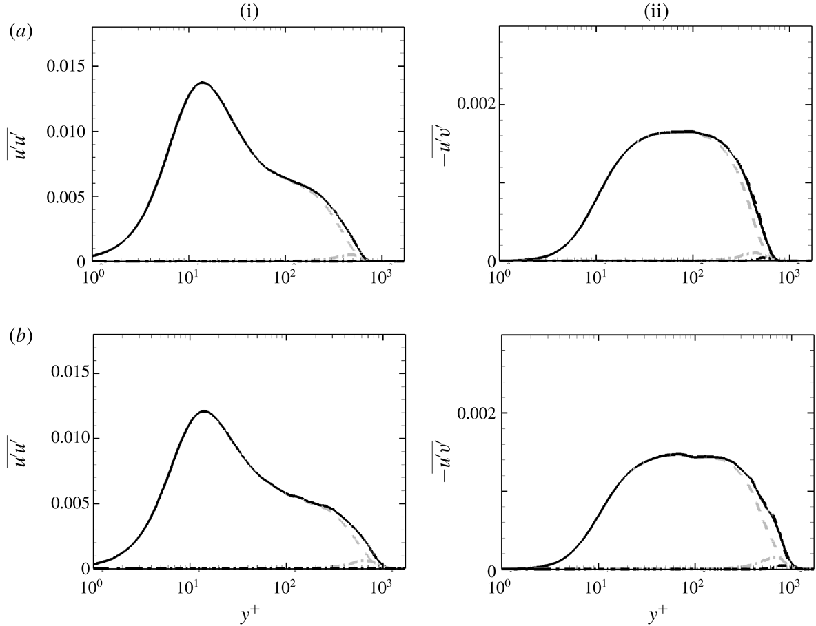
Reynolds stress profiles at (a)
 $Re_{\unicode[STIX]{x1D703}}=1900$
and (b)
 $Re_{\unicode[STIX]{x1D703}}=3000$
in REF case; (i)
 $\overline{u^{\prime }u^{\prime }}$
and (ii)
 $-\overline{u^{\prime }v^{\prime }}$
, both normalized by
 $U_{\infty }^{2}$
. Other details as in figure 8.

Figure 8 shows the mean velocity profiles at two different streamwise locations in the reference simulation. In addition to the conventional mean, the figure also shows the conditional averages in the boundary layer,
 $\unicode[STIX]{x1D6FE}\overline{u}^{+B}$
, and in the free stream,
 $(1-\unicode[STIX]{x1D6FE})\overline{u}^{+F}$
. The conditional curves are plotted twice, using the vorticity threshold (black) and the level-set approach (grey). Considering the free-stream contribution, it decays faster into the boundary layer when evaluated using the vorticity threshold relative to the level-set approach. In the former case, free-stream fluid that becomes part of the boundary layer as it diffuses only contributes to the boundary-layer statistics. In the level-set case, however, fluid that is assigned to the free stream at the inlet continues to contribute to the free-stream statistics even if it became part of the TBL. It is important to note that, at both downstream locations considered, the log-law region is fully captured by the boundary-layer conditional average, independent of the sampling technique.
The boundary-layer and free-stream contributions to the Reynolds stresses, evaluated using both the vorticity threshold and the level-set approach, are plotted in figure 9. The boundary-layer term
 $\unicode[STIX]{x1D6FE}\overline{u_{i}^{\ast }u_{j}^{\ast }}$
traces the conventional average from the wall through the inner peak and the log-law region. When
 $|\unicode[STIX]{x1D714}|_{thres}^{\ast }$
is used for conditional averaging, the free-stream contribution
 $(1-\unicode[STIX]{x1D6FE})\overline{u_{i}^{\prime \prime }u_{j}^{\prime \prime }}$
is essentially negligible even in the wake region. When
 $\unicode[STIX]{x1D713}$
is used, the free-stream contribution is small, and increases slightly downstream as more outer fluid becomes turbulent. Throughout the rest of this study, the level-set method will be adopted to evaluate conditional statistics, since it is equally applicable when the boundary layer is beneath a quiescent or turbulent free stream.
3.2 Statistics of the interface
The interface between the boundary layer and the free stream is defined as
 $y_{I}\equiv y(\unicode[STIX]{x1D713}=0.5)$
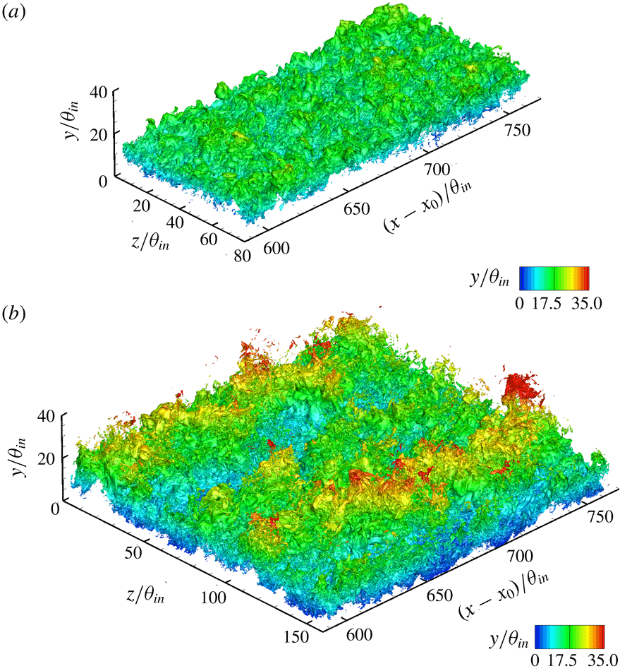
. Iso-surfaces of this quantity are plotted in figure 10, coloured by distance from the wall over a limited streamwise range. The figure qualitatively shows that the presence of the FST significantly enhances the undulation of the interface, relative to a canonical boundary layer.
Iso-surfaces of
 $y_{I}$
coloured by wall-normal height
 $y/\unicode[STIX]{x1D703}_{in}$
. (a) REF case and (b) FRC case.

(a) Downstream evolution of (——)
 $\overline{y_{I}}$
, (–
 $\times$
–)
 $\overline{y_{I}}^{+}$
and (– – –)
 $\unicode[STIX]{x1D6FF}_{99}$
. (b) Evolution of (——)
 $y_{I,rms}^{\prime }$
and (– – –)
 $y_{I,rms}^{\prime }/\overline{y_{I}}$
. Grey: REF case; black: FRC case.

Figure 11(a) contrasts the downstream development of the mean height of the interface,
 $\overline{y_{I}}$
, and the
 $99\,\%$
thickness of the boundary layer,
 $\unicode[STIX]{x1D6FF}_{99}$
. By construction, both quantities start at the same height at the inlet plane since
 $\unicode[STIX]{x1D713}=0.5$
was instantaneously assigned based on the vorticity threshold
 $|\unicode[STIX]{x1D714}|_{thres}^{\ast }=0.2$
(see figure 6). For the reference boundary layer (grey lines), both
 $\overline{y_{I}}$
and
 $\unicode[STIX]{x1D6FF}_{99}$
grow at similar rates, although the latter is slightly higher because the growing boundary layer entrains free-stream fluid. The results for the forced case show a steeper increase in
 $\unicode[STIX]{x1D6FF}_{99}$
, which was noted in previous studies (Hancock & Bradshaw Reference Hancock and Bradshaw1989). Note, however, that
 $\unicode[STIX]{x1D6FF}_{99}$
bears no physical significance, and is sensitive to the details of the mean velocity profile. On the other hand,
 $\overline{y_{I}}$
is the mean height of the material line separating the boundary layer from the free stream at the inlet. This quantity has a much smoother evolution with downstream distance, and shows only a moderate increase relative to the reference case.
The excursions of the interface relative to the mean location are measured by the root-mean-square of the fluctuations in its height,
 $y_{I,rms}^{\prime }$
, in figure 11(b). Lee et al. (Reference Lee, Sung and Zaki2017) showed that
 $y_{I,rms}^{\prime }$
increases with downstream distance, and is nearly linearly proportional to
 $\overline{y_{I}}$
in TBLs. The same trend is observed in the reference flow, where
 $y_{I,rms}^{\prime }/\overline{y_{I}}$
is nearly flat in figure 11(b). When the boundary layer is forced by FST, the root-mean-square of the interface excursions increases significantly. When normalized by
 $\overline{y_{I}}$
, it still shows an initial increase before it plateaus. The larger excursions in the interface height correspond to enhanced transport at the interface.
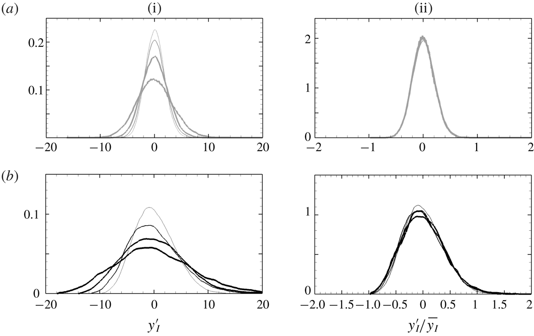
Probability density function of (i)
 $y_{I}^{\prime }$
and (ii)
 $y_{I}^{\prime }/\overline{y_{I}}$
for (a) REF case and (b) FRC case. Thin to thick lines correspond to the streamwise position,
 $(x-x_{0})/\unicode[STIX]{x1D703}_{in}=\{100,200,400,800\}$
.

The probability density function of the interface excursions is plotted in figure 12. The distributions for each flow nearly collapse when normalized by the mean value,
 $y_{I}^{\prime }/\overline{y_{I}}$
. In the reference boundary-layer simulation, the probability density function is practically symmetric, and its skewness at the shown locations is in the range
 $[0.12,0.15]$
. In the presence of free-stream forcing, the normalized probability density function curves are wider, and are more positively skewed in the direction of the free stream. Quantitatively, the skewness increases by as much as three-fold, and is in the range
 $[0.35,0.5]$
. Since
 $\overline{y_{I}}$
is larger in the forced case, the spread in the probability density function of
 $y^{\prime }$
is even more pronounced than in the reference case.
Due to the larger undulation of the interface height in the forced case, the intermittency
 $\unicode[STIX]{x1D6FE}$
spreads more rapidly as shown in the left-hand panel of figure 13. In the middle panels, wall-normal profiles for two streamwise positions are plotted versus
 $y/\overline{y_{I}}$
, and show good collapse in this outer scaling. When the boundary layer is buffeted by external disturbances, the profiles of
 $\unicode[STIX]{x1D6FE}$
clearly show its spread both towards the free stream and the wall. The FST is thus expected to influence the flow deep inside the mean shear. The extent of its penetration should, however, be viewed in inner scaling as shown in the rightmost panels. In the reference simulation, the contribution of the outer flow, or
 $(1-\unicode[STIX]{x1D6FE})$
, vanishes in the logarithmic layer. In the forced case, while the contribution of the free stream remains finite in the logarithmic layer, it is vanishingly small in the buffer layer.
4 Modification of boundary-layer statistics due to FST
4.1 The skin friction
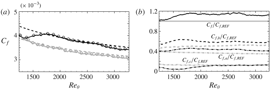
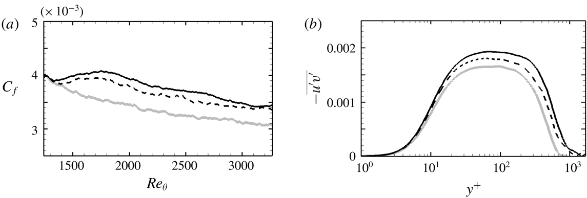
When TBLs are exposed to free-stream vortical forcing, the wall shear stress is enhanced. This effect is shown in figure 14(a) where the downstream evolution of the skin-friction coefficient,
 $C_{f}\equiv \unicode[STIX]{x1D70F}_{w}/(0.5\unicode[STIX]{x1D70C}U_{\infty }^{2})$
, is plotted versus the momentum-thickness Reynolds number. The coefficient increases by approximately
 $15\,\%$
at
 $Re_{\unicode[STIX]{x1D703}}=1900$
. Many of the subsequent discussions will be supported by results at this location and also
 $Re_{\unicode[STIX]{x1D703}}=3000$
farther downstream. Note that these Reynolds numbers do not correspond to the same streamwise positions in the reference and forced boundary layers (cf. figure 5). Matching
 $Re_{\unicode[STIX]{x1D703}}$
is, however, the appropriate choice for comparing the two flows. Hereafter, grey and black lines always indicate the profile of the reference and forced TBLs, respectively.
In figure 14(a), the
 $C_{f}$
curve is shifted upwards in presence of free-stream forcing, and retains its dependence on
 $Re_{\unicode[STIX]{x1D703}}$
. Similar to Esteban et al. (Reference Esteban, Dogan, Rodríguez-López and Ganapathisubramani2017), the correlation
 $C_{f}=2[\log (Re_{\unicode[STIX]{x1D703}})/0.384+C]^{-2}$
is used to match the data by adjusting
 $C$
. For the reference flow,
 $C=4.127$
is anticipated (Nagib, Chauhan & Monkewitz Reference Nagib, Chauhan and Monkewitz2007) and yields good agreement for the present data. The constant must be adjusted to
 $C=2.77$
in order to accurately capture the dependence of
 $C_{f}$
on
 $Re_{\unicode[STIX]{x1D703}}$
in the presence of FST.
An interpretation of the skin friction in terms of three physical phenomena was recently proposed by Renard & Deck (Reference Renard and Deck2016). In a frame moving with the free-stream speed
 $U_{\infty }$
, the flat plate is pulled to the left at
 $-U_{\infty }$
. In that setting, the skin-friction coefficient can be interpreted as of the average normalized power imparted by the wall motion onto the fluid, and is the sum of three contributions:
 $$\begin{eqnarray}\displaystyle C_{f,RD} & = & \displaystyle \underbrace{\frac{2}{U_{\infty }^{3}}\int _{0}^{\infty }\unicode[STIX]{x1D708}\left(\frac{\unicode[STIX]{x2202}\overline{u}}{\unicode[STIX]{x2202}y}\right)^{2}\,\text{d}y}_{C_{f,a}}+\underbrace{\frac{2}{U_{\infty }^{3}}\int _{0}^{\infty }-\overline{u^{\prime }v^{\prime }}\frac{\unicode[STIX]{x2202}\overline{u}}{\unicode[STIX]{x2202}y}\,\text{d}y}_{C_{f,b}}\nonumber\\ \displaystyle & & \displaystyle +\,\underbrace{\frac{2}{U_{\infty }^{3}}\int _{0}^{\infty }(\overline{u}-U_{\infty })\frac{\unicode[STIX]{x2202}}{\unicode[STIX]{x2202}y}\left(\frac{\overline{\unicode[STIX]{x1D70F}}}{\unicode[STIX]{x1D70C}}\right)\,\text{d}y}_{C_{f,c}},\end{eqnarray}$$
where
 $\overline{\unicode[STIX]{x1D70F}}/\unicode[STIX]{x1D70C}$
is the total shear stress. The term
 $C_{f,a}$
is the rate of dissipation of mean streamwise kinetic energy into heat,
 $C_{f,b}$
is the rate of production of turbulence kinetic energy and
 $C_{f,c}$
is the rate of change in the streamwise kinetic energy in the mean flow. The symbols in figure 14(a) show the reconstruction of the right-hand side of (4.1), which agrees with the direct evaluation of the skin friction from the gradient at the wall.
(i) Contours of intermittency
 $\unicode[STIX]{x1D6FE}$
near the inlet of the simulation domain. Profiles of
 $\unicode[STIX]{x1D6FE}$
(ii) in outer scaling and (iii) in inner scaling at (– – –)
 $Re_{\unicode[STIX]{x1D703}}=1900$
and (——)
 $Re_{\unicode[STIX]{x1D703}}=3000$
. (a) REF case and (b) FRC case.

(a) Skin-friction coefficients computed from (——) the wall shear stress
 $C_{f}=\unicode[STIX]{x1D70F}_{w}/(\unicode[STIX]{x1D70C}U_{\infty }^{2})/2$
and (○) the decomposition (4.1). Dashed lines are the correlation
 $C_{f}=2[\log (Re_{\unicode[STIX]{x1D703}})/0.384+C]^{-2}$
, where
 $C=4.127$
for REF and
 $C=2.77$
for FRC. (b) Contributions to the skin-friction coefficient normalized by
 $C_{f,REF}$
; (——)
 $C_{f}$
, (— ⋅ —)
 $C_{f,a}$
, (– – –)
 $C_{f,b}$
and (— ⋅ ⋅ —)
 $C_{f,c}$
. Grey: REF; black: FRC.

All the terms in the decomposition (4.1) are plotted in figure 14(b), normalized by the total friction coefficient from the reference boundary-layer simulation,
 $C_{f,REF}(Re_{\unicode[STIX]{x1D703}})$
. The term
 $C_{f,c}$
, which accounts for the streamwise energy in the mean flow, is the smallest contributor to the friction and is initially reduced in response to the FST but subsequently recovers. The overall increase in the friction coefficient is therefore due to the augmentations of
 $C_{f,a}$
and
 $C_{f,b}$
, namely the dissipation in the mean profile and the production of turbulence kinetic energy. Both involve
 $-\overline{u^{\prime }v^{\prime }}$
, although indirectly in the first term through the mean-flow distortion by the stress.
The integral in
 $C_{f,a}$
converges to
 $95\,\%$
of its total below
 $y^{+}=20$
and to
 $99\,\%$
by
 $y^{+}=100$
. Within the region
 $y^{+}<100$
, the change in
 $\unicode[STIX]{x2202}\overline{u}/\unicode[STIX]{x2202}y$
from its wall value is nearly equal to the Reynolds shear stress, and therefore the increase in
 $C_{f,a}$
when the boundary layer is forced is related to the increase in
 $\overline{-u^{\prime }v^{\prime }}$
. This relation is demonstrated by integrating the mean-momentum equation for a ZPG boundary layer from the wall to a height
 $y$
:
 $$\begin{eqnarray}\displaystyle \frac{1}{Re}\left\{\frac{\unicode[STIX]{x2202}\overline{u}}{\unicode[STIX]{x2202}y}-\left[\frac{\unicode[STIX]{x2202}\overline{u}}{\unicode[STIX]{x2202}y}\right]_{y=0}\right\}=\int _{y}\frac{\unicode[STIX]{x2202}(\overline{u}\,\overline{u})}{\unicode[STIX]{x2202}x}\,\text{d}y+\overline{u}\,\overline{v}+\overline{u^{\prime }v^{\prime }}. & & \displaystyle\end{eqnarray}$$
The above expression was evaluated for both the reference and forced flows, and the difference
 $(\bullet )_{FRC}-(\bullet )_{REF}$
is plotted in figure 15, at
 $Re_{\unicode[STIX]{x1D703}}=1900$
and
 $3000$
. The results demonstrate how changes in
 $\overline{-u^{\prime }v^{\prime }}$
indirectly impact the dissipation in the mean-velocity profile,
 $C_{f,a}$
.
The differences in (——)
 $(1/Re)(\unicode[STIX]{x2202}\overline{u}/\unicode[STIX]{x2202}y-\unicode[STIX]{x2202}\overline{u}/\unicode[STIX]{x2202}y|_{y=0})$
and in (– – –)
 $\overline{u^{\prime }v^{\prime }}$
in the reference and forced boundary layers. (a)
 $Re_{\unicode[STIX]{x1D703}}=1900$
; (b)
 $Re_{\unicode[STIX]{x1D703}}=3000$
.

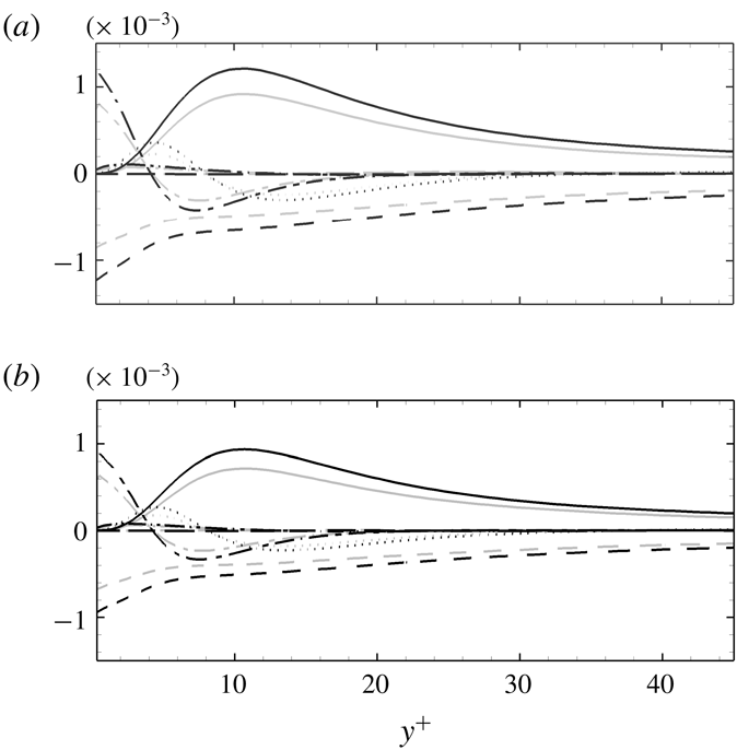
Wall-normal distributions of turbulence kinetic energy budget terms normalized by
 $U_{\infty }^{3}/\unicode[STIX]{x1D703}_{in}$
at (a)
 $Re_{\unicode[STIX]{x1D703}}=1900$
and (b)
 $Re_{\unicode[STIX]{x1D703}}=3000$
; (——) production
 ${\mathcal{P}}$
, (– – –) pseudo-dissipation
 $-\unicode[STIX]{x1D700}$
, (— ⋅ —) viscous diffusion
 ${\mathcal{D}}$
, (
 $\cdots \cdots$
) turbulent advection
 ${\mathcal{T}}$
, (— ⋅ ⋅ —) pressure diffusion
 ${\mathcal{R}}$
and (— —) mean advection
 ${\mathcal{A}}$
. Grey: REF; black: FRC.

The shear stress appears directly in
 $C_{f,b}$
whose increase signals a potential change in the energetics of the wall turbulence. Consider the kinetic energy budget
 $$\begin{eqnarray}\displaystyle \underbrace{\overline{u}_{j}\frac{\unicode[STIX]{x2202}k}{\unicode[STIX]{x2202}x_{j}}}_{{\mathcal{A}}}=-\underbrace{\overline{\frac{\unicode[STIX]{x2202}u_{i}^{\prime }p^{\prime }}{\unicode[STIX]{x2202}x_{i}}}}_{{\mathcal{R}}}\underbrace{-\frac{1}{2}\frac{\unicode[STIX]{x2202}\overline{u_{j}^{\prime }u_{i}^{\prime }u_{i}^{\prime }}}{\unicode[STIX]{x2202}x_{j}}}_{{\mathcal{T}}}\underbrace{-\overline{u_{i}^{\prime }u_{j}^{\prime }}\frac{\unicode[STIX]{x2202}\overline{u_{i}}}{\unicode[STIX]{x2202}x_{j}}}_{{\mathcal{P}}}-\underbrace{\frac{1}{Re}\overline{\frac{\unicode[STIX]{x2202}u_{i}^{\prime }}{\unicode[STIX]{x2202}x_{j}}\frac{\unicode[STIX]{x2202}u_{i}^{\prime }}{\unicode[STIX]{x2202}x_{j}}}}_{\unicode[STIX]{x1D700}}+\underbrace{\frac{1}{Re}\frac{\unicode[STIX]{x2202}^{2}k}{\unicode[STIX]{x2202}x_{j}\unicode[STIX]{x2202}x_{j}}}_{{\mathcal{D}}}, & & \displaystyle\end{eqnarray}$$
where
 $k\equiv (\overline{u_{i}^{\prime }u_{i}^{\prime }})/2$
is the turbulence kinetic energy per unit mass. In the above expression,
 ${\mathcal{A}}$
is mean advection,
 ${\mathcal{R}}$
is pressure-diffusion,
 ${\mathcal{T}}$
is turbulent advection,
 ${\mathcal{P}}$
is rate of production,
 $\unicode[STIX]{x1D700}$
is the pseudo-dissipation and
 ${\mathcal{D}}$
is viscous diffusion. These terms are plotted in the near-wall region in figure 16, and compared in the reference and forced boundary layers. The magnitude of every term is increased in the forced flow, especially the rate of dissipation and viscous diffusion at the wall. The production term is also appreciably increased in the buffer layer, which is consistent with the results of Péneau et al. (Reference Péneau, Boisson and Djilali2000). Based on the analysis by Renard & Deck (Reference Renard and Deck2016), in a frame moving with the free-stream speed
 $U_{\infty }$
, an increase of
 $\overline{u^{\prime }v^{\prime }}\unicode[STIX]{x2202}\overline{u}/\unicode[STIX]{x2202}y$
, and hence
 ${\mathcal{P}}$
, requires additional power input from the moving wall. This leads to an increase in wall shear stress, or drag. Further evidence of the connection between
 $\overline{u^{\prime }v^{\prime }}\unicode[STIX]{x2202}\overline{u}/\unicode[STIX]{x2202}y$
and drag is provided in figure 17. The wall-normal peak of the former term is plotted versus downstream Reynolds number, and its trend matches the change in the skin friction very well.
Evolutions of (——)
 $C_{f}$
and (▫) a peak value of
 $-\overline{u^{\prime }v^{\prime }}(\unicode[STIX]{x2202}\overline{u}/\unicode[STIX]{x2202}y)$
. Grey: REF; black: FRC.

A number of interesting lines of query arise from the above results. Firstly, the enhanced production in the buffer layer can be ascribed to either a change in the mean-flow profile or the Reynolds shear stresses. The two are not independent of one another, and which has a more pronounced effect is of interest. Secondly, the most pronounced change in the production term takes place in the buffer layer. Whether the FST penetrates this deep into the boundary layer or the near-wall turbulence dynamics are modified should be assessed. If the former, an increase in the shear stress is curious because the FST is isotropic; and the latter case would also warrant an explanation. These factors are examined by evaluating the contributions of the boundary-layer and free-stream fluids to the flow statistics.
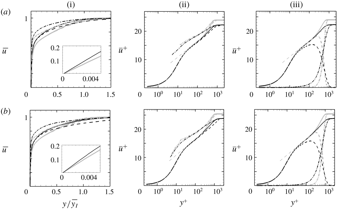
Profiles of mean streamwise velocity at (a)
 $Re_{\unicode[STIX]{x1D703}}=1900$
and (b)
 $Re_{\unicode[STIX]{x1D703}}=3000$
, normalized by (i)
 $U_{\infty }$
and (ii, iii)
 $u_{\unicode[STIX]{x1D70F}}$
. (i, ii) (– – –) Boundary-layer velocity
 $\overline{u}^{B}$
; (— ⋅ —) free-stream velocity
 $\overline{u}^{F}$
. (iii) (– – –) Boundary-layer contribution
 $\unicode[STIX]{x1D6FE}\overline{u}^{B}$
; (— ⋅ —) free-stream contribution
 $(1-\unicode[STIX]{x1D6FE})\overline{u}^{F}$
. The thin dashed line:
 $\overline{u}^{+}=2.44\ln (y^{+})+5.2$
. Grey: REF; black: FRC.

4.2 Conditional statistics
The mean streamwise velocity profiles are plotted in outer and inner scalings in figure 18, at
 $Re_{\unicode[STIX]{x1D703}}=1900$
and
 $3000$
. Note that the adopted outer length scale is
 $\overline{y_{I}}$
(left-hand panels), and not
 $\unicode[STIX]{x1D6FF}_{99}$
which does not bear a clear physical significance. The mean-velocity profiles are fuller in the FRC case, which is indicative of the enhanced mixing that was remarked upon by Hancock & Bradshaw (Reference Hancock and Bradshaw1989). It is also consistent with the increase in
 $C_{f,a}$
(4.1), which is the integral of
 $(\unicode[STIX]{x2202}\overline{u}/\unicode[STIX]{x2202}y)^{2}$
in the wall-normal direction, or dissipation of mean streamwise kinetic energy. The left-hand panels also show the conditional velocity profiles in the boundary layer,
 $\overline{u}^{B}$
, and in the free stream,
 $\overline{u}^{F}$
. These profiles, when weighted by their probabilities, make up the unconditional mean (2.14). Therefore they lie on either side of the mean, and agree with it near the wall and in the free stream, respectively. The free-stream conditional profile,
 $\overline{u}^{F}$
, is larger in the forced flow than in the reference case, but seems to only impact the mean profile near the outer edge of the boundary layer. It appears, at least based on outer scaling, that changes in the overall mean track the changes in the boundary-layer curve.
The middle panels of figure 18 show the same profiles in viscous scaling. Both the unforced and forced boundary layers have a logarithmic region,
 $\overline{u}^{+}=2.44\ln (y^{+})+5.2$
, at both Reynolds numbers. In the presence of FST, a significant depression of the boundary-layer profile occurs in the wake region, which is consistent with the increase in drag; the logarithmic, buffer and viscous regions are hardly affected. The unconditional mean profiles are thus consistent with earlier experiments (Hancock & Bradshaw Reference Hancock and Bradshaw1983; Sharp et al.
Reference Sharp, Neuscamman and Warhaft2009) and simulations (Li et al.
Reference Li, Schlatter and Henningson2010). The conditional profiles,
 $\overline{u}^{+B}$
and
 $\overline{u}^{+F}$
, are interesting. In both the reference and forced computations,
 $\overline{u}^{+B}$
faithfully follows the conventional mean up to the edge of the logarithmic layer, and is lower in the intermittent wake region. Conversely, the free-stream curves reproduce the outer uniform flow, retain a higher velocity than the conventional mean inside the boundary layer and collapse in viscous scaling. A deeper reach of
 $\overline{u}^{+F}$
towards the wall in the forced flow is evident in the figure. When weighted by their probabilities (right-hand panels), the conditional averages yield the contributions to the mean by the boundary layer,
 $\unicode[STIX]{x1D6FE}\overline{u}^{+B}$
, and the free stream,
 $(1-\unicode[STIX]{x1D6FE})\overline{u}^{+F}$
. In the unforced flow, the boundary-layer contributions still show a logarithmic-layer behaviour and decay sharply in the wake region due to the intermittency weighting. In contrast, when FST forcing is present, the boundary-layer contribution no longer traces the logarithmic law, although the logarithmic behaviour is re-established once the free-stream contribution is added to recover the conventional mean. In order to explain the ‘universality’, or robustness, of the logarithmic law in forced boundary layers, Hancock & Bradshaw (Reference Hancock and Bradshaw1989) verified that the departure from equilibrium is inappreciable, and that the rates of production and dissipation of turbulence kinetic energy are dominant and nearly balance in that region. The same dominant balance was verified in the present FRC case.
Reynolds stresses profiles at (a)
 $Re_{\unicode[STIX]{x1D703}}=1900$
and (b)
 $Re_{\unicode[STIX]{x1D703}}=3000$
: (i)
 $\overline{u^{\prime }u^{\prime }}$
; (ii)
 $\overline{v^{\prime }v^{\prime }}$
; (iii)
 $\overline{w^{\prime }w^{\prime }}$
; (iv)
 $-\overline{u^{\prime }v^{\prime }}$
, all normalized by
 $U_{\infty }^{2}$
. (——) Conventional statistics; (– – –) boundary-layer contribution; (— ⋅ —) free-stream contribution. Grey: REF; black: FRC.

Wall-normal profiles of Reynolds stresses are presented in figure 19. In general, all the stresses are enhanced when the boundary layer is subjected to FST and, outside the mean shear, all the normal stresses match the outer turbulence levels and the shear stress is nearly zero. Two key observation are important to note, related to the stresses in the logarithmic and buffer layers, respectively. Firstly, the increase in
 $\overline{u^{\prime }u^{\prime }}$
in the logarithmic layer exceeds the free-stream value, and is therefore not a mere upward shift of the curve. Partial evidence of enhanced local production of
 $\overline{u^{\prime }u^{\prime }}$
is available from the Reynolds shear stress,
 $\overline{u^{\prime }v^{\prime }}$
, which is increased in the logarithmic layer. This trend is curious, and cannot be directly ascribed to the FST since it is itself void of
 $\overline{u^{\prime }v^{\prime }}$
. Instead, the increase in normal stresses
 $\overline{v^{\prime }v^{\prime }}$
due to the ingested FST acts against the mean shear to produce Reynolds shear stress that, in turn, enhances the production of
 $\overline{u^{\prime }u^{\prime }}$
. Profiles of the relevant production terms,
 ${\mathcal{P}}_{u_{i}^{\prime }u_{j}^{\prime }}\equiv -\overline{u_{j}^{\prime }u_{k}^{\prime }}\unicode[STIX]{x2202}\overline{u_{i}}/\unicode[STIX]{x2202}x_{k}-\overline{u_{i}^{\prime }u_{k}^{\prime }}\unicode[STIX]{x2202}\overline{u_{j}}/\unicode[STIX]{x2202}x_{k}$
, are provided in figure 20, pre-multiplied by
 $y^{+}$
. In this form, the area under the curve corresponds to the integral of production, which is clearly enhanced in the logarithmic layer. The symbols identify the dominant contributions, and confirm that
 $\overline{v^{\prime }v^{\prime }}$
leads to an increase in production of the shear stress and, in turn, production of
 $\overline{u^{\prime }u^{\prime }}$
in the outer layer.
Profiles of production of Reynolds shear and streamwise-normal stresses at
 $Re_{\unicode[STIX]{x1D703}}=1900$
: (a)
 $y^{+}{\mathcal{P}}_{-u^{\prime }v^{\prime }}$
; (b)
 $y^{+}{\mathcal{P}}_{u^{\prime }u^{\prime }}$
. Symbols mark the leading contributions: (a)
 $y^{+}\overline{v^{\prime }v^{\prime }}\unicode[STIX]{x2202}\overline{u}/\unicode[STIX]{x2202}y$
; (b)
 $-2y^{+}\overline{u^{\prime }v^{\prime }}\unicode[STIX]{x2202}\overline{u}/\unicode[STIX]{x2202}y$
. Production terms are normalized by
 $U_{\infty }^{3}/\unicode[STIX]{x1D703}_{in}$
. Grey: REF; black: FRC.

The second observation from figure 19 concerns the depth towards the wall over which the Reynolds stress profiles are altered in the presence of FST. The increase in
 $\overline{v^{\prime }v^{\prime }}$
diminishes as we approach the wall and nearly vanishes within the buffer layer, which is consistent with the extent of penetration of FST into the boundary layer and the decay of the intermittency curves (see figure 13). In contrast, the increases in the other stresses preserve their magnitudes deeper into the boundary layer, beyond the decay of the intermittency curves. For example, the increases in the streamwise and spanwise normal stresses are evident below the locations of their respective peaks, and even deeper than the buffer layer. Therefore, these changes cannot be caused by the FST directly, and the explanation for enhanced production in the logarithmic layer does not carry over to the buffer region. This point is further supported by the conditional free-stream contributions,
 $(1-\unicode[STIX]{x1D6FE})\overline{u_{i}^{\prime \prime }u_{j}^{\prime \prime }}^{F}$
, which vanish farther away from the wall than the increase in the stresses. In summary, while the FST has a direct contribution to the normal stresses in the outer intermittent region and enhances production of
 $\overline{u^{\prime }v^{\prime }}$
and
 $\overline{u^{\prime }u^{\prime }}$
in the logarithmic layer, it also indirectly modifies the turbulence deeper towards the wall in a manner that warrants further examination – a matter that we address in § 5.
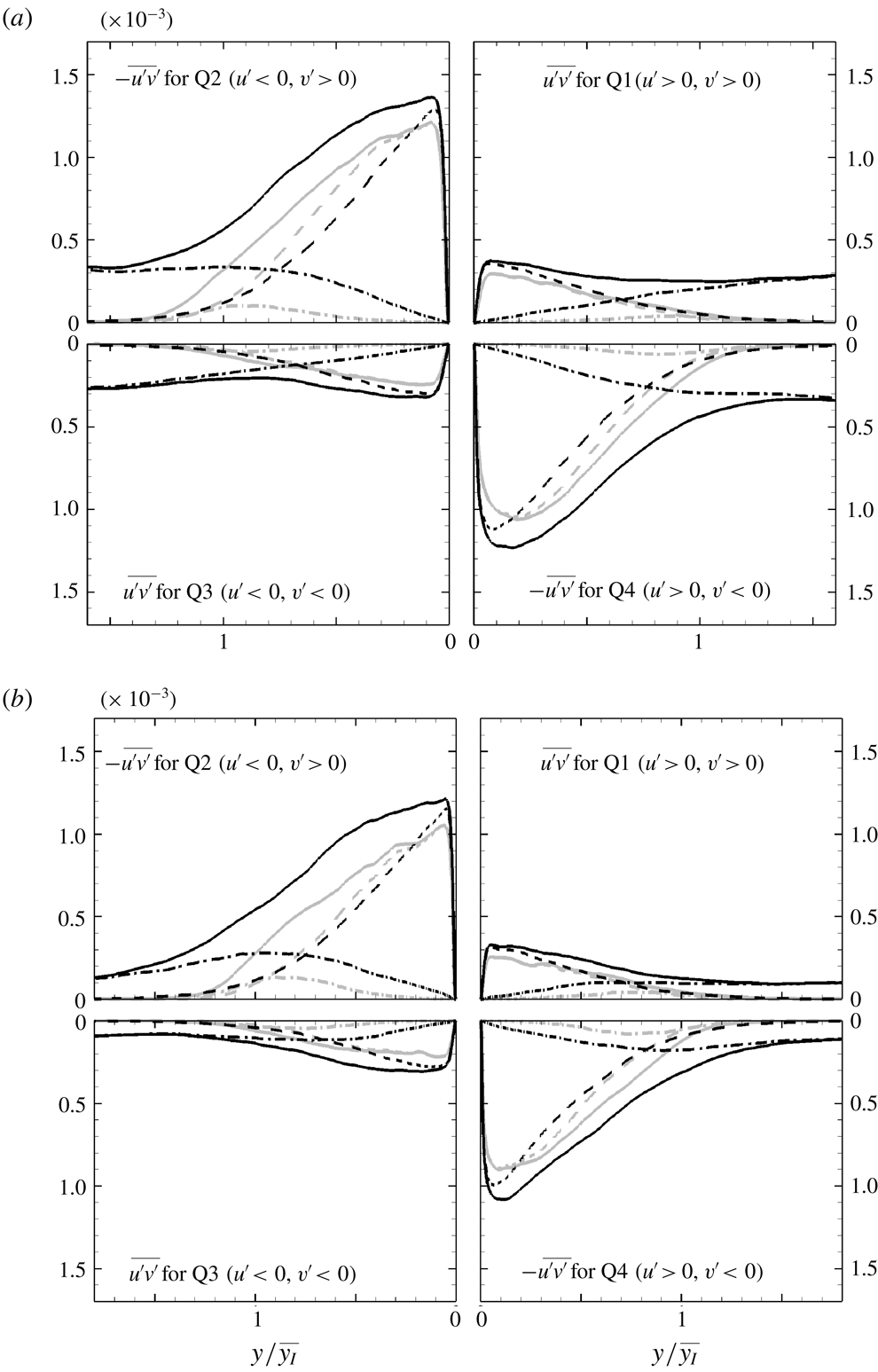
Contributions to Reynolds shear stress,
 $-\overline{u^{\prime }v^{\prime }}$
normalized by
 $U_{\infty }^{2}$
, from each quadrant at (a)
 $Re_{\unicode[STIX]{x1D703}}=1900$
and (b)
 $Re_{\unicode[STIX]{x1D703}}=3000$
. (——) Conventional statistics; (– – –) boundary-layer contribution; (— ⋅ —) free-stream contribution. Grey: REF; black: FRC.

The increase in production is connected to the changes in Reynolds shear stress within the boundary layer. The cross-correlation coefficient,
 $\overline{u^{\prime }v^{\prime }}/(u_{rms}^{\prime }v_{rms}^{\prime })$
, is reduced in the presence of external forcing because the isotropy of the FST destroys the coherence of the boundary-layer turbulence (Hancock & Bradshaw Reference Hancock and Bradshaw1989). Nonetheless, the magnitude of Reynolds shear stress
 $\overline{u^{\prime }v^{\prime }}$
increases in the boundary layer as shown in figure 19, and as reported by others (Péneau et al.
Reference Péneau, Boisson and Djilali2000). This increase is curious because the free-stream forcing is free of any mean shear stress, and because the extent of its penetration into the mean shear, towards the wall, is shallower than the region of increase in kinetic energy and production which persist deeper towards the wall.
A more detailed account of the increase in the Reynolds shear stress can be obtained from quadrant analysis (Wallace Reference Wallace2016). The analysis was performed for both the reference and forced flows, and is shown in figure 21 at the two downstream locations,
 $Re_{\unicode[STIX]{x1D703}}=1900$
and
 $3000$
. In the reference flow, ejection (Q2:
 $u^{\prime }<0$
and
 $v^{\prime }>0$
) and sweep (Q4:
 $u^{\prime }>0$
and
 $v^{\prime }<0$
) events are dominant (figure 21). In the forced case, the isotropy of FST leads to finite, nearly equal contribution to all four quadrants at and beyond the free-stream edge of the boundary layer, thus enhancing mixing in that region. Inside the boundary layer, the increases in Q2 and Q4 events far exceed those in the other two components. In addition, while the free-stream contribution decays within the boundary layer, a significant increase in the unconditional Q2 and Q4 events is observed near their respective peaks close to the wall. The peak of the boundary-layer contribution, which resides close to the wall, increases in magnitude but its location does not shift. The more pronounced ejections and sweeps are consistent with the higher rate of production,
 $P_{-u^{\prime }v^{\prime }}$
, in the forced case (figure 20
a).
Profiles of (i) pseudo-dissipation
 $\unicode[STIX]{x1D700}$
and (ii) production
 ${\mathcal{P}}$
terms, both normalized by
 $U_{\infty }^{3}/\unicode[STIX]{x1D703}_{in}$
. (a)
 $Re_{\unicode[STIX]{x1D703}}=1900$
; (b)
 $Re_{\unicode[STIX]{x1D703}}=3000$
. (——) Conventional statistics; (– – –) boundary-layer contribution; (— ⋅ —) free-stream contribution. Grey: REF; black: FRC.

Figure 22 highlights the change in the near-wall turbulence kinetic energy production and dissipation rates and their conditional contributions, all plotted in logarithmic scale. The relationship between the conventional and conditional terms is provided in appendix A. In the reference simulation, the dissipation is zero in the free stream, and its high level near the wall is entirely due to the boundary-layer contribution. In the forced case, the dissipation is enhanced throughout the extent of the boundary layer and is finite, albeit small, in the free stream where it is entirely due to the contribution of the outer fluid. The free-stream conditional average decays inside the boundary layer and is more than two orders of magnitude smaller than the boundary-layer counterpart. Similar observations are applicable to the production terms. In this case, however, the free-stream contribution vanishes outside the mean shear in both the reference and forced configurations. While it is enhanced inside the boundary layer when the flow is forced, that contribution remains more than two orders of magnitude smaller than the peak value of the total production. The increase in production near the wall
 $(y^{+}\simeq 10)$
in the forced flow is essentially entirely due to the boundary-layer contribution. These results are consistent with the notion that the increase in the peak Reynolds stresses (figure 19), especially
 $\overline{u^{\prime }u^{\prime }}$
, is not an additive effect of injection of FST into the near-wall region. Instead, the turbulence kinetic energy and its production rate are enhanced near the wall, below the extent of penetration of free-stream perturbations. The associated changes in the structures and spectra of the wall turbulence are examined in § 5.
4.3 Discussion
The arguments set forth so far in order to explain the increase in the boundary-layer turbulence kinetic energy in the forced flow have focused on changes in the near-wall dynamics. Another potential factor is an influx of turbulence from the free stream. This effect was considered by Hancock & Bradshaw (Reference Hancock and Bradshaw1989), who evaluated the conditionally sampled turbulent fluxes. They concluded that the net flux is into the boundary layer, but their conditional sampling method relied on a diffusive scalar and they computed the perturbations relative to the unconditional mean. The present configuration is different, as we illustrate by considering the instantaneous total kinetic energy,
 $K\equiv (u_{i}u_{i})/2$
. The instantaneous flux of
 $K$
relative to the interface is given by
 $\int _{S_{I}}K(u_{j}-v_{j})n_{j}\,\text{d}S_{I}$
, where
 $S_{I}$
is the surface of the interface and
 $v_{j}$
and
 $n_{j}$
are its velocity and outward unit-normal vectors. The instantaneous flux term is identically zero because the interface is a material line,
 $v_{j}=u_{j}$
. In other words, free-stream energy is not advected across the interface – a condition that is unique to our configuration because the interface is a material line – and energy flux does not contribute to the reported changes in boundary-layer turbulence.
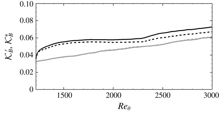
Average of the integrated perturbation kinetic energy inside the boundary layer: (——)
 $\!{\mathcal{K}}_{B}^{\prime }=\overline{\int _{0}^{\infty }(\unicode[STIX]{x1D6E4}/2)u_{i}^{\prime }u_{i}^{\prime }\,\text{d}y}$
; (– – –)
 $\!{\mathcal{K}}_{B}^{\ast }=\overline{\int _{0}^{\infty }(\unicode[STIX]{x1D6E4}/2)u_{i}^{\ast }u_{i}^{\ast }\,\text{d}y}$
. Grey: REF; black: FRC.

Another point to note is the contribution of intermittency to the change in the total turbulence kinetic energy within the boundary layer. Figure 23 compares
 ${\mathcal{K}}_{B}^{\prime }=\overline{\int _{0}^{\infty }(\unicode[STIX]{x1D6E4}/2)u_{i}^{\prime }u_{i}^{\prime }\,\text{d}y}$
and
 ${\mathcal{K}}_{B}^{\ast }=\overline{\int _{0}^{\infty }(\unicode[STIX]{x1D6E4}/2)u_{i}^{\ast }u_{i}^{\ast }\,\text{d}y}$
. Both quantities are evaluated within the boundary-layer fluid only, before averaging. The first term features the kinetic energy of perturbations relative to the conventional mean and the second is relative to the conditional mean. Their near perfect agreement for the reference simulation (figure 23) demonstrates that the conventional and conditional means are similar within the boundary-layer fluid, over the wall-normal extent where turbulence is energetic and makes up the majority of the integral. The two quantities deviate in the forced flow, because the intermittency profiles spread deeper towards the wall, but nonetheless their relative difference remains small,
 $4.9\,\%$
at
 $Re_{\unicode[STIX]{x1D703}}=1900$
and
 $7.5\,\%$
at
 $Re_{\unicode[STIX]{x1D703}}=3000$
. Therefore, the direct contribution of intermittency is small in regions within the boundary layer where the Reynolds normal stresses are increased appreciably.
Based on the present discussion, the choice of the interface as a material line precludes flux of energy from the free stream into the boundary layer. In addition, the overall increase in the turbulence kinetic energy within the boundary layer takes place largely below the region influenced by intermittency. Both points provide support to the notion that the increase in the turbulence kinetic energy inside the boundary layer is due to a change in the dynamics of the wall flow. The corresponding changes in turbulence spectra and structures are the focus of § 5.
5 Turbulence structures
The increases in the Reynolds streamwise stress in the logarithmic layer and the near-wall region are the outcome of changes in the turbulence structures when the boundary layer is forced by FST. A realization of the large-scale motions in the logarithmic layer is shown in figure 24, visualized using iso-surfaces of the Gaussian-filtered streamwise velocity perturbations (see Lee et al. Reference Lee, Sung and Zaki2017, for details of the structure identification procedures). The figure empirically suggests that the large-scale motions are wider in the span and more elongated in the streamwise direction when the flow is forced. The enhanced coherence of the energetic structures is interesting, in particular since the FST is isotropic. In this section, we will quantify the change in the size of these large-scale structures, their spectral signature and their impact on the near-wall turbulence.
Iso-surfaces of the Gaussian-filtered flow field
 $\hat{u} ^{\prime }$
. (a) REF case and (b) FRC case. Blue:
 $\hat{u} ^{\prime }=-0.06$
; red:
 $\hat{u} ^{\prime }=0.06$
.

In order to quantify the change in the size of the energetic large-scale structures, the two-point correlation coefficient for streamwise velocity fluctuations is computed:
 $$\begin{eqnarray}\displaystyle {R_{u^{\prime }u^{\prime }}}_{(\unicode[STIX]{x0394}x,y,\unicode[STIX]{x0394}z)}=\frac{\overline{u_{(x,y_{ref},z,t)}^{\prime }u_{(x+\unicode[STIX]{x0394}x,y,z+\unicode[STIX]{x0394}z,t)}^{\prime }}}{u_{rms(x,y_{ref})}^{\prime }~u_{rms(x,y)}^{\prime }}, & & \displaystyle\end{eqnarray}$$
where
 $y_{ref}$
is the reference wall-normal location. Contours of
 $R_{u^{\prime }u^{\prime }}$
are plotted in figure 25; line contours correspond to the reference flow and the flood contours correspond to the forced case. The figure also shows the correlation in the
 $45^{\circ }$
and
 $135^{\circ }$
inclined planes. In all three views, the correlation coefficient is appreciably wider in the forced flow, which demonstrates that the
 $u$
-perturbation structures in the logarithmic layer are larger in streamwise, spanwise and wall-normal extent. Two characteristic length scales,
 $l_{45^{\circ }}$
and
 $l_{135^{\circ }}$
, are evaluated from the inclined planes, and are defined as the distance to
 $R_{u^{\prime }u^{\prime }}=0.5$
. Their ratio in the reference case is
 $l_{45^{\circ }}/l_{135^{\circ }}=1.2$
, which agrees with the value reported by Ganapathisubramani et al. (Reference Ganapathisubramani, Hutchins, Hambleton and Longmire2005). Those authors attributed the fact that
 $l_{45^{\circ }}$
is greater than
 $l_{135^{\circ }}$
to the existence of hairpin packets. In the forced flow, the ratio increases to
 $l_{45^{\circ }}/l_{135^{\circ }}=1.27$
, which is consistent with enhanced hairpin activity. Geometrically, the increase in
 $l_{45^{\circ }}/l_{135^{\circ }}$
can arise due to a steeper inclination angle,
 $\unicode[STIX]{x1D6FC}$
, or larger aspect ratio of the structures,
 $AR=l_{long}/l_{short}$
, where
 $l_{long}$
and
 $l_{short}$
are the longest and shortest lengths in the
 $x$
–
 $y$
plane. Both quantities are plotted in figure 26 as a function of the threshold level of the correlation coefficient,
 $R_{thres}$
, that is adopted to define the size of the structure. The inclination angle is similar in both cases, and hence does not explain the change in
 $l_{45^{\circ }}/l_{135^{\circ }}$
. Instead, the increase in
 $l_{45^{\circ }}/l_{135^{\circ }}$
is due to the elongation, and hence increase in the aspect ratio, of the structures, e.g.
 $AR\approx 2.8$
and
 $3.4$
for the reference and forced flow at
 $R_{thres}=0.5$
.
Two-point correlation
 $R_{u^{\prime }u^{\prime }}$
at
 $y_{ref}^{+}=100$
and
 $Re_{\unicode[STIX]{x1D703}}=3000$
: (a)
 $R_{u^{\prime }u^{\prime }}$
in the
 $x$
–
 $y$
plane for the (lines) REF and (flood) FRC cases. Correlations in the inclined planes at (b)
 $45^{\circ }$
and (c)
 $135^{\circ }$
. The contour levels span the range
 $0.5\leqslant R_{u^{\prime }u^{\prime }}\leqslant 0.95$
in increments of 0.05. In (b) and (c), the left- and right-hand sides correspond to REF and FRC, respectively.

(a) Inclination angle
 $\unicode[STIX]{x1D6FC}(\text{}^{\circ })$
and (b) aspect ratio
 $AR\equiv l_{long}/l_{short}$
as a function of threshold level of the correlation coefficient,
 $R_{thres}$
. The quantities
 $l_{long}$
and
 $l_{short}$
are the longest and shortest length scales in the
 $x$
–
 $y$
plane. Grey: REF; black: FRC.

Two-point correlation
 ${R_{u^{\prime }u^{\prime }}}_{(\unicode[STIX]{x0394}x,\unicode[STIX]{x0394}z)}$
at (a)
 $y^{+}\approx 100$
and (b)
 $y/\overline{y_{I}}\approx 0.55$
. Contour levels correspond to
 $0.5\leqslant R_{u^{\prime }u^{\prime }}\leqslant 0.95$
in increments of 0.05. In (a) and (b), the upper part corresponds to REF and the lower to FRC.

Contours of (a)
 ${R_{u^{\prime }u^{\prime }}}_{(\unicode[STIX]{x0394}x,\unicode[STIX]{x0394}z)}$
and (b)
 ${R_{u^{\prime \prime }u^{\prime \prime }}}_{(\unicode[STIX]{x0394}x,\unicode[STIX]{x0394}z)}$
in FRC case. In (a) and (b), the upper part corresponds to
 $y/\overline{y_{I}}\approx 3$
and the lower to
 $y/\overline{y_{I}}\approx 0.55$
.

The streamwise and spanwise sizes of the structures are compared in figure 27, where contours of
 ${R_{u^{\prime }u^{\prime }}}_{(\unicode[STIX]{x0394}x,\unicode[STIX]{x0394}z)}$
are plotted at two wall-normal positions:
 $y^{+}\approx 100$
, which is in the logarithmic layer, and
 $y/\overline{y_{I}}\approx 0.55$
, which will be later identified as an important location in the spanwise energy spectra (cf. figure 30). At both heights, the length of the large-scale motions is longer in the forced flow than in the reference case, e.g. it is nearly double at
 $y^{+}\approx 100$
. At
 $y/\overline{y_{I}}\approx 0.55$
, the streamwise extent of the structures is further elongated by the forcing, and the width of the structures is also significantly increased. At that location, the ratio of
 $l_{x}$
in the forced and reference flows is 5.8, and that of
 $l_{z}$
is 2.3. The larger increase in the streamwise size of boundary-layer outer motions indicates that free-stream isotropic turbulence enhances the anisotropy of wall turbulence. The interpretation based on flow structures is consistent with the statistical trends presented here (figure 19) and by Brzek et al. (Reference Brzek, Torres-Nieves, Lebrón, Cal, Meneveau and Castillo2009) over rough walls.
The correlation coefficients of the FST (
 $y/\overline{y_{I}}\approx 3$
) and of the outer structures (
 $y/\overline{y_{I}}\approx 0.55$
) are compared in figure 28(a). As anticipated for homogeneous isotropic FST, the streamwise extent of the correlation is larger than its width (Pope Reference Pope2000). At
 $y/\overline{y_{I}}\approx 0.55$
, the width of the correlation remains of similar order. That the spanwise scale of the outer turbulence is commensurate with the preferred size of the large-scale structures indicates that the forcing is effective at generating a boundary-layer response. On the other hand, the streamwise extent of the boundary-layer structures is appreciably longer. These observations are consistent with the notion of shear sheltering and amplification: only low-frequency free-stream vortical perturbations can permeate the boundary layer (Hunt & Durbin Reference Hunt and Durbin1999; Zaki & Saha Reference Zaki and Saha2009). Further evidence of the filtering effect is provided by plotting the conditional correlation coefficient,
 $R_{u^{\prime \prime }u^{\prime \prime }}$
, at the same two locations (figure 28
b). The weaker streamwise decay at
 $y/\overline{y_{I}}\approx 0.55$
demonstrates that only lower-frequency components of the free-stream vortical spectrum have a signature inside the boundary layer.
The contributions of the boundary-layer and free-stream fluids to the correlation coefficient can be separated. The starting point is the decomposition of the velocity perturbation:
 $$\begin{eqnarray}\displaystyle u^{\prime }=\unicode[STIX]{x1D6E4}u^{\ast }+\unicode[STIX]{x1D6E4}(\overline{u}^{B}-\overline{u})+(1-\unicode[STIX]{x1D6E4})u^{\prime \prime }+(1-\unicode[STIX]{x1D6E4})(\overline{u}^{F}-\overline{u}). & & \displaystyle\end{eqnarray}$$
The overall correlation coefficient can then be expressed as
 $$\begin{eqnarray}\displaystyle R_{u^{\prime }u^{\prime }}(\unicode[STIX]{x0394}x,\unicode[STIX]{x0394}z) & = & \displaystyle \underbrace{{\mathcal{C}}_{u^{\ast }u^{\ast }}+{\mathcal{C}}_{(\overline{u}^{B}-\overline{u})(\overline{u}^{B}-\overline{u})}+2{\mathcal{C}}_{u^{\ast }(\overline{u}^{B}-\overline{u})}}_{\text{boundary\text{-}layer}\;\text{contribution}}\nonumber\\ \displaystyle & & \displaystyle +\,\underbrace{{\mathcal{C}}_{u^{\prime \prime }u^{\prime \prime }}+{\mathcal{C}}_{(\overline{u}^{F}-\overline{u})(\overline{u}^{F}-\overline{u})}+2{\mathcal{C}}_{u^{\prime \prime }(\overline{u}^{F}-\overline{u})}}_{\text{free\text{-}stream}\;\text{contribution}}\nonumber\\ \displaystyle & & \displaystyle +\,2{\mathcal{C}}_{u^{\ast }u^{\prime \prime }}+2{\mathcal{C}}_{(\overline{u}^{B}-\overline{u})(\overline{u}^{F}-\overline{u})}+2{\mathcal{C}}_{u^{\ast }(\overline{u}^{F}-\overline{u})}+2{\mathcal{C}}_{u^{\prime \prime }(\overline{u}^{B}-\overline{u})},\end{eqnarray}$$
where
 ${\mathcal{C}}_{AB}$
is the conditional covariance between
 $A(x,y,z,t)$
and
 $B(x+\unicode[STIX]{x0394}x,y,z+\unicode[STIX]{x0394}z,t)$
normalized by
 $\overline{u^{\prime }u^{\prime }}$
. Note that the terms involving the mean velocities,
 ${\mathcal{C}}_{(\overline{u}^{B}-\overline{u})(\overline{u}^{B}-\overline{u})}$
,
 ${\mathcal{C}}_{(\overline{u}^{F}-\overline{u})(\overline{u}^{F}-\overline{u})}^{F}$
and
 ${\mathcal{C}}_{(\overline{u}^{B}-\overline{u})(\overline{u}^{F}-\overline{u})}$
, do not contribute to the spanwise correlation since the mean flow is two-dimensional. The correlation in the streamwise direction is plotted in figure 29(a), which compares the reference and forced cases at
 $y/\overline{y_{I}}\approx 0.55$
. It also shows part of the contributions by the boundary-layer and free-stream fluctuations,
 ${\mathcal{C}}_{u^{\ast }u^{\ast }}$
and
 ${\mathcal{C}}_{u^{\prime \prime }u^{\prime \prime }}$
, respectively. In addition to the general elongation of
 $R_{u^{\prime }u^{\prime }}$
in the presence of forcing, the following observations are noteworthy. In the reference flow,
 ${\mathcal{C}}_{u^{\ast }u^{\ast }}$
makes up the majority of the correlation coefficient, and the free-stream term is relatively negligible. In the presence of FST,
 ${\mathcal{C}}_{u^{\ast }u^{\ast }}$
and
 ${\mathcal{C}}_{u^{\prime \prime }u^{\prime \prime }}$
make commensurate contributions, and have similar streamwise lengths. Similar trends are observed along the spanwise direction in figure 29(b).
Two-point correlation at
 $y/\overline{y_{I}}\approx 0.55$
for (a)
 ${R_{u^{\prime }u^{\prime }}}_{(\unicode[STIX]{x0394}x,\unicode[STIX]{x0394}z=0)}$
and (b)
 ${R_{u^{\prime }u^{\prime }}}_{(\unicode[STIX]{x0394}x=0,\unicode[STIX]{x0394}z)}$
: (——)
 $R_{u^{\prime }u^{\prime }}$
, (– – –)
 ${\mathcal{C}}_{u^{\ast }u^{\ast }}$
and (— ⋅ —)
 ${\mathcal{C}}_{u^{\prime \prime }u^{\prime \prime }}$
. Grey: REF; black: FRC.

The large-scale coherent motions in the outer part of the boundary layer have a clear signature in the pre-multiplied energy spectra,
 $$\begin{eqnarray}\displaystyle \unicode[STIX]{x1D705}_{z}\unicode[STIX]{x1D6F7}_{u^{\prime }u^{\prime }}(\unicode[STIX]{x1D706}_{z})=\unicode[STIX]{x1D705}_{z}\int _{-\infty }^{\infty }\overline{u^{\prime }(z)u^{\prime }(z+\unicode[STIX]{x1D701})}\text{e}^{-\text{i}\unicode[STIX]{x1D705}_{z}\unicode[STIX]{x1D701}}\,\text{d}\unicode[STIX]{x1D701}, & & \displaystyle\end{eqnarray}$$
where
 $\unicode[STIX]{x1D705}_{z}$
and
 $\unicode[STIX]{x1D706}_{z}$
are the spanwise wavenumber and wavelength, respectively. Figure 30 compares
 $\unicode[STIX]{x1D705}_{z}\unicode[STIX]{x1D6F7}_{u^{\prime }u^{\prime }}(\unicode[STIX]{x1D706}_{z})$
in the reference and forced flows. In the former, a near-wall peak in the spectra is clearly visible. Only a faint trace of an outer peak is discernible in the logarithmic region, which is consistent with earlier simulations of canonical boundary layers (e.g. Schlatter et al.
Reference Schlatter, Li, Brethouwer, Johansson and Henningson2010) and with the expectation that the outer peak only emerges at higher Reynolds numbers,
 $Re_{\unicode[STIX]{x1D70F}}\geqslant 2000$
(Hutchins & Marusic Reference Hutchins and Marusic2007; Mathis et al.
Reference Mathis, Hutchins and Marusic2009). When the boundary layer is subjected to free-stream vortical forcing, contours of the pre-multiplied spectra in the near-wall region and at small spanwise scales are largely unchanged; the minor shift towards smaller spanwise wavelengths is consonant with enhanced dissipation (cf. figure 16). The contours, however, expand towards much larger spanwise wavelengths, which motivated use of the wider simulation domain for this case. In addition, an outer peak in the spectra becomes clearly visible in figure 30. The associated contours span the logarithmic layer, starting from
 $y^{+}=100$
and extending to larger wall-normal positions in the boundary layer. The peak value is recorded at
 $y/\overline{y_{I}}\approx 0.55$
, or
 $y/\unicode[STIX]{x1D6FF}_{99}\approx 0.4$
, which is consistent with Hearst et al. (Reference Hearst, Dogan and Ganapathisubramani2018). The corresponding disturbances have a spanwise wavelength
 $\unicode[STIX]{x1D706}_{z}/\overline{y_{I}}\approx 3.0$
.
Note that previous experiments reported the outer peak in the pre-multiplied streamwise spectra, at wavelengths in the range from
 $\unicode[STIX]{x1D706}_{x}/\unicode[STIX]{x1D6FF}_{99}=6$
to
 $19$
(Sharp et al.
Reference Sharp, Neuscamman and Warhaft2009; Hearst et al.
Reference Hearst, Dogan and Ganapathisubramani2018). In order to verify our findings, we evaluated the pre-multiplied frequency spectra (not shown) which requires a long time series for convergence. Taylor’s hypothesis was subsequently invoked using the local advection velocity to convert the frequency into streamwise wavelength, and an outer peak was observed at
 $\unicode[STIX]{x1D706}_{x}/\unicode[STIX]{x1D6FF}_{99}\approx 10$
.
The present findings complement the work by Hearst et al. (Reference Hearst, Dogan and Ganapathisubramani2018), who analysed the pre-multiplied spectral map in boundary layers beneath free-stream forcing. They too observed that the inner smaller-scale spectral peak is not altered by the forcing, while the large scales are dependent on the free stream. They argued that only the low-frequency portion of the FST can permeate the boundary layer towards the wall. Spectra, however, involve contributions from both the direct penetration of free-stream fluid inside the mean shear and the boundary layer response. Our conditional sampling results provide the necessary direct evidence of the extent of penetration of FST towards the wall: the average intermittency profiles (figure 13) give the probability of observing free-stream fluid at different heights in the boundary layer; and the conditional two-point correlation (figure 28 b), which only samples free-stream fluid inside the boundary layer, directly demonstrates shear filtering of the high-frequency components.
One-dimensional pre-multiplied energy spectra,
 $\unicode[STIX]{x1D705}_{z}\unicode[STIX]{x1D6F7}_{u^{\prime }u^{\prime }}(\unicode[STIX]{x1D706}_{z})$
, at
 $Re_{\unicode[STIX]{x1D703}}=3000$
in (line contour) REF case and (flood contour) FRC case. The lower dashed line marks
 $y^{+}=\{90,100\}$
in the REF and FRC cases, and the upper dashed line marks
 $y/\overline{y_{I}}=0.55$
.

Amplitude modulation coefficient,
 $C_{u,u}^{2p}$
, normalized by
 $u_{\unicode[STIX]{x1D70F}}^{2}$
at
 $Re_{\unicode[STIX]{x1D703}}=3000$
. (a) REF case and (b) FRC case. Negative contours are plotted with dashed lines; dashed-dotted lines indicate
 $y/\overline{y_{I}}=1$
. Increments of contour levels are 0.05.

While free-stream perturbations can breach the outer part of the boundary layer and directly impact the turbulence in the logarithmic region, they do not reach the buffer layer (cf. figure 13). As such, their role in enhancing the Reynolds shear and normal stresses, in and below the buffer layer, must be indirect. One possibility is that the spawned energetic large-scale motions in the logarithmic layer modulate the near-wall flow – an effect that can be assessed by evaluating the amplitude modulation coefficient. Mathis et al. (Reference Mathis, Hutchins and Marusic2009) defined a local amplitude modulation coefficient as the one-point correlation between a large-scale velocity,
 $u_{L}^{\prime }$
, and a filtered envelope of a small-scale part,
 $u_{EL}^{\prime }$
. The definition was extended by Bernardini & Pirozzoli (Reference Bernardini and Pirozzoli2011) who computed the two-point amplitude modulation coefficient as the covariance between
 $u_{L}^{\prime }$
at position
 $y_{1}$
and
 $u_{EL}^{\prime }$
at position
 $y_{2}$
:
 $$\begin{eqnarray}\displaystyle C_{u,u}^{2p}(y_{1},y_{2})=\overline{u_{L}^{\prime }(y_{1})u_{EL}^{\prime }(y_{2})}. & & \displaystyle\end{eqnarray}$$
Iso-contours of
 $C_{u,u}^{2p}/u_{\unicode[STIX]{x1D70F}}^{2}$
are plotted in figure 31. In the canonical boundary layer, an emergent positive peak in the bottom-right side of the contour plot of figure 31(a) indicates that large-scale motions at
 $y_{1}^{+}\approx 80$
modulate the small scales at
 $y_{2}^{+}\approx 8$
. In the forced case, that peak becomes more distinct, occupies a wider area and is stronger (figure 31
b). Its wall-normal height is also farther away from the wall, and is consistent with the outer peak in the pre-multiplied energy spectra (figure 30). The larger amplitude modulation coefficient indicates that, when the boundary layer is forced, the resulting coherent motions in the logarithmic layer modulate, and thus enhance, the near-wall structures. As a result,
 $\overline{u^{\prime }u^{\prime }}$
increases in the buffer region, where the direct free-stream contribution to the stresses is negligible (cf. figure 19
b).
In order to evaluate the influence of the large energetic structures in the logarithmic layer
 $u_{L}^{\prime }$
on the near-wall Reynolds shear stress
 $(u^{\prime }v^{\prime })_{EL}$
, we define
 $$\begin{eqnarray}\displaystyle C_{u,uv}^{2p}(y_{1},y_{2})=\overline{u_{L}^{\prime }(y_{1})(-u^{\prime }v^{\prime })_{EL}(y_{2})}. & & \displaystyle\end{eqnarray}$$
Iso-contours of
 $C_{u,uv}^{2p}/u_{\unicode[STIX]{x1D70F}}^{3}$
are plotted in figure 32, and support an interpretation similar to
 $C_{u,u}^{2p}$
: the peak in the amplitude modulation coefficient shifts to a higher wall-normal location when the boundary layer is forced by free-stream vortical perturbation. More importantly, its value increases from
 $C_{u,uv}^{2p}\approx 0.37$
to
 $0.54$
, which is indicative of a more pronounced modulation of near-wall Reynolds shear stress by the outer
 $u^{\prime }$
large-scale structures. Also note that the modulated site in the contours of
 $C_{u,uv}^{2p}$
is higher than the corresponding point in
 $C_{u,u}^{2p}$
, namely
 $y_{2}^{+}\approx 20$
versus
 $y_{2}^{+}\approx 8$
. This shift is consistent with the mean Reynolds stresses, where the peak position of
 $-\overline{u^{\prime }v^{\prime }}$
is higher than that of
 $\overline{u^{\prime }u^{\prime }}$
as shown in figure 19.
Amplitude modulation coefficient,
 $C_{u,uv}^{2p}$
, normalized by
 $u_{\unicode[STIX]{x1D70F}}^{3}$
at
 $Re_{\unicode[STIX]{x1D703}}=3000$
. (a) REF case and (b) FRC case. Negative contours are plotted with dashed lines; dashed-dotted lines indicate
 $y/\overline{y_{I}}=1$
. Increments of contour levels are 0.05.

Viewed all together, the present results indicate that the low-frequency free-stream vortical perturbations directly force the boundary layer in logarithmic layer and lead to the amplification of energetic large-scale motions. These structures modulate the near-wall Reynolds stresses, far below the extent of penetration of FST. The Reynold shear stresses in the buffer layer thus enhance the production of
 $\overline{u^{\prime }u^{\prime }}$
which is also modulated by the outer structures. The increase in production is balanced by an increase in dissipation at the wall. In addition, in a frame moving with the free stream, the higher production of wall turbulence necessitates an increased power input into the wall to move it at a constant speed,
 $-U_{\infty }$
, and hence drag is increased.
6 Conclusion
Direct numerical simulations of TBLs beneath quiescent and vortical free streams were performed. In the forced case, the FST is homogeneous and isotropic, and its intensity is
 $Tu=10\,\%$
at the inflow plane and decays downstream. In order to perform conditional sampling, a technique is sought to distinguish the boundary-layer and free-stream fluids. Conventional methods which are based on a vorticity threshold are not applicable when the free stream is vortical. Instead, a level-set interface capturing approach was adopted in order to differentiate the fluids which, at the inlet, belong to the boundary layer and to the free stream, and to perform conditional sampling.
When the free stream is turbulent, the skin-friction coefficient increased by up to 15 % relative to the reference flow within the simulated Reynolds-number range (figure 14). This effect is interpreted from the perspective of the power required to move the wall with speed
 $-U_{\infty }$
in a stationary fluid, which leads to three contributions: the dissipation due to the established mean-flow profile, the acceleration of the base flow and the production of turbulent kinetic energy. The final contribution is most sensitive to external forcing, and increases appreciably even closer to the wall than the depths to which external vortical perturbations effectively enter the boundary layer.
In the forced flow, the mean streamwise velocity profile shows a depression in the wake region which is consistent with the increased drag. In contrast, the log-law behaviour remains robust, and persists not only in the conventional mean but also in the conditional profiles. With the intermittency weighting, the free-stream contribution to the mean velocity decays slower in the boundary layer than in the reference case, but nonetheless becomes negligible within the logarithmic region. The vortical forcing also enhances all components of the Reynolds stress (figure 19), including the shear stress even though the forcing turbulence is itself free of
 $\overline{u^{\prime }v^{\prime }}$
. In addition, even though the conditional free-stream contribution vanishes in the near-wall region, the stresses especially
 $\overline{u^{\prime }u^{\prime }}$
increase throughout the buffer layer. This increase, chiefly due to the boundary-layer contribution, cannot be ascribed to any transport of turbulence kinetic energy from the free stream since the conditional statistics are based on the level-set function which is a material line.
The increase in the Reynolds stresses is the statistical outcome of changes in the structures within the boundary layer, when exposed to free-stream forcing. In the outer logarithmic region, large-scale energetic structures become evident in the instantaneous perturbation fields (figure 24). Their extents in the spanwise and streamwise directions are larger than those observed in the reference flow below a quiescent free stream. The spanwise size is, nonetheless, commensurate with the length scale of the FST, which was selected to be of the order of the boundary layer thickness. On the other hand, the streamwise extent of these large-scale structures is much longer, which was explained by demonstrating the ability of the boundary layer to low-pass-filter the free-stream perturbations. A clear signal of these structures is recorded as an outer peak in the pre-multiplied energy spectra.
Once the outer large-scale motions are established within the boundary layer, they evolve on a long time scale during which the flow advects many streamwise characteristic lengths. As such, we anticipate they will long outlive the decay of the FST. Much longer domains, perhaps using large-eddy simulations or experiments, would be required to quantify this effect.
Unlike the amplification of the outer coherent structures in the logarithmic layer which is a direct response to free-stream forcing, the appreciable increase in the near-wall stresses takes place in a region where the free-stream conditional contributions are vanishingly small. An explanation is put forward where the outer large-scale motions modulate the near-wall shear and streamwise normal stresses (figures 31 and 32), and is demonstrated by evaluating the two-point amplitude modulation coefficients. The enhanced shear stresses also lead to higher production of turbulence kinetic energy in the buffer layer and, as a result, to drag.
Acknowledgements
This work is sponsored by the National Science Foundation (grant no. 1605404) and the Office of Naval Research (grant no. N00014-16-1-2542). The authors would like to acknowledge Dr S. Y. Jung for providing the inflow turbulent boundary-layer data. J.Y. also acknowledges Dr J. Lee for his guidance during the early stages of this research.
Appendix A. Conditional statistics for turbulence kinetic energy budget terms
In this appendix, we present relations between the conditional and conventional averages of the pseudo-dissipation and of production of turbulence kinetic energy. The starting point to derive the expression for the pseudo-dissipation is
 $$\begin{eqnarray}\displaystyle \overline{\frac{\unicode[STIX]{x2202}u_{i}}{\unicode[STIX]{x2202}x_{k}}\frac{\unicode[STIX]{x2202}u_{i}}{\unicode[STIX]{x2202}x_{k}}} & = & \displaystyle \unicode[STIX]{x1D6FE}\overline{\frac{\unicode[STIX]{x2202}u_{i}}{\unicode[STIX]{x2202}x_{k}}\frac{\unicode[STIX]{x2202}u_{i}}{\unicode[STIX]{x2202}x_{k}}}^{B}+(1-\unicode[STIX]{x1D6FE})\overline{\frac{\unicode[STIX]{x2202}u_{i}}{\unicode[STIX]{x2202}x_{k}}\frac{\unicode[STIX]{x2202}u_{i}}{\unicode[STIX]{x2202}x_{k}}}^{F}\nonumber\\ \displaystyle & = & \displaystyle \unicode[STIX]{x1D6FE}\overline{\frac{\unicode[STIX]{x2202}u_{i}^{B}}{\unicode[STIX]{x2202}x_{k}}\frac{\unicode[STIX]{x2202}u_{i}^{B}}{\unicode[STIX]{x2202}x_{k}}}^{B}+(1-\unicode[STIX]{x1D6FE})\overline{\frac{\unicode[STIX]{x2202}u_{i}^{F}}{\unicode[STIX]{x2202}x_{k}}\frac{\unicode[STIX]{x2202}u_{i}^{F}}{\unicode[STIX]{x2202}x_{k}}}^{F}.\end{eqnarray}$$
Using the Reynolds decomposition of each term
 $$\begin{eqnarray}\displaystyle \overline{\frac{\unicode[STIX]{x2202}(\overline{u_{i}}+u_{i}^{\prime })}{\unicode[STIX]{x2202}x_{k}}\frac{\unicode[STIX]{x2202}(\overline{u_{i}}+u_{i}^{\prime })}{\unicode[STIX]{x2202}x_{k}}} & = & \displaystyle \unicode[STIX]{x1D6FE}\overline{\frac{\unicode[STIX]{x2202}(\overline{u_{i}}^{B}+u_{i}^{\ast })}{\unicode[STIX]{x2202}x_{k}}\frac{\unicode[STIX]{x2202}(\overline{u_{i}}^{B}+u_{i}^{\ast })}{\unicode[STIX]{x2202}x_{k}}}^{B}\nonumber\\ \displaystyle & & \displaystyle +\,(1-\unicode[STIX]{x1D6FE})\overline{\frac{\unicode[STIX]{x2202}(\overline{u_{i}}^{F}+u_{i}^{\prime \prime })}{\unicode[STIX]{x2202}x_{k}}\frac{\unicode[STIX]{x2202}(\overline{u_{i}}^{F}+u_{i}^{\prime \prime })}{\unicode[STIX]{x2202}x_{k}}}^{F}.\end{eqnarray}$$
Recall that conditional averaging does not always commute with the derivative operator (cf. (2.19)), and therefore
 $$\begin{eqnarray}\displaystyle \frac{\unicode[STIX]{x2202}\overline{u_{i}}}{\unicode[STIX]{x2202}x_{k}}\frac{\unicode[STIX]{x2202}\overline{u_{i}}}{\unicode[STIX]{x2202}x_{k}}+\overline{\frac{\unicode[STIX]{x2202}u_{i}^{\prime }}{\unicode[STIX]{x2202}x_{k}}\frac{\unicode[STIX]{x2202}u_{i}^{\prime }}{\unicode[STIX]{x2202}x_{k}}} & = & \displaystyle \unicode[STIX]{x1D6FE}\left[\frac{\unicode[STIX]{x2202}\overline{u_{i}}^{B}}{\unicode[STIX]{x2202}x_{k}}\frac{\unicode[STIX]{x2202}\overline{u_{i}}^{B}}{\unicode[STIX]{x2202}x_{k}}+2\frac{\unicode[STIX]{x2202}\overline{u_{i}}^{B}}{\unicode[STIX]{x2202}x_{k}}\overline{\frac{\unicode[STIX]{x2202}u_{i}^{\ast }}{\unicode[STIX]{x2202}x_{k}}}^{B}+\overline{\frac{\unicode[STIX]{x2202}u_{i}^{\ast }}{\unicode[STIX]{x2202}x_{k}}\frac{\unicode[STIX]{x2202}u_{i}^{\ast }}{\unicode[STIX]{x2202}x_{k}}}^{B}\right]\nonumber\\ \displaystyle & & \displaystyle +\,(1-\unicode[STIX]{x1D6FE})\left[\frac{\unicode[STIX]{x2202}\overline{u_{i}}^{F}}{\unicode[STIX]{x2202}x_{k}}\frac{\unicode[STIX]{x2202}\overline{u_{i}}^{F}}{\unicode[STIX]{x2202}x_{k}}+2\frac{\unicode[STIX]{x2202}\overline{u_{i}}^{F}}{\unicode[STIX]{x2202}x_{k}}\overline{\frac{\unicode[STIX]{x2202}u_{i}^{\prime \prime }}{\unicode[STIX]{x2202}x_{k}}}^{F}+\overline{\frac{\unicode[STIX]{x2202}u_{i}^{\prime \prime }}{\unicode[STIX]{x2202}x_{k}}\frac{\unicode[STIX]{x2202}u_{i}^{\prime \prime }}{\unicode[STIX]{x2202}x_{k}}}^{F}\right]\nonumber\\ \displaystyle & = & \displaystyle \unicode[STIX]{x1D6FE}\left[\frac{\unicode[STIX]{x2202}\overline{u_{i}}^{B}}{\unicode[STIX]{x2202}x_{k}}\frac{\unicode[STIX]{x2202}\overline{u_{i}}^{B}}{\unicode[STIX]{x2202}x_{k}}+2\frac{\unicode[STIX]{x2202}\overline{u_{i}}^{B}}{\unicode[STIX]{x2202}x_{k}}\left(\overline{\frac{\unicode[STIX]{x2202}u_{i}}{\unicode[STIX]{x2202}x_{k}}}^{B}-\frac{\unicode[STIX]{x2202}\overline{u_{i}}^{B}}{\unicode[STIX]{x2202}x_{k}}\right)+\overline{\frac{\unicode[STIX]{x2202}u_{i}^{\ast }}{\unicode[STIX]{x2202}x_{k}}\frac{\unicode[STIX]{x2202}u_{i}^{\ast }}{\unicode[STIX]{x2202}x_{k}}}^{B}\right]\nonumber\\ \displaystyle & & \displaystyle +\,(1-\unicode[STIX]{x1D6FE})\left[\frac{\unicode[STIX]{x2202}\overline{u_{i}}^{F}}{\unicode[STIX]{x2202}x_{k}}\frac{\unicode[STIX]{x2202}\overline{u_{i}}^{F}}{\unicode[STIX]{x2202}x_{k}}+2\frac{\unicode[STIX]{x2202}\overline{u_{i}}^{F}}{\unicode[STIX]{x2202}x_{k}}\left(\overline{\frac{\unicode[STIX]{x2202}u_{i}}{\unicode[STIX]{x2202}x_{k}}}^{F}-\frac{\unicode[STIX]{x2202}\overline{u_{i}}^{F}}{\unicode[STIX]{x2202}x_{k}}\right)+\overline{\frac{\unicode[STIX]{x2202}u_{i}^{\prime \prime }}{\unicode[STIX]{x2202}x_{k}}\frac{\unicode[STIX]{x2202}u_{i}^{\prime \prime }}{\unicode[STIX]{x2202}x_{k}}}^{F}\right].\nonumber\\ \displaystyle & & \displaystyle\end{eqnarray}$$
The first term on the left-hand side of (A 3) can be expressed as
 $$\begin{eqnarray}\displaystyle \frac{\unicode[STIX]{x2202}\overline{u_{i}}}{\unicode[STIX]{x2202}x_{k}}\frac{\unicode[STIX]{x2202}\overline{u_{i}}}{\unicode[STIX]{x2202}x_{k}} & = & \displaystyle \frac{\unicode[STIX]{x2202}(\unicode[STIX]{x1D6FE}\overline{u_{i}}^{B}+(1-\unicode[STIX]{x1D6FE})\overline{u_{i}}^{F})}{\unicode[STIX]{x2202}x_{k}}\frac{\unicode[STIX]{x2202}(\unicode[STIX]{x1D6FE}\overline{u_{i}}^{B}+(1-\unicode[STIX]{x1D6FE})\overline{u_{i}}^{F})}{\unicode[STIX]{x2202}x_{k}}\nonumber\\ \displaystyle & = & \displaystyle \frac{\unicode[STIX]{x2202}\unicode[STIX]{x1D6FE}\overline{u_{i}}^{B}}{\unicode[STIX]{x2202}x_{k}}\frac{\unicode[STIX]{x2202}\unicode[STIX]{x1D6FE}\overline{u_{i}}^{B}}{\unicode[STIX]{x2202}x_{k}}+\frac{\unicode[STIX]{x2202}(1-\unicode[STIX]{x1D6FE})\overline{u_{i}}^{F}}{\unicode[STIX]{x2202}x_{k}}\frac{\unicode[STIX]{x2202}(1-\unicode[STIX]{x1D6FE})\overline{u_{i}}^{F}}{\unicode[STIX]{x2202}x_{k}}+2\frac{\unicode[STIX]{x2202}\unicode[STIX]{x1D6FE}\overline{u_{i}}^{B}}{\unicode[STIX]{x2202}x_{k}}\frac{\unicode[STIX]{x2202}(1-\unicode[STIX]{x1D6FE})\overline{u_{i}}^{F}}{\unicode[STIX]{x2202}x_{k}}.\qquad\end{eqnarray}$$
Substitution into (A 3) yields
 $$\begin{eqnarray}\displaystyle Re\unicode[STIX]{x1D700}\equiv \overline{\frac{\unicode[STIX]{x2202}u_{i}^{\prime }}{\unicode[STIX]{x2202}x_{k}}\frac{\unicode[STIX]{x2202}u_{i}^{\prime }}{\unicode[STIX]{x2202}x_{k}}} & = & \displaystyle \unicode[STIX]{x1D6FE}\overline{\frac{\unicode[STIX]{x2202}u_{i}^{\ast }}{\unicode[STIX]{x2202}x_{k}}\frac{\unicode[STIX]{x2202}u_{i}^{\ast }}{\unicode[STIX]{x2202}x_{k}}}^{B}+(1-\unicode[STIX]{x1D6FE})\overline{\frac{\unicode[STIX]{x2202}u_{i}^{\prime \prime }}{\unicode[STIX]{x2202}x_{k}}\frac{\unicode[STIX]{x2202}u_{i}^{\prime \prime }}{\unicode[STIX]{x2202}x_{k}}}^{F}\nonumber\\ \displaystyle & & \displaystyle +\,\unicode[STIX]{x1D6FE}\left[2\frac{\unicode[STIX]{x2202}\overline{u_{i}}^{B}}{\unicode[STIX]{x2202}x_{k}}\overline{\frac{\unicode[STIX]{x2202}u_{i}}{\unicode[STIX]{x2202}x_{k}}}^{B}-\frac{\unicode[STIX]{x2202}\overline{u_{i}}^{B}}{\unicode[STIX]{x2202}x_{k}}\frac{\unicode[STIX]{x2202}\overline{u_{i}}^{B}}{\unicode[STIX]{x2202}x_{k}}\right]+(1-\unicode[STIX]{x1D6FE})\left[2\frac{\unicode[STIX]{x2202}\overline{u_{i}}^{F}}{\unicode[STIX]{x2202}x_{k}}\overline{\frac{\unicode[STIX]{x2202}u_{i}}{\unicode[STIX]{x2202}x_{k}}}^{F}-\frac{\unicode[STIX]{x2202}\overline{u_{i}}^{F}}{\unicode[STIX]{x2202}x_{k}}\frac{\unicode[STIX]{x2202}\overline{u_{i}}^{F}}{\unicode[STIX]{x2202}x_{k}}\right]\nonumber\\ \displaystyle & & \displaystyle -\,\frac{\unicode[STIX]{x2202}\unicode[STIX]{x1D6FE}\overline{u_{i}}^{B}}{\unicode[STIX]{x2202}x_{k}}\frac{\unicode[STIX]{x2202}\unicode[STIX]{x1D6FE}\overline{u_{i}}^{B}}{\unicode[STIX]{x2202}x_{k}}-\frac{\unicode[STIX]{x2202}(1-\unicode[STIX]{x1D6FE})\overline{u_{i}}^{F}}{\unicode[STIX]{x2202}x_{k}}\frac{\unicode[STIX]{x2202}(1-\unicode[STIX]{x1D6FE})\overline{u_{i}}^{F}}{\unicode[STIX]{x2202}x_{k}}-2\frac{\unicode[STIX]{x2202}\unicode[STIX]{x1D6FE}\overline{u_{i}}^{B}}{\unicode[STIX]{x2202}x_{k}}\frac{\unicode[STIX]{x2202}(1-\unicode[STIX]{x1D6FE})\overline{u_{i}}^{F}}{\unicode[STIX]{x2202}x_{k}},\nonumber\\ \displaystyle & & \displaystyle\end{eqnarray}$$
where the first and second terms on the right-hand side are regarded as the boundary-layer and free-stream contributions.
The starting point for deriving the production term is the expression
 $$\begin{eqnarray}\displaystyle & & \displaystyle \overline{(\overline{u_{k}}+u_{k}^{\prime })(\overline{u_{i}}+u_{i}^{\prime })}\frac{\unicode[STIX]{x2202}\overline{u_{i}}}{\unicode[STIX]{x2202}x_{k}}=\unicode[STIX]{x1D6FE}\overline{(\overline{u_{k}}^{B}+u_{k}^{\ast })(\overline{u_{i}}^{B}+u_{i}^{\ast })}^{B}\left(\unicode[STIX]{x1D6FE}\frac{\unicode[STIX]{x2202}\overline{u_{i}}^{B}}{\unicode[STIX]{x2202}x_{k}}+\overline{u_{i}}^{B}\frac{\unicode[STIX]{x2202}\unicode[STIX]{x1D6FE}}{\unicode[STIX]{x2202}x_{k}}\right)\nonumber\\ \displaystyle & & \displaystyle \quad +\,(1-\unicode[STIX]{x1D6FE})\overline{(\overline{u_{k}}^{F}+u_{k}^{\prime \prime })(\overline{u_{i}}^{F}+u_{i}^{\prime \prime })}^{F}\left((1-\unicode[STIX]{x1D6FE})\frac{\unicode[STIX]{x2202}\overline{u_{i}}^{F}}{\unicode[STIX]{x2202}x_{k}}+\overline{u_{i}}^{F}\frac{\unicode[STIX]{x2202}(1-\unicode[STIX]{x1D6FE})}{\unicode[STIX]{x2202}x_{k}}\right)\nonumber\\ \displaystyle & & \displaystyle \quad +\,\unicode[STIX]{x1D6FE}\overline{(\overline{u_{k}}^{B}+u_{k}^{\ast })(\overline{u_{i}}^{B}+u_{i}^{\ast })}^{B}\left((1-\unicode[STIX]{x1D6FE})\frac{\unicode[STIX]{x2202}\overline{u_{i}}^{F}}{\unicode[STIX]{x2202}x_{k}}+\overline{u_{i}}^{F}\frac{\unicode[STIX]{x2202}(1-\unicode[STIX]{x1D6FE})}{\unicode[STIX]{x2202}x_{k}}\right)\nonumber\\ \displaystyle & & \displaystyle \quad +\,(1-\unicode[STIX]{x1D6FE})\overline{(\overline{u_{k}}^{F}+u_{k}^{\prime \prime })(\overline{u_{i}}^{F}+u_{i}^{\prime \prime })}^{F}\left(\unicode[STIX]{x1D6FE}\frac{\unicode[STIX]{x2202}\overline{u_{i}}^{B}}{\unicode[STIX]{x2202}x_{k}}+\overline{u_{i}}^{B}\frac{\unicode[STIX]{x2202}\unicode[STIX]{x1D6FE}}{\unicode[STIX]{x2202}x_{k}}\right).\end{eqnarray}$$
Using a procedure similar to that for the pseudo-dissipation, the following relation for
 $-{\mathcal{P}}$
is derived:
 $$\begin{eqnarray}\displaystyle \overline{u_{k}^{\prime }u_{i}^{\prime }}\frac{\unicode[STIX]{x2202}\overline{u_{i}}}{\unicode[STIX]{x2202}x_{k}} & = & \displaystyle \unicode[STIX]{x1D6FE}^{2}\overline{u_{k}^{\ast }u_{i}^{\ast }}^{B}\frac{\unicode[STIX]{x2202}\overline{u_{i}}^{B}}{\unicode[STIX]{x2202}x_{k}}+(1-\unicode[STIX]{x1D6FE})^{2}\overline{u_{k}^{\prime \prime }u_{i}^{\prime \prime }}^{F}\frac{\unicode[STIX]{x2202}\overline{u_{i}}^{F}}{\unicode[STIX]{x2202}x_{k}}\nonumber\\ \displaystyle & & \displaystyle +\,\unicode[STIX]{x1D6FE}^{2}\overline{u_{k}}^{B}\overline{u_{i}}^{B}\frac{\unicode[STIX]{x2202}\overline{u_{i}}^{B}}{\unicode[STIX]{x2202}x_{k}}+(1-\unicode[STIX]{x1D6FE})^{2}\overline{u_{k}}^{F}\overline{u_{i}}^{F}\frac{\unicode[STIX]{x2202}\overline{u_{i}}^{F}}{\unicode[STIX]{x2202}x_{k}}\nonumber\\ \displaystyle & & \displaystyle +\,\unicode[STIX]{x1D6FE}(1-\unicode[STIX]{x1D6FE})\left[\overline{u_{k}}^{B}\overline{u_{i}}^{B}\frac{\unicode[STIX]{x2202}\overline{u_{i}}^{F}}{\unicode[STIX]{x2202}x_{k}}+\overline{u_{k}^{\ast }u_{i}^{\ast }}^{B}\frac{\unicode[STIX]{x2202}\overline{u_{i}}^{F}}{\unicode[STIX]{x2202}x_{k}}\right]\nonumber\\ \displaystyle & & \displaystyle +\,\unicode[STIX]{x1D6FE}(1-\unicode[STIX]{x1D6FE})\left[\overline{u_{k}}^{F}\overline{u_{i}}^{F}\frac{\unicode[STIX]{x2202}\overline{u_{i}}^{B}}{\unicode[STIX]{x2202}x_{k}}+\overline{u_{k}^{\prime \prime }u_{i}^{\prime \prime }}^{F}\frac{\unicode[STIX]{x2202}\overline{u_{i}}^{B}}{\unicode[STIX]{x2202}x_{k}}\right]+\unicode[STIX]{x1D6FE}\left[\overline{u_{k}}^{B}\overline{u_{i}}^{B}\overline{u_{i}}^{B}\frac{\unicode[STIX]{x2202}\unicode[STIX]{x1D6FE}}{\unicode[STIX]{x2202}x_{k}}+\overline{u_{k}^{\ast }u_{i}^{\ast }}^{B}\overline{u_{i}}^{B}\frac{\unicode[STIX]{x2202}\unicode[STIX]{x1D6FE}}{\unicode[STIX]{x2202}x_{k}}\right]\nonumber\\ \displaystyle & & \displaystyle +\,(1-\unicode[STIX]{x1D6FE})\left[\overline{u_{k}}^{F}\overline{u_{i}}^{F}\overline{u_{i}}^{F}\frac{\unicode[STIX]{x2202}(1-\unicode[STIX]{x1D6FE})}{\unicode[STIX]{x2202}x_{k}}+\overline{u_{k}^{\prime \prime }u_{i}^{\prime \prime }}^{F}\overline{u_{i}}^{F}\frac{\unicode[STIX]{x2202}(1-\unicode[STIX]{x1D6FE})}{\unicode[STIX]{x2202}x_{k}}\right]\nonumber\\ \displaystyle & & \displaystyle +\,\unicode[STIX]{x1D6FE}\left[\overline{u_{k}}^{B}\overline{u_{i}}^{B}\overline{u_{i}}^{F}\frac{\unicode[STIX]{x2202}(1-\unicode[STIX]{x1D6FE})}{\unicode[STIX]{x2202}x_{k}}+\overline{u_{k}^{\ast }u_{i}^{\ast }}^{B}\overline{u_{i}}^{F}\frac{\unicode[STIX]{x2202}(1-\unicode[STIX]{x1D6FE})}{\unicode[STIX]{x2202}x_{k}}\right]\nonumber\\ \displaystyle & & \displaystyle +\,(1-\unicode[STIX]{x1D6FE})\left[\overline{u_{k}}^{F}\overline{u_{i}}^{F}\overline{u_{i}}^{B}\frac{\unicode[STIX]{x2202}\unicode[STIX]{x1D6FE}}{\unicode[STIX]{x2202}x_{k}}+\overline{u_{k}^{\prime \prime }u_{i}^{\prime \prime }}^{F}\overline{u_{i}}^{B}\frac{\unicode[STIX]{x2202}\unicode[STIX]{x1D6FE}}{\unicode[STIX]{x2202}x_{k}}\right]\nonumber\\ \displaystyle & & \displaystyle -\,\{\unicode[STIX]{x1D6FE}\overline{u_{k}}^{B}+(1-\unicode[STIX]{x1D6FE})\overline{u_{k}}^{F}\}\{\unicode[STIX]{x1D6FE}\overline{u_{i}}^{B}+(1-\unicode[STIX]{x1D6FE})\overline{u_{i}}^{F}\}\left\{\frac{\unicode[STIX]{x2202}}{\unicode[STIX]{x2202}x_{k}}(\unicode[STIX]{x1D6FE}\overline{u_{i}}^{B}+(1-\unicode[STIX]{x1D6FE})\overline{u_{i}}^{F})\right\}.\nonumber\\ \displaystyle & & \displaystyle\end{eqnarray}$$
Appendix B. Free-stream turbulence with smaller length scale
In this appendix, we summarize an additional simulation, which is designated FRC-S and where the boundary layer is subjected to free-stream forcing with the same intensity but smaller length scale relative to FRC. Properties of the FST, and the computational domain size and grid resolution are listed in table 2. The length scale at the inlet is approximately
 $30\,\%$
smaller in FRC-S, or precisely
 $L_{k}=7.4\unicode[STIX]{x1D703}_{in}$
. Comparisons of its downstream evolution in FRC-S and FRC, as well as the evolutions of
 $Tu$
and
 $\unicode[STIX]{x1D6FD}$
, are provided in figure 33. Due to the smaller length scale, the turbulence intensity decays more rapidly in FRC-S and, while the Hancock parameter
 $\unicode[STIX]{x1D6FD}$
is initially higher for the new computation, it is smaller throughout the majority of the domain due to the faster decay in
 $Tu$
. The same data are visualized in figure 33(c), which shows the trajectory of the FST in the space of
 $L_{u}/\unicode[STIX]{x1D6FF}_{99}$
and
 $Tu$
.
Downstream evolutions of (a)
 $Tu$
and
 $L_{k}$
and (b)
 $\unicode[STIX]{x1D6FD}$
. (c) Plot of
 $L_{u}/\unicode[STIX]{x1D6FF}_{99}$
versus
 $Tu$
; dotted lines mark constant
 $\unicode[STIX]{x1D6FD}$
(Hancock & Bradshaw Reference Hancock and Bradshaw1989). (——) FRC; (– – –) FRC-S.

(a) Skin-friction coefficients,
 $C_{f}$
. (b) Reynolds shear stress,
 $-\overline{u^{\prime }v^{\prime }}$
, at
 $Re_{\unicode[STIX]{x1D703}}=1900$
. Grey: REF; black solid line: FRC; black dashed line: FRC-S.

Summary of domain information and FST properties at inlet.

The skin-friction coefficient is reported in figure 34(a). While it is larger in FRC-S relative to the reference boundary layer, its increase is not as pronounced as in FRC as anticipated since
 $\unicode[STIX]{x1D6FD}$
is generally reduced. In § 4, the change in
 $C_{f}$
was ascribed primarily to enhanced dissipation in the distorted mean-velocity profile and to a higher rate of turbulence production, and both effects were related to
 $-\overline{u^{\prime }v^{\prime }}$
. The Reynolds shear stress is plotted in figure 34(b) and, congruent with
 $C_{f}$
, monotonically increases from REF to FRC-S and finally to FRC.
(a) Instantaneous iso-surfaces of the Gaussian-filtered velocity
 $\hat{u} ^{\prime }=\pm 0.06$
in FRC-S. (b) Side view of contours of
 $R_{u^{\prime }u^{\prime }}$
at
 $y_{ref}^{+}=100$
and
 $Re_{\unicode[STIX]{x1D703}}=3000$
. (lines) FRC-S; (flood) FRC.

Whether outer large-scale motions are amplified depends on the low-frequency content of the free-stream forcing. By reducing
 $L_{k}$
in the case of FRC-S, that content is reduced and the energy that is available to perturb the boundary layer is weaker. It was also shown by Nagata et al. (Reference Nagata, Sakai and Komori2011) that for very small
 $L_{k}/\unicode[STIX]{x1D6FF}$
, while skin friction is enhanced, large-scale motions are not formed in the boundary layer. Their free-stream length scale was, however, smaller than the smallest one considered here, and their turbulence intensity was also weaker. The energetic structures in the outer part of the boundary layer are visualized in figure 35(a) using the Gaussian-filtered flow field. Similar to figure 24, we note the formation of coherent streamwise velocity structures in the logarithmic layer, which were shown to play an important role in modulating the near-wall streamwise and shear stress (§ 5). The size of these structures is examined in figure 35(b) using the two-point correlation, and is commensurate in FRC-S and FRC despite the
 $30\,\%$
reduction in
 $L_{k}$
at the inlet plane. It can therefore be concluded that, even at the smaller free-stream length scale considered here, sufficient energy is available in the low-frequency component of the forcing turbulence to trigger the amplification of outer large-scale energetic structures in the boundary layer.