
 Ln/E[Ln]
 ft
 wt
 ft





1. Introduction
1.1 Model and main results
For
 $n \geq 1$
and real numbers
 $x_1, \ldots , x_n$
, denote by
 \begin{equation*} L(x_1,\ldots ,x_n)=\max \left \{k\geq 1;\ \hbox{ there exists }1\leq i_1\lt \ldots \lt i_k\leq n, \text{ such that }x_{i_1} \lt x_{i_2} \lt \ldots \lt x_{i_k} \right \} \end{equation*}
the length of one of the longest increasing subsequences in
 $x_1,\ldots ,x_n$
. The subject of interest of the present paper is the sequence
 $(L_n)_{n\geq 1}$
of random variables defined by
 \begin{equation*} L_n=L\left (X_1,\ldots , X_n\right ), \end{equation*}
where
 $(X_n)_{n\geq 1}$
is a sequence of i.i.d. random variables of common distribution
 $\rho$
.
If
 $\rho$
is atomless, then it is clear that
 $L(X_1,\ldots , X_n)$
has the same distribution as the length
 $\mathcal{L}_n$
of the longest increasing subsequence in a uniformly random permutation of size
 $n$
. The study of
 $\mathcal{L}_n$
is often called the Hammersley problem, it is a historically important problem in combinatorial probability, not least because it can be tackled by several approaches combining algebraic combinatorics, calculus of variations, stochastic processes and particle systems,
 $\ldots$
We briefly mention the main results concerning the asymptotics of
 $\mathcal{L}_n$
, for more details and references we refer to [Reference Romik20]. Hammersley [Reference Hammersley14] was the first to establish the existence of
 $c\gt 0$
such that
 $\mathbb{E}[\mathcal{L}_n]=(c+o(1))\sqrt {n}$
and Veršik and Kerov [Reference Veršik and Kerov25] proved that
 $c=2$
.
In the present article, on the contrary, we deal with the case where the common distribution
 $\rho$
of
 $X_n$
’s has atoms. We first present the results for the case of a distribution on
 $\mathbb{Z}_{\geq 1}$
, and then show that the generic case presents no further difficulties.
We denote by
 $\mathbf{p}=(p_i)_{i\geq 1}$
the probability mass function of
 $\rho$
when the support of
 $\rho$
is contained in
 $\mathbb{Z}_{\ge 1}$
. Let us first observe that if
 $U_1,\ldots , U_n$
are i.i.d. uniform random variables in
 $(0,1)$
, then
 \begin{equation*} L(X_1,\ldots , X_n)\leq L(X_1+U_1,\ldots , X_n+U_n)\stackrel {\text{(d)}}{=} \mathcal{L}_n, \end{equation*}
so that
 $L_n= \mathcal{O}(\sqrt {n})$
, in probability. We will see that the problem is quite rich in the discrete settings: essentially all asymptotic behaviours between
 $\mathcal{O}(1)$
and
 $\mathrm{o}(\sqrt {n})$
are possible (for an illustration, see Figures 1 and 2).
Remark 1.1. If
 $\textbf {p}$
has a finite support then it is very easy to check that
 $L_n\to K$
a.s., where
 $K\,:\!=\,\mathrm{card}\{i,p_i\gt 0 \}$
. Our main result Theorem 1.1 is true in this case but immediate. Therefore we assume from now on that
 $\textbf {p}$
does not have a bounded support and without loss of generality that
 $p_i\gt 0$
for all
 $i\ge 1$
.
A sample of
 $X_1,\ldots ,X_n$
for
 $n=200$
and a power law
 $p_i\asymp i^{-2.2}$
. In red: a longest increasing subsequence of size
 $L_n=10$
.

A sample of
 $X_1,\ldots ,X_n$
for
 $n=200$
and a geometric distribution
 $p_i\asymp 0.6^i$
. In red: a longest increasing subsequence of size
 $L_n=9$
.

We need a few notation in order to state our results. For
 $t\gt 0$
, let
 $f_t$
be the solution of the variational problem
 \begin{equation} f_t= \inf _{x\geq 0}\left \{ x+\sum _{i\geq 1}\frac {tp_i}{tp_i+x}\right \} \end{equation}
and let
 $w_t$
the unique positive solution of the equation
 \begin{equation} w_t=\sum _{i\geq 1} \frac {tp_i}{tp_i+w_t}. \end{equation}
Here is our main theorem.
Theorem 1.1.
Let
 $\mathbf{p}=(p_i)_{i\ge 1}$
be a discrete distribution on
 $\mathbb{Z}_{\geq 1}$
, then
 \begin{equation} \lim _{n\to \infty }\frac {L_n}{\mathbb{E}[L_n]}= 1,\quad \text{a.s.} \end{equation}
Furthermore
 \begin{equation*} \limsup _{n\to +\infty }\frac {L_n}{f_n}\leq 1\qquad \mbox{ and } \qquad \liminf _{n\to +\infty }\frac {L_n}{w_n}\geq 1 \qquad \mbox{a.s.} \end{equation*}

It is easy to see that
 $w_n\le f_n\le 2w_n$
(see Lemma 4.1 (ii)). Thus Theorem 1.1 ensures that we have identified the right order of magnitude for
 $L_n$
:
 \begin{equation*} \frac {1}{2}\leq \liminf _{n\to +\infty }\frac {L_n}{f_n}\leq \limsup _{n\to +\infty }\frac {L_n}{f_n} \leq 1 \qquad \text{a.s.} \end{equation*}
We will also see in Lemma 4.1 (i) that
 $f_n=\mathrm{o}(\sqrt {n})$
for every
 $\mathbf p$
, so that
 $L_n$
is always negligible with respect to the continuous case.
At this stage, it is difficult to give an intuition behind formulas (1) and (2). These expressions will have a probabilistic interpretation in Section 3, through couplings with a particle system. However, we can already mention that for several variants of Hammersley’s problem, the constant factor in the first order of the asymptotics can be written as the solution of a variational problem. For instance a probabilistic proof of
 $c=2$
in the original Hammersley problem, due to Cator and Groeneboom [Reference Cator and Groeneboom5] is obtained by showing that
 $2=c=\inf _\lambda \{\lambda +\frac {1}{\lambda }\}$
, which is somehow a continuous analogue of (1) (see also [Reference Seppäläinen21, Lemma 2.2.] for a discrete Hammersley problem).
We will see below in Proposition 1.1 that, for the geometric and Poisson distributions,
 $\mathbb{E}[L_n] \sim f_n$
. In fact, this asymptotic equivalence holds more generally for every distribution
 $\mathbf{p}$
with sub-exponential tails (see Proposition 6.3). Together with the fact that the variational approach gives the right asymptotic constant in the classical (discrete and continuous) Hammersley problems, this leads to the following conjecture.
Conjecture 1.
For every distribution
 $\mathbf{p}$
on
 $\mathbb{Z}_{\geq 1}$
, it holds that
 ${\frac {L_n}{f_n}} \stackrel {n\to +\infty }{\to }1$
a.s.
Unfortunately it is not easy to find, for an arbitrary
 $\mathbf{p}$
, the asymptotic behaviour of
 $w_n$
and
 $f_n$
directly from (1) to (2). In the next results, we give the order of magnitude of
 $f_n$
in a variety of different cases.
Firstly, we give for comparison purposes the statement for Poisson and geometric distributions. It turns out that for these two cases we can directly determine the correct order of
 $L_n$
without relying on Theorem 1.1.
Proposition 1.1 (Asymptotics of
 $L_n$
: Poisson and geometric distributions).
-
(i) If
 $\mathbf{p}$
is a geometric distribution of parameter
$p$
,
$\text{i.e.}$
$p_i=(1-p)^{i-1}p$
for
$i\ge 1$
then
\begin{equation*}f_n\sim \frac {\log n}{|\log (1-p)|}.\end{equation*}
-
(ii) If
$\mathbf{p}$
is a Poisson distribution of parameter
$\lambda$
, then
\begin{equation*}f_n\sim \frac {\log n}{\log (\!\log n)}. \end{equation*}





Moreover, in both cases
 \begin{equation*}\lim _{n\to +\infty } \frac {L_n}{f_n}=1 \,{ a.s.}, \qquad \lim _{n\to +\infty } \frac {\mathbb{E}[L_n]}{f_n}=1. \end{equation*}
A particularly interesting case in Theorem 1.1 is that of variables with heavy tails. In this case,
 $f_n$
can be estimated and the asymptotic given in Theorem 1.1 does not seem to be obtainable by direct methods.
Proposition 1.2 (Asymptotics of
 $L_n$
: heavy-tailed distributions). If the distribution function
 $\mathbf{p}$
is eventually non-increasing and:
-
(i) if
$p_i\stackrel {i\to +\infty }{\sim } c(\log i)^\gamma i^{-\beta }$
for some
$\beta \gt 1$
and
$\gamma \in \mathbb{R}$
, then, we have
\begin{equation*} 0\lt \liminf _{n\to \infty } \frac {L_n}{(n(\log n)^\gamma )^{\frac {1}{\beta +1}}}\le \limsup _{n\to \infty } \frac {L_n}{(n(\log n)^\gamma )^{\frac {1}{\beta +1}}} \lt \infty \mbox{ a.s.}\end{equation*}
-
(ii) if
$p_i\stackrel {i\to +\infty }{\sim } c(\log i)^\gamma i^{-1}$
for some
$\gamma \lt -1$
, then, we have
\begin{equation*} 0\lt \liminf _{n\to \infty } \frac {L_n}{\sqrt {n(\log n)^{\gamma +1}}}\le \limsup _{n\to \infty } \frac {L_n}{\sqrt {n(\log n)^{\gamma +1}}} \lt \infty \mbox{ a.s.}\end{equation*}


The same results hold true if we replace
 $L_n$
by
 $\mathbb{E}(L_n)$
.
Proposition 1.2 (i) implies that, as announced above, one can find for every
 $0\lt \xi \lt 1/2$
and every
 $\zeta$
a distribution such that
 $L_n \asymp n^\xi (\log n)^\zeta$
. We give later in Lemma 6.2, Proposition 6.3, Lemma 6.4 various bounds for
 $f_t$
that apply to more general distributions.
We can legitimately ask whether, for natural choices of
 $\textbf {p}$
, the asymptotic given by Theorem 1.1 can be obtained by more direct methods. Let us now briefly explain, in the case of heavy-tailed distributions, that the two bounds of Proposition 1.2 differ from that obtained by two elementary strategies.
-
• Let us compare Proposition 1.2 with some naive bounds given by the following observation. Let
$K_n=\mathrm{card}(\{X_1,X_2,\ldots , X_n\})$
denote the number of distinct values in the sample, clearly
$L_n\leq K_n$
. On the other hand, the first occurrence of each distinct value induces a uniform random permutation of size
$K_n$
, so that with a little work one can show that for a general distribution
$\mathbf p$
, asymptotically with high probability,
\begin{equation*} \sqrt {K_n} \leq L_n(X_1,\ldots , X_n) \leq K_n.\end{equation*}
When
$p_i\stackrel {i\to +\infty }{\sim } c(\log i)^\gamma i^{-\beta }$
with
$\beta \gt 1$
, it is known that
$K_n$
is of order
$(\log n)^{\frac {\gamma }{\beta }}n^{1/\beta }$
(see for instance [Reference Gnedin, Hansen and Pitman13, Corollay 21]). Therefore, comparisons with
$K_n$
would lead to bounds of the formfor some
\begin{equation*} \kappa \sqrt {(\log n)^{\frac {\gamma }{\beta }}n^{1/\beta }}\le L_n \le \kappa '(\log n)^{\frac {\gamma }{\beta }}n^{1/\beta }\end{equation*}
$\kappa ,\kappa '\gt 0$
. Note that Proposition 1.2 implies that in factThus, in the case of heavy-tailed distributions, both the lower and upper bounds obtained thanks to Theorem 1.1 are sharper and nontrivial.
\begin{equation*} \sqrt {(\log n)^{\frac {\gamma }{\beta }}n^{1/\beta }}\ll L_n \ll c'(\log n)^{\frac {\gamma }{\beta }}n^{1/\beta }.\end{equation*}
-
• We will describe in Section 6.1 a greedy algorithm whose output is an increasing subsequence. It provides a lower bound for
$f_n$
, which coincides with the lower bound of Proposition 1.2 (i). However, in the case (ii) of Proposition 1.2 (i.e., distributions of the form
$p_i\stackrel {i\to +\infty }{\sim } c(\log i)^\gamma i^{-1}$
) the greedy algorithm fails to capture the correct asymptotic order. In this situation, the lower bound from Proposition 1.2 becomes particularly relevant (see also the discussion in Remark 6.1).


These two points seem to confirm that the particle system approach is necessary to determine the order of magnitude of
 $L_n$
.
The case of a generic distribution
 $\rho$
.
We will see in Section 7 that our proof of Theorem 1.1 can in fact be adapted to any purely discrete distribution, not only distributions on
 $\mathbb{N}$
. Finally, by combining this with the Veršik-Kerov theorem, we are able to derive the asymptotic for any real-valued distribution.
Theorem 1.2.
Let
 $\rho$
be an arbitrary probability distribution on
 $\mathbb{R}$
. Let
 $(\rho _1,\rho _2)$
be two measures on
 $(\mathbb{R},\mathcal{B}(\mathbb{R}))$
such that
 $\rho =\rho _1+\rho _2$
, with
 $\rho _1$
atomless and
 $\rho _2$
purely discrete (
 $\text{i.e.}$
there exists a countable set
 $S$
such that
 $\rho _2(\mathbb{R}\setminus S)=0)$
). Let
 $(X_i)_{i\ge 1}$
be i.i.d. random variables with law
 $\rho$
and
 $L_n=L(X_1,\ldots ,X_n)$
.
-
(i) (Purely discrete case) If
$\rho _1(\mathbb{R})=0$
$\mathrm{i.e.}$
$\rho =\rho _2$
then
where
\begin{equation*} \frac {1}{2}\leq \liminf _{n\to +\infty }\frac {L_n}{f_n}\leq \limsup _{n\to +\infty }\frac {L_n}{f_n} \leq 1 \qquad \text{a.s.} \end{equation*}
\begin{equation*} f_t= \inf _{x\geq 0}\left \{ x+\sum _{i\in S}\frac {t\rho (\{i\})}{t\rho (\{i\})+x}\right \}\!; \end{equation*}
-
(ii) (Generic case) For every distribution
$\rho$
\begin{equation*}\lim _{n\to \infty } \frac {L_n}{2\sqrt {n}}=\sqrt {\rho _1(\mathbb{R})} \qquad a.s.\end{equation*}


1.2 Context and related results
As already mentioned, the Hammersley problem has been studied for several variants and with very different tools. In this article, we use the particle system approach (in particular couplings with a Hammersley process) which goes back to [Reference Hammersley14] and was fruitfully exploited decades later, notably by [Reference Aldous and Diaconis1, Reference Cator and Groeneboom5, Reference Seppäläinen21]. The method we are going to use to prove Theorem 1.1 is more precisely inspired by the sources/sinks approach for the Hammersley process, this trick was introduced in [Reference Cator and Groeneboom5] (see also [Reference Basdevant, Enriquez, Gerin and Gouéré2, Reference Ciech and Georgiou6, Reference Gerin12]). It seems that there were no existing result for the Hammersley problem in the case of non-uniform discrete distributions. A particular difficulty posed by our problem is that, because of the inhomogeneity of
 $p_i$
’s, we need non-asymptotic bounds on the Hammersley process.
Even if the methods are different we mention that there exist very precise results for the problem of the longest weakly increasing subsequence for uniform and non-uniform discrete distributions. Let
 $m\geq 1$
be fixed and let
 $(X_n)_{n\geq 1}$
be i.i.d. and uniform in
 $\{1,\ldots , m\}$
. Let
 $L^{(\leq )}_n$
be the longest weakly increasing subsequence of
 $(X_1,\ldots ,X_n)$
, it is easy to see that
 $L^{(\leq )}_n$
will grow like
 $n/m$
. A consequence of a shape theorem for Young diagrams due to Kerov [Reference Kerov19, Section 3.4, Theorem 2] (see also [Reference Tracy and Widom24, Theorem 4]) is that
 \begin{equation} L^{(\leq )}_n= \frac {n}{m}+\sqrt {2n/m}\times \Lambda +\mathrm{o}_{\mathbb{P}}(\sqrt {n}), \end{equation}
where
 $\Lambda$
is distributed like the largest eigenvalue in the Gaussian Unitary Ensemble (see Johansson [Reference Johansson18, Theorem 1.7] and [Reference Breton and Houdré3] for different regimes where
 $m=m_n$
may depend on
 $n$
). In the non-uniform case we have more generally that
 $L^{(\leq )}_n$
grows like
 $n\times \max _i\{p_i\}$
, it is proved in [Reference Houdré and Litherland15, Section 3] (see also [Reference Houdré and Xu16] for further improvements) that
 \begin{equation} L^{(\leq )}_n= n\times \max _i\{p_i\}+\sqrt {n}\times \mathcal{B}({\mathbf p}) +\mathrm{o}_{\mathbb{P}}(\sqrt {n}), \end{equation}
where
 $\mathcal{B}({\mathbf p})$
is a Brownian functional (its distribution strongly depends on the number of maximal
 $p_i$
’s).
Let
 $(P,Q)$
be the pair of random Young Tableaux associated to
 $(1,X_1),\ldots ,(n,X_n)$
through the RSK correspondence.Footnote
1
The proofs of (4) and (5) rely on the fact that
 $L^{(\leq )}_n$
has the same distribution as the length of the first rows of
 $P$
. It turns out that
 $L_n$
has the same distribution as the number of rows in
 $P$
, one may wonder if this alternative representation of
 $L_n$
could provide additional information on its distribution. Given the wide variety of asymptotic behaviours, it seems to us that it would be very difficult to obtain a result similar to Theorem 1.1 with the RSK approach.
We conclude this discussion with a word on fluctuations. The Baik–Deift–Johansson theorem states that
 \begin{equation*}\mathcal{L}_n=2\sqrt {n}+n^{1/6}\mathrm{TW}+o_{\mathbb{P}}(1), \end{equation*}
where
 $\mathrm{TW}$
follows the Tracy-Widom distribution (see [Reference Romik20, Section 2]). We leave the question of the order of magnitude of fluctuations of
 $L_n$
completely open, there is probably a wide variety of different asymptotics. However we mention that there is a general upper bound for the variance.
Proposition 1.3.
Let
 $\rho$
be an arbitrary distribution, and let
 $X_1,\ldots ,X_n$
be i.i.d. random variables with common distribution
 $\rho$
. Then
 \begin{equation*} \mathrm{Var}\left (L(X_1,\ldots ,X_n)\right )\le \mathbb{E}\left [L(X_1,\ldots ,X_n)\right ]. \end{equation*}
Proof of Proposition 1.3. The sequence of random variables
 $L_n$
is written as a sequence of self-bounding functions, in the sense of [Reference Boucheron, Lugosi and Massart4, Section 3.3.] (see also Example 3.11 therein). It follows then from the Efron–Stein inequality (see [Reference Boucheron, Lugosi and Massart4, Corollary 3.7] for details) that for every
 $n\in \mathbb{N}$
,
 $\mathrm{Var}(L_n)\le \mathbb{E}[L_n]$
.
1.3 Description of the paper and strategy of proof
-
• In Section 2 we prove (3) in Theorem 1.1: the a.s. convergence of
$L_n/\mathbb{E}[L_n]$
. The proof is short and relies on classical tools from concentration measure theory applied to
$L_n$
. (Let us point out that inhomogeneity prevents the use of subadditivity, which is usually the essential tool for showing a.s. convergence.) -
• Section 3 is devoted to the proof of Theorem 3.1: we obtain non-asymptotic bounds for the Poissonized version of
$L_n$
. To this end, we introduce a dynamical representation of
$L_n$
and obtain these bounds through couplings with an inhomogeneous version of discrete-time continuous-space Hammersley process. The construction of this process involves a free parameter
$\alpha$
. Optimizing over this
$\alpha$
explains the variational formula of (1). -
• In Section 4 we collect some simple properties of
$f_t$
and
$w_t$
that will be used later. -
• Section 5 is devoted to the end of the proof of Theorem 1.1. The main part is to de-Poissonize the bounds of Theorem 3.1, using concentration inequalities.
-
• In Section 6 we obtain several estimates of
$f_t$
.-
– In Section 6.1 we compare
$f_t$
with the output of a naive greedy algorithm for finding an increasing subsequence. This analysis provides estimates which will be used in the proofs of Propositions 1.1 and 1.2. -
– In Section 6.2 we obtain tight bounds for certain quantities related to
$w_t,f_t$
with further assumptions on
$\mathbf p$
. -
– In Section 6.3 we combine previous results to prove Proposition 1.1 for geometric and Poisson distribution and Proposition 1.2 for heavy-tailed distributions.
-
-
• In Section 7, we show how to adapt the arguments of the proof of Theorem 1.1 to the case of a generic distribution
$\rho$
.


2. Preliminaries: convergence of
$L_n/\boldsymbol{\mathbb{E}}{[L_n]}$

This short section is devoted to the proof of (3) in Theorem 1.1:
 $L_n/\mathbb{E}[L_n]\to 1$
a.s.
Proof of (
3
).
We first observe that if p has a finite support then (3) is immediate. Thus we assume from now on that the support of p is infinite, in particular this implies that
 $\mathbb{E}[L_n]\to +\infty$
. (This can be proved either by observing that
 $L_n$
is greater than the number of records or by applying Proposition 6.1 below, whose proof is independent from other sections.)
Using Proposition 1.3 and Chebyshev’s inequality we have for all
 $\varepsilon \gt 0$
 \begin{equation*} \mathbb{P}\left (\left |\frac {L_n}{\mathbb{E}[L_n]}-1\right |\geq \varepsilon \right )\le \frac {1}{\varepsilon ^2\mathbb{E}[L_n]}. \end{equation*}
Since
 $\mathbb{E}[L_n]\to +\infty$
and
 $L_{n+1}-L_n\le 1$
, there exists for every
 $n\geq 1$
an integer
 $m_n$
such that
 $n^2\le \mathbb{E}[L_{m_n}] \le n^2+1$
. Using the Borel–Cantelli Lemma
 $\frac {L_{m_n}}{\mathbb{E}[L_{m_n}]}\to 1$
a.s. Besides, for
 $m_n\le i \le m_{n+1}$
 \begin{equation*} \frac {L_i}{\mathbb{E}[L_i]}\le \frac {L_{m_{n+1}}}{\mathbb{E}[L_{m_n}]}\le \frac {L_{m_{n+1}}}{\mathbb{E}[L_{m_{n+1}}]}\frac {(n+1)^2+1}{n^2} \stackrel {n\to +\infty }{\to } 1 \qquad \text{a.s.}. \end{equation*}
Similarly we have
 \begin{equation*} \frac {L_i}{\mathbb{E}[L_i]}\geq \frac {L_{m_n}}{\mathbb{E}[L_{m_{n+1}}]}\geq \frac {L_{m_n}}{\mathbb{E}[L_{m_n}]}\frac {n^2}{(n+1)^2+1} \stackrel {n\to +\infty }{\to } 1 \qquad \text{a.s.}, \end{equation*}
and (3) is proved.
Remark 2.1. With a little care one could get a more quantitative version of the convergence in (3) and obtain concentration inequalities for
 $L_n$
around its mean. Indeed
 $L_n$
satisfies the hypothesis of [Reference Talagrand23, Theorem 7.1.2] which yields concentration for
 $L_n$
around its median. Besides it is easy to check that
 $\mathrm{median}(L_n)/\mathbb{E}[L_n]\to 1$
.
3. Poissonization and coupling with an inhomogeneous Hammersley process
The goal of this section is to prove Theorem 3.1 which gives non-asymptotic bounds for a Poissonized version of
 $L_{n}$
.
Theorem 3.1 (Stochastic bounds for
 $L_{N_t}$
). Let
 $\alpha , t \gt 0$
be fixed. Let
 $(X_i)_{i\ge 1}$
be an i.i.d sequence with discrete distribution
 $\mathbf{p}$
and let
 $N_t$
be a Poisson random variable with mean
 $t$
independent of the sequence
 $(X_i)_{i\ge 1}$
. We denote
 $L_{N_t}$
the length of the longest increasing subsequence of
 $(X_1,\ldots ,X_{N_t})$
. We can construct on the same probability space
-
• two sequences of independent random variables
$(I^{(\alpha )}_i)_{i \geq 1}$
,
$(J^{(\alpha )}_i)_{i \geq 1}$
where
$I^{(\alpha )}_i\stackrel {\text{(d)}}{=}J^{(\alpha )}_i\stackrel {\text{(d)}}{=}\mathrm{Bernoulli}\left (\frac {p_i}{\alpha +p_i}\right )$
; -
• a random variable
$\mathcal{H}^{(\alpha )}_t\stackrel {\text{(d)}}{=}\mathrm{Poisson}(\alpha t)$


such that the following holds:
-
(i) Upper bound.
(6)
\begin{equation} L_{N_t} \leq \mathcal{H}^{(\alpha )}_t+ \sum _{i\geq 1} I^{(\alpha )}_i. \end{equation}
-
(ii) Lower bound.
(7)
\begin{equation} L_{N_t} \geq \min \left \{\mathcal{H}^{(\alpha )}_t\ ;\ \sum _{i\geq 1} J^{(\alpha )}_i\right \}. \end{equation}


The proofs of (6) and (7) relies on a coupling with an inhomogeneous variant of the Hammersley process (discrete time and continuous space). This process is parametrized by
 $\textbf {p}$
and a parameter
 $\alpha \gt 0$
. Since this parameter
 $\alpha$
is free, we can optimize the RHS of (6) and (7) , this explains the variational formulation of (1) and (2).
We have drawn inspiration from similar approaches for the Hammersley process, or some of its variants (see for instance [Reference Aldous and Diaconis1, Reference Basdevant, Enriquez, Gerin and Gouéré2, Reference Cator and Groeneboom5, Reference Ciech and Georgiou6, Reference Ferrari and Martin11, Reference Gerin12]).
3.1 Preliminaries for the proof of Theorem 3.1: coupling with a Hammersley process
Fix
 $t\gt 0$
throughout the section. Let
 $\Pi _t$
be the random set
 $\Pi _t\,:\!=\,\bigcup _{i=1}^{+\infty } \Pi ^i$
where
 $\Pi ^i$
’s are independent and each
 $\Pi ^i$
is a homogeneous Poisson Point Process (PPP) with intensity
 $p_i$
on
 $[0,t]\times \{i\}$
. For
 $i_0\gt 1$
and
 $0\leq x\leq t$
we also put
 \begin{equation*} \Pi ^{i_0}_x=\Pi _t \cap \left ( [0,x]\times \{i_0\}\right ),\qquad \Pi ^{\leq i_0}_x=\Pi _t \cap \left ( [0,x]\times \{1,\ldots ,i_0\}\right ). \end{equation*}
For
 $\mathcal{P}$
a finite subset of
 $(\mathbb{R}_+)^2$
, let define
 \begin{equation*}L(\mathcal{P})\,:\!=\,\max \{k\ge 0, \exists (t_i,x_i)_{1\le i\le k} \in \mathcal{P}^k, t_1\lt \ldots \lt t_k, x_1\lt \ldots \lt x_k\}\end{equation*}
which is the maximal number of points of
 $\mathcal{P}$
an increasing function can get through. By the superposition property of PPP’s we have
 \begin{equation*} L\left (\Pi _t\right ) \stackrel {\text{(d)}}{=} L(X_1,\ldots ,X_{N_t})\stackrel {\text{(d)}}{=} L_{N_t}, \end{equation*}
where
 $N_t$
is a Poisson random variable with mean
 $t$
.
For every
 $i_0\in \{0,1,2,\ldots \}$
the function
 $x\in [0,t] \mapsto L(\Pi ^{\leq i_0}_x)$
is a non-decreasing integer-valued function whose all steps are equal to
 $+1$
. Therefore this function is completely determined by the finite set
 \begin{equation*} H(i_0)\,:\!=\,\left \{x\leq t, L(\Pi ^{\leq i_0}_x)=L(\Pi ^{\leq i_0}_{x^-})+1\right \}. \end{equation*}
(See Figure 3.) Sets
 $H(1),H(2),H(3),\ldots ,$
are finite subsets of
 $[0,t]$
whose elements are considered as particles. In the case where
 $p_i$
’s are identical, it was observed by Hammersley [Reference Hammersley14] that the process
 $(H(i))_{i\geq 1}$
is a Markov process taking their values in the family of point processes of
 $[0,t]$
.
A sample of
 $\Pi _t$
and of the corresponding process
 $(H(i))_{i\geq 1}$
. Observe that
 $L(\Pi ^{\leq i_0}_{t})=4=\mathrm{card}(H(i_0))$
, as stated by Proposition 3.1.

For general
 $p_i$
’s the process
 $(H(i))_{i\geq 1}$
is an inhomogeneous Markov process. Similarly to the classical Hammersley process (see [Reference Hammersley14, Section 9] or [Reference Aldous and Diaconis1]) the individual dynamic of particles is very easy to describe:
-
• The process
$H$
: particles evolution. (See Figure 4.) We put
$H(0)=\emptyset$
. In order to define
$H(i+1)$
from
$H(i)$
we consider particles of
$H(i)$
from left to right. A particle at
$x$
in
$H(i)$
moves at time
$i+1$
at the location of the leftmost available point
$y$
in
$\Pi ^{i+1}_x$
(if any, otherwise it stays at
$x$
). This point
$y$
is not available anymore for subsequent particles, as well as every other point of
$\Pi ^{i+1}_x$
. If there is a point in
$\Pi ^{i+1}$
which is on the right of
$x'\,:\!=\, \max \{ H(i)\}$
then a new particle is created in
$H(i+1)$
, located at the leftmost point in
$\Pi ^{i+1}\cap (x',t)$
and we set
$J_{i+1}=1$
(In our pictures this is indicated with a
.) If no particle is created , put
$J_{i+1}=0$
.


How to construct
 $H(i+1)$
from
 $H(i)$
and
 $\Pi ^{i+1}$
(points of
 $\Pi ^{i+1}$
are depicted with
 $\times$
’s as before). In this example
 $J_{i+1}=1$
, which is indicated by the appearance of a new particle
 .

The process
 $(H(i))_i$
is designed in such a way that it keeps track of the length of longest increasing path in
 $\Pi _t$
.
Proposition 3.1 (([Reference Hammersley14], Section 9), see also ([Reference Gerin12], Proposition 4)). For every
 $t \in (0,+\infty )$
and
 ${i_0\geq 1}$
,
 \begin{equation*} L\left ( \Pi ^{\leq i_0}_{t}\right ) = \mathrm{card}(H(i_0)). \end{equation*}
3.2 Sources and sinks: stationarity
In order to exploit Proposition 3.1 we need to understand the asymptotic behaviour of processes
 $(H(i))_{i\geq 1}$
.
It follows from minor adjustments in previous results [Reference Aldous and Diaconis1, Reference Ferrari10] that for every fixed parameter
 $\alpha \gt 0$
the homogeneous PPP with intensity
 $\alpha$
on
 $\mathbb{R}$
is stationary for
 $(H(i))_i$
, as in the case of constant
 $p_i$
’s. Here we need non-asymptotic estimates for
 $(H(i))_i$
. To solve this issue we use the trick of sources/sinks introduced formally and exploited by Cator and Groeneboom [Reference Cator and Groeneboom5] for the continuous Hammersley process:
-
• Sources form a finite subset of
$[0,t]\times \{0\}$
which plays the role of the initial configuration
$H(0)$
. -
• Sinks are points of
$\{0\}\times \mathbb{N}$
which add up to
$\Pi$
when one defines the dynamics of
$H(i)$
.


The same sample of
 $\Pi$
as Figure 3, with additional sources
 and sinks
 (
 $I^{(\alpha )}_2=I^{(\alpha )}_3=I^{(\alpha )}_5=1$
while other
 $I^{(\alpha )}_i$
’s are equal to zero.) In blue: the corresponding process
 $(H^{(\alpha )}(i))_{i\geq 1}$
. Proposition 3.2 states that (i)
 $H^{(\alpha )}(i_0)$
is also distributed as a homogeneous PPP with intensity
 $\alpha$
(ii) creations of particles on the right are distributed as sinks.

Figure 5. Long description
A diagram of a particle system illustrating the relationship between sources, sinks, and particle creation processes. The diagram features horizontal lines representing different states or levels, labeled with probabilities and intensities. Blue lines and markers indicate the creation of particles, while red circles at the bottom represent sources. Green circles on the left represent sinks with specific probabilities. Arrows and crosses along the lines denote the movement and interaction of particles. The diagram shows how particles are created, move through different states, and eventually reach the sinks. The overall structure highlights the probabilistic nature of the particle system and the interaction between sources and sinks.
A simulation of the inhomogeneous Hammersley process
 $(H^{(\alpha )}(i))_{i\geq 0}$
with a distribution
 $p_i\asymp i^{-1.2}$
,
 $\alpha =0.2$
, sources and sinks distributed as in Proposition 3.2,
 $n=100$
. Time goes from bottom to top, points of
 $\Pi$
are depicted with
 $\bullet$
’s. As in Figure 5, sources/sinks/creations of particles are respectively depicted with
 . Proposition 3.2 states that: (i) Locations of particles at the top of the box are distributed as a homogeneous PPP with intensity
 $\alpha$
. (ii) Spots
 are distributed as
 .

A simulation of the inhomogeneous Hammersley process
 $(H^{(\alpha )}(i))_{i\geq 0}$
with the same realization of
 $\Pi$
as in Figure 6, with
 $\alpha =0.6$
.

Figure 7. Long description
Panel A: A vertical dot plot with blue lines and black dots. The horizontal axis represents a range of values, while the vertical axis shows the distribution of dots along these values. Dots are connected by short blue lines, and some dots are stacked vertically. There is a green dot at the bottom left and red dots at the bottom right. Panel B: Another vertical dot plot similar to Panel A but with a higher density of dots and lines. The pattern of dots and connections is more complex, with multiple dots stacked vertically and horizontally.
Examples of dynamics of
 $H$
under the influence of sources/sinks is illustrated in Figure 5, see also simulations in Figures 6 and 7. Here is the inhomogeneous discrete-time analogous of [Reference Cator and Groeneboom5, Theorem 3.1.] (an important difference is that because of inhomogeneity of
 $p_i$
’s we cannot expect to get a stationary version of the process
 $(H^{(\alpha )}(i))_{i\geq 0})$
).
Proposition 3.2 (Steadiness of the Hammersley process with sources/sinks). For every
 $t\gt 0$
,
 $\alpha \gt 0$
, let
 $(H^{(\alpha )}(i))_{i\geq 0}$
be the Hammersley process defined as
 $H$
with the following sets of sources and sinks.
-
• The set
$H^{(\alpha )}(0)$
of sources is distributed according to a homogeneous PPP with intensity
$\alpha$
on
$[0,t]\times \{0\}$
; -
• Let
$I^{(\alpha )}_1,I^{(\alpha )}_2,\ldots$
be a sequence of independent Bernoulli random variable where each
$I_i$
has mean
$p_i/(p_i+\alpha )$
. Then we put a sink at position
$(0,i)$
for each
$i$
such that
$I^{(\alpha )}_i=1$
. -
• Sources, sinks, and
$\Pi _n$
are independent.


Then:
-
(i) ( Bottom-to-top steadiness. ) For every
$i$
, the configuration
$H^{(\alpha )}(i)$
is a PPP with mean
$\alpha$
. -
(ii) ( Left-to-right stationarity. ) Set
$J^{(\alpha )}_i=1$
if a particle is created at time
$i$
,
$J^{(\alpha )}_i=0$
otherwise. Then
\begin{equation*} (J^{(\alpha )}_1,J^{(\alpha )}_2,\ldots ) \stackrel {\text{(d)}}{=} (I^{(\alpha )}_1,I^{(\alpha )}_2,\ldots ) \stackrel {\text{(d)}}{=} \mathrm{Bernoulli}\left(\frac {p_1}{p_1+\alpha }\right)\otimes \mathrm{Bernoulli}\left(\frac {p_2}{p_2+\alpha }\right)\otimes \ldots \end{equation*}


Remark 3.1. As pointed out by a referee, Proposition 3.2 should also be compared with stationary results for similar inhomogeneous models of last-passage percolation (LPP). In [Reference Emrah, Janjigian and Seppäläinen7, Reference Emrah8] for example, the authors consider a model of LPP with exponential weights with rate
 $a_i+b_j$
at site
 $(i,j)$
. They obtain a stationary result (See Section 2.3 and notably equation (2.10) in [Reference Emrah, Janjigian and Seppäläinen7]) which is to be compared with our result when
 $a_i\equiv 0$
. In particular their limiting shape involve variational formulas similar to our equation (1) (see
 $\text{e.g.}$
equation (1.12) in [Reference Emrah, Janjigian and Seppäläinen7]).
Notation of Proposition 3.2 and its proof.

Proof of Proposition 3.2. (The reader is invited to look at Figure 8, where notation is summarized.)
By induction it suffices to prove the proposition for
 $i=1$
. Let us call Hammersley line each trajectory of a given particle in the Hammersley process. Each Hammersley line is is a broken line going successively North and West, they are drawn in blue in each of our figures.
Consider the process
 $(Z_1(x))_{0\leq x\leq t}$
defined by
 \begin{equation*} Z_1(x)= \begin{cases} 1&\text{if a Hammersley line goes through the point }(x^+,1),\\ 0&\text{otherwise.} \end{cases} \end{equation*}
We regard
 $(Z_1(x))_{0\leq x\leq t}$
as a random process with time going from left to right. The initial value
 $Z_1(0)$
is equal to one if and only if there is a sink at
 $(0,1)$
, which happens with probability
 $p_1/(p_1+\alpha )$
. The process
 $(Z_1(x))_{0\leq x\leq t}$
is a continuous time Markov chain in
 $\left \{0,1\right \}$
with with ‘
 $+1$
rate’ equal to
 $p_1$
and ‘
 $-1$
rate’ equal to
 $\alpha$
(see Figure 8). The Bernoulli
 $(p_1/(p_1+\alpha ))$
distribution is stationary for this Markov chain, so that
 $(Z_1(x))_{0\leq x\leq t}$
is a stationary continuous-time Markov chain.
The configuration
 $H^{(\alpha )}(1)$
is given by the union of (i) ‘
 $+1$
steps’ of the process
 $Z_1$
and (ii) the points of
 $H^{(\alpha )}(0)$
that do not correspond to a ‘
 $-1$
’ jump (look at
 $\star$
’s in Figure 8). It remains to prove that this set is distributed as a homogeneous PPP with intensity
 $\alpha$
. This will follow from the following Lemma.
Notation of Lemma 3.3. Points of
 $Q=Q_0\cup Q_1$
are depicted with
 $\star$
’s. (Green
 $\star$
’s correspond to
 $Q_0$
, the brown
 $\star$
corresponds to
 $Q_1$
.).

Figure 9. Long description
Panel A: A line graph showing points P 1 and P 2 with intensity p over time. The horizontal axis represents time t, and the vertical axis represents intensity Q. Points P 1 and P 2 are marked with red dots. Panel B: A line graph showing points P 3, P 4, and P 9 with intensity alpha over time. The horizontal axis represents time t, and the vertical axis represents intensity Q. Points P 3, P 4, and P 9 are marked with green dots. Panel C: A line graph showing the value of (Z x) over time. The horizontal axis represents time t, and the vertical axis represents the value of (Z x). The graph includes a blue line with data points marked by green and red stars. The bottom section shows a sequence of binary values Z i over time.
Lemma 3.3. (The reader is invited to look at Figure 9 for notation.)
Let
 $t\gt 0$
. Let
 $Q_\nearrow ,Q_\searrow$
be two independent homogeneous PPP over
 $(0,t)$
with respective intensities
 $p,\alpha \gt 0$
. Let
 $(\mathcal{Z}_x)_{0\leq x\leq t}$
be the continuous-time Markov process with values in
 $\left \{0,1\right \}$
such that
-
•
$\mathcal{Z}_0$
is independent from
$Q_\nearrow ,Q_\searrow$
and drawn accordingly to a Bernoulli
$(p/(p+\alpha ))$
; -
• If
$\mathcal{Z}_{x^-}=0$
and
$x\in Q_\nearrow$
then
$\mathcal{Z}_{x}=1$
; -
• If
$\mathcal{Z}_{x^-}=1$
and
$x\in Q_\searrow$
then
$\mathcal{Z}_{x}=0$
.


(In words ‘+1’ jumps are given by
 $Q_\nearrow$
and its ‘-1’ jumps are given by
 $Q_\searrow$
.)
Let
 $Q_0,Q_1$
be respective point processes given by
 $\text{unused}$
‘
 $-1$
jumps’ and
 $\text{used}$
‘
 $+1$
jumps’:
 \begin{equation*} Q_0=\left \{x\in Q_\searrow \text{ such that } \mathcal{Z}_{x^-}=0\right \},\qquad Q_1=\left \{x\in Q_\nearrow \text{ such that } \mathcal{Z}_{x^-}=0\right \}. \end{equation*}
Then:
-
(i) the process
$Q\,:\!=\,Q_0\cup Q_1$
is a homogeneous PPP with intensity
$\alpha$
; -
(ii)
$\mathcal{Z}_{t}\in \left \{0,1\right \}$
is a
$\mathrm{Bernoulli}(p/(p+\alpha ))$
independent from the point process
$Q$
.




Proof of Lemma 3.3. The point process
 $Q_\nearrow \cup Q_\searrow$
is a homogeneous PPP with intensity
 $p+\alpha$
, independent from
 $\mathcal{Z}_0$
. We claim that
 $Q$
is a subset of
 $Q_\nearrow \cup Q_\searrow$
where each point in
 $Q_\nearrow \cup Q_\searrow$
is taken independently with probability
 $\alpha /(p+\alpha )$
, it is therefore a homogeneous PPP with intensity
 $\alpha$
, as required.
We need a few notation in order to prove the claim. Set
 $P_0=0$
and for
 $i\geq 1$
let
 $P_i$
be the
 $i$
-th leftmost point of
 $Q_\nearrow \cup Q_\searrow$
and let
 $(\widetilde {\mathcal{Z}}_i)_{i\geq 0}$
be the discrete-time embedded chain associated to
 $\mathcal{Z}$
, i.e.
 $\widetilde {\mathcal{Z}}_i=\mathcal{Z}_{P_i}$
for every
 $i$
. First observe that
 $\widetilde {\mathcal{Z}}_i$
has probability transitions given by
 $\begin{pmatrix} \frac {\alpha }{p+\alpha } & \frac {p}{p+\alpha }\\ \frac {\alpha }{p+\alpha } & \frac {p}{p+\alpha }\end{pmatrix}$
, and is therefore a sequence of i.i.d.
 $\mathrm{Bernoulli}(p/(p+\alpha ))$
.
Now, for every
 $i\geq 1$
,
 \begin{align*} \left \{P_i\in Q\right \}&=\left \{P_i\text{ is a `used' $+1$ jump}\right \}\cup \left \{P_i\text{ is a `unused' $-1$ jump}\right \}\\ &=\left \{P_i\in Q_\nearrow , \widetilde {\mathcal{Z}}_{i-1}=0\right \}\cup \left \{P_i\in Q_\searrow , \widetilde {\mathcal{Z}}_{i-1}=0\right \}\\ &=\left \{\widetilde {\mathcal{Z}}_{i-1}=0\right \}, \end{align*}
and therefore the sequence
 $\left \{P_i\in Q\right \}$
is a sequence of i.i.d.
 $\mathrm{Bernoulli}_{\geq 0}(p/(p+\alpha ))$
, as claimed. It implies assertion (i):
 $Q$
is a homogeneous PPP with intensity
 $\alpha$
.
Let now
 $P_{K_t}$
be the rightmost point of
 $Q_\nearrow \cup Q_\searrow$
. The above construction also shows that no matter
 $Q_0,Q_1$
,
 $\mathcal{Z}_t=(\widetilde {\mathcal{Z}}_{K_t})$
is a fresh Bernoulli
 $(p/(p+\alpha ))$
which shows (ii).
To conclude the proof of Proposition 3.2 we apply successively Lemma 3.3 with
 \begin{equation*} \begin{array}{l l l} p=p_1, & Q_\searrow =H^{(\alpha )}(0)=\left \{\text{sources of $(0,n)$}\right \},& Q_\nearrow =\Pi _1,\\ p=p_2, & Q_\searrow =H^{(\alpha )}(1),& Q_\nearrow =\Pi _2,\\ p=p_3, & Q_\searrow =H^{(\alpha )}(2),& Q_\nearrow =\Pi _3,\\ \ldots & & \end{array} \end{equation*}
With Proposition 3.2 we are now ready to prove the stochastic bounds (6) and (7) of Theorem 3.1.
Proof of Theorem 3.1. For
 $x\leq t$
, let
 ${\sf So}_x=H(0)\cap [0,x]$
be the random set of sources with abscissas
 $\leq x$
and for
 $i_0\geq 1$
, let
 ${\sf Si}_{i_0}$
be the set of sinks with ordinates
 $\leq i_0$
. In particular,
 \begin{equation*} \mathrm{card}({\sf So}_x)\stackrel {\text{(d)}}{=}\mathrm{Poisson}(x\alpha ),\qquad \mathrm{card}({\sf Si}_{i_0})=\sum _{i\leq i_0} I^{(\alpha )}_i\stackrel {\text{(d)}}{=}\sum _{i\leq i_0}\mathrm{Bernoulli}\left (\frac {p_i}{p_i+\alpha }\right ). \end{equation*}
It is convenient to use the notation
 $L_{=\lt }(\mathcal{P})$
which is, as before, the length of the longest increasing path taking points in
 $\mathcal{P}$
but when the path is also allowed to go through several sources (which have however the same ordinate) or several sinks (which have the same abscissa). Formally,
 \begin{equation*} L_{=\lt }(\mathcal{P})=\max \left \{L; \hbox{ there exists }P_1 =\prec P_2 =\prec \ldots =\prec P_L, \text{ where each }P_i \in \mathcal{P} \right \},\\ \end{equation*}
where
 \begin{equation*} (a,b)=\prec (a',b') \text{ if } \begin{cases} &a\lt a'\text{ and }b\lt b', \\ \text{ or } &a=a'=0 \text{ and }b\lt b', \\ \text{ or } &a\lt a' \text{ and }b=b'=0. \end{cases} \end{equation*}
Proposition 3.1 generalizes easily to the settings of sinks and sources.
Claim 1. (See Figure 5 .)
 \begin{align} L_{=\lt }\left ( \Pi ^{\leq i_0}_t\cup {\sf So}_t\cup {\sf Si}_{i_0}\right ) &=\mathrm{card}(H^{(\alpha )}(i_0))+\sum _{i\leq i_0} I^{(\alpha )}_i \end{align}
 \begin{align} &=\mathrm{card}(H^{(\alpha )}(0))+\sum _{i\leq i_0} J^{(\alpha )}_i. \end{align}
(For the example of Figure 5 one has indeed that
 $L_{=\lt }\left ( \Pi ^{\leq i_0}_t\cup {\sf So}_t\cup {\sf Si}_{i_0}\right )$
is equal to
 $5=2+3=$
 $\mathrm{card}(H^{(\alpha )}(i_0))+\sum _{i\leq i_0} I^{(\alpha )}_i$
but also equal to
 $4+1= \mathrm{card}(H^{(\alpha )}(0)) +\sum _{i\leq i_0} J^{(\alpha )}_i$
.)
Proof of the Claim.
By the same reasoning as in the proof of Proposition 3.1 the LHS is exactly the number of broken lines in the box
 $[0,t]\times [0,i_0]$
. The number of such broken lines can be counted in two ways:
-
• either by saying that each broken lines escapes the box either through the left (it thus corresponds to a sink) or through the top (and is thus counted by
$\mathrm{card}(H^{(\alpha )}(i_0))$
), hence
\begin{equation*}L_{=\lt }\left ( \Pi ^{\leq i_0}_t\cup {\sf So}_t\cup {\sf Si}_{i_0}\right ) =\mathrm{card}(H^{(\alpha )}(i_0))+\sum _{i\leq i_0} I^{(\alpha )}_i;\end{equation*}
-
• or by saying that each broken lines enters the box either through the bottom (it thus corresponds to a source) or through the right (and is thus counted by the number of creations of particles) hence
\begin{equation*} L_{=\lt }\left ( \Pi ^{\leq i_0}_t\cup {\sf So}_t\cup {\sf Si}_{i_0}\right ) =\mathrm{card}(H^{(\alpha )}(0))+\sum _{i\leq i_0} J^{(\alpha )}_i. \end{equation*}


Proof of (6): upper bound in Theorem 3.1. Adding sources and sinks may not decrease longest increasing paths. Thus,
 \begin{align} L\left ( \Pi ^{\leq i_0}_{t}\right ) &\leq L_{=\lt }\left ( \Pi ^{\leq i_0}_t\cup {\sf So}_t\cup {\sf Si}_{i_0}\right ) \notag \\ &= \mathrm{card}(H^{(\alpha )}(i_0))+\sum _{i\leq i_0} I^{(\alpha )}_i\qquad \text{ (using (8))}. \end{align}
Let now
 $i'$
be the ordinate of the highest point of
 $\Pi _t\cup {\sf So}_t\cup {\sf Si}_{i_0}$
. Then by construction, for every
 $i_0\geq i'$
one has
 $H^{(\alpha )}(i_0)=H^{(\alpha )}(i')$
, in particular
 $H^{(\alpha )}(i_0)$
converges almost surely when
 $i_0\to +\infty$
. Besides we have that, using bottom-to-top steadiness (Proposition 3.2(i)),
 \begin{equation*} H^{(\alpha )}(i_0)\stackrel {\text{(d)}}{=}H^{(\alpha )}(0)\stackrel {\text{(d)}}{=} \text{PPP with intensity $\alpha $ on $(0,t)$}. \end{equation*}
It follows that
 $H^{(\alpha )}(i')\stackrel {\text{(d)}}{=} \text{PPP}$
with intensity
 $\alpha$
on
 $(0,t)$
. Letting now
 $i_0\to +\infty$
in (10) we obtain
 \begin{equation*} L\left ( \Pi _{t}\right ) \leq \mathrm{card}(H^{(\alpha )}(i'))+ \sum _{i\geq 1} I^{(\alpha )}_i =: \mathcal{H}^{(\alpha )}_t+ \sum _{i\geq 1} I^{(\alpha )}_i, \end{equation*}
where
 $\mathcal{H}^{(\alpha )}_t$
is a Poisson random variable with mean
 $\alpha t$
.
Proof of (7): lower bound in Theorem 3.1.
A maximizing path for
 $L_{=\lt }\left ( \Pi ^{\leq i_0}_t\cup {\sf So}_t\cup {\sf Si}_{i_0}\right )$
goes through some points of
 $\Pi ^{\leq i_0}_t$
(at most
 $L( \Pi ^{\leq i_0}_{t})$
of them) and goes through sinks or sources but not both. Hence
 \begin{align*} L_{=\lt }\left ( \Pi ^{\leq i_0}_t\cup {\sf So}_t\cup {\sf Si}_{i_0}\right )&\leq L\left ( \Pi ^{\leq i_0}_{t}\right ) +\max \left \{ \mathrm{card}(H^{(\alpha )}(0)); \sum _{i=1}^{i_0}I^{(\alpha )}_i\right \}. \end{align*}
Assume that
 $\mathrm{card}(H^{(\alpha )}(0))\ge \sum _{i=1}^{i_0}I^{(\alpha )}_i$
. Then we get
 \begin{equation*} L\left ( \Pi ^{\leq i_0}_{t}\right ) \ge L_{=\lt }\left ( \Pi ^{\leq i_0}_t\cup {\sf So}_t\cup {\sf Si}_{i_0}\right )- \mathrm{card}(H^{(\alpha )}(0)) \stackrel {\text{(9)}}{=} \sum _{i=1}^{i_0}J^{(\alpha )}_i. \end{equation*}
Assume on the contrary that
 $\mathrm{card}(H^{(\alpha )}(0))\leq \sum _{i=1}^{i_0}I^{(\alpha )}_i$
. Using now (8),
 $L\left ( \Pi ^{\leq i_0}_{t}\right )\ge \mathrm{card}(H^{(\alpha )}(i_0))$
. Finally
 \begin{align*} L\left ( \Pi ^{\leq i_0}_{t}\right )\ge \min \left \{ \mathrm{card}(H^{(\alpha )}(i_0)); \sum _{i=1}^{i_0}J^{(\alpha )}_i\right \}. \end{align*}
As for the proof of the upper bound, we let
 $i_0\to +\infty$
and obtain
 \begin{equation*} L(\Pi _t) \geq \min \left \{\mathcal{H}^{(\alpha )}_t,\sum _{i\geq 1}J^{(\alpha )}_i\right \}. \end{equation*}
4. Basic properties of
$f_t$
and
$w_t$


We collect here for convenience some simple properties of both quantities
 $f_t$
and
 $w_t$
that will be used throughout Section 5. To this aim we put
 \begin{equation} g_t(a)= at+\sum _{i\geq 1}\frac {p_i}{p_i+a} \end{equation}
and recall the notation:
 \begin{align*} f_t&= \inf _{x\geq 0}\left \{ x+\sum _{i\geq 1}\frac {tp_i}{tp_i+x}\right \}= \inf _{a\geq 0}\left \{ at+\sum _{i\geq 1}\frac {p_i}{p_i+a}\right \}= \inf _{a\geq 0}\left \{ g_t(a)\right \},\\ w_t&\text{ is the unique positive solution of }w_t=\sum _{i\geq 1}\frac {tp_i}{tp_i+w_t}. \end{align*}
Lemma 4.1 (Properties of
 $f_t,w_t$
). For every
 $t\gt 0$
and
 $\varepsilon \in (0,1)$
,
-
(i)
$f_t \leq 2\sqrt {t}$
and
$f_t=\mathrm{o}(\sqrt {t})$
. -
(ii)
$w_t\leq f_t\leq 2w_t$
. -
(iii)
$f_{t(1+\varepsilon )}\leq (1+\varepsilon )f_t.$
-
(iv)
$(1-\varepsilon ) w_t \leq w_{t(1-\varepsilon )}.$
-
(v) We have the upper bound
\begin{equation*} \sum _{i=1}^\infty \frac {tp_i}{(tp_i+w_t)^2}\leq 4.\end{equation*}


Proof of Lemma 4.1. For (i), let us write
 \begin{equation*} f_t\leq g_t(\frac {1}{\sqrt {t}})=\sqrt {t}+\sum _{i=1}^{+\infty }\frac {p_i}{p_i+\frac {1}{\sqrt {t}}}\leq \sqrt {t}+\sqrt {t}\sum _{i=1}^{+\infty }p_i=2\sqrt {t}. \end{equation*}
Moreover, for every
 $\varepsilon \gt 0$
 \begin{equation*} f_t\leq g_t(\frac {\varepsilon }{\sqrt {t}})=\varepsilon \sqrt {t}+\sum _{i=1}^{\varepsilon \sqrt {t}}\frac {p_i}{p_i+\frac {\varepsilon }{\sqrt {t}}}+\sum _{i\gt \varepsilon \sqrt {t}}\frac {p_i}{p_i+\frac {\varepsilon }{\sqrt {t}}}\leq \varepsilon \sqrt {t}+\varepsilon \sqrt {t}+\frac {\sqrt {t}}{\varepsilon }\sum _{i\gt \varepsilon \sqrt {t}}p_i\le 3\varepsilon \sqrt {t}, \end{equation*}
for large enough
 $t$
. Hence (i).
We turn to the proof of (ii). We have that
 \begin{equation*} f_t\leq g_t(\frac {w_t}{t})=w_t + \sum _{i\geq 1}\frac {p_i}{p_i+\frac {w_t}{t}}=2w_t. \end{equation*}
Regarding the left inequality in (ii), first observe that, since for every
 $t$
,
 $g_t(\cdot )$
is strictly convex on
 $(0,\infty )$
with
 $\lim _{a\to 0^+} g_t(a)=\lim _{a\to +\infty } g_t(a)=+\infty$
, there exists a unique
 $\alpha ^\star _t\in (0,\infty )$
such that
 \begin{equation} f_t=g_t(\alpha _t^\star ). \end{equation}
Assume first that
 $t\,\alpha _t^\star \gt w_t$
, then
 $f_t=t\,\alpha _t^\star +\sum _{i=1}^{+\infty }\frac {p_i}{p_i+\alpha _t^\star }\gt w_t$
. Conversely, if
 $t\,\alpha _t^\star \leq w_t$
, then
 \begin{equation*} f_t\geq \sum _{i=1}^{+\infty }\frac {p_i}{p_i+\alpha _t^\star }\geq \sum _{i=1}^{+\infty }\frac {p_i}{p_i+\frac {w_t}{t}}=w_t. \end{equation*}
Hence, in any case,
 $f_t\ge w_t$
.
In order to prove (iii) we write
 \begin{equation*} f_{t(1+\varepsilon )}= \inf _{a\gt 0}\left \{t(1+\varepsilon )a+\sum _{i=1}^{+\infty }\frac {p_i}{p_i+a}\right \}\leq \inf _{a\gt 0}\left \{t(1+\varepsilon )a+(1+\varepsilon )\sum _{i=1}^{+\infty }\frac {p_i}{p_i+a}\right \}= (1+\varepsilon )f_t. \end{equation*}
To prove (iv) we write for
 $t\gt 0$
 \begin{equation*} \frac {w_t}{t}=\frac {1}{t}\sum _{i=1}^\infty \frac {p_i}{p_i+\frac {w_t}{t}}. \end{equation*}
From this equality we see that
 $t\mapsto \frac {w_t}{t}$
is non-increasing. Hence we have for all
 $t\gt 0$
and
 $\varepsilon \in (0,1)$
 \begin{equation*} \frac {w_t}{t}\leq \frac {w_{(1-\varepsilon )t}}{(1-\varepsilon )t}, \end{equation*}
and the inequality follows.
Let us finally prove (v). Let
 $\alpha _t^\star$
be defined by (12), we first observe that
 $\alpha _t^\star t\leq g_t(\alpha _t^\star ) = f_t\le 2w_t$
(using (ii)). Besides
 $g_t'(\alpha _t^\star )=0$
, i.e.
 \begin{equation*}\sum _{i=1}^\infty \frac {tp_i}{(tp_i+t\alpha _t^\star )^2}=1.\end{equation*}
Therefore
 \begin{equation*}1\ge \sum _{i=1}^\infty \frac {tp_i}{(tp_i+2w_t)^2}\ge \frac {1}{4}\sum _{i=1}^\infty \frac {tp_i}{(tp_i+w_t)^2}.\end{equation*}
5. Proof of Theorem 1.1
5.1 Proof of Theorem 1.1: upper bound for
$\mathbb{E}{[L_n]}$

The aim of this section is to prove the upper bound for
 $L_n$
given in Theorem 1.1, namely
 \begin{equation} \limsup _{n\to \infty } \frac {\mathbb{E}[L_n]}{f_n}\leq 1. \end{equation}
Proof of (13): upper bound in Theorem
1.1. The upper bound for the expectation of
 $L_n$
is a direct consequence of the stochastic domination of
 $L_{N_t}$
given in Theorem 3.1 (i). Indeed, let
 $\alpha _t^\star$
be such that
 \begin{equation*}f_t=g_t(\alpha _t^\star )=\alpha _t^\star t +\sum _{i\ge 1}\frac {p_i}{p_i+\alpha _t^\star }.\end{equation*}
Choosing
 $\alpha =\alpha _t^\star$
in Theorem 3.1 (i) implies that, for any
 $t\gt 0$
,
 \begin{equation} \mathbb{E}(L_{N_t})\le f_t. \end{equation}
Fix now
 $\varepsilon \gt 0$
. By monotonicity of
 $L_n$
it holds that
 \begin{equation} \mathbb{E}[L_{N_{n(1+\varepsilon )}}]\geq \mathbb{E}[L_{N_{n(1+\varepsilon )}}\mathbf{1}_{N_{n(1+\varepsilon )}\geq n}]\geq \mathbb{E}[L_n]\times \mathbb{P}(N_{n(1+\varepsilon )}\geq n). \end{equation}
Since
 $\mathbb{P}(N_{n(1+\varepsilon )}\geq n)\stackrel {n\to +\infty }{\to } 1$
, we get that, if
 $n$
is large enough,
 $\mathbb{E}[L_n]\leq (1+\varepsilon )\mathbb{E}[L_{N_{n(1+\varepsilon )}}]$
. We get
 \begin{equation*} \frac {\mathbb{E}[L_n]}{f_{n(1+\varepsilon )}}\leq (1+\varepsilon )\frac {\mathbb{E}[L_{N_{n(1+\varepsilon )}}]}{f_{n(1+\varepsilon )}}\stackrel {\text{eq.}(14)}{\leq } (1+\varepsilon ). \end{equation*}
Using that
 $ f_{n(1+\varepsilon )}\leq (1+\varepsilon )f_{n}$
(c.f. Lemma 4.1 (iii)), we get, for all
 $\varepsilon$
, if
 $n$
is large enough,
 \begin{equation*} \frac {\mathbb{E}[L_n]}{f_n}\leq (1+\varepsilon )^2 \end{equation*}
which gives the upper bound of Theorem 1.1.
5.2 Proof of Theorem 1.1: lower bound for
$\mathbb{E}{[L_n]}$

Recall that
 $w_t$
the unique positive solution of the equation
 \begin{equation*}w_t=\sum _{i=1}^\infty \frac {tp_i}{tp_i+w_t}.\end{equation*}
The aim of this section is to prove the lower bound in Theorem 1.1, namely
 \begin{equation} \liminf _{n\to \infty } \frac {\mathbb{E}[L_n]}{w_n}\geq 1. \end{equation}
We first prove a lower bound for the Poissonized version
 $L_{N_t}$
.
Proposition 5.1.
Let
 $N_t$
be a
 $\mathrm{Poisson}$
random variable with mean
 $t$
. For all
 $\varepsilon \in (0,1)$
, we have:
 \begin{equation*} \mathbb{P}(L_{N_t}\lt (1-\varepsilon )w_t)\leq 2\exp \left (\!-\frac {\varepsilon ^2 w_t}{40}\right ). \end{equation*}
Proof.
Using Theorem 3.1 (ii) with
 $\widetilde {\alpha }_t=w_t/t$
, we get that
 \begin{equation*}L_{N_t} \geq \min \left \{\mathcal{H}^{(\widetilde {\alpha }_t)}_t\ ;\ \sum _{i\geq 1} J^{(\widetilde {\alpha }_t)}_i\right \}\end{equation*}
where
 $(J^{(\widetilde {\alpha }_t)}_i)_{i \geq 1}$
are independent random variables with Bernoulli distributions with respective means
 $\left (\frac {p_i}{\widetilde {\alpha }_t+p_i}\right )=\left (\frac {t p_i}{w_t+t p_i}\right )$
and
 $\mathcal{H}^{(\widetilde {\alpha }_t)}_t$
is a Poisson random variable with parameter
 $t\widetilde {\alpha }_t =w_t$
. Thus
 \begin{equation*} \mathbb{P}(L_{N_t}\lt (1-\varepsilon )w_t)\leq \mathbb{P}(\mathcal{H}^{(\widetilde {\alpha }_t)}_t\le (1-\varepsilon )w_t)+ \mathbb{P}\left(\sum _{i\ge 1} J^{(\widetilde {\alpha }_t)}_i\le (1-\varepsilon )w_t\right). \end{equation*}
From a standard concentration inequality for Poisson random variables [Reference Janson, Luczak and Rucinski17], equation (2.5) and Remark 2.6] we have
 \begin{equation} \mathbb{P}(\mathcal{H}^{(\widetilde {\alpha }_t)}_t\le (1-\varepsilon ){w_t})\le \exp \left (\!-\frac {\varepsilon ^2 w_t}{2}\right ). \end{equation}
Let
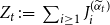 $Z_t\,:\!=\,\sum _{i\ge 1} J^{(\widetilde {\alpha }_t)}_i$
and for
 $M\gt 0$
,
 $Z^M_{t}=\sum _{i=1}^M J^{(\widetilde {\alpha }_t)}_i$
. Let choose
 $M\,:\!=\,M(t)$
such that
 \begin{equation*}(1-\varepsilon ) w_t-\mathbb{E}(Z^M_{t})=\sum _{i\gt M}\frac {tp_i}{tp_i+w_t}-\varepsilon w_t\le -\frac {\varepsilon w_t}{2}.\end{equation*}
We get
 \begin{equation*}\mathbb{P}(Z_{t}\le (1-\varepsilon )w_t)\le \mathbb{P}(Z^M_{t}\le (1-\varepsilon )w_t)\le \mathbb{P}\left (Z^M_{t}-\mathbb{E}(Z^M_{t})\le -\frac {\varepsilon w_t}{2}\right ).\end{equation*}
Using Bernstein inequality, we get
 \begin{equation*}\mathbb{P}(Z^M_{t}\le (1-\varepsilon )w_t)\le \exp \left (\!-\frac {\frac {(\varepsilon w_t)^2}{8}}{w_t\sum _{i=1}^M\frac {tp_i}{(tp_i+w_t)^2}+\frac {\varepsilon w_t}{3}}\right )\le \exp \left (\!-\frac {\frac {(\varepsilon w_t)^2}{8}}{w_t\sum _{i=1}^\infty \frac {tp_i}{(tp_i+w_t)^2}+\frac {\varepsilon w_t}{3}}\right ).\end{equation*}
Using Lemma 4.1 (v) we obtain, for
 $\varepsilon \in (0,1)$
,
 \begin{equation} \mathbb{P}(Z^M_{t}\le (1-\varepsilon )w_t)\le \exp \left (\!-\frac {\frac {(\varepsilon w_t)^2}{8}}{4w_t+\frac {\varepsilon w_t}{3}}\right )\le \exp \left (\!-\frac {\varepsilon ^2 w_t}{40}\right ). \end{equation}
We deduce from the previous proposition the following left-tail inequality for
 $L_n$
.
Proposition 5.2.
For all
 $\varepsilon \in (0,1)$
,
 $n\geq 1$
and every distribution
 $(p_i)_{i\geq 1}$
we have:
 \begin{equation*} \mathbb{P}(L_n\le {(1-\varepsilon )^2}w_n)\leq 3\exp \left (\!-\frac {\varepsilon ^2(1-\varepsilon )}{40}w_{n}\right )\!. \end{equation*}
Proof. We have
 \begin{eqnarray*} \mathbb{P}(L_n\le (1-\varepsilon )^2 w_n) & \le & \mathbb{P}(N_{n(1-\varepsilon )}\ge n)+\mathbb{P}(L_n\le (1-\varepsilon )^2 w_n, N_{n(1-\varepsilon )}\le n)\\ & \le & \mathbb{P}(N_{n(1-\varepsilon )}\ge n)+\mathbb{P}(L_{N_{n(1-\varepsilon )}}\le (1-\varepsilon )^2 w_n). \end{eqnarray*}
Using that
 $(1-\varepsilon )^2 w_n \le w_{n(1-\varepsilon )}(1-\varepsilon )$
(Lemma 4.1 (iv)) and Proposition 5.1, we get
 \begin{align*}\mathbb{P}(L_{N_{n(1-\varepsilon )}}&\le (1-\varepsilon )^2 w_n)\le \mathbb{P}(L_{N_{n(1-\varepsilon )}} \le (1-\varepsilon ) w_{n(1-\varepsilon )})\\ &\le 2\exp \left(\!-\frac {\varepsilon ^2}{40}w_{n(1-\varepsilon )}\right) \le 2\exp \left (\!-\frac {\varepsilon ^2(1-\varepsilon )}{40}w_{n}\right )\!, \end{align*}
using again that
 $ w_{n(1-\varepsilon )}\ge (1-\varepsilon )w_n$
for the last inequality. Now, using that
 $w_n\le n$
, we get
 \begin{equation*}\mathbb{P}(N_{n(1-\varepsilon )}\ge n)\le \exp \left(\!-\frac {n\varepsilon ^2}{40}\right)\le \exp \left (\!-\frac {w_n\varepsilon ^2}{40}\right )\!.\end{equation*}
Proof of (16): lower bound in Theorem 1.1. We have
 \begin{equation*}\mathbb{E}(L_n)\ge {(1-\varepsilon )^2}w_n \mathbb{P}(L_n\ge {(1-\varepsilon )^2}w_n).\end{equation*}
Thus Proposition 5.2 implies that, for all
 $\varepsilon \gt 0$
,
 \begin{equation*}\liminf _{n\to \infty } \frac {\mathbb{E}(L_n)}{w_n}\ge {(1-\varepsilon )^2}.\end{equation*}
6. Asymptotics of
$f_t$

Theorem 1.1 states that
 $L_n$
is asymptotically between
 $\frac {f_n}{2}$
and
 $f_n$
. In this section we try to determine the asymptotic behaviour of the deterministic sequence
 $f_n$
, with strategies that depend on
 $\mathbf p$
.
6.1 Preliminaries: a lower bound from a greedy algorithm
Neither Theorem 1.1 nor its proof gives a constructive way to find a long increasing subsequence. This section partially addresses the problem by presenting a simple greedy algorithm which, for a large class of distributions, produces a long increasing subsequence of the right asymptotic order of magnitude. Besides, this will provide estimates which will be used in the proofs of Propositions 1.1 and 1.2.
In order to explain the construction, let us first assume that
 $(p_i)_{i\ge 1}$
is non-increasing. Fix
 $n\ge 1$
and consider the increasing subsequence
 $(E_1,E_2,\ldots , E_{R_n})$
defined as follows:
-
•
$E_1$
is the first appearance of
$1$
in the sequence
$(X_k)_{k\ge 1}$
, namely,
$ E_1=\min \left \{k\geq 1; X_k=1\right \}$
. -
•
$E_2$
is the first appearance of
$2$
after
$E_1$
, namely,
$ E_2=\min \left \{k\geq E_1; X_k=2\right \}$
. -
•
$\ldots$
and so on for any
$i\ge 1$
.


Let
 $R_n$
be the largest index such that
 $E_{R_{n}}\le n$
. The sequence
 $(X_{E_1},X_{E_2},\ldots , X_{E_{R_n}})=(1,2,\ldots ,R_n)$
is thus an increasing subsequence of
 $(X_1,\ldots , X_n)$
. It is clear that
 $E_i-E_{i-1}$
is a geometric random variable with mean
 $1/p_i$
, so we expect that the length
 $R_n$
of the above subsequence satisfies
 $R_n \approx r_n$
whereFootnote
2
 \begin{equation*} r_n=\sup \left\{r\geq 1, \sum _{i=1}^{r}\frac {1}{p_i}\le n\right\}\!. \end{equation*}
This construction looks good if
 $\mathbf{p}$
is non-increasing but may give a very poor result in the case of a general
 $\mathbf{p}$
(imagine if
 $p_1$
is very small, or even zero). It is very easy to fix this by reordering the
 $p_i$
’s and this is the purpose of the general construction that we give now:
-
(1) For
$i\geq 1$
, let
$p^{\downarrow }_i$
be the
$i$
-th greatest element of the sequence
$\mathbf{p}$
(with multiplicity). In other words
$\mathbf{p}^{\downarrow }\,:\!=\,(p^{\downarrow }_i)_{i\ge 1}$
is the non-increasing rearrangement of the sequence
$\mathbf{p}$
. -
(2) For
$n\geq 1$
let
$r_n$
be uniquely defined by(19)
\begin{equation} r_n=\sup \Big\{r\geq 1, \sum _{i=1}^{r}\frac {1}{p^{\downarrow }_i}\le n\Big\}. \end{equation}
-
(3) Let
$i^{(n)}_1\lt i^{(n)}_2\lt \ldots \lt i^{(n)}_{r_n}$
be such that
\begin{equation*} \left \{p_{i^{(n)}_1},p_{i^{(n)}_2},\ldots , p_{i^{(n)}_{r_n}}\right \}= \left \{p^{\downarrow }_{1},p^{\downarrow }_{2},\ldots , p^{\downarrow }_{r_n}\right \}\!. \end{equation*}
-
(4) Then apply the construction of the non-increasing case:
-
•
$E_1$
is the first appearance of
$i^{(n)}_1$
in the sequence
$(X_k)_{k\ge 1}$
, namely,
$ E_1=\min \left \{k\geq 1;\, X_k=i^{(n)}_1\right \}$
. -
•
$E_2$
is the first appearance of
$i^{(n)}_2$
after
$E_1$
, namely,
$ E_2=\min \left \{k\geq E_1;\, X_k=i^{(n)}_2\right \}$
. -
•
$\ldots$
and so on for any
$i\le r_n$
.
-
-
(5) Finally return
$(X_{E_1},\ldots ,X_{E_{ R_n}})$
where
$R_n$
is the largest index such that we have that
$E_{R_{n}}\le n$
(note that by construction
$R_n\le r_n$
).


This algorithm returns an increasing subsequence of
 $(X_1,\ldots ,X_n)$
of length
 $R_n$
, implying in particular that
 $L_n\ge R_n$
. Observe that this algorithm is greedy for fixed
 $n$
but requires to know
 $n$
in advance in order to determine
 $i^{(n)}_1,i^{(n)}_2,\ldots$
. In particular the outputs of the algorithm for successive integers
 $n,n+1$
may differ significantly and the sequence
 $(R_n)_{n\ge 1}$
is not in general nondecreasing. Using this strategy, we obtain the following lower bound for
 $L_n$
.
Proposition 6.1.
For every distribution
 $\mathbf{p}$
, we have
 \begin{equation*}\liminf _n \frac {L_n}{r_n}\ge 1\qquad \mbox{a.s.}\end{equation*}
where
 $(r_n)_{n \ge 1}$
is given by(19).
Proof.
Let
 $\lambda \in (0,1)$
and
 $n\in \mathbb{N}$
. With the notation introduced above, observe that
 $R_n\lt \lfloor \lambda r_n\rfloor$
if and only if
 $E_{\lfloor \lambda r_n\rfloor }\gt n$
. Since
 $L_n\ge R_n$
, this yields
 \begin{equation*}\mathbb{P}(L_n\lt \lfloor \lambda r_n\rfloor )\le \mathbb{P}(R_n\lt \lfloor \lambda r_n\rfloor )=\mathbb{P}(E_{\lfloor \lambda r_n\rfloor }\gt n).\end{equation*}
Recalling that
 $E_{\lfloor \lambda r_n\rfloor }$
is the sum of
 $\lfloor \lambda r_n\rfloor$
independent geometric variables with respective parameters
 $(p^{\downarrow }_i)_{i\le \lfloor \lambda r_n\rfloor }$
, we get
 \begin{eqnarray*} \mathbb{P}(L_n\lt \lfloor \lambda r_n\rfloor ) & {\le } &\mathbb{P}\left (E_{\lfloor \lambda r_n\rfloor }-\sum _{i=1}^{\lfloor \lambda r_n\rfloor }\frac {1}{p^{\downarrow }_i} \gt n-\sum _{i=1}^{\lfloor \lambda r_n\rfloor }\frac {1}{p^{\downarrow }_i}\right )\\ & \leq &\mathbb{P}\left (E_{\lfloor \lambda r_n\rfloor }-\mathbb{E}[E_{\lfloor \lambda r_n\rfloor }] \gt \sum _{i=1}^{r_n} \frac {1}{p^{\downarrow }_i} -\sum _{i=1}^{\lfloor \lambda r_n\rfloor }\frac {1}{p^{\downarrow }_i}\right )\qquad \left(\text{using }\sum _{i=1}^{r_n}1/p^{\downarrow }_i\leq n\right)\\ & \le & \mathbb{P}\left (E_{\lfloor \lambda r_n\rfloor }-\mathbb{E}[E_{\lfloor \lambda r_n\rfloor }]\gt \sum _{i={\lfloor \lambda r_n\rfloor }+1}^{r_n}\frac {1}{p^{\downarrow }_i}\right )\\ & \le & \frac {\mbox{Var}(E_{\lfloor \lambda r_n\rfloor })}{ \left (\sum _{i={\lfloor \lambda r_n\rfloor }+1}^{r_n}\frac {1}{p^{\downarrow }_i}\right )^2}\\ & \le & \frac {\sum _{i=1}^{\lfloor \lambda r_n\rfloor }\frac {1}{p_i^{\downarrow ^2}}}{ \left (r_n(1-\lambda )\frac {1}{p^{\downarrow }_{\lfloor \lambda r_n\rfloor }}\right )^2} \le \frac {\lambda }{(1-\lambda )^2 r_n}. \end{eqnarray*}
Let us note that
 $(r_n)_{n \ge 1}$
is a non-decreasing integer sequence which tends to infinity and such that
 $r_{n+1}-r_{n}\le 1$
. Considering
 $(r_{m_n})_{n\ge 1}$
such that
 $r_{m_n}=n^2$
, the Borel-Cantelli Lemma yields that
 $L_{m_n}\ge \lfloor \lambda r_{m_n}\rfloor$
a.s. for
 $n$
large enough. Using the same trick as in Section 2, we easily deduce
 \begin{equation*}\liminf _m \frac {L_{m}}{r_{m}}\ge 1\qquad \mbox{a.s.}\end{equation*}
6.2 Bounds for
$f_t$

We have proved that,
 \begin{equation*}\liminf _n \frac {L_n}{r_n}\ge 1 \qquad \mbox{ and } \qquad \limsup _n \frac {L_n}{f_n}\le 1 \qquad \mbox{a.s.}\end{equation*}
So it is natural to try to find bounds on these two quantities for various distributions
 $\mathbf{p}$
.
Lemma 6.2.
Assume that
 $\textbf {p}$
is eventually non-increasing. Let
 $p:[0,\infty )\rightarrow (0,\infty )$
be an eventually non-increasing continuous function such that
 $p(n)=p_n$
for
 $n\in \mathbb{N}$
and let
 $\,\bar {\!F}(x)=\int _{x}^\infty p(u)du$
. Then, for
 $t$
large enough, there exist unique
 $\mu _t\gt 0$
and
 $\nu _t\gt 0$
such that
 \begin{equation} \frac {\mu _t}{p(\mu _t)}=t \qquad \mbox{ and } \qquad \frac {\nu _t^2}{\,\bar {\!F}(\nu _t)}=t. \end{equation}
Moreover, for
 $n$
large enough, we have
 \begin{equation} \lfloor \mu _n\rfloor \le r_n \text{ and } f_n \le {4}\nu _n. \end{equation}
Proof.
Using the fact that
 $p$
is eventually non-increasing, note that, for
 $x$
sufficiently large,
 \begin{equation*}\sum _{n\ge x+1} p_n\le \,\bar {\!F}(x)\le \sum _{n\gt x-1} p_n\le 1,\end{equation*}
so in particular
 $\,\bar {\!F}(x)$
is finite and bounded on
 $[0,\infty )$
. Moreover, for
 $t$
large enough
 $\mu _t$
and
 $\nu _t$
are well defined since the functions
 $x\mapsto \frac {x}{p(x)}$
and
 $x\mapsto \frac {x^2}{\,\bar {\!F}(x)}$
are both continuous, eventually increasing and tend to infinity. Note also that we necessarily have
 $\lim _{t\to \infty } \mu _t=\lim _{t\to \infty } \nu _t=\infty$
. We first prove the first inequality in (21). Since
 $\mathbf{p}$
is eventually non-increasing and
 $\mu _n$
tends to infinity, we get, for
 $n$
large enough,
 $p(\mu _n)\le p_i$
for all
 $i\le \mu _n$
. Thus, we deduce
 \begin{equation*}\sum _{i=1}^{\lfloor \mu _n\rfloor }\frac {1}{p_i}\le \frac {\lfloor \mu _n\rfloor }{p(\mu _n)}\le \frac {\mu _n}{p(\mu _n)}= n.\end{equation*}
So by definition of
 $r_n$
, we get
 $r_n\ge \lfloor \mu _n\rfloor$
.
Let us prove the second inequality in (21). The function
 $\frac {\,\bar {\!F}(x)}{{x}}$
is continuous, decreasing on
 $(0,\infty )$
from infinity to 0. Let
 $q$
be its inverse function, i.e., for all
 $a\gt 0$
,
 $\frac {\,\bar {\!F}(q(a))}{{q(a)}}=a$
. Note that
 $q$
is also decreasing and
 $\lim _{a\to 0^+}q(a)=\infty$
. Let
 $a_0$
such that
 $p$
is non-increasing on
 $[q(a_0),\infty )$
. Then, for
 $a\le a_0$
, we have
 \begin{align*} \sum _{i\geq 0}\frac {p_i}{p_i+a}\le \sum _{i\leq q(a)+1}\frac {p_i}{p_i+a}+ \sum _{i\gt q(a)+1}\frac {p_i}{p_i+a} &\leq q(a)+1+\sum _{i\gt q(a)+1}\frac {p_i}{a}\\ \ & \le \ q(a)+1+\frac {\,\bar {\!F}(q(a))}{a}=2q(a)+1. \end{align*}
Thus
 \begin{equation*}f_n \le \inf _{a\leq a_0}\left \{an+2q(a)+1\right \}.\end{equation*}
Taking
 $a=\nu _n/n$
, we have, for
 $n$
large enough,
 $a\le a_0$
since
 $\nu _n\le \sqrt {n ||\,\bar {\!F}||_\infty }$
. Thus, we obtain
 \begin{equation*} f_n \le \nu _n+2q(\nu _n/n)+1. \end{equation*}
By definition of
 $\nu _n$
we have that
 $\nu _n/n=\,\bar {\!F}(\nu _n)/\nu _n$
, so we get
 \begin{equation*}q(\nu _n/n)=q(\,\bar {\!F}(\nu _n)/\nu _n)=\nu _n\end{equation*}
and so, for
 $n$
large enough,
 \begin{equation*}f_n\le 3 \nu _n+1\le 4\nu _n.\end{equation*}
We now show that for light-tailed distributions
 $r_n$
and
 $f_n$
are of the same order, implying that our lower and upper bounds for
 $L_n$
are also of the same order. The proposition below applies for example for the geometric and Poisson distributions.
Proposition 6.3 (Asymptotics for sub-exponential distributions). Assume that
 $\limsup _i p_{i+1}/p_i\lt 1$
. Then, when
 $n\to +\infty$
,
 \begin{equation*} {f_n\sim w_n}\sim r_n\sim \mu _n. \end{equation*}
(For convenience we recall that
 ${f_n,w_n},r_n,\mu _n$
are respectively defined in (
1
), (
2
), (
19
), (
20
).)
Note that Proposition 6.3 combined with Theorem 1.1 implies that
 $\frac {L_n}{f_n}\to 1$
for all sub-exponential distributions.
Proof.
First, combining Theorem 1.1 with Proposition 6.1, we get
 $\liminf _n \frac {f_n}{r_n}\geq 1$
. Moreover, with Lemma 6.2, we know that
 $\liminf _n \frac {f_n}{\mu _n}\ge 1$
(the assumption
 $\limsup _i p_{i+1}/p_i\lt 1$
ensures that
 $(p_i)_{i\ge 1}$
is eventually non-increasing).
Let us show that
 $\limsup _n \frac {f_n}{\mu _n}\le 1$
. Let
 $\varepsilon \gt 0$
and
 $n\in \mathbb{N}$
. We write (recall that
 $g_n$
was defined in (11))
 \begin{align*} g_n(\varepsilon \frac {\mu _n}{n})&=\varepsilon \mu _n+\sum _{i=1}^{\lfloor \mu _n\rfloor }\frac {p_i}{p_i+\varepsilon \frac {\mu _n}{n}}+\sum _{i=\lfloor \mu _n\rfloor +1}^{+\infty }\frac {p_i}{p_i+\varepsilon \frac {\mu _n}{n}}\\ &\le \varepsilon \mu _n +\sum _{i=1}^{\lfloor \mu _n\rfloor }1+\sum _{i=\lfloor \mu _n\rfloor +1}^{+\infty }\frac {n}{\varepsilon \mu _n}p_i\\ &\le \varepsilon \mu _n+\mu _n+\frac {n}{\varepsilon \mu _n}\sum _{i\gt \mu _n}p_i. \end{align*}
Now, since
 $\limsup _i \frac {p_{i+1}}{p_i}\lt 1$
, there exists
 $0\lt \lambda \lt 1$
and
 $j\in \mathbb{N}$
such that for all
 $i\geq j$
and
 $k\geq 0$
,
 $p_{i+k}\le p_i\lambda ^k$
. Thus for all
 $i\in \mathbb{N}$
 \begin{equation*} \sum _{k\gt i}p_k\le p_i\sum _{k=0}^{+\infty }\lambda ^k=p_i\frac {1}{1-\lambda }. \end{equation*}
It yields that
 \begin{equation*} f_n\le g_n(\varepsilon \frac {\mu _n}{n})\le (1+\varepsilon )\mu _n+ \frac {n}{\varepsilon \mu _n}p(\mu _n)\frac {1}{1-\lambda }. \end{equation*}
Since
 $\frac {np(\mu _n)}{\mu _n}=1$
we finally have
 \begin{equation*} f_n\le (1+\varepsilon )\mu _n+\frac {1}{(1-\lambda )\varepsilon }, \end{equation*}
which implies
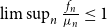 $ \limsup _n \frac {f_n}{\mu _n}\le 1$
(recall that
 $\mu _n\to +\infty$
). Now, according to Lemma 6.2, for
 $n$
large enough
 $\lfloor \mu _n\rfloor \le r_n$
so
 \begin{equation*} \limsup _n \frac {f_n}{r_n}\le \limsup _n \frac {f_n}{\mu _n}\le 1, \end{equation*}
thus
 \begin{equation*} \lim _{n\to +\infty }\frac {f_n}{r_n}=\lim _{n\to +\infty }\frac {f_n}{\mu _n}=1 \end{equation*}
i.e.
 $f_n\sim \mu _n\sim r_n$
. Since,
 $w_n\le f_n$
, it remains to find a lower bound of
 $w_n$
of the same order. Let
 $\varepsilon \gt 0$
and let us prove that, for
 $n$
large enough,
 $w_n\ge \mu _n(1-\varepsilon )\,:\!=\,t_n$
. For
 $n\ge 0$
, put
 \begin{equation*}h_n(x)\,:\!=\,\sum _{i\ge 1} \frac {np_i}{np_i+x}\end{equation*}
so that
 $h_n(w_n)=w_n$
. We show that
 $h_n(t_n)\ge t_n$
. Since
 $h_n$
is a non-increasing function, this would imply that
 $w_n\ge t_n$
and conclude the proof. Let
 $\eta \gt 0$
such that
 $(1-\eta )/(1+\eta )=(1-\varepsilon )$
and let
 \begin{equation*}I_n\,:\!=\,\{i\ge 1, \frac {t_n}{np_i}\le \eta \}.\end{equation*}
We have
 \begin{equation*}h_n(t_n)\ge \sum _{i\in I_n} \frac {1}{1+\frac {t_n}{np_i}}\ge |I_n|\frac {1}{1+\eta }.\end{equation*}
We need now to find a lower bound on the cardinal of
 $I_n$
. We claim, that for
 $n$
large enough,
 \begin{equation*}|I_n|\ge (1-\eta )\mu _n.\end{equation*}
Indeed recalling that
 $p(\mu _n)=\mu _n/n$
, we have
 \begin{equation*}i\in I_n \Longleftrightarrow p_i\ge \frac {t_n}{\eta n} \Longleftrightarrow p(\mu _n)\le \frac {\eta }{(1-\varepsilon )}p_i.\end{equation*}
Using that
 $\mathbf{p}$
is sub-exponential, we have, for
 $n$
large enough and
 $i\le (1-\eta )\mu _n$
,
 \begin{equation*}p(\mu _n)\le \lambda ^{\eta \mu _n} p((1-\eta )\mu _n)\le \lambda ^{\eta \mu _n} p_i\end{equation*}
and so
 $i\in I_n$
if
 $n$
is large enough such that
 $\lambda ^{\eta \mu _n}\le \eta /(1-\varepsilon )$
. Hence, we get
 \begin{equation*}h_n(t_n)\ge \frac {1-\eta }{1+\eta }\mu _n=t_n.\end{equation*}
We now give a lemma comparing
 $(\mu _t)_{t\gt 0}$
and
 $(\nu _t)_{t\gt 0}$
for heavy tailed distribution regularly varying with index strictly larger than
 $1$
. This lemma will be useful for the proof of Proposition 1.2 below.
Lemma 6.4.
If
 $p_i= \ell (i)i^{-\gamma }$
with
 $\gamma \gt 1$
and
 $\ell$
slowly varying and
 $\mathbf{p}$
is eventually non-increasing, then, for all
 $c\gt 1$
, for
 $t$
large enough
 $ \nu _t \le \mu _{ct/(\gamma -1)}$
.
Proof.
If
 $p_i= \ell (i)i^{-\gamma }$
, then
 $\,\bar {\!F}(i){=\int _{i}^\infty p(u)du \sim } \sum _{j\gt i}p_j\sim \frac {1}{\gamma -1}\ell (i)i^{-\gamma +1}$
(see [Reference Feller9], Section VIII.9, Theorem 1). In particular, for any
 $c\gt 1$
and
 $x$
large enough,
 \begin{equation*}\,\bar {\!F}(x)\le \frac {c}{\gamma -1}x p(x).\end{equation*}
Thus, for
 $t$
large enough
 \begin{equation*}\nu _t^2=t\,\bar {\!F}(\nu _t)\le t\frac {c }{\gamma -1}\nu _t p(\nu _t)\end{equation*}
and so
 \begin{equation*}\frac { \nu _t}{p( \nu _t )}\le \frac {tc }{\gamma -1}= \frac { \mu _{tc/(\gamma -1)} }{p( \mu _{tc/(\gamma -1)})}.\end{equation*}
We use again that the function
 $x\rightarrow x/p(x)$
is increasing to conclude.
6.3 Some explicit estimates
Recall that
 $\mu _n$
was defined in (20) as the solution of
 $\frac {\mu _n}{p(\mu _n)}=n$
. The combination of Lemma 6.2, Proposition 6.3 and Lemma 6.4 allow to translate bounds for
 $\mu _n$
into bounds for
 $f_n$
, for various distributions. The purpose of the next lemma is therefore to estimate
 $\mu _n$
in several cases.
Lemma 6.5.
-
• If
$\textbf {p}$
is a geometric distribution
$p_i\,:\!=\,p (1-p)^{i-1}$
, then
(22)
\begin{equation} \mu _n\sim \frac {\log n}{|\log (1-p)|}. \end{equation}
-
• If
$\textbf {p}$
is a Poisson distribution
$p_i\,:\!=\,\frac {e^{-\lambda }\lambda ^i }{i!}$
, then
(23)
\begin{equation} \mu _n\sim \frac {\log n}{|\log \log n|}. \end{equation}
-
• If
$\textbf {p}$
is eventually non-increasing and
$p_i\sim c i^{-\beta }(\log i)^\gamma$
,
$\beta \gt 1$
,
$\gamma \in \mathbb{R}$
, then
\begin{equation*} \mu _n\sim \left ( c n\left (\frac {\log n}{(1+\beta )}\right )^\gamma \right )^{1/(1+\beta )}. \end{equation*}


Proof.
Recall that
 $p:[0,\infty )\rightarrow (0,\infty )$
is an eventually non-increasing continuous function such that
 $p(i)=p_i$
for
 ${i}\in \mathbb{N}$
and, as noted previously,
 $\lim _{n\to +\infty }\mu _n =+\infty$
.
-
• Assume that
$p_i=p(1-p)^{i-1}$
and define the function
$p$
for
$x\ge 1$
by
$p(x)=p(1-p)^{x-1}$
. ThenThus we have
\begin{equation*} \frac {\mu _n}{n}=p(\mu _n)=p(1-p)^{\mu _n-1}. \end{equation*}
Now, since
\begin{equation*} \log \mu _n - \mu _n\log (1-p) =\log n+\log \left (\frac {p}{1-p}\right ). \end{equation*}
$\log {\mu _n}=o(\mu _n)$
, we get
$\mu _n|\log (1-p)|\sim \log n$
, hence (22).
-
• Consider now the distribution
$p_i=\frac {e^{-\lambda }\lambda ^i}{i!}$
and for
$x\ge 1$
set
$p(x)= e^{-\lambda }\frac {\lambda ^x}{\Gamma (x+1)}$
. The function
$p$
is increasing on
$[1,x_\lambda ]$
and decreasing on
$[x_\lambda ,+\infty )$
for some
$x_\lambda \gt 1$
. Since
$\mu _n\to +\infty$
, there exists
$n(\lambda )\in \mathbb{N}$
such that for all
$n\geq n(\lambda )$
,
$\mu _n\geq x_\lambda$
. For such
$n$
,Now, since
\begin{equation*} p(\mu _n)=\frac {\mu _n}{n}=\frac {e^{-\lambda }\lambda ^{\mu _n}}{\Gamma (\mu _n+1)}. \end{equation*}
$\Gamma (\mu _n+1)=\mu _n\Gamma (\mu _n)$
we getThanks to the Stirling formula we can write:
\begin{equation*} \mu _n^2\frac {\Gamma (\mu _n)}{\lambda ^{\mu _n}}=\frac {n}{e^\lambda }. \end{equation*}
Now by taking the logarithm and using that
\begin{equation*} \mu _n^2\times \left (\frac {\mu _n}{\lambda e} \right )^{\mu _n}\sqrt {2\pi \mu _n}\sim \frac {n}{e^\lambda }. \end{equation*}
$\log \mu _n$
and
$ \mu _n$
are negligible compared to
$\mu _n \log \mu _n$
, we get
$ \mu _n\log (\mu _n)\sim \log (n)$
. Applying the logarithm a last time, we then obtain
$\log (\mu _n)\sim \log (\log (n))$
, hence (23).
-
• Let
$\beta \gt 1$
,
$\gamma \in \mathbb{R}$
and assume that
$p_i\sim c(\log i)^\gamma i^{-\beta }$
, so
$p(\mu _n)\sim c(\log \mu _n)^\gamma \mu _n^{-\beta }$
for
$n$
large enough. We getTaking the logarithm, we get
\begin{equation*}n=\frac {\mu _n}{p(\mu _n)}\sim \frac {\mu _n^{1+\beta }}{c(\log \mu _n)^\gamma }.\end{equation*}
Plugging this in the previous equation, we get
\begin{equation*}\log n \sim (1+\beta ) \log \mu _n.\end{equation*}
which yields the result.
\begin{equation*}\mu _n^{1+\beta }\sim c n\left (\frac {\log n}{(1+\beta )}\right )^\gamma .\end{equation*}


Proof of Proposition 1.1. Using Theorem 1.1, we know that
 \begin{equation*}\liminf _n \frac {L_n}{w_n}\ge 1 \qquad \limsup _n \frac {L_n}{f_n}\le 1 \qquad a.s.\end{equation*}
Moreover, if
 $\mathbf{p}$
is a geometric or a Poisson distribution, thanks to Proposition 6.3, we know that
 $f_n\sim w_n \sim \mu _n$
. Then we estimate
 $\mu _n$
using Lemma 6.5 in order to deduce Proposition 1.1.
Proof of Proposition 1.2. Recall that
 $\mu _n$
and
 $\nu _n$
are defined by (20). Combining Proposition 6.1 and Lemma 6.2, we obtain
 \begin{equation} \liminf _n \frac {L_n}{\mu _n}= \liminf _n \frac {L_n}{r_n}\times \frac {r_n}{\mu _n} \geq 1 \times 1 \gt 0. \end{equation}
Besides, combining Theorem 1.1 and Lemma 6.2 yields
 \begin{equation} \limsup _n \frac {L_n}{\nu _n}= \limsup _n \frac {L_n}{f_n} \times \frac {f_n}{\nu _n} \leq 1 \times {4} \lt +\infty . \end{equation}
In the case
 $p_i\sim c (\log i)^\gamma i^{-\beta }$
with
 $\beta \gt 1$
, we deduce (i) in Proposition 1.2 using the asymptotic for
 $\mu _n$
computed in Lemma 6.5 and the upper bound for
 $\nu _n$
given in Lemma 6.4.
Let us now consider the case (ii) of Proposition 1.2, namely
 $p_i\sim c (\log i)^\gamma i^{-1}$
with
 $\gamma \lt -1$
. Then, we have, for some
 $c_1\gt 0$
,
 \begin{equation*} \,\bar {\!F}(x){\sim } \sum _{i\gt x} p_i \sim c_1(\log x)^{\gamma +1}.\end{equation*}
As
 $\frac {\nu _n^2}{\,\bar {\!F}(\nu _n)}=n$
this implies that
 \begin{equation*}\nu _n\sim c_2\sqrt {n(\log n)^{\gamma +1}}\end{equation*}
for some
 $c_2 \gt 0$
. This asymptotic combined with (25) yields the upper bound
 \begin{equation*}\limsup _n \frac {L_n}{\sqrt {n(\log n)^{\gamma +1}}}\lt \infty .\end{equation*}
An easy computation shows that
 $\mu _n\sim c_3{\sqrt {n(\log n)^{\gamma }}}$
, so we will not obtain the desired lower bound for
 $L_n$
just using that asymptotically
 $L_n\ge \mu _n$
. We should make here more precise computation to find a lower bound for
 $f_n$
(and so for
 $w_n$
).
Recall that
 $p(x)$
is eventually non-increasing and such that
 $p(i)=i$
for every positive integer
 $i$
. For
 $a$
close to
 $0$
, let
 $u(a)$
be such that
 $a=p(u(a))$
. Thus
 \begin{equation*} a \stackrel {a\to 0}{\sim } c (\log u(a))^\gamma u(a)^{-1} \end{equation*}
which implies
 \begin{equation*} u(a)\stackrel {a\to 0}{\sim } c |\log a|^\gamma a^{-1}. \end{equation*}
Using that
 $\mathbf{p}$
is eventually non-increasing, we have, for
 $a$
close to
 $0$
,
 $p_i\le a$
if
 $i\ge u(a)$
. So we get
 \begin{equation*}\sum _{i=1}^\infty \frac {p_i}{p_i+a} \ge \sum _{i\ge u(a)} \frac {p_i}{a+a} \sim \frac {\,\bar {\!F}(u(a))}{2a} \sim \frac {c_1|\log a|^{\gamma +1}}{2a}.\end{equation*}
Hence, we get, for
 $n$
large enough
 \begin{equation*} f_n= \inf _{a\geq 0}\left \{ an+\sum _{i\geq 0}\frac {p_i}{p_i+a}\right \}\ge \inf _{a\geq 0}\left \{ an+\frac {c_1|\log a|^{\gamma +1}}{4a }\right \}\sim c_3\sqrt {n(\log n)^{\gamma +1}}. \end{equation*}
Using Theorem 1.1 and that
 $w_n\ge f_n/2$
, this yields the expected lower bound:
 \begin{equation*}\liminf _n \frac {L_n}{\sqrt {n(\log n)^{\gamma +1}}}\gt 0.\end{equation*}
Remark 6.1. In the case
 $p_i\sim c (\log i)^\gamma i^{-1}$
with
 $\gamma \lt -1$
, we can also compute the order of
 $r_n$
. Indeed, up to constant,
 ${\sum _{i\le k}} \frac {1}{p_i}\sim c{\sum _{i\le k}} i (\log i)^{-\gamma } \sim c_4k^2 (\log k)^{-\gamma }$
And so
 $r_n$
is such that
 $c_4r_n^2 (\log r_n)^{-\gamma } \sim n$
which yields
 $r_n\sim c_5\sqrt {n (\log n)^\gamma }$
. Hence, we see that
 $L_n\gg r_n$
which shows that in this case, the greedy algorithm described in Section 6.1 does not give a subsequence of the right order.
7. Case of a generic distribution: proof of Theorem 1.2
We explain in this section how Theorem 1.1, dealing with discrete distributions on integers, can in fact be extended to any discrete distribution, even if its support cannot be enumerated in increasing order, as in the cases of
 $\mathbb{Z}$
or
 $\mathbb{Q}$
. Let us first observe that the proof of
 $L_n/\mathbb{E}(L_n)\to 1$
(i.e. (3)) is valid for any distribution
 $\rho$
. Therefore, in order to extend the Theorem 1.1 to arbitrary distributions we just need to control
 $\mathbb{E}(L_n)$
.
Proof of Theorem 1.2. We begin by proving item (i) in Theorem 1.2. Let
 $\rho$
be a discrete distribution on a countable set
 $S\,:\!=\,\{i_1,i_2,\ldots \}$
. Let
 $(X_i)_{i\ge 1}$
be an i.i.d. sequence with law
 $\rho$
and for
 $M,n\ge 1$
, set
 \begin{equation*}D_n^M\,:\!=\,\{1\le i \le n, X_i\in \{i_1,\ldots ,i_M\}\}.\end{equation*}
We define
 $L_n^M\,:\!=\,L((X_i)_{i\in D_n^M})$
, the length of the longest increasing subsequence with values in
 $\{i_1,\ldots ,i_M\}$
. Since the set
 $\{i_1,\ldots ,i_M\}$
is finite, it can be enumerated in the increasing order and so we can apply Theorem 3.1 : if
 $N_t$
is a Poisson random variable with parameter
 $t$
independent of the sequence
 $(X_i)_{i\ge 1}$
, then, for any
 $\alpha \gt 0$
, we have the stochastic domination :
 \begin{equation*} L^M_{N_t} \leq \mathcal{H}^{(\alpha )}_t+ \sum _{j=1}^M I^{(\alpha )}_j, \end{equation*}
where
 $\mathcal{H}^{(\alpha )}_t$
is a Poisson random variable with parameter
 $\alpha t$
and
 $(I^{(\alpha )}_j)_{j \geq 1}$
is a sequence of independent random variables with
 $\mathrm{Bernoulli}\left (\frac {\rho (\{i_j\})}{\alpha +\rho (\{i_j\})}\right )$
distribution. Thus, for any
 $\alpha \gt 0$
 \begin{equation*} \mathbb{E}( L^M_{N_t} )\leq \alpha t + \sum _{j=1}^M \frac {\rho (\{i_j\})}{\alpha +\rho (\{i_j\})} \le \alpha t + \sum _{i\in S} \frac {\rho (\{i\})}{\alpha +\rho (\{i\})}. \end{equation*}
Optimizing over
 $\alpha$
, we get
 $\mathbb{E}( L^M_{N_t} )\le f_t$
and so, by monotone convergence,
 $\mathbb{E}( L_{N_t} )\le f_t$
. We conclude as in Section 5.1 that
 \begin{equation*}\limsup _n \frac {\mathbb{E}(L_n)}{f_n}\le 1.\end{equation*}
Regarding the lower bound, using again Theorem 3.1, we get the stochastic lower bound
 \begin{equation*} L_{N_t} \geq L^M_{N_t} \geq \min \Bigg(\mathcal{H}^{(\alpha )}_t, \sum _{j=1}^M J^{(\alpha )}_j\Bigg). \end{equation*}
Let
 $w_t$
the unique positive solution of the equation
 \begin{equation*} w_t=\sum _{i\in S} \frac {t\rho (\{i\})}{t\rho (\{i\})+w_t} \end{equation*}
and take
 $\widetilde {\alpha }_t=w_t/t$
. We get
 \begin{equation*} \mathbb{P}(L_{N_t}\lt (1-\varepsilon )w_t)\leq \mathbb{P}(\mathcal{H}^{(\widetilde {\alpha }_t)}_t\le (1-\varepsilon )w_t)+ \mathbb{P}(Z^M_{t}\le (1-\varepsilon )w_t), \end{equation*}
where
 $Z^M_{t}\,:\!=\,\sum _{i=1}^M J^{(\widetilde {\alpha }_t)}_i$
. One can check that (17) and (18) still hold in this case if
 $M$
is chosen large enough and thus imply that
 \begin{equation*} \mathbb{P}(L_{N_t}\lt (1-\varepsilon )w_t)\leq 2\exp \left (\!-\frac {\varepsilon ^2 w_t}{40}\right ), \end{equation*}
as obtained in Proposition 5.1 in the case of a distribution on the integers. We conclude, as in Section 5.2, that
 \begin{equation*}\liminf _n \frac {\mathbb{E}(L_n)}{w_n}\ge 1.\end{equation*}
Let us now prove item (ii) in Theorem 1.2. Let
 $\rho$
be a probability measure on
 $\mathbb{R}$
and write
 $\rho =\rho _1+\rho _2$
where
 $\rho _1$
is atomless and
 $\rho _2$
is purely discrete. Let
 $S$
be the (countable) support of
 $\rho _2$
. For
 $n\ge 1$
, define
 \begin{equation*}D^1_n\,:\!=\,\{i\le n, X_i\notin S\} \qquad \mbox{ and }\qquad D^2_n\,:\!=\,\{i\le n, X_i\in S\}\end{equation*}
and set
 $L_n^1\,:\!=\,L((X_i)_{i\in D^1_n})$
and
 $L_n^2\,:\!=\,L((X_i)_{i\in D^2_n})$
. Note that, for
 $k\in \{1,2\}$
,
 $|D^k_n|$
is a binomial random variable with parameters
 $(n,\rho _k(\mathbb{R}))$
. Moreover, since
 $\rho _1$
is atomless, conditionally on
 $|D^1_n|$
,
 $L_n^1$
has the law of
 $\mathcal{L}_{|D^1_n|}$
, the length of the longest increasing subsequence in a uniform permutation of size
 $|D^1_n|$
. Besides, we have
 \begin{equation*}L_n^1\le L_n\le L_n^1+L_n^2.\end{equation*}
On the one hand, using (i) of Theorem 1.2 and the fact that
 $f_n=o(\sqrt {n})$
for any discrete distribution, we get
 \begin{equation*}\lim _{n\to \infty } \frac {L_n^2}{\sqrt {n}}=0 \mbox{ a.s.}\end{equation*}
On the other hand, using the Veršik-Kerov’s theorem on uniform permutations [Reference Veršik and Kerov25], we obtain
 \begin{equation*}\lim _{n\to \infty } \frac {L_n^1}{2\sqrt {|D_n^1|}}=1 \mbox{ a.s.}\end{equation*}
as soon as
 $|D_n^1|$
converges to infinity almost surely. We conclude using the fact that, if
 $\rho _1(\mathbb{R})\gt 0$
, then
 $|D_n^1|\sim n\rho _1(\mathbb{R})$
almost surely.
Acknowledgements
Thank you to the reviewer who read the article very carefully and whose comments and suggestions helped to improve the presentation. All authors are supported by the project ANR LOUCCOUM.


 X1,…,Xn
 n=200
 pi≍i−2.2
 Ln=10

 X1,…,Xn
 n=200
 pi≍0.6i
 Ln=9
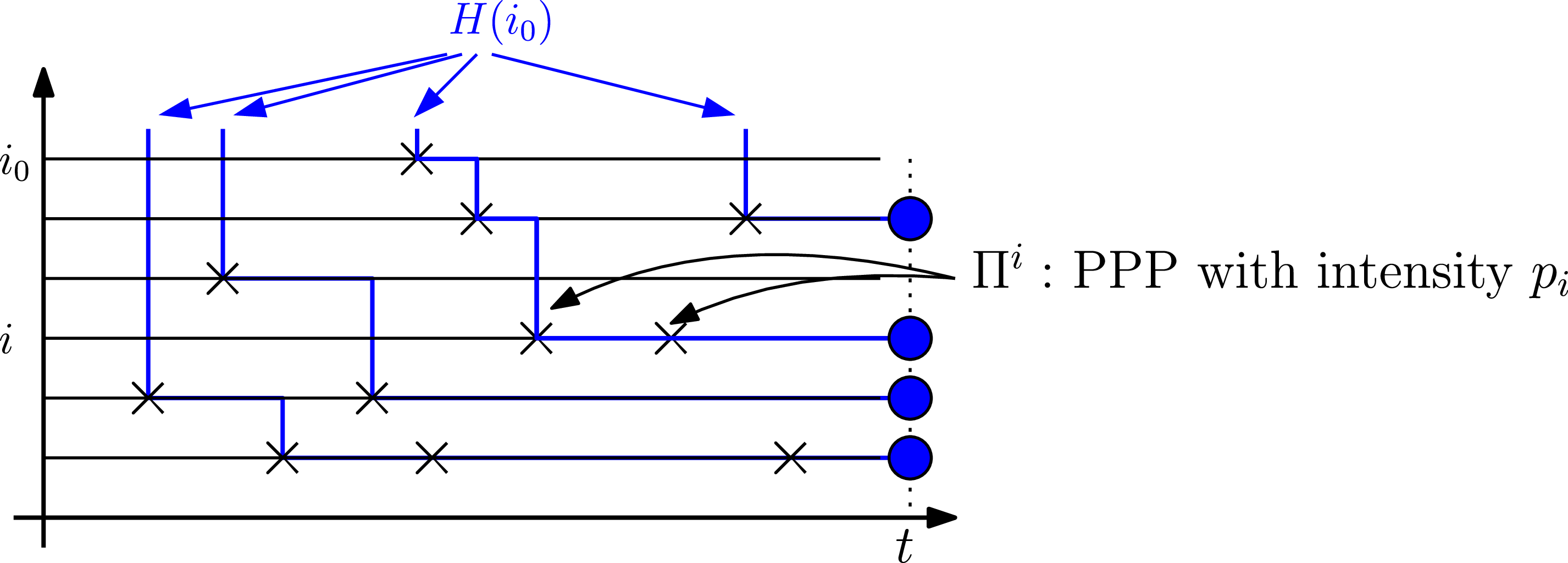
 Πt
 (H(i))i≥1
 L(Πt≤i0)=4=card(H(i0))
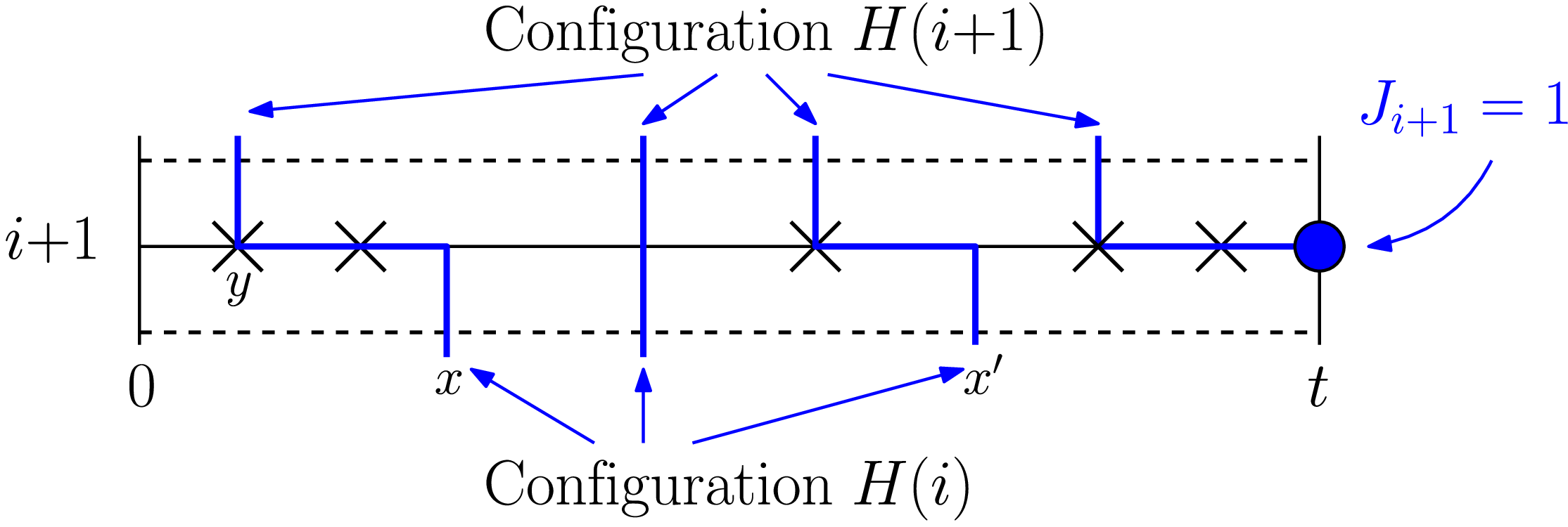
 H(i+1)
 H(i)
 Πi+1
 Πi+1
 ×
 Ji+1=1
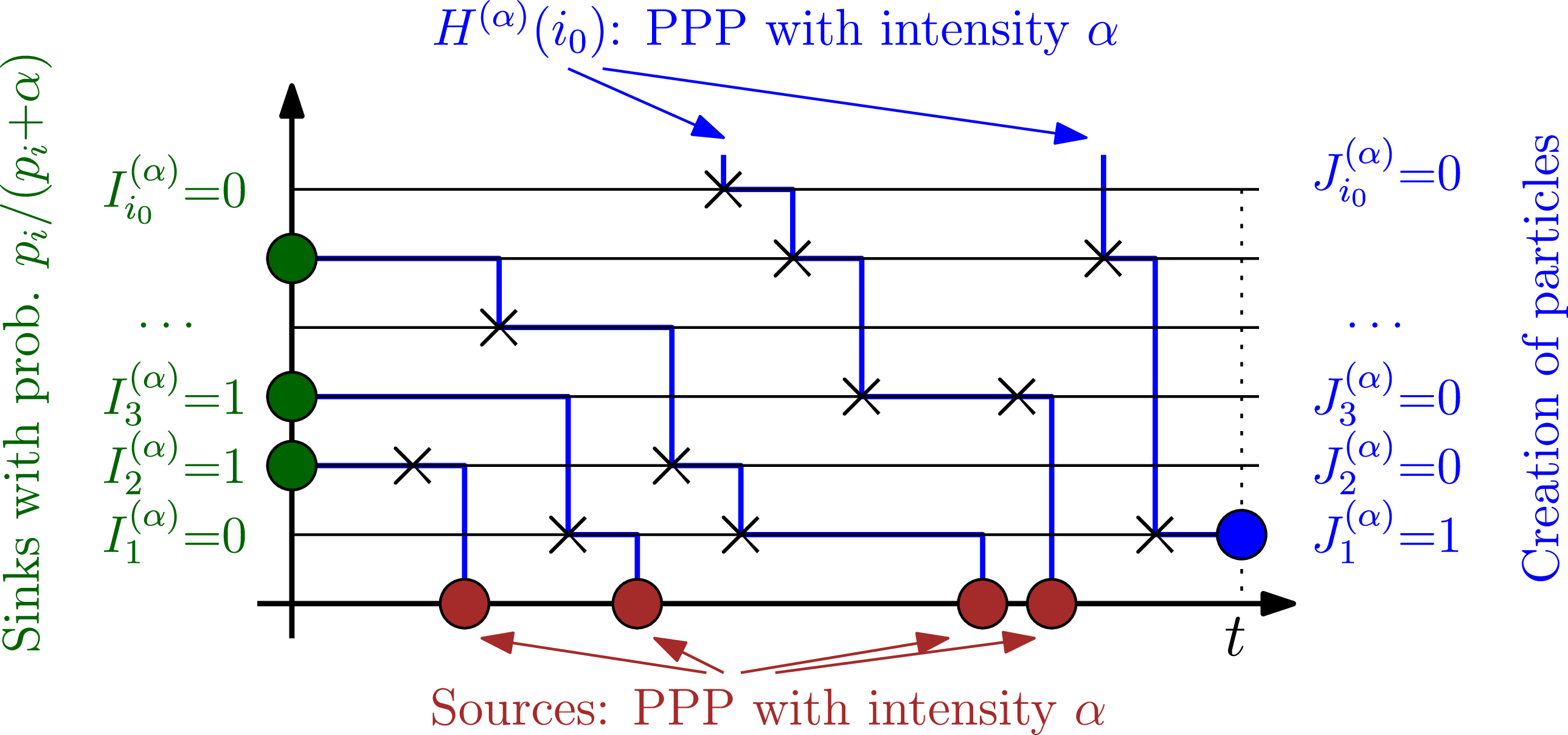
 Π
 I2(α)=I3(α)=I5(α)=1
 Ii(α)
 (H(α)(i))i≥1
 H(α)(i0)
 α

 (H(α)(i))i≥0
 pi≍i−1.2
 α=0.2
 n=100
 Π
 ∙
 α

 (H(α)(i))i≥0
 Π
 α=0.6
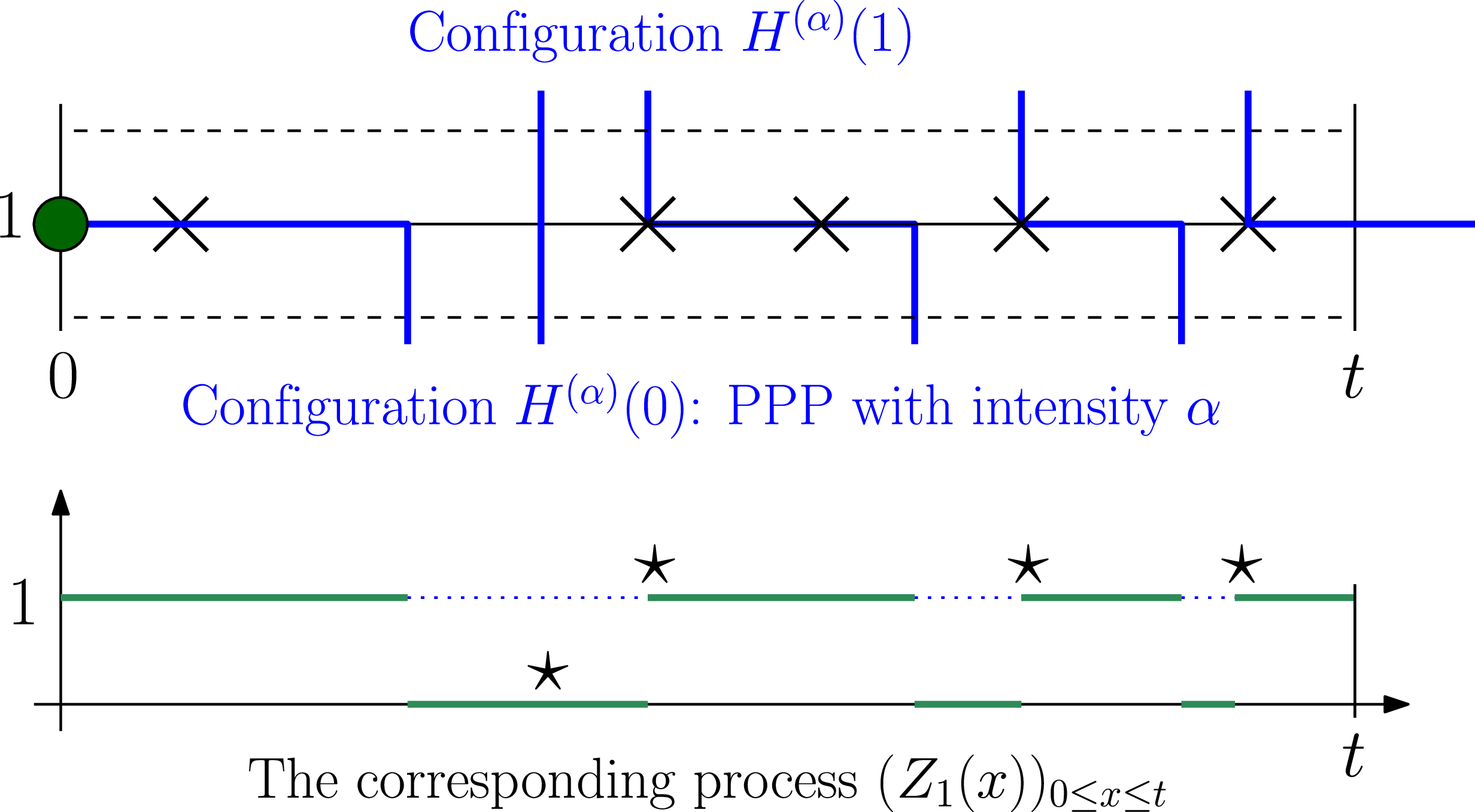
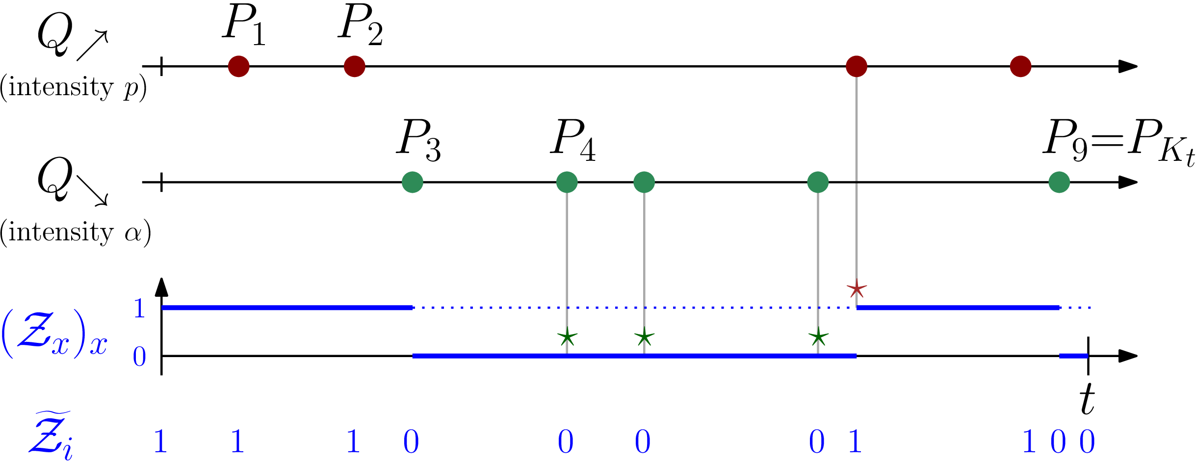
 Q=Q0∪Q1
 ⋆
 ⋆
 Q0
 ⋆
 Q1

 Open access

