1. Introduction
Mesoscale and submesoscale eddies (i.e. eddies with typical scales of the order of the Rossby deformation radius and below) are ubiquitous in the ocean (e.g. McWilliams Reference McWilliams1985; Munk et al. Reference Munk, Armi, Fischer and Zachariasen2000), and much effort has been dedicated to the analysis of such structures, especially with respect to their stability. Basically, two different types of vortex configurations have been considered since the early 1980s, namely columnar barotropic or vertically confined ones (the latter modelling surface-intensified eddies and subsurface lenses). Vortices of both types can be studied by means of laboratory experiments or numerical simulations and allow for analytical treatment under some simplifying assumptions. Mesoscale vortices at low Rossby numbers can be unstable with respect to the geostrophically balanced perturbations giving rise to classical barotropic and baroclinic instabilities, as proved by means of numerical linear stability analysis – often in two-layer models (Dewar & Killworth Reference Dewar and Killworth1995; Baey & Carton Reference Baey and Carton2002; Benilov Reference Benilov2003, Reference Benilov2004; Katsman et al. Reference Katsman, Van Der Vaart, Dijkstra and De Ruijet2003) – or by analytical stability arguments for specific radial profiles of the vorticity (Ripa Reference Ripa1992; Ford Reference Ford1994). Nonlinear saturation of such instabilities is well documented in the framework of quasi-geostrophic (Ikeda Reference Ikeda1981; Gent & McWilliams Reference Gent and McWilliams1986) or full two-layer rotating shallow water (RSW) models (Baey & Carton Reference Baey and Carton2002; Thivolle-Cazat, Sommeria & Galmiche Reference Thivolle-Cazat, Sommeria and Galmiche2005). It has been found that destabilization of barotropic isolated eddies concerns primarily the smaller ones (i.e. with high Burger numbers), while baroclinic instability switches on at low Burger numbers (and for baroclinic vortices). Both generally lead either to the formation of vortex tripoles, or to the vortex breakdown into dipoles.
Besides the geostrophic instabilities, the vortices can experience ageostrophic instabilities when their azimuthal velocity is sufficiently large. These instabilities are much less documented, except for the widely known centrifugal instability of columnar vortices. The first analysis of the centrifugal instability is due to Rayleigh (Reference Rayleigh1917), who found that the angular momentum in a revolving homogeneous fluid must decrease with the radius somewhere in the flow in order for instability to exist. Vortices in the ocean or the atmosphere are subject to stratification and background rotation, which modify this condition (Kloosterziel & van Heijst Reference Kloosterziel and van Heijst1991; Billant & Gallaire Reference Billant and Gallaire2005; Park & Billant Reference Park and Billant2013). The influence of stratification on the linear stability of vortices on the
 $f$
-plane (i.e. at constant Coriolis parameter) was investigated by Gent & McWilliams (Reference Gent and McWilliams1986), Smyth & McWilliams (Reference Smyth and McWilliams1998), Potylitsin & Peltier (Reference Potylitsin and Peltier1998) and Lazar, Stegner & Heifetz (Reference Lazar, Stegner and Heifetz2013b
), with a general result that the growth rate of the centrifugal instability is reduced when the stratification strengthens, but still remains higher than that of the barotropic or baroclinic instabilities. Studies of the impact of developing centrifugal instability upon intense vortices are relatively rare (Smyth & McWilliams Reference Smyth and McWilliams1998; Orlandi & Carnevale Reference Orlandi and Carnevale1999; Kloosterziel, Carnevale & Orlandi Reference Kloosterziel, Carnevale and Orlandi2007; Lazar et al.
Reference Lazar, Stegner, Caldeira, Dong, Didelle and Viboud2013a
). A detailed numerical investigation of the nonlinear saturation of this instability in a geophysical context has been reported only in Kloosterziel et al. (Reference Kloosterziel, Carnevale and Orlandi2007), to our knowledge, in the case of a continuously stratified, barotropic and strictly axisymmetric vortex on the
 $f$
-plane. The reasons for such sparseness in the literature, besides the fact that the importance of the centrifugal instability for geophysical flows has been fully realized only relatively recently, reside in the numerical cost of the simulations owing to the complexity of the flow resulting from the developing instability. It is well known that the centrifugal instability (as well as the inertial one, which is its analogue for the plane-parallel flows) exhibits the ultraviolet catastrophe (Smyth & Peltier Reference Smyth and Peltier1994; Smyth & McWilliams Reference Smyth and McWilliams1998), hence the necessity to resolve very fine scales.
Yet, the centrifugal instability does not need a fully three-dimensional flow to be realized, and manifests itself already in the two-layer rotating shallow water model, like the inertial one (e.g. Zeitlin Reference Zeitlin2008). Multi-layer RSW models are standard conceptual models in geophysical fluid dynamics (Pedlosky Reference Pedlosky1987; Vallis Reference Vallis2006). The technical advantages of these models – which retain, nevertheless, all pertinent features of the full ‘primitive’ equations – are that vertical structure is very coarse and easily controlled, which makes the linear stability analysis relatively simple. (The variations of stratification are difficult to include in the linear stability analysis of vortices in a continuously stratified fluid, where the strong assumptions of constant stratification and barotropicity are needed to make the mathematical problem separable. We are not aware of such results.) Besides, the model admits powerful high-resolution finite-volume numerical schemes (Bouchut & Zeitlin Reference Bouchut and Zeitlin2010) allowing for numerical simulations of nonlinear saturation of the instabilities for long evolution times and at a low computational cost (Bouchut, Ribstein & Zeitlin Reference Bouchut, Ribstein and Zeitlin2011). Because of these advantages, and following previous studies (Dewar & Killworth Reference Dewar and Killworth1995; Baey & Carton Reference Baey and Carton2002; Katsman et al. Reference Katsman, Van Der Vaart, Dijkstra and De Ruijet2003), we undertake below a detailed analysis of the ageostrophic instabilities of localized vortices and of their nonlinear saturation in the two-layer RSW model.
It should be emphasized that the two-layer model is a mean-field model obtained from continuously stratified primitive equations by vertical averaging between pairs of material lines (cf. e.g. Zeitlin Reference Zeitlin and Zeitlin2007). In this sense it may be considered as a consistent truncation of the full equations by two lowest vertical eigenmodes: the barotropic and the first baroclinic ones. The model will be used below as the simplest conceptual model where barotropic, baroclinic and centrifugal instabilities of vortices are realized. The recent work on inertial instability, which is a close relative of the centrifugal one, respectively in the two-layer RSW (Bouchut et al. Reference Bouchut, Ribstein and Zeitlin2011), and in continuously stratified primitive equations (Ribstein, Plougonven & Zeitlin Reference Ribstein, Plougonven and Zeitlin2014), showed the pertinence of the two-layer results with respect to both linear stability analysis and nonlinear saturation. The two-layer modelling of the baroclinic instability is routine in geophysical fluid dynamics.
Our main goal is to understand the interplay between the centrifugal instability and other ageostrophic instabilities, as well as their possible competition in different parameter regimes of the flow. Our main motivations are as follows. On the one hand, it is known that non-axisymmetric instabilities coexist with the axisymmetric centrifugal instability, but it is not known for sure whether the symmetric mode is always the most unstable, as suggested by asymptotic calculations (Billant & Gallaire Reference Billant and Gallaire2005), or non-axisymmetric perturbations can be dominant for some configurations of the flow (Smyth & McWilliams Reference Smyth and McWilliams1998), as was shown to be the case for the inertial instability (Bouchut et al. Reference Bouchut, Ribstein and Zeitlin2011; Ribstein et al. Reference Ribstein, Plougonven and Zeitlin2014). On the other hand, at small Rossby numbers the isolated vortices are subject to the standard barotropic and baroclinic instabilities (Dewar & Killworth Reference Dewar and Killworth1995; Baey & Carton Reference Baey and Carton2002; Benilov Reference Benilov2003, Reference Benilov2004; Katsman et al. Reference Katsman, Van Der Vaart, Dijkstra and De Ruijet2003), while the unstable centrifugal modes disappear. So it seems plausible that by increasing the Rossby number the threshold of the centrifugal instability would be reached and the instabilities of different nature would start to compete. Such a scenario has already been shown to be realized for the inertial instability in Bouchut et al. (Reference Bouchut, Ribstein and Zeitlin2011). Besides, the impact of the vertical structure (velocity shear, non-trivial density stratification) upon the ageostrophic instabilities in general, and the centrifugal instability in particular, remains under-investigated. As already said, the two-layer model is a conceptual model of the instabilities in question allowing their intercomparison in the simplest possible framework, as well as studying their impact on the evolution of the flow at large scales.
The paper is organized as follows. In § 2 we describe the model, introduce the relevant parameters, present the class of vortex solutions we are working with, and formulate the linear stability problem and its discretized version. In § 3 we give the results of the linear stability analysis and discuss them. We selected certain unstable modes obtained from the linear stability analysis, which we considered of special interest, and performed numerical simulations of their nonlinear evolution, which are presented in § 4. We display the evolution of essentially ageostrophic and vertically sheared centrifugal unstable modes (§ 4.1), and compare it to the saturation of the barotropic instability (§ 4.2) for a basic flow that is unstable with respect to both instabilities. Discussion and conclusions are presented in § 5. Appendix A contains the details of the application of the pseudospectral collocation method in cylindrical geometry, which we use for solving the linear stability problem.
2. The two-layer RSW model, the background flow and the linearized problem
We work with the two-layer RSW model, which describes the evolution of two layers of fluid of uniform but different densities, under the influence of gravity and background rotation (Coriolis force). The latter is assumed to be uniform (the
 $f$
-plane approximation), and we use the free-surface upper boundary condition and a flat bottom. The equations of the model in cylindrical coordinates, well adapted to the study of initially axisymmetric vortices, read as follows:
 $$\begin{eqnarray}\displaystyle & \displaystyle \frac{\text{d}\boldsymbol{v}_{i}}{\text{d}t}+\left(\,f+\frac{v_{i}}{r}\right)\boldsymbol{e}_{\boldsymbol{z}}\times \boldsymbol{v}_{i}=-g\boldsymbol{{\rm\nabla}}(d^{i-1}h_{1}+h_{2}), & \displaystyle\end{eqnarray}$$
 $$\begin{eqnarray}\displaystyle & \displaystyle \frac{\partial h_{i}}{\partial t}+\boldsymbol{{\rm\nabla}}(h_{i}\boldsymbol{v}_{i})=0,\quad i=1,2. & \displaystyle\end{eqnarray}$$
 $\boldsymbol{v}_{i}=(u_{i},v_{i})$
is the velocity in layer
 $i$
(counted from the top),
 $h_{i}$
is the thickness of layer
 $i$
,
 $g$
and
 $f$
are, respectively, the gravity and the Coriolis parameter, and
 $d$
is the density ratio,
 $d={\it\rho}_{1}/{\it\rho}_{2}<1$
. The Lagrangian derivative is denoted by
 $\text{d}\cdots /\text{d}t=\partial \cdots /\partial t+\boldsymbol{v}\boldsymbol{\cdot }\boldsymbol{{\rm\nabla}}\cdots$
. We also introduce the thickness ratio
 ${\it\delta}=H_{1}/H_{2}$
(where
 $H_{i}$
denotes the thickness of the
 $i$
th layer at rest), to be used later on.
A useful quantity for diagnostics is the potential vorticity (PV) in each layer,
 $$\begin{eqnarray}Q_{i}=\frac{\ f+\boldsymbol{e}_{\boldsymbol{z}}\boldsymbol{\cdot }\left(\boldsymbol{{\rm\nabla}}\times \boldsymbol{v}_{i}\right)}{h_{i}},\end{eqnarray}$$
which is a Lagrangian invariant.
From now on we scale the time by
 $f^{-1}$
, the space coordinates by the barotropic deformation radius
 $R_{d}=\sqrt{gH_{0}}/f$
, where
 $H_{0}=H_{1}+H_{2}$
is the total depth of the fluid, and the velocity by the barotropic gravity-wave velocity
 $\sqrt{gH_{0}}$
. The non-dimensional departures of thickness from the basic state
 ${\it\eta}_{i}$
are introduced, such that
 $h_{i}=H_{0}(\overline{H_{i}}+{\it\eta}_{i})$
, where
 $\overline{H_{i}}$
is the non-dimensional layer thickness corresponding to the background flow. Note that such scaling assumes that the Rossby, Burger and Froude numbers are of the order unity, otherwise one should introduce typical length scale, velocity and thickness deviation, which would make the Rossby and Burger numbers and the magnitude of the thickness deviation appear explicitly in the non-dimensional versions of (2.1) and (2.2).
Let us comment on the viscous dissipation, which may be introduced in the momentum equations (2.1). It would be controlled by the Ekman number (e.g. Pedlosky Reference Pedlosky1987)
 $\mathit{Ek}=\mathit{Ro}/\mathit{Re}={\it\nu}/(\,fL^{2})$
. For large-scale flows we study, the Reynolds numbers are huge, and even in the regimes with
 $\mathit{Ro}=O(1)$
studied below, these terms are negligible. Bottom friction is often used in oceanographic modelling, either linear or quadratic in velocity. The phenomenological values of the corresponding coefficients are very small (corresponding to a vortex decay time of the order of months) and, again, are negligible for our purposes, although such terms may be easily introduced in the equations of motion, as well as surface (wind) forcing.
We linearize (2.1) and (2.2) about a stationary axisymmetric state, which is an exact solution, provided it is in cyclogeostrophic balance (i.e. a balance between centrifugal, Coriolis and pressure forces). This implies that the radial velocities in both layers are zero and the non-dimensional azimuthal velocities and thicknesses satisfy the relation
 $$\begin{eqnarray}\overline{V_{i}}\left(1+\frac{\overline{V_{i}}}{r}\right)=-\partial _{r}(d^{i-1}\overline{H_{1}}+\overline{H_{2}}),\quad i=1,2.\end{eqnarray}$$
In this study we consider a class of isolated vortices (i.e. vortices with the circulation vanishing fast enough away from the centre) with non-dimensional velocity profiles given by
 $$\begin{eqnarray}\overline{V_{i}}=\pm \frac{\mathit{Ro}}{\sqrt{\mathit{Bu}}}\,{\it\kappa}^{i-1}r_{\star }^{{\it\alpha}/2}\text{e}^{-r_{\star }^{{\it\alpha}}/2+1/2},\quad i=1,2,\end{eqnarray}$$
where the positive sign corresponds to cyclones and the negative one to anticyclones. We call such vortices ‘
 ${\it\alpha}$
-Gaussian’. In (2.5)
 ${\it\kappa}$
is the ratio of velocities in the deep and surface layers,
 ${\it\alpha}$
is the parameter controlling the horizontal shear and
 $\mathit{Ro}$
is the upper-layer Rossby number (the maximal absolute velocity in the layer over
 $fL$
). A vortex with no velocity shear between the layers is called ‘barotropic’, i.e. a vortex with
 ${\it\kappa}=1$
. We also introduce
 $r_{\star }=r\sqrt{\mathit{Bu}}$
, where
 $\mathit{Bu}=gH_{0}/(\,f^{2}L^{2})$
is the barotropic Burger number based on the barotropic deformation radius and the location of the velocity peak
 $L$
. The baroclinic Burger number, which is defined as
 $\mathit{Bu}^{\prime }=R_{d}^{\prime 2}/L^{2}=g^{\prime }H_{eq}/f^{2}L^{2}$
, depends on the density and aspect ratios through the reduced gravity
 $g^{\prime }=g{\rm\Delta}{\it\rho}/\overline{{\it\rho}}=g\times 2(1-d)/(1+d)$
and the equivalent depth
 $H_{eq}=H_{1}H_{2}/H_{0}={\it\delta}H_{0}/(1+{\it\delta})^{2}$
. The profiles of the thicknesses corresponding to (2.5) are recovered from (2.4). The velocity profile (2.5) (with a single value of
 ${\it\kappa}$
) was used in a preceding study (Kloosterziel et al.
Reference Kloosterziel, Carnevale and Orlandi2007) of the centrifugal instability of a barotropic vortex with constant stratification. This profile is slightly different from the one often used in the literature (Orlandi & Carnevale Reference Orlandi and Carnevale1999; Baey & Carton Reference Baey and Carton2002), unless
 ${\it\alpha}=2$
. (We should point out here that analyticity of the vorticity profile requires
 ${\it\alpha}=2$
or
 ${\it\alpha}\geqslant 4$
, otherwise the vorticity has a singular derivative at
 $r=0$
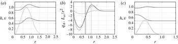
, and the associated infinite gradient would normally be damped by viscosity – if introduced. In practice, it does not affect the results concerning the instability, and numerical simulations of the evolution of such vortices show that they quickly adjust towards a regular shape at the centre without altering the dynamics elsewhere.) Examples of vortex profiles with the parameters to be used below are presented in figure 1.
Vortex profiles (2.5) with
 ${\it\alpha}=3$
,
 ${\it\delta}=1$
,
 $d=0.9$
and
 $\mathit{Ro}=1.4$
for: (a)
 $\mathit{Bu}=2$
,
 ${\it\kappa}=1$
; (b)
 $\mathit{Bu}=2$
,
 ${\it\kappa}=1$
; and (c)
 $\mathit{Bu}=7$
,
 ${\it\kappa}=0.9$
. (a,c) Layer thicknesses (black continuous) with indicated values at rest (black dashed). Absolute value of the velocity is superimposed in grey. (b) PV anomaly in both layers (black) and absolute angular momentum divided by
 $r^{2}$
(grey). Vertical black and grey lines indicate, respectively, the position of maximum velocity and the zone of negative Rayleigh discriminant. Upper layer, continuous; lower layer, dashed (except for the thicknesses).

The non-dimensional linearized equations for the perturbation
 $(u_{i},v_{i},{\it\eta}_{i})$
read:
 $$\begin{eqnarray}\displaystyle & \displaystyle \left(\partial _{t}+\frac{\overline{V_{i}}}{r}\partial _{{\it\theta}}\right)u_{i}-\left(1+2\frac{\overline{V_{i}}}{r}\right)v_{i}+\partial _{r}(d^{i-1}{\it\eta}_{1}+{\it\eta}_{2})=0, & \displaystyle\end{eqnarray}$$
 $$\begin{eqnarray}\displaystyle & \displaystyle \left(\partial _{t}+\frac{\overline{V_{i}}}{r}\partial _{{\it\theta}}\right)v_{i}+\left(1+\frac{\overline{V_{i}}}{r}+\partial _{r}\overline{V_{i}}\right)u_{i}+\frac{1}{r}\partial _{{\it\theta}}(d^{i-1}{\it\eta}_{1}+{\it\eta}_{2})=0, & \displaystyle\end{eqnarray}$$
 $$\begin{eqnarray}\displaystyle & \displaystyle \left(\partial _{t}+\frac{\overline{V_{i}}}{r}\partial _{{\it\theta}}\right){\it\eta}_{i}+\left[\overline{H}_{i}\partial _{r}+\frac{\partial _{r}(r\overline{H}_{i})}{r}\right]u_{i}+\frac{\overline{H}_{i}}{r}\partial _{{\it\theta}}v_{i}=0,\quad i=1,2. & \displaystyle\end{eqnarray}$$
 $(u_{i},v_{i},{\it\eta}_{i})(r,{\it\theta},t)=(\text{i}\tilde{u_{i}},\tilde{v_{i}},\tilde{{\it\eta}_{i}})(r)\,\text{e}^{\text{i}(l{\it\theta}-{\it\omega}t)}$
, where
 $l$
is the discrete azimuthal wavenumber and
 ${\it\omega}$
is the frequency. The system (2.6)–(2.8) can be written, omitting the tildes, in the form
 $$\begin{eqnarray}{\it\omega}\!\left(\begin{array}{@{}c@{}}u_{1}\\ v_{1}\\ {\it\eta}_{1}\\ u_{2}\\ v_{2}\\ {\it\eta}_{2}\end{array}\right)\!=\!\left(\begin{array}{@{}cccccc@{}}l\displaystyle \frac{\overline{V_{1}}}{r}\; & 1+2\displaystyle \frac{\overline{V_{1}}}{r}\; & -\mathscr{D}_{N}\; & 0\; & 0\; & -\mathscr{D}_{N}\\ 1+\displaystyle \frac{\overline{V_{1}}}{r}+\mathscr{D}_{N}\overline{V_{1}}\; & l\displaystyle \frac{\overline{V_{1}}}{r}\; & \displaystyle \frac{l}{r}\; & 0\; & 0\; & \displaystyle \frac{l}{r}\\ \displaystyle \frac{\mathscr{D}_{N}(r\overline{H}_{1})}{r}+\overline{H}_{1}\mathscr{D}_{N}\; & l\displaystyle \frac{\overline{H}_{1}}{r}\; & l\displaystyle \frac{\overline{V_{1}}}{r}\; & 0\; & 0\; & 0\\ 0\; & 0\; & -d\mathscr{D}_{N}\; & l\displaystyle \frac{\overline{V_{2}}}{r}\; & 1+2\displaystyle \frac{\overline{V_{2}}}{r}\; & -\mathscr{D}_{N}\\ 0\; & 0\; & \displaystyle \frac{dl}{r}\; & 1+\displaystyle \frac{\overline{V_{2}}}{r}+\mathscr{D}_{N}\overline{V_{2}}\; & l\displaystyle \frac{\overline{V_{2}}}{r}\; & \displaystyle \frac{l}{r}\\ 0\; & 0\; & 0\; & \displaystyle \frac{\mathscr{D}_{N}(r\overline{H}_{2})}{r}+\overline{H}_{2}\mathscr{D}_{N}\; & l\displaystyle \frac{\overline{H}_{2}}{r}\; & l\displaystyle \frac{\overline{V_{2}}}{r}\end{array}\right)\!\!\left(\begin{array}{@{}c@{}}u_{1}\\ v_{1}\\ {\it\eta}_{1}\\ u_{2}\\ v_{2}\\ {\it\eta}_{2}\end{array}\right)\end{eqnarray}$$
where
 $\mathscr{D}_{N}$
is the operator of differentiation in
 $r$
, which becomes the differentiation matrix when the system is discretized in
 $r$
over an
 $N$
-point grid, which is anticipated in the notation. The details of the discretization procedure and set-up are given in appendix A.
The boundary condition at
 $r\rightarrow 0$
is vanishing of all of the six variables, except for the axisymmetric perturbation with
 $l=0$
for which the condition
 ${\it\eta}_{i}\rightarrow 0$
is replaced by
 $\partial _{r}{\it\eta}_{i}\rightarrow 0$
; and for
 $l=1$
where the proper dynamical condition is
 $u_{i}=-v_{i}$
. There is no specific condition imposed at infinity, but the numerical method we use implies that the solutions are decaying there; see appendix A. We are not introducing dissipation in the linear stability analysis because, as will be shown below, the modes we are mostly interesting in have typical growth rates of the order unity and will be not substantially affected by a weak dissipation. These unstable modes correspond to the gravest modes in continuously stratified fluid, and are usually not significantly affected by viscosity (see e.g. Ribstein et al.
Reference Ribstein, Plougonven and Zeitlin2014). The Ekman damping is not sensitive to the spatial structure of the modes, and thus not selective. It will be not considered, for simplicity.
We will be solving the system (2.9) by the collocation method in order to determine the eigenfrequencies
 ${\it\omega}={\it\omega}_{r}+\text{i}{\it\omega}_{i}$
and corresponding eigenvectors. The imaginary part of the eigenvalue
 ${\it\omega}_{i}\equiv {\it\sigma}$
gives the growth rate of the unstable modes.
In the symmetric case, and for a purely barotropic vortex (
 ${\it\kappa}=1\ \Rightarrow \ \overline{V}_{1}=\overline{V}_{2}=\overline{V}$
), the linear system of equations (2.9) can be reduced, by straightforward elimination of variables, to the following one:
 $$\begin{eqnarray}(-{\it\omega}^{2}+\overline{{\it\Phi}})\left(\begin{array}{@{}c@{}}u_{1}\\ u_{2}\end{array}\right)=\partial _{r}\left(\frac{\partial _{r}}{r}\left(\begin{array}{@{}c@{}}r\overline{H}_{1}u_{1}+r\overline{H}_{2}u_{2}\\ r\,d\overline{H}_{1}u_{1}+r\overline{H}_{2}u_{2}\end{array}\right)\right).\end{eqnarray}$$
Here
 $\overline{{\it\Phi}}=2\overline{L}_{a}\overline{{\it\zeta}}_{a}/r^{2}$
,
 $\overline{L}_{a}=r^{2}/2+r\overline{V}$
is the absolute angular momentum, and
 $\overline{{\it\zeta}}_{a}=1+\partial _{r}(r\overline{V})/r$
is the absolute vorticity of the background vortex. From this system one can deduce, following the similar analysis in the case of inertial instability in Bouchut et al. (Reference Bouchut, Ribstein and Zeitlin2011), a relation between the frequency
 ${\it\omega}$
and the baroclinic and barotropic components of the normal modes, defined as
 $u_{b}=u_{1}-u_{2}$
and
 $u_{B}=(\overline{H}_{1}u_{1}+\overline{H}_{2}u_{2})/\overline{H}_{0}$
, respectively. By multiplying (2.10) by
 $\overline{H}_{eq}u_{b}^{\ast }$
(with
 $\overline{H}_{eq}=\overline{H}_{1}\overline{H}_{2}/(\overline{H}_{1}+\overline{H}_{2})$
) and integrating over the whole domain, supposing that the velocity field vanishes at infinity, i.e. that we are looking for trapped modes, we get
 $$\begin{eqnarray}\displaystyle {\it\omega}^{2} & = & \displaystyle \frac{\displaystyle \int \overline{{\it\Phi}}\cdot \overline{H}_{eq}|u_{b}|^{2}\,\text{d}r}{\displaystyle \int \overline{H}_{eq}|u_{b}|^{2}\,\text{d}r}+(1-d)\frac{\displaystyle \int \left[|\partial _{r}(\overline{H}_{eq}u_{b})|^{2}+\frac{|\overline{H}_{eq}u_{b}|^{2}}{4r^{2}}\right]\text{d}r}{\displaystyle \int \overline{H}_{eq}|u_{b}|^{2}\,\text{d}r}\nonumber\\ \displaystyle & & \displaystyle -\,(1-d)\frac{\displaystyle \int \overline{H}_{eq}u_{b}^{\ast }\partial _{r}\left(\frac{\partial _{r}(r\overline{H}_{1}u_{B})}{r}\right)\text{d}r}{\displaystyle \int \overline{H}_{eq}|u_{b}|^{2}\,\text{d}r}.\end{eqnarray}$$
 $\overline{{\it\Phi}}$
, and the second term is positive-definite. The third term is not sign-definite, but it is the only one containing the barotropic velocity
 $u_{B}$
, and thus vanishes for purely baroclinic modes. Hence we infer, like in the case of inertial instability (Plougonven & Zeitlin Reference Plougonven and Zeitlin2005), that there exist trapped baroclinic modes, such that their frequencies may become imaginary, for sufficiently large negative values of
 $\overline{{\it\Phi}}$
. We thus recover the classical Rayleigh condition for the centrifugal instability,
 $\overline{{\it\Phi}}\propto \overline{L}_{a}\overline{{\it\zeta}}_{a}<0$
, where the last product is the Rayleigh discriminant in our model (cf. Kloosterziel & van Heijst (Reference Kloosterziel and van Heijst1991) for the continuously stratified rotating fluid). The estimate (2.11) for the eigenfrequencies will be used below to control the numerical results for the eigenproblem (2.9) at
 $l=0$
.
3. Results of the linear stability analysis
We start with a detailed stability analysis of the linearized problem in the long-wave sector, i.e. for perturbations with low
 $l$
. The main motivation for this analysis is to find out which instability is dominant as a function of the vortex parameters. Of particular interest is eventual competition between the barotropic and the centrifugal instability, and the existence of non-axisymmetric unstable modes with similar properties as the centrifugal one, as suggested by previous studies (Smyth & McWilliams Reference Smyth and McWilliams1998; Billant & Gallaire Reference Billant and Gallaire2005; Bouchut et al.
Reference Bouchut, Ribstein and Zeitlin2011). We pay particular attention to the impact of the vertical structure (stratification and vertical shear) on the results. As follows from (2.11), these are the anticyclonic vortices, which are prone to centrifugal instability, so we will work with anticyclonic background profiles.
The algebraic system (2.9) is solved with the help of the collocation method, specially adapted for cylindrical geometry and described in appendix A. A similar technique was used previously in Katsman et al. (Reference Katsman, Van Der Vaart, Dijkstra and De Ruijet2003) in a study of the linear stability of large-scale ocean vortices. Most of the results of the linear stability analysis below were obtained with
 $N=160$
collocation points. Numerical convergence has been checked for selected modes by doubling this resolution. Before giving the details in the subsequent subsections we summarize the main results of the linear stability analysis.
For barotropic vortices we have the following:
-
(i) The standard centrifugal instability is dominant at high Rossby (
 ${\gtrsim}0.8$
) and low Burger (
${\lesssim}10$
) numbers and for sufficiently weak stratification and/or depth ratio.
-
(ii) For stronger stratification, the centrifugal mode is no longer the most unstable, irrespective of the values of the Rossby and Burger numbers. The non-axisymmetric mode with the azimuthal wavenumber
$l=1$
is the most unstable at high Rossby and low Burger numbers. It has a structure very close to the symmetric centrifugal instability mode. -
(iii) Regardless of the stratification strength, at least in the range we investigated, the dominant instability mode at high Burger (
${\gtrsim}10$
) and/or low Rossby (
${\lesssim}0.7$
) numbers is barotropic, with azimuthal wavenumber
$l=2$
. -
(iv) In between these two domains (high
$\mathit{Ro}$
–low
$\mathit{Bu}$
and low
$\mathit{Ro}$
–large
$\mathit{Bu}$
) the non-axisymmetric
$l=1$
or
$l=2$
unstable modes have the highest growth rates.


For baroclinic vortices the vertical shear tends to inhibit both axisymmetric and non-axisymmetric centrifugal instabilities and render the barotropic one dominant.
3.1. Barotropic vortices: weakly stratified case,
$d=0.99$

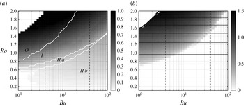
We show in figure 2 the growth rate of the dominant instabilities in the
 $(\mathit{Ro},\mathit{Bu})$
plane for a barotropic vortex (
 ${\it\kappa}=1$
) with moderate horizontal shear:
 ${\it\alpha}=3$
. The anticyclonic vortex is found to be unstable almost everywhere in the plane. The calculations were performed at
 $d=0.99$
,
 ${\it\delta}=1$
and the azimuthal wavenumber
 $l$
in the range
 $[0,4]$
.
Growth rate
 ${\it\sigma}$
of the most unstable modes of the barotropic vortex with
 ${\it\alpha}=3$
,
 $d=0.99$
and
 ${\it\delta}=1$
as a function of Rossby and barotropic Burger numbers. The baroclinic Burger number is
 $\mathit{Bu}^{\prime }\approx \mathit{Bu}/400$
. Values of
 $\mathit{Bu}^{\prime }=0.01$
and 0.1 are marked by black dashed vertical lines. (a) Most unstable modes in the interval
 $l\in [0,4]$
(grey scale is saturated at one), with separation lines in white between the regimes with different most unstable mode:
 $O$
, symmetric centrifugal,
 $l=0$
;
 $I$
, first asymmetric centrifugal,
 $l=1$
;
 $II.a$
, second asymmetric centrifugal,
 $l=2$
; and
 $II.b$
, barotropic,
 $l=2$
. (b) Maximum value of
 ${\it\sigma}$
for the unstable modes with
 $l=0$
(grey) and isopleths (black continuous) of
 $-\overline{{\it\Phi}}$
for the background vortex at 0.1 (lowermost curve) and from 0.25 to 2 (uppermost curve) at the interval 0.25.

Qualitative agreement is found with the value given by the Rayleigh criterion. The zone of dominant symmetric centrifugal instability on figure 2(b) coincides with the zone of strongest negative
 $\overline{{\it\Phi}}$
, except for the dependence on the Burger number, which is not taken into account by the Rayleigh discriminant (but can be understood considering the integral estimate given by (2.11), where the second term on the right-hand side is positive-definite and scales as the Burger number).
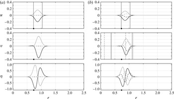
As follows from figure 2(a), the overall highest growth rates correspond to the axisymmetric centrifugal instability. The structure of the corresponding most unstable mode at given values of the vortex parameters is presented in figure 3(a). As expected, its amplitude is radially confined in the zone where the Rayleigh discriminant is negative (Kloosterziel et al.
Reference Kloosterziel, Carnevale and Orlandi2007). The mode is trapped, and it is essentially baroclinic (i.e. with opposite velocities layerwise and strong deviation of the interface) and ageostrophic. This structure is in perfect agreement with what follows from the analysis of the general expression (2.11). We also show in figure 3 the structure of the second most unstable mode, which has an azimuthal wavenumber
 $l=1$
for the same vortex parameters. Strong similarities between the two modes appear: the asymmetric
 $l=1$
mode is clearly trapped in the same zone given by the Rayleigh criterion, and is baroclinic and ageostrophic. We may, thus, infer that the two modes correspond to symmetric and asymmetric versions of the same centrifugal instability. For this reason and by further arguments to come up below, this mode will be referred to as an asymmetric centrifugal instability from now on. We should emphasize that, unlike its symmetric counterpart, the
 $l=1$
centrifugal mode is propagating in the azimuthal direction. It has a critical radius (the radius
 $r_{c}$
at which the phase speed is equal to the background flow velocity), which does not coincide with the location where the PV gradient of the vortex vanishes (even when the growth rate goes to zero); see figure 3. The standard mechanism of the classical baroclinic instability is the resonance between Rossby waves, which implies that the PV gradient must vanish at the critical radius in the limit of vanishing growth rate (i.e. for the neutral waves undergoing phase locking, see Lin (Reference Lin1945) and Iga (Reference Iga1999)). Thus, the asymmetric centrifugal mode cannot be directly related to the classical baroclinic instability, being apparently its ageostrophic generalization.
Structure (amplitude as a function of the radius) of the (a)
 $l=0$
and (b)
 $l=1$
modes of the centrifugal instability at
 $\mathit{Ro}=1.2$
,
 $\mathit{Bu}=2$
,
 ${\it\delta}=1$
,
 ${\it\kappa}=1$
and
 $d=0.99$
. The growth rates of the modes are 0.76 and 0.73, respectively. First row: radial velocity
 $u$
, with two vertical lines indicating the boundaries of the area where the Rayleigh discriminant is negative. Second row: azimuthal velocity
 $v$
, with vertical lines indicating the radius where PV gradient vanishes (black/grey continuous in the upper/lower layer) and the location of the critical radius
 $r_{c}$
(black dashed, if appropriate). Third row: thickness deviation
 ${\it\eta}$
. Continuous, real part; dashed, imaginary part; black, upper layer; grey, lower layer. Bullets on the
 $x$
-axes indicate the location of the velocity maximum in the background flow:
 $r_{max}=\mathit{Bu}^{-1/2}$
.

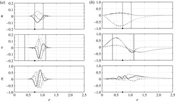
For larger Burger and/or lower Rossby numbers, the second azimuthal mode corresponding to another instability becomes dominant; cf. figure 2. Its structure is presented on figure 4(b). Note that the velocity field of this mode is quasi-barotropic (i.e. the velocities in the upper and the lower layer are very close). The growth rates associated with this instability are weaker and increase with the Burger number, opposite to the centrifugal modes. This mode is almost geostrophically balanced beyond the radius corresponding to the maximum velocity of the background vortex, and has a critical level located at a radius where the PV gradient vanishes; see figure 4. This allows us to interpret this unstable mode as a resonance between two non-singular Rossby waves, the condition of existence of a neutral wave
 $Q^{\prime }(r_{c})=0$
(Lin Reference Lin1945) being fulfilled, and hence we identify this mode as an ageostrophic version of the classical barotropic instability. Furthermore, when the Rossby number decreases, this mode clearly evolves towards the well-known pattern of the quasi-geostrophic barotropic instability (the velocity field verifies the geostrophic balance almost everywhere; not shown). For baroclinic Burger numbers greater than unity (and thus out of the range covered here), the standard baroclinic instability arises.
Structure of (a) the most unstable centrifugal mode and (b) the most unstable barotropic mode with azimuthal wavenumber
 $l=2$
of a vortex with
 $\mathit{Ro}=1.2$
,
 $\mathit{Bu}=2$
,
 ${\it\delta}={\it\kappa}=1$
,
 ${\it\alpha}=3$
and
 $d=0.99$
. The growth rates are 0.6 and 0.1, respectively. Same legend as in figure 3.

On the lower Burger–higher Rossby side of the zone of the dominant barotropic instability we find a strip where the most unstable mode has also the azimuthal wavenumber
 $l=2$
(cf. figure 2
a), but a different structure. As visible in figure 4(a) where this mode is displayed, its radial and vertical structure (trapped in the same zone, baroclinic) is similar to that of the centrifugal instability modes with
 $l=0$
and
 $l=1$
. We thus identify this unstable mode as a second asymmetric centrifugal one with azimuthal wavenumber
 $l=2$
. The phase speeds of all these modes are roughly equal and lie in the range
 $-1.2<{\it\omega}/l<-0.6$
for the parameters of figure 2(a), while the phase speed of the barotropic instability mode is roughly proportional to the (negative) Rossby number and ranges between
 $-1$
and 0.
3.2. Barotropic vortices: increasing stratification
In order to study the impact of stratification on the results obtained in the previous subsection, we repeat the analysis with decreasing
 $d$
. We show in figure 5(a) the growth rates of the dominant instabilities in the
 $(\mathit{Ro},\mathit{Bu})$
plane for a barotropic vortex with
 ${\it\alpha}=3$
,
 ${\it\delta}=1$
and
 $d=0.9$
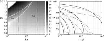
. In sharp contrast with the weakly stratified case, the symmetric centrifugal mode is never the most unstable, albeit its growth rate is close to the one of the leading first azimuthal mode (not shown). This result parallels the recent findings on inertial instability of a Bickley jet in the two-layer shallow water model (Bouchut et al.
Reference Bouchut, Ribstein and Zeitlin2011), where it was shown that asymmetric inertial instability dominates the symmetric one. Similar results hold in a large range of vertical wavenumbers in the full three-dimensional primitive equations (Stevens & Ciesielski Reference Stevens and Ciesielski1986; Arobone & Sarkar Reference Arobone and Sarkar2012; Ribstein et al.
Reference Ribstein, Plougonven and Zeitlin2014). For strongly stratified vortices, an analogous result was found in Smyth & McWilliams (Reference Smyth and McWilliams1998).
(a) Same as in figure 2,
 ${\it\sigma}$
versus
 $\mathit{Bu}$
,
 $\mathit{Ro}$
, but for
 $d=0.9$
. Vertical black dashed lines stand for
 $\mathit{Bu}^{\prime }=0.1$
and 1, from left to right. (b) Evolution of the growth rate of the most unstable modes
 ${\it\sigma}$
as a function of
 $1-d$
, for
 $\mathit{Bu}=2$
,
 $\mathit{Ro}=1.4$
. Black continuous,
 $l=0$
; grey,
 $l=1$
; black dashed,
 $l=2$
. Here
 $l=3$
and weakly unstable
 $l=2$
modes are not shown. The number of nodes in the radial profile of the eigenvector decreases as the growth rate increases at fixed value of
 $d$
.

As follows from figure 5(b), the growth rates of the centrifugal instability modes decrease as the stratification increases. The symmetric mode is more strongly affected by the density ratio, with its growth rate decreasing faster, hence there is a specific value of the density ratio for which the asymmetric centrifugal mode with
 $l=1$
becomes dominant. The above-mentioned dependence is consistent with previous results obtained in the framework of continuously stratified fluid (Smyth & McWilliams Reference Smyth and McWilliams1998; Billant & Gallaire Reference Billant and Gallaire2005; Kloosterziel et al.
Reference Kloosterziel, Carnevale and Orlandi2007), where it was found that the classical centrifugal instability is more active at weak stratifications. This can be explained by the fact that the centrifugal instability generates overturning motions in the vertical
 $(r,z)$
plane, which are inhibited by stratification. The barotropic instability mode is not sensitive to stratification, which implies that the area in the
 $(\mathit{Ro},\mathit{Bu})$
plane where centrifugal modes are dominant is reduced. This is confirmed by comparison of figures 2(a) and 5(a).
As follows from figure 5(b), the number of unstable modes increases with decreasing stratification. The extra axisymmetric modes with
 $l=0$
are higher radial modes of the centrifugal instability with an increasing number of nodes, as expected from the analytic treatment of the symmetric centrifugal instability. (This may be done, following Le Sommer et al. (Reference Le Sommer, Medvedev, Plougonven and Zeitlin2003), by imposing, for simplicity, a rigid lid in the two-layer model and reducing the system to a Schrödinger equation where the anticyclonic shear plays the role of the potential. It follows that unstable trapped modes with more nodes and lower growth rates emerge as the potential well deepens.) We checked that these modes satisfy the integral relation for the growth rate (2.11). The interesting fact is that asymmetric modes of centrifugal instability with more nodes also arise.
It is worth mentioning that the radial extent of the centrifugal modes extends as the stratification strengthens, especially for the larger azimuthal wavenumbers (not shown).
3.3. Barotropic vortices: the impact of the thickness ratio
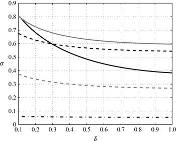
In this subsection we investigate the impact of the ratio of the layer thicknesses. We show in figure 6 the variation of the growth rates of different azimuthal modes with
 ${\it\delta}=H_{1}/H_{2}$
for fixed values of Rossby and Burger numbers, at
 $d=0.9$
and
 ${\it\alpha}=3$
.
Evolution of the growth rate of the unstable modes of a barotropic vortex with
 $\mathit{Ro}=1.4$
and
 $\mathit{Bu}=2$
as a function of
 ${\it\delta}$
. Black continuous,
 $l=0$
centrifugal mode; grey continuous,
 $l=1$
centrifugal mode; black dashed,
 $l=2$
centrifugal mode; black dash-dotted,
 $l=2$
barotropic mode; grey dashed,
 $l=3$
centrifugal mode.

One sees in the figure that the growth rate of the centrifugal modes increases as
 ${\it\delta}$
decreases: the lower the azimuthal wavenumber, the stronger the increase. Thus, for very low values of the thickness ratio the symmetric mode becomes dominant. In the two-layer model, the fact that symmetric modes are more unstable for lower
 ${\it\delta}$
may be considered as selection of higher vertical wavenumber by the instability, well known for centrifugal and inertial instabilities. The vertical structure of the centrifugal modes is clearly surface-intensified as the surface layer thins down, which supports this hypothesis. We observe that the barotropic component of such modes remains very weak, with
 $\overline{H}_{1}u_{1}\approx -\overline{H}_{2}u_{2}$
. Contrary to the centrifugally unstable modes, the growth rate of the unstable mode of the barotropic instability is not very sensitive to the thickness ratio.
3.4. Impact of the vertical shear: baroclinic vortices
Although the barotropic background vortex flows of the previous subsections are most natural for studying the centrifugal instability, which is our primary goal, the model allows for easy incorporation of the baroclinicity of the background flow. We sketch in this subsection the dependence of the stability results on the vertical shear of the background vortex (2.5), which is controlled by the ratio of the maximal velocities in the layers
 ${\it\kappa}=V_{2}/V_{1}$
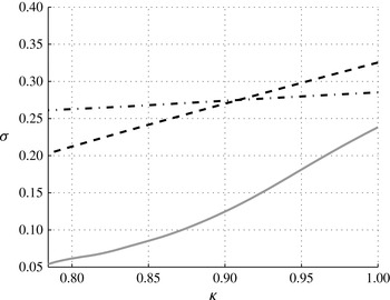
. The evolution of the growth rates of different unstable modes with
 ${\it\kappa}$
is shown in figure 7. Note that
 ${\it\kappa}=1$
corresponds to the barotropic vortex studied in the previous subsections. The results are presented for a larger value of the Burger number
 $\mathit{Bu}=7$
, because of drying of the upper layer at low Burger numbers.
Evolution of the growth rate of the unstable modes of a vortex with
 $\mathit{Ro}=1.4$
,
 $\mathit{Bu}=7$
,
 ${\it\delta}=1$
and
 $d=0.9$
as a function of
 ${\it\kappa}$
. Same legend as in figure 6.

For the parameters of the figure, the vortex is stable with respect to symmetric centrifugal instability. We see that the growth rates of all unstable modes decrease with the vertical shear, and that both centrifugal ones with
 $l=1$
and
 $l=2$
are more sensitive to the vertical shear than the barotropic mode with
 $l=2$
. A swap between dominant instabilities takes place around
 ${\it\kappa}=0.91$
, with barotropic instability becoming the leading one. This fact confirms that the centrifugal instability is most relevant for the barotropic vortices. We should emphasize that the barotropic mode develops a weak vertical shear for
 ${\it\kappa}<1$
(not shown); thus it would be more appropriate to call it mixed (barotropic–baroclinic). However, the velocities remain mainly collinear layerwise and the background vortex is far from the standard baroclinic configuration – generally, confined in one layer – in which the baroclinic instability is usually studied, hence we keep the name ‘barotropic’.
These results show the sensitivity of the stability properties to the vertical structure of the background vortex, and give a rather complicated picture of interchanges between different instabilities, already in the simplest two-layer configuration. Although the growth rates of the centrifugal instability are the highest among all those we observed, we found that, depending on the vertical structure, they may correspond to symmetric or to asymmetric variants of the instability. Moreover, for vortices with sufficient vertical shear, the centrifugal instability may be overcome by the ageostrophic barotropic instability. In practice, this means that a good knowledge of the vertical structure of the flow, besides its Rossby and Burger numbers, is needed in order to understand what processes account for its instability.
4. Nonlinear saturation of the instabilities of anticyclonic vortices
In this section we describe the nonlinear development of the above-identified linearly unstable modes. We have established in the previous section that, in the long-wave sector, the ageostrophic
 ${\it\alpha}$
-Gaussian vortices are unstable with respect to symmetric and asymmetric centrifugal and barotropic instabilities. Each of them can be dominant, depending on the vertical structure of the vortex. Because of differences in the structure of the unstable modes, one can expect different patterns of nonlinear development of these instabilities. Moreover, even if it is the standard symmetric centrifugal instability that is dominant, the vortex can remain unstable with respect to the barotropic instability after the saturation of this latter, and thus undergo a secondary saturation stage, like that observed for inertially unstable jets (Ribstein et al.
Reference Ribstein, Plougonven and Zeitlin2014). We check these expectations in the numerical experiments presented below. We use a high-resolution well-balanced finite-volume scheme (Bouchut & Zeitlin Reference Bouchut and Zeitlin2010) initialized with an
 ${\it\alpha}$
-Gaussian vortex with superimposed unstable mode found from the linear stability analysis with a rather weak amplitude: the maximum of thickness perturbation is about 10 % of the deviation of layer thicknesses in the vortex with respect to the state of rest. In this way, the vortex is forced to destabilize through the chosen mode, even if it is more unstable with respect to other ones. We introduce sponges, which are represented by Neumann boundary conditions, at the boundaries of the computational domain, in order to prevent the inertia–gravity waves emitted in the course of evolution from coming back. The correspondence of the linear stability and numerical simulations results serves to benchmark the numerical scheme. It is checked by comparing the growth rate of the perturbation in the initial stages of simulations, measured by the mean absolute value of the upper-layer pressure anomaly (or by the energy of the perturbation), with the growth rate obtained from the linear stability analysis. We always find good agreement between the two, for all of the instabilities in question, which means that the differences in boundary conditions between linear stability analysis and direct numerical simulation are inessential for the strongly localized unstable modes in which we are interested.
4.1. Saturation of symmetric and asymmetric centrifugal instabilities
We first present the results of the nonlinear development of the centrifugal instability for the two values of the azimuthal wavenumber corresponding to the highest growth rates,
 $l=0$
and
 $l=1$
. As is known, in a three-dimensional continuously stratified fluid, the evolving centrifugal instability gives rise to overturning motions in the vertical plane, redistributing the angular momentum, enhancing dissipation and leading to the emission of inertia–gravity waves. These processes lead to homogenization of the flow in the zone of initial instability (i.e. where the Rayleigh discriminant is negative) and to a marginally stable vortex profile, as shown in Kloosterziel et al. (Reference Kloosterziel, Carnevale and Orlandi2007) for strictly axisymmetric configurations. The mean flow stayed a fortiori monopolar in the course of its destabilization in this study. It remains unknown how this behaviour changes if the strict axisymmetry constraint is relaxed.
Although, by construction of the two-layer model by vertical averaging, the overturning motions are not accessible, the intense vertical shears and related strong baroclinic divergence are well detectable. As was checked on multiple examples with our numerical code (e.g. Bouchut et al. Reference Bouchut, Ribstein and Zeitlin2011), the Kelvin–Helmholtz-like instabilities associated with strong vertical shear, and eventually with overturning, are accounted for by the hyperbolicity loss of the flow in the corresponding locations. One should, however, keep in mind that this mechanism does not lead to inter-layer mixing. The numerical scheme has a very satisfactory behaviour under such conditions (Bouchut & Zeitlin Reference Bouchut and Zeitlin2010): non-hyperbolic regions, once they have appeared, remain spatially confined and eventually vanish, and the related strong gradients are wiped out by enhanced numerical dissipation in these locations, as should be the case for an authentic Kelvin–Helmholtz instability.
The hyperbolicity loss thus can be regarded as a proxy for overturning motions and vertical mixing. The corresponding regions of the flow are the main zones of energy dissipation (see below). Furthermore, the numerical scheme is based on the conservative form of (2.1) and (2.2) and conserves exactly the mass layerwise, together with the total momentum. Good conservation of the PV is always observed, albeit it is not explicitly built in to the code. The total mass conservation has been checked in all the numerical simulations we present. The relative departure of the mass averaged over all numerical cells is approximately
 $10^{-4}$
at
 $t=100\,f^{-1}$
and is mainly due to the imperfect sponges when high-amplitude waves reach the boundaries. If periodic boundary conditions are used, this value falls to
 $10^{-14}$
. We should also emphasize that, in spite of its two-dimensional character, the model does give access to vertical velocity, which is proportional to the horizontal convergence, by construction.
The simulations described below have been performed with the following vortex parameters:
 ${\it\delta}=1$
,
 ${\it\kappa}=1$
,
 $d=0.9$
and
 ${\it\alpha}=3$
. The Rossby and Burger numbers are respectively 1.5 and 2, and the growth rates of the unstable modes used for initializations are 0.55 for the
 $l=0$
and 0.7 for the
 $l=1$
mode, for this choice of parameters. In all simulations, we did not observe the formation of a new stable vortex, as a result of the nonlinear saturation. For initializations with both
 $l=0$
and
 $l=1$
modes of the centrifugal instability, the initial vortex totally breaks down. It rapidly develops strong vertical shears (the baroclinic component of velocity grows and rapidly exceeds the phase velocity of the baroclinic waves), while the barotropic velocity weakens.
4.1.1. Nonlinear saturation of the symmetric centrifugal instability
The classical symmetric centrifugal instability is the one for which high-resolution numerical simulations of the saturation exist in the full three-dimensional configuration, yet under the constraint of strict axisymmetry (Kloosterziel et al.
Reference Kloosterziel, Carnevale and Orlandi2007) or neutral stratification (Orlandi & Carnevale Reference Orlandi and Carnevale1999). They predict the flow to become marginally stable with
 $L_{a}{\it\zeta}_{a}\geqslant 0$
everywhere. The evolution of an initially symmetric perturbation with
 $l=0$
that we observe in the two-layer model confirms this scenario at initial stages. The flow remains globally axisymmetric until
 $t\approx 5$
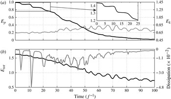
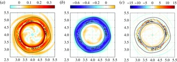
. As follows from figure 8, where we present the evolution of the energy, the dissipation is already active at this stage of the saturation. Figure 9, where we present the distributions of the divergence and of both components of the baroclinic velocity, shows that the zone of hyperbolicity loss is axisymmetric. Typical small-scale structures, characteristic of the saturation of the centrifugal and inertial instabilities, are visible in the figure and are associated with the major part of the energy dissipation. One can nevertheless infer a weak
 $l=4$
modulation (e.g. in the magnitude of the ripples visible in the baroclinic divergence field), which can be traced back to the very beginning of the simulation and is, most probably, due to discretization errors. (We should emphasize that discretization errors in representing a circle with a Cartesian grid are universal, unless polar coordinates are used, which would add substantially complexity to the numerical scheme.)
Saturation of the axisymmetric centrifugal instability. (a) The kinetic energy (black, right axis) and the anomaly of potential energy (grey, left axis). (b) Total energy anomaly (black, left axis) and dissipation calculated cellwise and summed over all cells (grey, right axis).

Snapshots of the (a) radial and (b) azimuthal baroclinic velocities, and of the (c) baroclinic divergence during the nonlinear saturation of the axisymmetric instability at
 $t=3.5\,f^{-1}$
. Non-hyperbolic zones are confined in the annulus between thin contours.

It is to be emphasized that the evolution of the flow at this stage, which corresponds to the first significant drop of energy at
 $t\approx 5$
(cf. figure 8
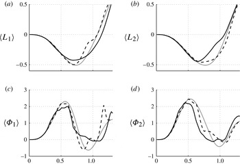
a), follows the scenario of Kloosterziel et al. (Reference Kloosterziel, Carnevale and Orlandi2007), as the flow restabilizes with respect to the Rayleigh criterion, as follows from figure 10. This can be considered as a benchmark of our numerical code.
Evolution of the azimuthal averages of the (a,b) angular momentum and (c,d) Rayleigh discriminant in the (a,c) upper and (b,d) lower layers, during the nonlinear saturation of the axisymmetric centrifugal instability. The various curves correspond to
 $t=0\,f^{-1}$
(grey),
 $t=8\,f^{-1}$
after the first hyperbolicity loss episode (black dashed), and
 $t=18\,f^{-1}$
after the second one (black continuous).

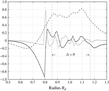
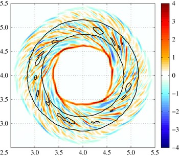
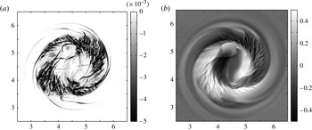
However, the quasi-axisymmetric evolution does not last. A sharp front (shock) with a corresponding jump of radial velocity is formed close to the inner boundary of the non-hyperbolic zone, as shown in figure 11. This front propagates inwards while losing its axial symmetry, as can be seen from figure 12.
Saturation of the axisymmetric centrifugal instability: radial distribution of the radial and azimuthal components of the baroclinic velocity, and of its divergence, at a given polar angle at
 $t=4.5\,f^{-1}$
.

Saturation of the axisymmetric centrifugal instability: divergence of the baroclinic velocity at
 $t=6\,f^{-1}$
. The contour of high divergence corresponds to the inward-propagating front. Thin black lines delimit the zone of hyperbolicity loss.

Although the quadrupolar perturbation with
 $l=4$
of this inner front in the present simulation is probably triggered by the above-mentioned discretization errors, the instability of axisymmetric concentric shocks propagating towards the centre with respect to non-axisymmetric perturbation is universal (cf. Whitham Reference Whitham1974). So, subject to any non-axisymmetric noise, the front will lose its axial symmetry, and hence the phenomenon we observe is generic.
The second significant drop of energy at
 $t\approx 11$
is related to the reappearance of a non-hyperbolic zone and generation of a new sharp front close to its inner boundary, as shown in figure 13.
Same as in figure 9 but at the beginning of the second hyperbolicity loss episode, at
 $t=11.5\,f^{-1}$
.

As follows from the figure, the flow evolves on the background of the
 $l=4$
structure in the inner core inherited from the preceding stage. It is worth mentioning that non-stationary perturbation due to this inner quadrupolar structure is instantaneously transmitted to the outer boundary of the non-hyperbolic zone, where it leads to the emission of inertia–gravity waves with the same azimuthal structure. Such behaviour is fully consistent with the elliptic nature of the non-hyperbolic zone, where the speed of a signal is infinite, and thus confirms that the numerical scheme is consistent with the underlying physics. The origin of the second dissipation burst is due to the fact that the structure of the centrifugally unstable mode (cf. figure 3), with its strong shear in radial velocity, is not wiped out during the first dissipation burst, and re-creates the conditions of the hyperbolicity loss.
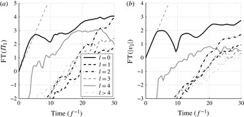
The loss of axisymmetry of the vortex in the course of the evolution of the axisymmetric centrifugal instability is clearly seen in figure 14, where we present the results of the Fourier analysis of pressure and velocity perturbation in the upper layer. The growth of the
 $l=4$
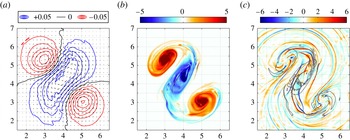
mode eventually leads to the formation of four cyclonic satellites of the main anticyclonic vortex, which subsequently merge pairwise (see the dominance of the
 $l=2$
mode in the Fourier analysis in figure 14, starting at
 $t\approx 25$
). Thus, after the stage of strong local mixing, wave emission and energy dissipation, the flow reorganizes itself, with a weak conversion from kinetic to potential energy (cf. figure 8
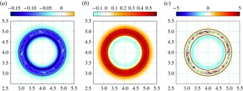
b), into a barotropic tripolar vortex with anticyclonic core, which persists from approximately
 $t=40$
for several tens of inertial periods. This tripole is shown in figure 15. It is not steady: the whole structure rotates rather steadily about the centre, but the distance between the core and the satellites oscillates in time, the core being alternately closer to one or another satellite. It finally splits into a barotropic dipole that slowly goes away from the remaining cyclonic monopole. The flow is still highly energetic, with strong baroclinic shear and associated transient hyperbolicity loss patches. The emission of high-amplitude baroclinic waves continues until the end of the simulation (
 $t=100$
), and kinetic energy is being steadily dissipated (cf. figure 8). The evacuation of the waves from the numerical domain by the Neumann boundary conditions is not perfect and produces spurious oscillations of the potential energy, which are reflected in the total energy evolution. However, the numerical dissipation cellwise summed over all cells inside the numerical domain is negative, as visible in figure 8(b).
Logarithm of the normalized amplitude of the first seven Fourier modes of the upper-layer (a) pressure and (b) velocity perturbations in the course of the evolution of the
 $l=0$
centrifugal instability. The thin black dashed line represents the growth predicted by the linear stability analysis. The burst of
 $l=4$
mode is clearly seen. Its initial amplitude is very small and consistent with the values of discretization errors, and its growth is delayed in time, which confirms its relation to the secondary structures appearing in the course of evolution.

Barotropic tripole formed after nonlinear saturation of the symmetric centrifugal instability at
 $t=60\,f^{-1}$
. (a) Pressure in layer one and superimposed barotropic velocity field. (b) PV anomaly in layer one. Colours are saturated at
 $\pm 5$
(maximum values reach 8). These two fields are similar in the lower layer (not shown). (c) Baroclinic divergence (colours saturated at
 $\pm 6$
) with PV anomaly
 $\pm 1$
isolines in grey superimposed in order to visualize the vortex tripole.

One has to be careful in interpreting these results. Indeed, it is obvious that, because of hyperbolicity loss, the results should be sensitive to the resolution. We checked the numerical convergence by making three different numerical experiments with grid cell sizes varying between
 $0.01R_{d}$
and
 $0.0275R_{d}$
. The saturation process does not change significantly with resolution, only the smallest-scale patterns being modified, as expected. However, the rate of the process changes (the formation of the cyclonic satellites occurs slightly later with the coarser resolution), so we do not achieve numerical convergence, strictly speaking. Nevertheless, the impact of the small-scale processes is sufficiently well resolved to trust the global evolution of the flow that we observe. As we explained above, the mechanism of the observed loss of axial symmetry during the simulation is due to the universal property of destabilization of the concentric inward-propagating front. Although its
 $l=4$
structure is, most probably, due to discretization errors, the mechanism of axial symmetry loss is generic. We should mention that the appearance of
 $l=4$
noise is inherent to the projection of circular structures onto a rectangular grid and thus will appear in any numerical scheme that uses the latter. Finally, let us note that we are not aware of the existence of a three-dimensional analogue of such a phenomenon, which would be interesting to check in high-resolution three-dimensional simulations with step-like stratification and small aspect ratio. Such simulations remain a technical challenge.
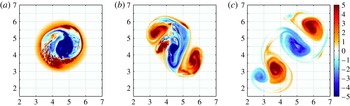
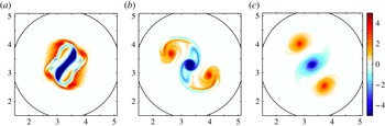
Snapshots of PV anomaly in the upper layer during the nonlinear saturation of the
 $l=1$
centrifugal instability: (a)
 $t=10$
; (b)
 $t=20$
; (c)
 $t=40$
. Colours are saturated at the maximal values indicated on the colour bar for better visibility.

4.1.2. Nonlinear saturation of the asymmetric centrifugal instability
The nonlinear development of the asymmetric
 $l=1$
centrifugal instability exhibits some similarity with the saturation of the symmetric mode, although the end result of the evolution is different. We show snapshots of the evolution of PV in the upper layer (it evolves qualitatively in the same way in the lower layer) in figure 16. The zone of high shear, associated hyperbolicity loss and strong mixing and dissipation also forms, but is now clearly non-axisymmetric, enhanced at either side of the vortex and rotating with it, as shown in figure 17. It is reflected by a mixing zone in the PV anomaly pattern, which roughly coincides with a zone of very low value of the thickness of the corresponding layer, close to incropping. This is visible at
 $t=10$
in figure 16, on the lower left side of the anticyclonic core, and in figure 17, where the high values of the thickness of the lower layer (i.e. the deviation of the interface) are associated with very low values of the upper-layer thickness (the deviation of the free surface being weak). Unlike the
 $l=0$
destabilization (see the inset in figure 8), there are no ‘bursts’ of dissipation (not shown). The original vortex deforms more and more, and finally splits into a well-formed barotropic dipole (upper right corner of figure 16
c), plus a cyclone with a weak anticyclonic satellite (lower left corner; the anticyclone is even weaker in the lower layer). This vortex breaking occurs slightly earlier than the satellite formation in the case of saturating symmetric instability. After
 $t=50$
, the cyclone of the asymmetric dipole remains close to the other dipole, and the anticyclonic monopole stays in the vicinity of this tripolar-like structure. The simulation stops before we can say whether such structure is robust or not. For both
 $l=0$
and
 $l=1$
saturations, the energy balance is comparable: the total amount of kinetic energy dissipated at the end of the simulation (
 $t=100\,f^{-1}$
) accounts for approximately 70 % of the initial value, which is obviously considerable. This amount is almost insensitive to the numerical resolution (it varies from 67 to 70 % for the range of cell sizes we used). We note however that the dissipated kinetic energy is larger for the
 $l=1$
destabilization at the intermediate time
 $t=50$
(
 ${\sim}60$
versus
 ${\sim}50\,\%$
), in agreement with the fact that the vortex breaking occurs earlier than in the
 $l=0$
case and that the growth rate of the initial perturbation is larger.
(a) Numerical dissipation and (b) lower-layer thickness anomaly during the nonlinear saturation of the
 $l=1$
centrifugal instability, at
 $t=10$
. Greyscales are saturated at the maximal values indicated on the bars. High values of the lower-layer thickness anomaly are associated with low values of the upper one, and vice versa. The axes are different with respect to figure 16 for better visibility.

In addition, we simulated the nonlinear development of the asymmetric centrifugal instability with the unstable
 $l=1$
mode for a vortex with smoother horizontal profile:
 ${\it\alpha}=2$
. It corresponds to the classical Gaussian vortex profile, which has been extensively used in the literature on oceanic vortex modelling (e.g. Smyth & McWilliams Reference Smyth and McWilliams1998; Baey & Carton Reference Baey and Carton2002; Benilov Reference Benilov2003, Reference Benilov2004). As follows from the linear stability analysis above, the instabilities are weaker when the horizontal shear decreases, and the vortex is no longer unstable with respect to symmetric perturbations at the same values of the parameters
 ${\it\delta},{\it\kappa}$
and
 $d$
, whereas the
 $l=1$
mode is still unstable with the growth rate
 ${\it\sigma}=0.52$
. The nonlinear evolution of such a vortex (not shown) is different with respect to what is observed for the
 ${\it\alpha}=3$
vortex. Instead of rapidly splitting into a dipole and a monopole, the ring of positive vorticity surrounding the anticyclonic core steadily reorganizes into two cyclonic satellites (although hyperbolicity loss, wave emission and local thinning of the layers are still observed), the final state consisting of a barotropic tripole with an anticyclonic core – which is similar to the nonlinear saturation of the
 $l=0$
mode for
 ${\it\alpha}=3$
. However, baroclinic wave emission is weaker in this case, hyperbolicity loss events are rare and less intense, and only 25 % of the kinetic energy is dissipated at
 $t=100$
(20 % at
 $t=50$
), which is less than half of the corresponding amount in the simulations with
 ${\it\alpha}=3$
presented above.
4.2. Comparison of the saturation of centrifugal and barotropic instabilities
As shown by the linear stability analysis, centrifugal instabilities rapidly disappear when the Burger number increases at fixed Rossby numbers
 $\mathit{Ro}\in [0,2]$
, or when the Rossby number decreases. On the other hand, ageostrophic barotropic and baroclinic (which appears for even larger Burger numbers than those presented) instabilities arise. Our linear stability analysis revealed that the
 $l=2$
barotropic instability is dominant in the major part of the explored
 $\mathit{Ro}$
,
 $\mathit{Bu}$
,
 ${\it\delta}$
,
 ${\it\kappa}$
domain in this case. As is known, nonlinear saturation of the barotropic instability, for moderate Rossby numbers, leads to the formation of either a vortex tripole, or a pair of vortex dipoles, without the production of significant vertical shear, and weak emission of inertia–gravity waves (see e.g. Baey & Carton Reference Baey and Carton2002). On the other hand, as we have seen in § 4.1, the centrifugal instability is associated with strong vertical shear and wave emission.
We thus seek to quantify the differences between the nonlinear saturation of the two instabilities. For this purpose, we selected the unstable modes of a vortex with
 $\mathit{Ro}=1.4$
,
 $\mathit{Bu}=7$
,
 ${\it\alpha}=3$
,
 $d=0.9$
and
 ${\it\delta}={\it\kappa}=1$
. For these values of parameters, the most unstable mode is the
 $l=2$
centrifugal (
 ${\it\sigma}=0.33$
), the second one is the
 $l=2$
barotropic (
 ${\it\sigma}=0.29$
) and the less unstable one of the three is the
 $l=1$
centrifugal (
 ${\it\sigma}=0.24$
). So the asymmetric centrifugal and the barotropic unstable modes have the same azimuthal structure and close growth rates, and it is interesting to compare their respective saturations.
Evolution of the PV anomaly in the upper layer during the nonlinear saturation of the
 $l=2$
centrifugal instability with
 $\mathit{Ro}=1.4$
and
 $\mathit{Bu}=7$
, at (a)
 $t=24\,f^{-1}$
, (b)
 $t=48\,f^{-1}$
and (c)
 $t=100\,f^{-1}$
. The lower-layer PV anomaly is qualitatively similar. Black circle with radius
 ${\approx}1.9R_{d}$
indicates the zone of confinement of the PV anomaly and is used for the diagnostic of wave emission – see text.

Normalized integral of the positive (black) and negative (grey) potential vorticity anomalies (summed over the two layers) as a function of time for the (a)
 $l=2$
centrifugal and (b)
 $l=2$
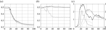
barotropic instabilities. Curves from the simulations of the initial destabilization and the subsequent evolution calculated in a refreshed numerical domain, in order to eliminate spurious reflections of high-amplitude waves by the boundaries, are superimposed for the centrifugal instability. (c) Comparison of the magnitude of the baroclinic divergence inside (black, right axis) and outside (grey, left axis) a circle of radius
 ${\approx}1.9R_{d}$
for the
 $l=2$
centrifugal (continuous) and barotropic (dashed) instabilities.

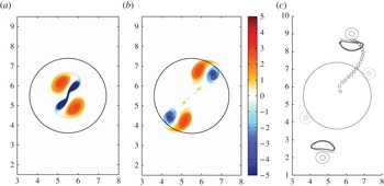
Evolution of the PV anomaly during nonlinear saturation of the barotropic instability for the anticyclone with
 $\mathit{Ro}=1.4$
and
 $\mathit{Bu}=7$
. (a,b) Upper-layer PV anomaly at
 $t=18$
and 30. Up to
 $t\approx 30$
the lower-layer PV anomaly is similar. (c) PV anomaly in the upper (continuous) and lower (dotted) layers at
 $t=70$
, with negative values in grey and positive ones in black, at the interval 1 starting from 0.5 in non-dimensional terms. Previous positions of one of the upper-layer dipoles at time interval 3 are indicated by circles. Black circle indicates the zone of confinement of the PV anomaly in the centrifugal instability case; cf. figure 18.

First of all, we found that the end results of the nonlinear development of the two instabilities are different. The most unstable centrifugal mode evolves into a stable tripole, while the barotropically unstable one gives dipoles (at first barotropic, and then baroclinic ones, see below). However, during the formation of the tripole by the evolving asymmetric centrifugal instability, a saddle point almost forms in the anticyclonic core, which is thus close to splitting (probably into two dipoles – see Arai & Yamagata (Reference Arai and Yamagata1994)), but the vortex finally comes back to a tripolar form, as shown in figure 18. Such an event induces a strong stretching of the anticyclone associated with the vorticity shear, which continues once the tripole has formed. The final structure seems to be stable (the simulation ends at
 $t=140$
) but the magnitude of the vortex, as measured by the integral of the absolute value of the PV anomaly, decreases significantly (see figure 19
a). This contrasts with the case for the development of the barotropic instability, which is shown in figure 20: in this case the splitting of the initial vortex into two barotropic dipoles occurs around
 $t=20$
and we observe a small rise in the integral of the negative PV anomaly (see figure 19
b) while the overall dissipation of the anticyclonic PV anomaly is weaker than in the case of the centrifugal instabilities. The positive (cyclonic) PV anomaly is approximately conserved. The barotropic dipoles are not stable: after ejection of the lower anticyclonic vortex, the dipoles become essentially baroclinic (two-layer cyclone plus upper-layer anticyclone). Such a ‘rider modon’ was reported in the two-layer shallow water model by Lahaye & Zeitlin (Reference Lahaye and Zeitlin2012). The first-stage barotropic and subsequent baroclinic dipoles do not dissipate PV, while the tripole does (through weak but continuous filamentation of the patches). The kinetic energy of the flow exhibits roughly the same behaviour (not shown).
There is, thus, a net difference between the nonlinear development of the
 $l=2$
centrifugal and barotropic instabilities, as regards the redistribution of PV. The latter instability acts to drive away the initial PV anomalies, while the former leads to the formation of a barotropic tripole, which stays at the initial location.
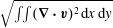
The evolution of the baroclinic divergence field also exhibits striking differences, as shown in figure 19(c), where we compute the square root of the square of divergence integrated over the domain
 $\sqrt{\iint (\boldsymbol{{\rm\nabla}}\boldsymbol{\cdot }\boldsymbol{ v})^{2}\,\text{d}x\,\text{d}y}$
inside and outside a circle delimiting the initial vortex (and the resulting tripole in the centrifugal case; see figure 18). As the initial vortex is essentially ageostrophic, the associated divergence field may correspond to emission of outgoing inertia–gravity waves, or may be proper to the vortex. The two cases may be distinguished by comparing the signals inside and outside the vortex boundary. A persistent emission of large-amplitude inertia–gravity waves is observed during nonlinear saturation of the centrifugal instability, as in the cases with
 $\mathit{Bu}=2$
shown previously. As is clear from figure 19, the waves emitted in the zone of confinement of the PV anomaly propagate outside in this case. With respect to the barotropic instability, the intensity of the divergence is clearly weaker than for the centrifugal instability. The radiation of waves is triggered at
 $t\approx 20$
and lasts up to
 $t\approx 28$
, when the waves go outside of the vortex boundary, which corresponds to the increase (decrease) of the signal in the outer (inner) zone starting at
 $t\approx 24$
. The secondary peak in the signal in the outer zone (
 $t\approx 32$
) is associated with boundary crossing by the secondary dipoles (see figure 20). Once the dipoles have formed, they have an attached divergence field, without wave radiation (not shown). Thus the generation of vertical motions and waves is more important and persistent in the case of the centrifugal instability, whereas it is localized in time for the barotropic one. This is natural, since the former is known to generate overturning motions and waves, whereas the latter is rather two-dimensional (as is clearly visible in the radial structure of the modes; see figure 4). We should stress that the above-established differences in the saturation of the instabilities, which can compete, render predictions of the end states of vortex destabilization highly sensitive to the initial conditions and parameters.
5. Summary and discussion
We have performed a detailed linear stability analysis of essentially ageostrophic anticyclonic two-layer vortices with respect to long-wave azimuthal perturbations, and fully nonlinear numerical simulations of the saturation of the thus identified instabilities.
The linear stability analysis shows that for sufficiently weak stratification the symmetric centrifugal instability is dominant for high Rossby and low Burger numbers. At lower Rossby or larger Burger numbers, the unstable modes with higher wavenumbers (
 $l=1,2$
with our parameters) become dominant. They are non-axisymmetric forms of the classical axisymmetric centrifugal instability. For even higher Burger numbers and/or lower Rossby numbers, there is a swap in the instabilities and the (ageostrophic) barotropic instability with azimuthal wavenumber
 $l=2$
becomes dominant. We found that increasing stratification tends to weaken the centrifugal instabilities, especially the symmetric one, which eventually disappears, while the whole domain of centrifugal instability diminishes in favour of the barotropic one in the
 $\mathit{Ro}{-}\mathit{Bu}$
plane. Vertical shear (
 $=$
baroclinicity) of the vortex has roughly the same effect.
Our main findings, thus, are that in a wide range of parameters the classical symmetric centrifugal instability is dominated by its asymmetric counterpart, that both symmetric and asymmetric instabilities are dominated by the (ageostrophic) barotropic one for sufficiently stratified and/or vertically sheared vortices, and that the details of the vertical structure are crucial to determine which instability is the leading one.
The asymmetric extension of the classical centrifugal instability may seem counter-intuitive: indeed, the initial physical argument invoked to explain the centrifugal instability (conservation of total angular momentum through exchange of rings of fluids (e.g. Rayleigh Reference Rayleigh1917; Drazin & Reid Reference Drazin and Reid1981)) is not directly transposable to asymmetric perturbations. However, we show that the modes that we identified as corresponding to asymmetric centrifugal instability are very close, both in structure and in the scenario of their nonlinear saturation, to the classical modes of centrifugal instability. We should stress that the results obtained by the Wentzel–Kramers–Brillouin–Jeffreys (WKBJ) method for continuously stratified vortices (Billant & Gallaire Reference Billant and Gallaire2005) have already provided a link between asymmetric and symmetric modes, and that similar results (Stevens & Ciesielski Reference Stevens and Ciesielski1986; Bouchut et al. Reference Bouchut, Ribstein and Zeitlin2011) were obtained on inertial instability, which is the counterpart of the centrifugal instability for plane-parallel flows.
An important question, with respect to the linear stability analysis in the two-layer RSW, is how its results are related to those of the full continuously stratified model. We should stress that such results, for vortices with non-trivial stratification and/or vertical shear, are not presently available owing to the technical complexity of the problem, which becomes non-separable in this case.
Our simulations of the nonlinear saturation of centrifugal instability revealed both the expected and new features. Indeed, while the classical picture of kinetic energy dissipation through overturning motions (albeit not explicitly resolved in this model) was reproduced, as well as the recovery of the marginal stability according to the Rayleigh criterion, at some intermediate stage of the evolution, as predicted by Kloosterziel et al. (Reference Kloosterziel, Carnevale and Orlandi2007), the end state was never axisymmetric, unlike in Kloosterziel et al. (Reference Kloosterziel, Carnevale and Orlandi2007) and Lazar et al. (Reference Lazar, Stegner, Caldeira, Dong, Didelle and Viboud2013a ). We observed that, in the course of nonlinear evolution of the symmetric centrifugal instability, the axial symmetry is broken, leading to the formation of either a barotropic tripole or a dipole plus an isolated monopole. We identified an essentially nonlinear mechanism of such symmetry breaking, related to the instability of the front forming at the inner boundary of the mixing zone and propagating inwards.
The asymmetric centrifugal and barotropic instability modes with the same azimuthal wavenumber and vortex parameters evolve differently, the latter leading to the formation of a pair of counter-propagating dipoles while the former gives rise to a quasi-stationary barotropic tripole. Saturation of the barotropic instability leads to weaker energy and potential vorticity dissipation and inertia–gravity wave emission, and smaller amplitudes of the baroclinic divergence field for the resulting structures. We should stress the difference between the two scenarios of saturation, which is important for applications: while in the first one the PV anomalies stay at the same location, they are evacuated by propagating dipoles in the second one. Thus, a small change of the background vortex parameters can produce a switch from one scenario to another, with an obvious impact upon predictability.
Thus, our main conclusion is that two-layer ageostrophic anticyclonic vortices are subject to both barotropic and centrifugal instabilities, the latter not necessarily symmetric. These instabilities may compete, each of them leading to its proper saturation pattern. The symmetric instability generally loses symmetry in the course of nonlinear saturation. Both the character of the dominant instability and the scenario of its nonlinear saturation crucially depend on the vertical structure (shear and stratification) of the flow.
Let us finally comment on the relation of our results to the development of instabilities in a configuration with a stepwise profile of stratification in the fully three-dimensional rotating continuously stratified primitive equations model. As we already mentioned in the Introduction, the problem becomes inseparable, and thus very complex with respect to the linear stability analysis. We are not aware of such results, nor of corresponding high-resolution direct numerical simulations, which are also difficult to realize owing to the coexistence of very different vertical scales in the problem from the very beginning. Laboratory experiments with quasi-two-layer flows at high Rossby numbers (e.g. Flór, Scolan & Gula Reference Flór, Scolan and Gula2011) may provide a key, but the results there are contaminated by ageostrophic instabilities due to the presence of boundaries and related Kelvin waves. However, with respect to the baroclinic ageostrophic Rossby–Kelvin instabilities, the two-layer model gives a reliable description of what is observed in laboratory experiments (Flór et al. Reference Flór, Scolan and Gula2011; Gula & Zeitlin Reference Gula, Zeitlin, von Larcher and Williams2014). We can hypothesize that the results presented above are relevant for the development of the most important modes of the instability, while small-scale modes will be damped by viscosity, as observed for the inertial instability in Ribstein et al. (Reference Ribstein, Plougonven and Zeitlin2014). Of course, only high-resolution numerical simulations of the full continuously stratified equations could validate (or invalidate) this hypothesis. Such simulations, which remain a technical challenge, will have to answer the following questions: (a) how the vertical mode selection operates in the case of the centrifugal instability of vortices with step-like stratification and vertical shear; and (b) under what conditions the vertical mixing introduced by the instability is confined in the zones of sharp density gradient, and dissipation is localized in narrow fronts (shocks), as modelled by the two-layer RSW.
Acknowledgements
This work was supported by the French ANR grant SVEMO. The authors are grateful to F. Bouchut for helpful discussions of the numerical simulations and to the anonymous reviewer who drew their attention to the interpretation of the evolution of the quadrupolar mode. N.L. is grateful to M. Jardak for help with collocation methods.
Appendix A. Collocation method in cylindrical geometry
To solve the linear stability problem, we use the pseudospectral collocation method. Collocation methods rely on interpolation at selected points using an ad hoc orthogonal set of basis functions, with the remainder of the interpolation being strictly zero at the grid points. Chebyshev polynomials are routinely used in order to avoid the Runge phenomenon (spurious oscillations growing in amplitude with the resolution) when interpolating non-periodic functions on a finite non-dimensional interval
 $[-1,1]$
(e.g. Trefethen Reference Trefethen2000; Boyd Reference Boyd2001). However, the cylindrical geometry of the problem treated in the present paper suggests the use of a basis on the interval
 $[0,\infty ]$
. We choose the orthogonal rational functions on a semi-infinite interval
 $TL_{n}$
introduced in Boyd (Reference Boyd1987). They are obtained by applying an algebraic mapping from
 $[-1,1]$
to
 $[0,\infty ]$
to Chebyshev polynomials (we recall that Chebyshev polynomials themselves are the images of the terms of a Fourier cosine series under the mapping
 $x=\cos (t)$
), and are defined by
 $$\begin{eqnarray}TL_{n}(r)=T_{n}(x)=\cos (nt),\end{eqnarray}$$
where
 $t\in [0,{\rm\pi}]$
is the argument of the cosines,
 $x\in [-1,1]$
the argument of the ordinary Chebyshev polynomials
 $T_{n}$
and
 $r\in [0,+\infty ]$
the argument of the new basis functions. The three arguments are related by
 $$\begin{eqnarray}r\equiv L\,\frac{1+x}{1-x}\equiv L\cot ^{2}\left(\frac{t}{2}\right),\end{eqnarray}$$
where
 $L$
is a constant map parameter. In practice, half of the grid points are within the interval
 $[0,L]$
, and the grid is being refined at
 $r\rightarrow 0$
, while the intervals increase for large
 $r$
. This is appropriate, considering that we expect our solutions to decay at infinity. An advantage of this method, as discussed in Boyd (Reference Boyd2001), is that the boundary condition at the upper endpoint of the domain (i.e. infinity) becomes ‘natural’ or ‘behavioural’. This means that the series (the numerical solution) will automatically be bounded at infinity with no need to prescribe any value, following the boundedness of the basis functions there. This is true, in particular, when the differential equation(s) is(are) singular at infinity, although a general theorem is lacking. A drawback of this choice of basis functions is that oscillating functions decaying slowly (not exponentially) at infinity, although not excluded, are poorly resolved: the error becomes large at
 $r\rightarrow \infty$
because the interval between a pair of grid points becomes larger than the wavelength. Solutions to this problem would be either to use the radiation conditions or a modified basis (Boyd Reference Boyd1987, Reference Boyd2001). Taking into account that we are mostly interested in the modes trapped in the vortex, which are responsible for the centrifugal instability and have order-one growth rates, we do not seek to accurately resolve the modes corresponding to radiative-type instabilities (Le Dizès & Billant Reference Le Dizès and Billant2009), which usually have lower growth rates.
The differentiation matrix used in (2.9) is obtained from the classical Chebyshev differentiation matrix (e.g. Trefethen Reference Trefethen2000) through the relation
 $$\begin{eqnarray}\mathscr{D}_{N}^{(r)}=\frac{(1-x)^{2}}{2L}\,\mathscr{D}_{N}^{(x)}.\end{eqnarray}$$
Numerical resolution of the eigenproblem (2.9) gives rise to proper eigenmodes but also to numerical spurious modes and to singular modes (due to the presence of critical levels) with discontinuities. We thus apply a gradient limiter to the solution obtained, requiring the physically relevant eigenvectors to belong to the
 $C^{1}$
class. Practically, we check that jumps in the eigenfunction (or in its derivative) are not larger than the amplitude itself in the neighbouring points by introducing a truncation parameter, the same for the derivatives of the eigenvectors. Most of the spurious modes are thus removed through this procedure, although some of them persist. When such singular modes accumulate with increasing resolution (generally with the location of the critical level slightly varying), they are considered as belonging to the continuous spectrum (cf. Iga Reference Iga1999) and are not taken into account. Otherwise, numerical convergence is checked and the mode is considered as being physically relevant. In addition, modes with amplitudes growing far away from the centre, or at
 $r\rightarrow 0$
(in which case they are generally discontinuous at
 $r=0$
because of the boundary condition), are removed.