





1. Introduction
Basal melt accounts for approximately 50% of mass loss from Antarctic ice shelves (Rignot and others, Reference Rignot, Jacobs, Mouginot and Scheuchl2013; Greene and others, Reference Greene, Gardner, Schlegel and Fraser2022). It is expected to intensify due to the intrusion of warm water into sub-ice shelf cavities as a consequence of continued global warming (Jordan and others, Reference Jordan, Miles, Gudmundsson, Jamieson, Jenkins and Stokes2023). Thus, an accurate representation of sub-shelf melt in models is essential to estimate ice shelf mass balance and the evolution of the Antarctic Ice Sheet (De Rydt and Naughten, Reference De Rydt and Naughten2024; Coulon and others, Reference Coulon2024b; Burgard and others, Reference Burgard, Jourdain, Mosbeux, Caillet, Mathiot and Kittel2025).
Intricate ocean–ice geometries, complex physical processes and high computational costs make it challenging to resolve ocean conditions and dynamics in ice shelf cavities (Goldberg and others, Reference Goldberg, Gourmelen, Kimura, Millan and Snow2019). This has hindered direct coupling efforts between climate and ice sheet models (Felikson and others, Reference Felikson2025). Parameterizing the basal melt rate as a function of ocean and ice shelf properties may provide a practical alternative for the next generation of modeling efforts. Short of dynamic coupling (be it direct or parameterized), melt parameterizations can be implemented in stand-alone ice sheet models, using oceanic conditions derived from climate model outputs as forcings (e.g., Favier and others, Reference Favier2014; DeConto and Pollard, Reference DeConto and Pollard2016; Lazeroms and others, Reference Lazeroms, Jenkins, Gudmundsson and van de Wal2018; Reference Lazeroms, Jenkins, Rienstra and Van De Wal2019; Reese and others, Reference Reese, Albrecht, Mengel, Asay-Davis and Winkelmann2018). However, no standardized and broadly accepted parameterization for ice shelf basal melt exists to date (Burgard and others, Reference Burgard, Jourdain, Reese, Jenkins and Mathiot2022).
The buoyancy-driven circulation of freshwater plumes rising along the ceiling of the cavity is understood to be responsible for a large part of basal melt (MacAyeal, Reference MacAyeal1985; Joughin and others, Reference Joughin, Alley and Holland2012; Straneo and Heimbach, Reference Straneo and Heimbach2013; Hewitt, Reference Hewitt2020). Jenkins (Reference Jenkins2011) showed that a one-dimensional system, represented by four differential equations based on the physics of turbulent gravity currents, can effectively describe this circulation.
Despite its relative simplicity compared to a full cavity simulation, this parameterization remains impractical for large-scale ice sheet models and global climate models. A significant challenge lies in extending the one-dimensional plume model of Jenkins (Reference Jenkins2011) to two dimensions (e.g., Holland and others, Reference Holland, Feltham and Jenkins2007; Payne and others, Reference Payne, Holland, Shepherd, Rutt, Jenkins and Joughin2007). Difficulties include incorporating the Coriolis term within the plume dynamics and addressing the substantial scale disparity between the plume width and the model resolution (e.g., Hewitt, Reference Hewitt2020; Lambert and others, Reference Lambert, Jüling, van de Wal and Holland2023). As an alternative, Lazeroms and others (Reference Lazeroms, Jenkins, Gudmundsson and van de Wal2018) proposed a local simplification of the plume system using an 11-term polynomial fit. While performing well, this parameterization is cumbersome to use and prevents physical insight. Building on this earlier work, Lazeroms and others (Reference Lazeroms, Jenkins, Rienstra and Van De Wal2019) proposed a further local simplification derived in the limit of small basal slopes and small freshwater flux at the grounding line. The authors tested this parameterization for a range of fixed ice shelf profiles. In this framework, the parameterization yields a close agreement with the 4-equation plume model of Jenkins (Reference Jenkins2011), with small tendencies to overestimate the melt near the grounding line and underestimate it further away.
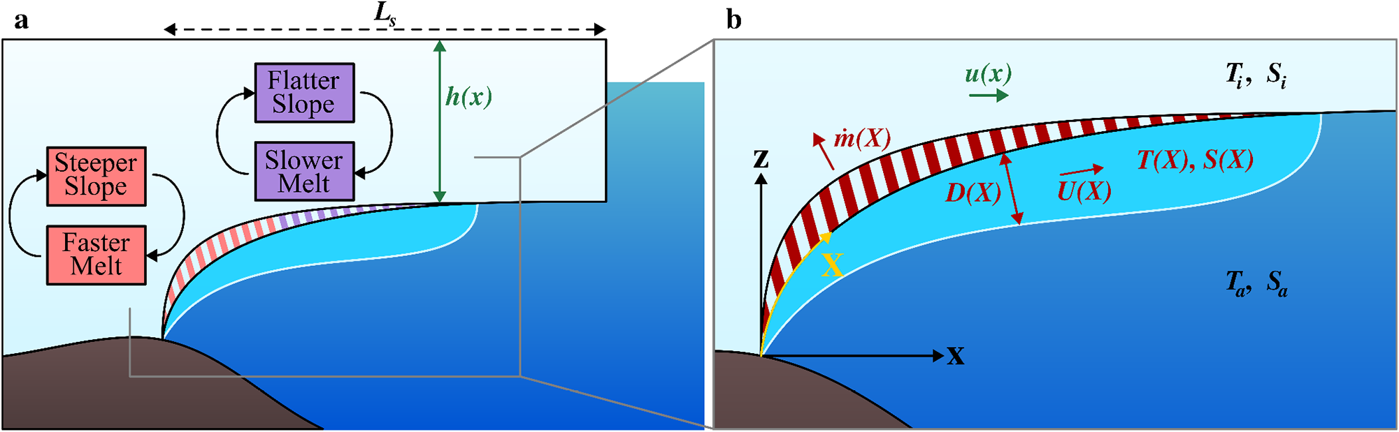
Here, we compare the performance of the local parameterization of Lazeroms and others (Reference Lazeroms, Jenkins, Rienstra and Van De Wal2019) with the plume model of Jenkins (Reference Jenkins2011) in a framework where the plumes are coupled to a dynamically evolving ice shelf, i.e., under conditions where the ice geometry is no longer assumed fixed but flows and responds to the intensity of the local melt rate. Since the ice shelf geometry evolves as a function of the melt rate, the changing shape of the ice shelf, in turn, modifies the melt rate itself. Specifically, the plume-induced melt rate is sensitive to the basal slope and the ice shelf draft, which leads to a positive feedback between basal melt and ice shelf geometry, as illustrated in Fig. 1a: large melting steepens the basal slope, which further enhances melting. Conversely, a lower melt rate results in a shallower slope, reducing the overall melt intensity. Our findings demonstrate that these feedbacks exacerbate the error between the local parameterization and the full plume system. Moreover, the use of the local parameterization leads to unrealistic discontinuities in the melt rate for a range of conditions.
Diagram of an ice shelf cavity with plume. Panel a illustrates the feedbacks that result from the direct coupling between the ice shelf geometry and plume-induced melting. Here,  $h(x)$ and
 $L_s$ are the ice shelf thickness and length. Panel b is a zoom-in on the plume region and shows the plume thickness
 $D(X)$, velocity
 $U(X)$, temperature
 $T(X)$ and salinity
 $S(X)$. Note the difference between the horizontal coordinate
 $x$ and the curvilinear coordinate
 $X$ (yellow), which follows the ice–ocean interface and evolves with time. The directions of ice and plume flow, and melt rate
 $\dot{m}(X)$ are illustrated with arrows. Also indicated are the ice shelf temperature
 $T_i$ and salinity
 $S_i$, as well as the ambient ocean temperature
 $T_a$ and salinity
 $S_a$.

The details of the model implementation are provided in Section 2, while readers primarily interested in the results may proceed directly to Section 3. Finally, in Section 4, we discuss the potential implications of our findings, as well as the broader applicability and limitations of the coupled model introduced here.
2. Model setup
2.1. Ice flow and geometry
We consider a confined ice shelf flowing in the positive  $x-$direction from the grounding line at
 $x=0$ to the terminus at
 $x_t$. The ice flow is modeled using the Shallow Shelf Approximation (SSA), which is widely employed to simulate ice shelf dynamics (e.g.,
MacAyeal, Reference MacAyeal1989; Dupont and Alley, Reference Dupont and Alley2005; Nick and others, Reference Nick, Vieli, Howat and Joughin2009; Hindmarsh, 2012; Pegler, Reference Pegler2016; Haseloff and Sergienko, Reference Haseloff and Sergienko2018; Reference Haseloff and Sergienko2022):
 \begin{equation}
\begin{aligned}
&\frac{\partial }{\partial x}\left(\frac{h}{A^{1/n}}\left|\frac{\partial u}{\partial x}\right|^{\frac{1}{n}-1}\frac{\partial u}{\partial x} \right) - \frac{C_W A^{-\frac{1}{n}}}{W^{\frac{1}{n}+1}}h\left|u\right|^{\frac{1}{n}-1}u \\
&= \frac{1}{2}\rho_i g \left(1-\frac{\rho_i}{\rho_w}\right)h\frac{\partial h}{\partial x},
\end{aligned}
\end{equation}
with  $h$ the ice thickness,
 $u$ the ice speed,
 $A$ the ice viscosity rate factor,
 $n$ the flow law exponent,
 $\rho_i$ the ice density,
 $\rho_w$ the seawater density,
 $g$ the acceleration due to gravity,
 $W$ the ice shelf width and
 $C_W$ a lateral shear stress parameter. Parameter values are given in Table A1 (Appendix A). The ice thickness evolution is determined from mass conservation:
 \begin{equation}
\frac{\partial h}{\partial t} + \frac{\partial }{\partial x}\left(uh\right) = -\dot{m},
\end{equation}
with  $\dot{m}$ the melt rate (positive for melting; negative for freeze-on).
At the grounding line, ice flux and ice thickness are prescribed:
 \begin{equation}
uh=q^{gl} \qquad \text{and } \qquad h=h^{gl} \qquad \text{at } x=0,
\end{equation}
where the superscript ‘gl’ signifies ‘grounding line’.
Stress balance is prescribed at the terminus, assuming a floating vertical ice front:
 \begin{equation}
\frac{2}{A^{1/n}}h\left|\frac{\partial u}{\partial x}\right|^{\frac{1}{n}-1}\frac{\partial u}{\partial x} = \frac{1}{2}\rho_i g \left(1-\frac{\rho_i}{\rho_w}\right)h^2 \qquad\mbox{at } x = x_t.
\end{equation}
The position of the terminus,  $x_t$, is determined by the melt rate: for low to moderate melt rates, it is fixed at
 $x_t=L_s$, but for sufficiently strong melt, the ice thickness can go to zero at
 $x_t \lt L_s$. The terminus position is indirectly determined as the first location where
 $h=0$:
 \begin{equation}
\begin{cases}
x_t=L_s \qquad &\text{if } h \gt 0 \,\forall \, x, \\
h(x_t)= 0 &\text{otherwise}.
\end{cases}
\end{equation}
2.2. Buoyant meltwater plume model
We assume that a buoyant meltwater plume drives circulation in the ice shelf cavity (illustrated in Fig. 1b), which sets the sub-shelf melt rate (Jenkins, Reference Jenkins1991; Reference Jenkins2011; Hewitt, Reference Hewitt2020). In this case, the basal melt rate is determined by the thermohaline difference between freshwater released from subglacial discharge and melted ice on the one hand and saline ocean water underneath the ice shelf on the other hand (Jenkins, Reference Jenkins2011). Generally, this leads to high melt rates close to the grounding line and possible refreezing further away. As discussed above, we compare two specific representations of this general plume model (Jenkins, Reference Jenkins2011; Lazeroms and others, Reference Lazeroms, Jenkins, Rienstra and Van De Wal2019):
2.2.1. Full plume model
We refer to the one-dimensional buoyancy-driven plume model from Jenkins (Reference Jenkins2011) as the ‘full plume model’. The model is described by conservation of mass (6a), momentum (6b), buoyancy (6c) and sensible heat (6d) within the plume:
 \begin{equation}
\frac{\partial }{\partial X}\left( D U\right) = \sin \alpha\, E_0 U + \dot{m},
\end{equation}
 \begin{equation}
\frac{\partial }{\partial X}\left( D U^2\right) = \sin \alpha\,gD \Delta\rho - C_dU^2,
\end{equation}
 \begin{equation}
\frac{\partial }{\partial X}\left( D U \Delta\rho \right) = \sin \alpha\,\frac{d\Delta\rho_a}{dz_b} DU + \dot{m}\Delta\rho_i^{ef},
\end{equation}
 \begin{align}
\frac{\partial }{\partial X}\left( D U \Delta T\right) =& \sin \alpha\,\left( T_a - T_{af} \right)E_0 U\\
& + \left( T_i^{ef} - T_{if}\right) \dot{m}- \sin \alpha\,\lambda_3 D U.\nonumber
\end{align}
 \begin{equation}
X = \int_0^x \sqrt{1+\left(\frac{\rho_i}{\rho_w}\frac{\partial h}{\partial x}\right)^2 } \text{d}x
\end{equation}
is the curvilinear coordinate along the shelf base,  $D$ the plume thickness,
 $U$ the plume velocity,
 $S$ the plume salinity and
 $T$ the plume temperature. The density difference between plume and ambient ocean is given by
 $\Delta\rho = \beta_S\left(S_a - S\right) - \beta_T\left(T_a - T\right)$, with
 $S_a$ and
 $T_a$ the ambient ocean salinity and temperature, and
 $\beta_S$ and
 $\beta_T$ the haline contraction and thermal expansion coefficients.
 $\Delta T = T - T_f$ is the temperature of the plume relative to its freezing temperature
 $T_f$. The ice shelf is in isostatic equilibrium, with the draft
 $z_b(x) = - h(x)\rho_i/\rho_w$. The local basal slope is
 \begin{equation}
\sin \alpha = -\frac{{\partial h}/{\partial x}}{\sqrt{(\rho_w/\rho_i)^2 + \left|{\partial h}/{\partial x}\right|^2}}.
\end{equation}
Furthermore, in Equation (6d),  $E_0$ is the plume entrainment coefficient,
 $C_d$ the drag coefficient,
 ${d\Delta\rho_a}/{dz_b}$ the slope of the ambient density contrast,
 $\Delta\rho_i^{ef}$ is the effective meltwater density contrast,
 $T_{af}$ is the ambient water freezing temperature,
 $T_{if}$ is the meltwater freezing temperature and
 $T_i^{ef}$ is the effective meltwater temperature (see Table A2 in Appendix A for expressions and parameter values).
The melt rate induced by the plume on the ice shelf  $\dot{m}$ is assumed to be directly proportional to the thermal forcing
 $\Delta T$ and the plume velocity
 $U$, such that
 \begin{equation}
\dot{m} = M_0 U \Delta T,
\end{equation}
where  $M_0$ is the melt rate factor (in
 $^{\circ}\mathrm{C}^{-1}$, see Table A2 in Appendix A).
At the grounding line, the plume is initiated by subglacial discharge. This discharge is assumed to be freshwater at freezing temperature, such that the initial conditions for the plume water are  $S^{gl} = 0$ psu and
 $T^{gl} = T_f^{gl}$. From this we determine
 $\Delta\rho^{gl}=\beta_SS_a - \beta_T\left(T_a - T_f^{gl}\right)$ and
 $\Delta T^{gl}= T^{gl} - T_f^{gl}=0$. The local plume representation defined below assumes no freshwater flux at the grounding line. For numerical stability, we introduce a small initial freshwater flux
 $DU^{gl} = 10^{-6}\;\text{m}^2 \text{s}^{-1}$ for full plume simulations. The plume thickness at the grounding line is arbitrarily set to
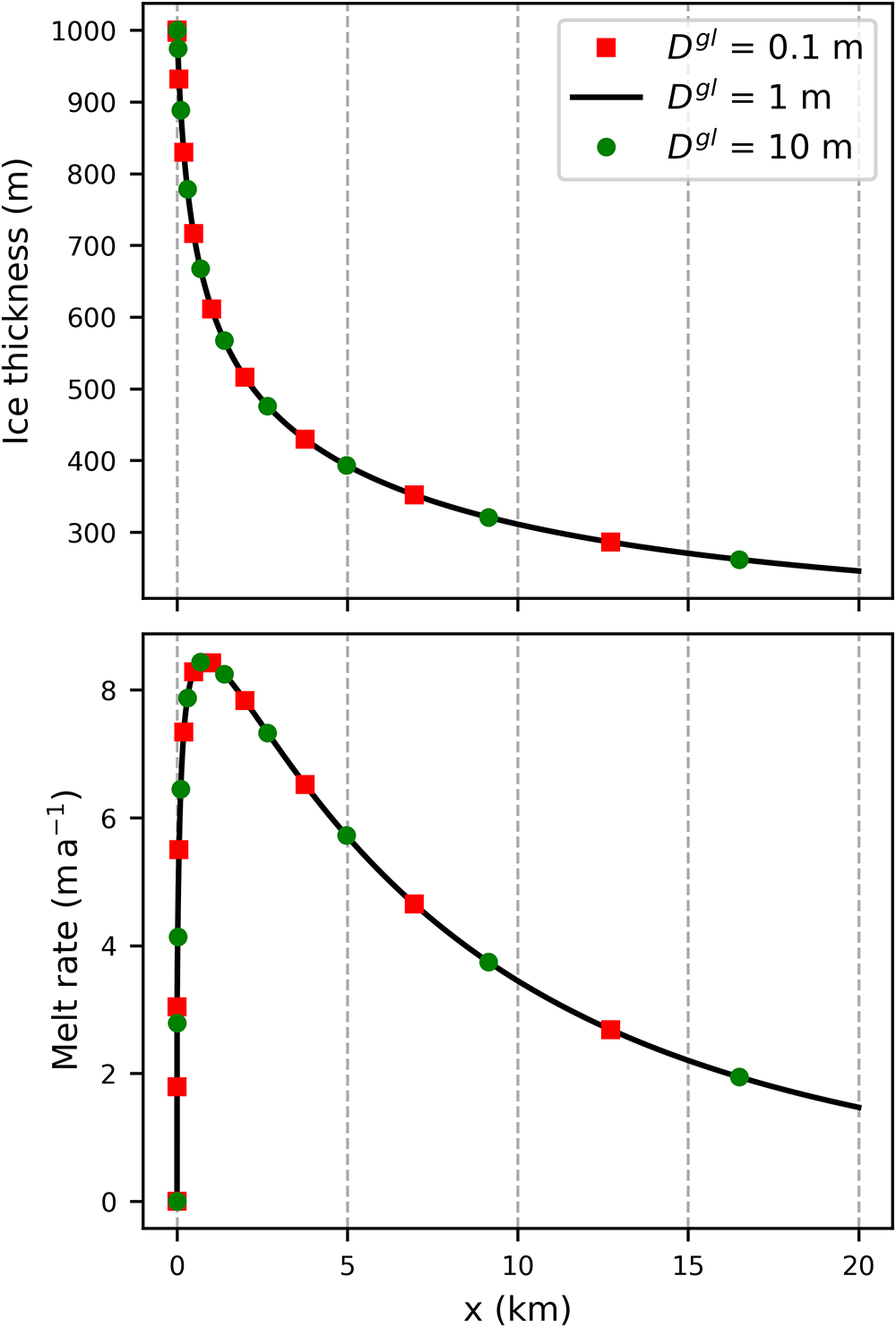
 $D^{gl} = 1 $ m. Varying
 $D^{gl}$ over three orders of magnitude indicates negligible impacts on the results (see Fig. B2 in Appendix B).
2.2.2. Local plume model
Lazeroms and others (Reference Lazeroms, Jenkins, Rienstra and Van De Wal2019) present a local approximation of plume-induced melting for constant and small basal slopes, based on asymptotic expansion and order of magnitude comparison. We will refer to this parameterization as the ‘local plume model’. In this model, the melt rate is determined from
 \begin{equation}
\begin{aligned}
\dot{m} = &\left(T_a - T_f^{gl}\right)^2 \mathcal{M}\left(\bar{x}\right)
\sqrt{\frac{\beta_S S_a g c^3}{\lambda_3 L^3} }\\
&\times \sqrt{\frac{1 - c_{\rho1}\Gamma}{C_d + E_0 \sin \alpha}}
\left(\frac{\Gamma E_0 \sin \alpha}{\Gamma + c_\tau + E_0\sin \alpha} \right)^{3/2},
\end{aligned}
\end{equation}
where  $\mathcal{M}(\zeta)$ is a non-dimensional melt function that varies with distance from the grounding line:
 \begin{equation}
\mathcal{M}\left(\zeta\right) = 2^{-3/2} \left[ 3\left(1-\zeta\right)^{4/3} -1 \right] \sqrt{1 - \left(1-\zeta\right)^{4/3}}.
\end{equation}
In Equation (10a),  $\bar{x}$ is the non-dimensional vertical distance from the grounding line depth with a slope-dependent correction factor:
 \begin{equation}
\bar{x} = \lambda_3\frac{z_b - z_b^{gl}}{T_a - T_f^{gl}}\left[1 + C_\epsilon\left( \frac{E_0 \sin \alpha}{\Gamma + c_\tau + E_0\sin \alpha}\right)^\frac{3}{4}\right]^{-1}
\end{equation}
Formally, the derivation of the local plume model assumes small, uniform basal slopes and uniform ocean conditions. However, it was found to compare well to the full plume model even when allowing for non-uniform basal slope and ocean conditions (Lazeroms and others, Reference Lazeroms, Jenkins, Rienstra and Van De Wal2019).
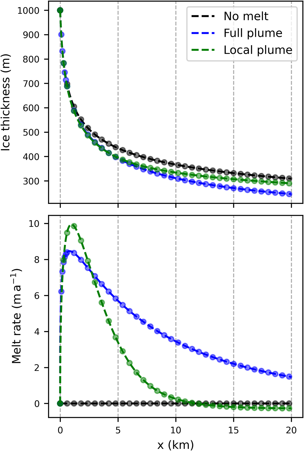
The steady-state ice shelf model (1)–(2) coupled either to the full plume (6a)–(9) or the local plume (10a)–(10c) can be reformulated as systems of first-order ordinary differential equations and are solved using the Python package SciPy’s integrate.solve_ivp (Virtanen and others, Reference Virtanen2020). The time-dependent system is solved with a finite-difference discretization using PETSc (Balay and others, Reference Balay2026). The steady-state solutions are compared to converged solutions of the PETSc integration in Fig. B1 for verification of the numerical methods (Appendix B).
3. Results
3.1. Plume model evaluation
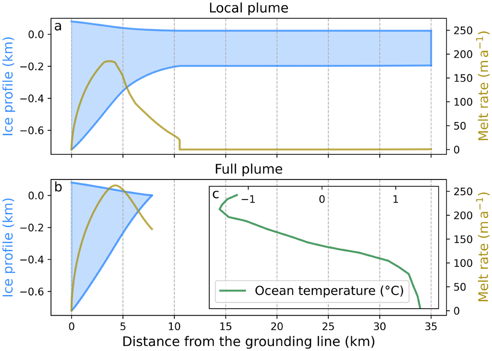
Ice profiles (blue) and melt rates (olive) for the steady-state solution of the coupled ice shelf–melt model with buttressing, for the local plume model in panel a and the full plume model in panel b. Here, ocean temperature is depth-varying (data from Burgard and others (Reference Burgard, Jourdain, Reese, Jenkins and Mathiot2022); shown in inset c, which has the same vertical axis as the main panel). See text for other simulation parameters and Appendix C for details on the temperature profile.

Figure 2 Long description
Panel A shows the ice shelf thickness and basal melt profiles for the local plume simulation. The ice shelf becomes nearly flat after about 10 kilometers, while the basal melt rate decreases to zero. Panel B shows the corresponding profiles for a full plume simulation, in which stronger basal melting causes the ice shelf to terminate much closer to the grounding line. Panel C shows the ocean temperature profile used in both simulations, with temperatures increasing from about –1 °C near the surface to about 1 °C near the seabed.
Our results indicate that for a range of conditions, the local plume model leads to unphysical behavior once it is coupled to an evolving ice shelf. Fig. 2a shows a representative solution for a steady-state ice shelf with Thwaites Ice Shelf-like conditions: the grounding line thickness is  $h^{gl} = 800$ m, the initial ice velocity is
 $ u^{gl} = 2000\, \text{m}\,\text{a}^{-1}$, the width of the shelf is
 $W = 80$ km and the ambient ocean temperature
 $T_a$ depends on the depth and is extracted from Burgard and others (Reference Burgard, Jourdain, Reese, Jenkins and Mathiot2022) (see Appendix C for details). In this scenario, the melt rate shows a discontinuity (or jump) to
 $\dot{m} = 0$ at
 $x_d = 10.5$ km. This leads to a uniform ice thickness
 $h\left(x \gt x_d\right)$ and beyond that point the melt is zero or small (but always positive). Conversely, the full plume (6a)–(9) leads to ice shelf melting and thinning until it reaches zero thickness at
 $x_t = 7.8$ km (Fig. 2b).
Figure 2 illustrates the discontinuity in a simulation that includes buttressing effects, in addition to the variable ocean temperature profile. As we discuss below in Section 4, buttressing and ocean temperature variations do not cause the melt discontinuity. We therefore neglect buttressing (by formally assuming  $W \rightarrow \infty$ in Eq. (1)) and assume a uniform ocean temperature from here on.
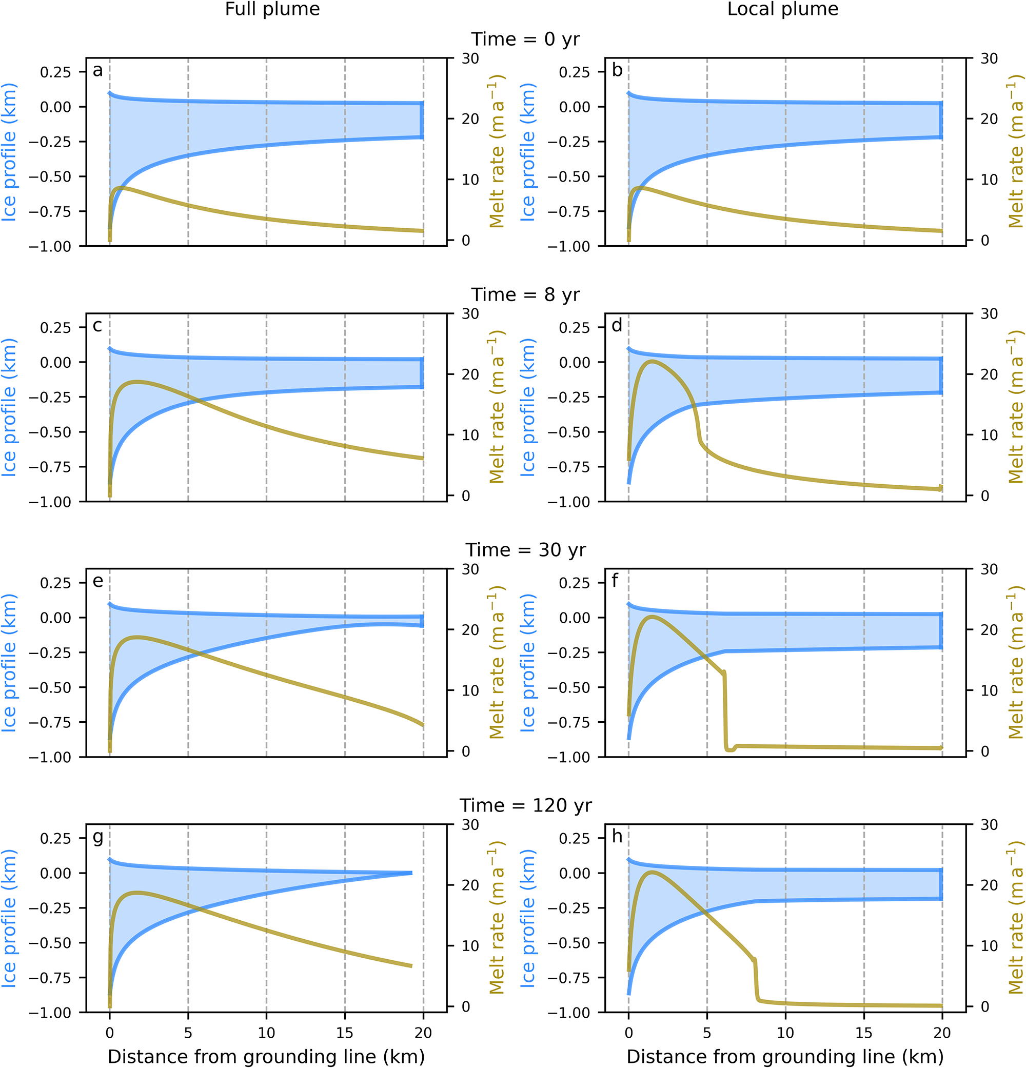
Snapshots of the time-dependent solution of the coupled ice shelf–melt model. The ice shelf profiles (blue) and melt rates (olive) are shown for both the full plume model (left column) and the local plume model (right column). Solutions are shown at  $t = 0,\, 8,\, 30$ and 120 years. The grounding line thickness is
 $h^{gl} = 1000$ m, the initial ice velocity is
 $ u^{gl} = 250$
 $\text{m}\,\text{a}^{-1}$ and the ambient ocean temperature is
 $T_a = -1.6^{\circ}$C. The initial state in panels a and b is given by the steady-state solution of the coupled full plume model with an ocean temperature
 $T_a = -1.9^{\circ}$C.

To confirm that the results shown in Fig. 2 are not due to a numerical instability or the assumption of steady-state, we consider the time-dependent system (solved using PETSc). The initial state is obtained from a prior simulation of the coupled full plume model run to steady-state at an ocean temperature of  $T_a = -1.9^{\circ}$C. Both the full plume PETSc simulation and the local plume PETSc simulation are initialized with this ice shelf (Fig. 3a and b, respectively). The ocean temperature is increased to
 $T_a = -1.6^{\circ}$C and the model is integrated to a new steady state for both the full plume (left column of Fig. 3) and the local plume (right column). For the local plume model, a small perturbation in the otherwise smooth melt emerges at the grounding line and propagates downshelf shortly after initialization (see
 $x = 4$ km in Fig. 3d). The perturbation continues to propagate and grow, and a discontinuity appears at
 $x = 6$ km as shown in Fig. 3f. The discontinuity then sharpens and propagates until it becomes stationary at
 $x = 8$ km (Fig. 3h). This unphysical behavior is known as a shock (e.g.,
Fowler, Reference Fowler1997). Conversely, in the full plume model, melt is continuous along the full extent of the ice shelf and the ice shelf front melts completely by the end of the simulation, with the front retreating to
 $x_t = 19$ km (Fig. 3g).
3.2. Origin of the melt discontinuity
The highly nonlinear dependence of the melt rate on ice shelf slope  $\sin\alpha$ and thickness
 $h$ prevents a closed-form analytical solution, but we can qualitatively understand the problematic behavior. Momentarily neglecting the slope-dependent correction factor in Equation (10c), the local plume melt rate depends on basal slope as:
 \begin{equation}
\dot{m} \,\propto\, \sqrt{\frac{1 - c_{\rho1}\Gamma}{C_d + E_0 \sin \alpha}}
\left(\frac{\Gamma E_0 \sin \alpha}{\Gamma + c_\tau + E_0\sin \alpha} \right)^{3/2}.
\end{equation}
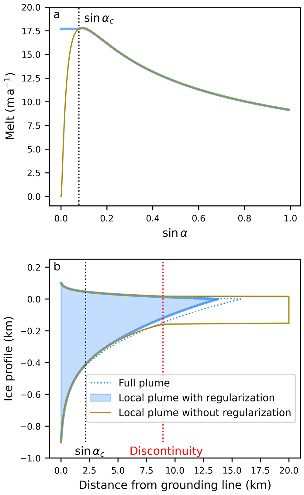
The qualitative behavior is shown in Fig. 4a (olive line).
Importantly,  $\dot m\rightarrow 0$ for
 $\sin\alpha\,\propto\,\partial h/\partial x \rightarrow 0$. To see why this is problematic, we can integrate the momentum balance Equation (1) with
 $W\rightarrow\infty$ by use of the boundary condition at the calving front (4) to obtain (e.g.,
Schoof, Reference Schoof2007)
 \begin{equation}
\frac{h}{A^{1/n}}\left|\frac{\partial u}{\partial x}\right|^{\frac{1}{n}-1}\frac{\partial u}{\partial x} = \rho_i g \left(1-\frac{\rho_i}{\rho_w}\right)h^2.
\end{equation}
Introducing the flux  $q=uh$ and rearranging gives
 \begin{equation}
\frac{1}{h}\frac{\partial q}{\partial x} - \frac{q}{h^2}\frac{\partial h}{\partial x} = A \left[\rho_i g \left(1-\frac{\rho_i}{\rho_w}\right)\right]^n h^{n},
\end{equation}
 \begin{equation}
\frac{\partial q}{\partial x} = \dot m,
\end{equation}
 $h \gt 0$. Assuming this is the case, we can see that in the limit of
 $\partial h/ \partial x=0$, the first Equation (13a) requires
 $h=0$ for
 $\partial h/ \partial x = \partial q/ \partial x = 0$ when
 $\dot m(\partial h/ \partial x=0) =0$. Since
 $h \gt 0$ and
 $h=0$ cannot be satisfied simultaneously, unphysical behavior ensues. Physically, this means that when the ice thickness and flux simultaneously become constant, mass balance requires the velocity to be constant too (as
 $q=uh$). However, the momentum balance requires the velocity to linearly increase for constant, non-zero ice thicknesses in order to satisfy the force balance at the calving front. This latter behavior can be seen in the velocity solutions past the discontinuity (not shown).
The earlier 11-term plume parameterization by Lazeroms and others (Reference Lazeroms, Jenkins, Gudmundsson and van de Wal2018) prescribes the same dependence on ice shelf slope and consequently shows the same discontinuity (see Fig. B3 in Appendix B and Discussion). Conversely, in the full plume model a zero slope does not automatically require  $\dot m\rightarrow 0$, and the problem does not arise.
3.3. Regularization of the melt discontinuity
We can further show that the problematic behavior is linked to the limiting behavior of  $\dot m(\partial h/\partial x \rightarrow 0)$ by regularizing the melt rate so that
 $\dot m(\partial h/ \partial x \rightarrow 0)\neq 0$. The simplest such regularization replaces the slope used in the melt equation so that it does not fall below a prescribed threshold:
 \begin{equation}
\sin\alpha' = \max\left(\sin\alpha,\; \sin\alpha_c\right).
\end{equation}
Here, we choose the threshold  $\sin \alpha_c$ that maximizes the melt rate
 $\dot{m}$ for small slopes. This can be determined analytically from Equation (10a) when the slope-dependent correction factor is neglected:
 \begin{equation}
\sin\alpha_c = \frac{\Gamma + c_\tau}{E_0}\left(1 + \sqrt{1+3\frac{C_d}{\Gamma + c_\tau}}\right).
\end{equation}
This simple regularization effectively prevents the discontinuity described above (Fig. 4b) without significantly affecting other parameter ranges (not shown). By limiting the slope within the melt function, the late-stage behavior of the plume (melt/refreezing) is preserved in most cases, while the sudden melt discontinuity is avoided (Fig. 4a).
Example of the regularized melt (solid blue) compared to the default local plume parameterization (olive). Panel a illustrates the melt rate as a function of the slope ( $\sin\alpha$) at the location of the discontinuity (dotted red line in panel b), while panel b shows the ice thickness profile with the full plume solution in dotted blue.

Figure 4 Long description
Two-panel figure comparing three basal melt parameterizations: the full plume model, the local plume model, and the local plume model with regularization. Panel A shows the dependence of basal melt on ice-shelf slope, with and without regularization. Panel B shows the resulting ice shelf thickness profiles. The regularized local plume profile closely matches the full plume profile, whereas the unregularized local plume produces an unrealistically flat ice shelf.
3.4. Plume parameterization impact on melting
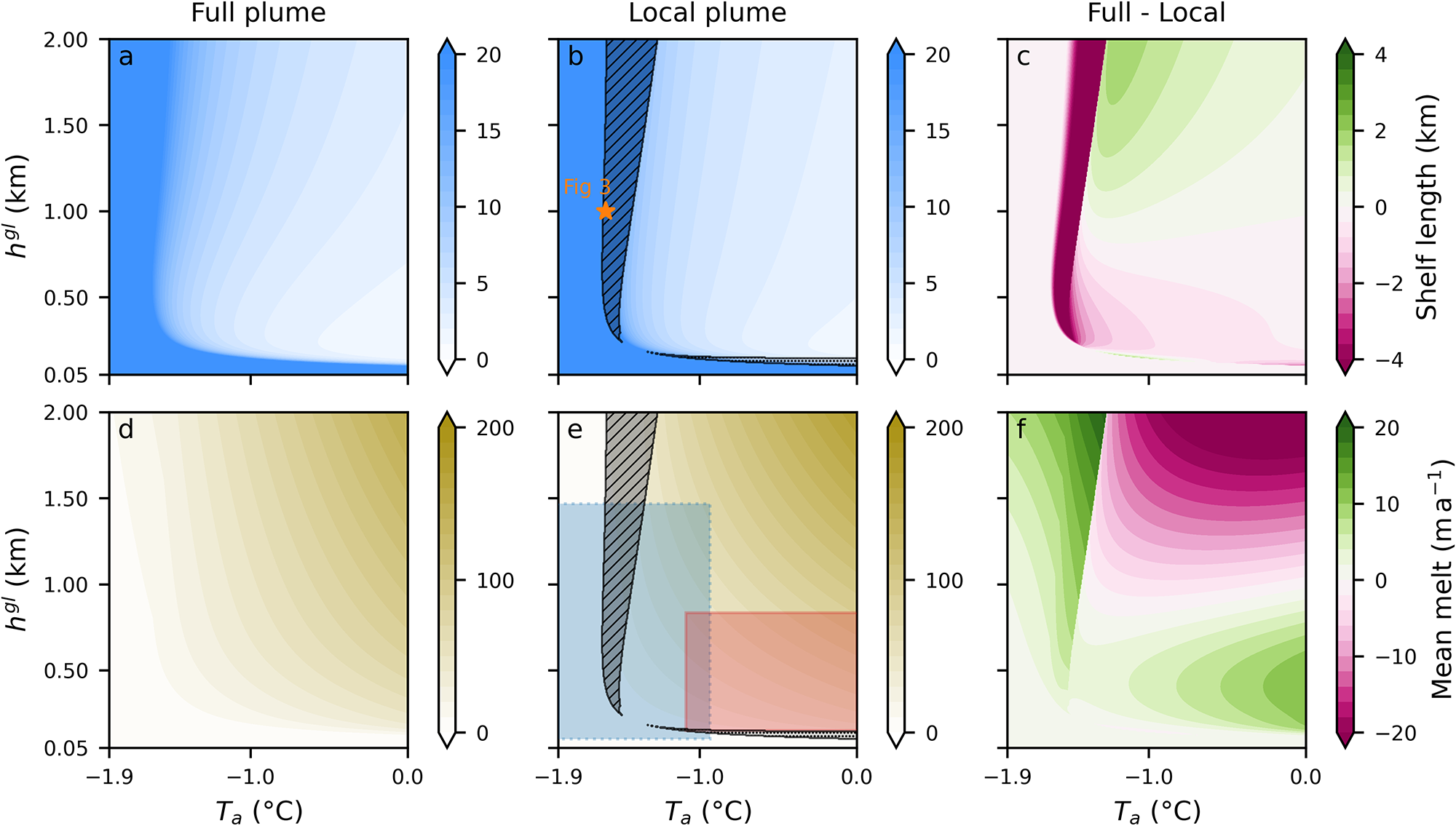
To identify the range of solutions that feature the unphysical behavior described above, we compare steady-state solutions of the full plume model to those of the local plume model over a wide range of parameters. We focus on varying the grounding line thickness ( $h^{gl}$) and the uniform ambient ocean temperature (
 $T_a$). Here, we consider the dependence of two ice shelf properties on these parameters: ice shelf length
 $L_s$ (top row in Fig. 5) and mean melt rate (bottom row in Fig. 5)—which can be estimated from the ice flux difference as:
 $\frac{1}{x_t}\int_0^{x_t}\dot{m} \text{d}x = \left[q^{gl} - q\left(x_t\right)\right]/x_t$.
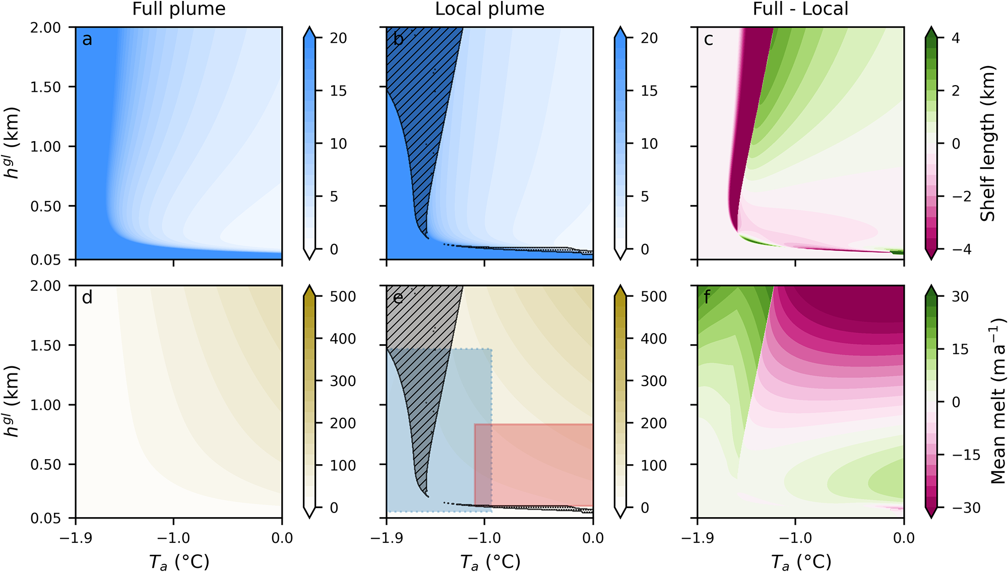
The hatched regions in Fig. 5b and e delineate areas where discontinuities in the melt rate occur. These discontinuities appear in two distinct branches, corresponding to the two melt–slope feedback mechanisms illustrated in Fig. 1a. The melt–slope feedbacks are a physical feature of the system and act in both the full and local plume models. However, the feedbacks only manifest as discontinuities in the local plume model.
The roughly vertical branch, occurring at temperatures between  $-1.6^\circ$C and
 $-1.1^\circ$C, corresponds to the instability discussed above due to a feedback of shallower slopes leading to less melt and less viscous thinning. In this regime, the discrepancies between the local and full plume models are substantial: the ice-shelf length is overestimated by up to approximately 9 km (90 % relative error), and the mean melt rate is underestimated by up to
 $20\;\text{m}\,\text{a}^{-1}$ (50 % relative error).
The horizontal branch, characterized by initial ice thicknesses ranging from 80 to 150 m and exhibiting little sensitivity to ocean temperature, originates from this feedback operating in reverse with steeper slopes leading to more melt. In this parameter regime, the feedback induces rapid thinning at the ice front (not shown). This positive feedback was previously identified in a coupled modeling framework by Haseloff and Sergienko (Reference Haseloff and Sergienko2022), using a simplified plume parameterization. Our results suggest that this behavior is not an artifact of their simplified framework but rather a physical process and an intrinsic feature of plume-based parameterizations in the limit of steep slopes, which can emerge under realistic ice-shelf conditions. For the full plume model, the steep-slope feedback also results in an abruptly terminating ice shelf, but without introducing a discontinuity in the melt rate. Relative to the full plume model, the length differs by  $\pm$2 km (up to 30 % relative error) and the mean melt rate is up to
 $6\;\text{m}\,\text{a}^{-1}$ less (30 % relative error).
For the remainder of this study, we focus on the shallow-slope feedback regime, since despite inducing some discrepancies in the predicted melt rates and ice-shelf length, the overall physical behavior remains consistent between the local and full plume models in the steep-slope regime.
Outside of the discontinuity regimes, we find that in the coupled system, the local plume introduces errors of up to  $\pm$ 2 km (30 % relative error) in the predicted shelf length (Fig. 5c). The average melt rates differ by up to
 $\pm$ 20
 $\text{m}\,\text{a}^{-1}$ depending on the conditions, which corresponds to a relative error of 20 to 30 %. For cold ocean temperatures (
 $ \lt -1.8^\circ$C), the relative error between the full and local plume formulations can reach 80%. The error in melt is partially obscured when considering average melt rates, as the mean smooths out discrepancies between the two models. Specifically, the local plume tends to overestimate melt near the grounding line and underestimate it farther downstream, resulting in partial compensation of local melt-rate errors.
Sensitivity of the coupled model to changes in ambient ocean temperature  $T_a$ and initial ice thickness
 $h^{gl}$. Each simulation is performed for both the full plume model (left column) and the local plume model (middle column), with the difference shown in the right column. The first row shows contours of ice shelf length, and the second row shows contours of average melt rates. The hatched areas in panels b and e show regions of discontinuity in the melt rate. The two boxes in panel e broadly indicate the relevant parameter space for ice shelves around Antarctica: blue with dashed outline for cold cavities, and red with solid outline for warm cavities (Appendix C provides details on the calculation and data used for the box extents). The orange star in panel b marks the examples shown in Figure 3.

Figure 5 Long description
Six-panel figure arranged in two rows and three columns. All panels share the same axes: ocean temperature on the x-axis and initial ice thickness on the y-axis. The top row shows ice shelf length, and the bottom row shows mean basal melt rate. The left column presents results from the full plume model, the middle column presents results from the local plume model, and the right column shows the difference between the two models.
4. Discussion
The unphysical behavior of local plume parameterizations in a coupled setting has—to our knowledge—not been previously reported, even though the coupled setting has been used in several previous studies (Favier and others, Reference Favier2019; Berends and others, Reference Berends, Stap and van de Wal2023; Coulon and others, Reference Coulon, De Rydt, Gregov, Qin and Pattyn2024a). We hypothesize that this omission is due to the subtle nature of the instability, which makes it hard to detect in models with complex ice shelf geometries and coarser resolution. Moreover, a continuously evolving grounding line, ice influx or oceanic conditions may mute its effects or prevent its emergence altogether.
The unphysical behavior of the local plume melt observed above arises from its coupling with ice dynamics. Near the grounding line, both the melt rate and the basal slope are large, and the local plume model performs relatively well compared to the full plume model. Further away from the grounding line, the ice shelf flattens because of viscous thinning, leading to a reduction in melt. Under cold ambient ocean temperatures ( $\sim -1.9^{\circ}$C) and small basal slopes, the melt rate varies smoothly, resulting in a gradual transition to flatter ice shelves. However, the melt rate sensitivity to changes in basal slope—and hence the feedback between ice geometry and melt—increases with ambient ocean temperature. This leads to the abrupt decrease in slope and melt at relatively warmer temperatures (
 $\sim -1.5^{\circ}$C) in the local plume model. For a range of temperatures and grounding line thicknesses, this transition becomes so sharp that it manifests as a sudden discontinuity in both melt rate and slope. The finding that the polynomial parameterization from Lazeroms and others (Reference Lazeroms, Jenkins, Gudmundsson and van de Wal2018), exhibits the same type of instability (cf. Fig. B3 in Appendix B) supports our conclusion that the instability results from the locality of the parameterization.
The nonlinear dependence of the melt rate on ice shelf slope  $\sin\alpha$ and thickness
 $h$ prevents a closed-form analytical solution of the model. However, we can qualitatively understand its emergence by considering the limit of
 $\partial h/\partial x\rightarrow0$, as discussed in Section 3.2. In the local melt rate parameterizations, there is no melt at vanishing ice shelf slopes, requiring a constant ice shelf flux, and hence ice velocity in steady state. For non-zero ice thicknesses, this violates the momentum balance equation, which requires an increasing ice velocity in the downstream direction for constant ice thicknesses. Notably, the condition of vanishing melt at vanishing basal slope is present in both local formulations (Lazeroms and others, Reference Lazeroms, Jenkins, Gudmundsson and van de Wal2018; Reference Lazeroms, Jenkins, Rienstra and Van De Wal2019), which explains why both parameterizations exhibit the same discontinuity behavior.
4.1. Relevance for realistic ice shelf studies
To assess the relevance of the instability for real ice shelves, we consider representative values for  $h^{gl}$ and
 $T_a$ for both cold and warm ice shelves, which are indicated in Fig. 5e by the blue and red bounding boxes, respectively. To determine these ranges, we used the annual mean ocean temperature between 200 m below sea level and the sea bed in front of 18 Antarctic ice shelves from the World Ocean Atlas 2023 (Reagan and others, Reference Reagan2024). The grounding line thickness was estimated by averaging the ice thickness over a 4 km wide strip centered around the grounding line. We used the BedMap3 dataset for both ice thickness and grounding line position (Pritchard and others, 2025). The two temperature regimes were then identified based on the clustering of ocean temperature. The ‘cold’ regime comprises the Ross, Mertz, Totten, Shackleton, Amery, Filchner, Ronne, Larsen and Dotson ice shelves (blue box,
 $T_a\in\lbrack-1.9,$
 $-0.9]^{\circ}$C), whereas the ‘warm’ regime includes the Rennick, Cook, Baudouin, Stancomb-Brunt, Wilkins, Abbot, Getz, Pine Island and Fimbul ice shelves (red box,
 $T_a\in\lbrack-1.1,0.5\rbrack^\circ$C). Further details regarding the classification method and the data used are provided in Appendix C. The ‘cold’ box largely contains the region of instability (hatched area), indicating that this issue is applicable to relevant ice shelf environments. Aside from the instability, the parameterization induces a relative melt rate error of -80% to 25% for cold ice shelves, depending on the initial condition. In contrast, the ‘warm’ box barely overlaps with the hatched area, but some of the warm shelves also encounter substantial melt bias (underestimations of 10%–30%), in particular since the boxes represent standard deviations around mean values, not the minimum/maximum values of
 $h^{gl}$ and
 $T_a$.
4.2. Study limitations
The results presented above are derived from a highly idealized framework. This allows us to understand and evaluate the performance of different melt rate parameterizations, but we omit several processes that may limit the extension of our results to more complex conditions. The most substantial limitation of our study may be the use of a 1D-flowline model. Realistic ice shelf geometries are complex and deviate significantly from the channel flow assumed here. When considering two horizontal dimensions, the local plume parameterization would still require a vanishing steady-state flux divergence for flat ice shelves. However, it is not immediately obvious what the dynamic consequences of this requirement are. Our results in Fig. 2 illustrate that buttressing by itself is not sufficient to mitigate the melt discontinuity, and future work should investigate the consequences of the local parameterization to verify that it does not lead to unintended melt artifacts which might be obscured by the complexity of the problem.
The one-dimensional nature of the model also assumes alignment of plume and ice flow. In reality, this assumption is unlikely to hold: the plume trajectory is influenced by variations in basal topography, the Coriolis force deflects plumes over long distances, and external forcings such as sub-shelf circulation and tides can significantly modify the plume path. Nevertheless, we consider our findings to remain relevant for two main reasons: i) The one-dimensional limitation is not unique to the local parameterization but is inherent to the original full plume model. Thus, the framework adopted here is consistent with the assumptions under which the local parameterization was originally derived, and a proper two-dimensional extension remains an important but separate future effort. ii) The local parameterization has been proposed (Lazeroms and others, Reference Lazeroms, Jenkins, Rienstra and Van De Wal2019) as a two-dimensional melt parameterization applicable across ice-shelf cavities without explicit representation of the plume along flow paths. It is reasonable to expect that limitations identified in the one-dimensional setting provide a useful indicator of the potential issues in a two-dimensional context.
For the majority of this study, we neglected ocean temperature stratification. While important for a more realistic depiction of ice shelf dynamics, our results in Fig. 2 indicate that this simplification does not prevent the occurrence of the identified discontinuity.
We also assume that the ice is at a constant temperature of  $T=0^{\circ}$C. In reality, ice shelves exhibit a temperature gradient, with a colder surface and a relatively warmer base, resulting in variations in ice stiffness. This influences both the melt rate and the plume’s development through two primary mechanisms: (i) the impact on ice dynamics and (ii) the sensible heat required to warm the ice near the interface and bring it to the melting point. The latter has a minimal effect on melting and was shown to be negligible in the local plume parameterization by Lazeroms and others (Reference Lazeroms, Jenkins, Rienstra and Van De Wal2019). However, regarding (i), Sergienko and others (Reference Sergienko, Goldberg and Little2013) showed that the changes in stiffness can induce important changes in geometry and thus melt, with differences up to 20% in the case of warm cavities.
The proposed regularization of the local plume model introduces only minor discrepancies with the full plume model in our non-buttressed, flow-line ice-shelf framework. However, real ice shelves experiencing significant buttressing typically exhibit smaller basal slopes at the grounding line than those predicted by our model. Consequently, the proposed regularization may not be appropriate for such ice shelves, as it would lead to an overestimation of melt rates. The regularization introduced here should be interpreted primarily as confirmation that the underlying issue has been correctly identified, rather than as a definitive correction of the local plume model.
The model employed here does not include a calving parameterization, which explains the unrealistic scenario of the shelf gradually reaching  $h = 0$ at
 $x = x_t$. In reality, an ice shelf would likely calve once its thickness falls below a certain threshold or when some stress criterion is passed (e.g.,
van der Veen, Reference van der Veen1998; Benn and others, Reference Benn, Hulton and Mottram2007; Nick and others, Reference Nick, van der Veen, Vieli and Benn2010; Choi and others, Reference Choi, Morlighem, Rignot and Wood2021). However, the discussion in Section 3.2 is independent of the calving law, so that the behavior reported here remains relevant with the inclusion of a calving law, in particular when calving is not triggered before the melt discontinuity occurs.
Finally, it is worth noting that plume parameterizations are not the only viable approach for representing basal melting beneath ice shelves, with several studies having explored a range of avenues that could serve as an alternative to the local plume parameterization, in particular if the issues identified here prove significant in two dimensions (Reese and others, Reference Reese, Albrecht, Mengel, Asay-Davis and Winkelmann2018; Favier and others, Reference Favier2019; Burgard and others, Reference Burgard, Jourdain, Reese, Jenkins and Mathiot2022; Berends and others, Reference Berends, Stap and van de Wal2023; Coulon and others, Reference Coulon, De Rydt, Gregov, Qin and Pattyn2024a).
5. Conclusion
The gravity-driven circulation in ice shelf cavities is believed to be a key cause of basal melting. Yet, high complexity and computational cost prevent full cavity simulations in climate models for long timescales or for large ensembles. Standalone ice sheet models require melt parameterizations to incorporate ocean simulations and improve boundary representation (Levermann and others, Reference Levermann2020; Seroussi and others, Reference Seroussi2020). Consequently, sub-shelf melt must be parameterized in both modeling frameworks. In this study, we explored one basal melt rate parameterization—proposed by Lazeroms and others (Reference Lazeroms, Jenkins, Rienstra and Van De Wal2019)—which simplifies the full plume parameterization from Jenkins (Reference Jenkins2011) to a local approximation. This parameterization has previously been validated for fixed ice shelf configurations only, i.e., without accounting for feedback between the computed melt rate and the evolving basal profile (e.g., Burgard and others, Reference Burgard, Jourdain, Reese, Jenkins and Mathiot2022). To assess the robustness of the local parameterization, we developed a dynamically coupled model that integrates ice shelf evolution and plume-induced melt rates. We report that under certain conditions of ambient ocean temperature and grounding line ice thickness, the local melt rate parameterization exhibits unphysical behavior as it does not allow mass and momentum balances to be satisfied simultaneously. This anomaly results in melt rate discontinuities and in the prediction of unphysically long and thick ice shelves.
The range of ambient ocean temperatures for which the discontinuity is observed is around  $-1.6^{\circ}\mathrm{C}$ to
 $-1.1^{\circ}\mathrm{C}$ for grounding line ice thicknesses larger than
 $\sim 200$ m, which is in the range found near a number of Antarctic ice shelves. Outside this parameter space, the coupling induces greater discrepancy than in a fixed model: the mean melt rate can show a difference of
 $\pm$ 20
 $\mbox{m}\,\mbox{a}^{-1}$ relative to the full plume model, with a tendency to underestimate melt rates in the parameter range relevant for Antarctic ice shelves. We conclude that unintended artifacts can arise when coupling ice sheet dynamics to melt processes. Future work should evaluate these effects and feedbacks of local melt rate parameterizations in a two-dimensional coupled framework.
Acknowledgements
N.B.S. and T.J.W.W. were supported by the NSF Office of Polar Programs through grants # 2148544 and # 2338057. M.H. acknowledges NSF grant # 2218463. This research was supported in part by grant NSF PHY-2309135 to the Kavli Institute for Theoretical Physics (KITP). Finally, we thank the reviewers for their thorough and thoughtful feedback.
Appendix A
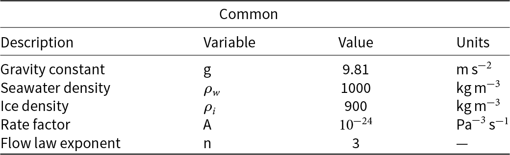
Parameters from the shallow shelf model and the plume models as described in the text.

Table A1 Long description
Common physical and rheological constants used in the shallow shelf and plume modeling are listed with their values and units. Gravity is 9.81 meters per second squared. Seawater density is 1000 kilograms per cubic meter, while ice density is 900 kilograms per cubic meter, so seawater is 100 kilograms per cubic meter denser than ice. The ice flow rate factor is 10 to the minus 24 in units of pascal to the minus three per second, indicating a very small coefficient in the flow relation. The flow law exponent is 3 and is unitless. Values are presented as fixed constants and do not indicate variability or uncertainty ranges.
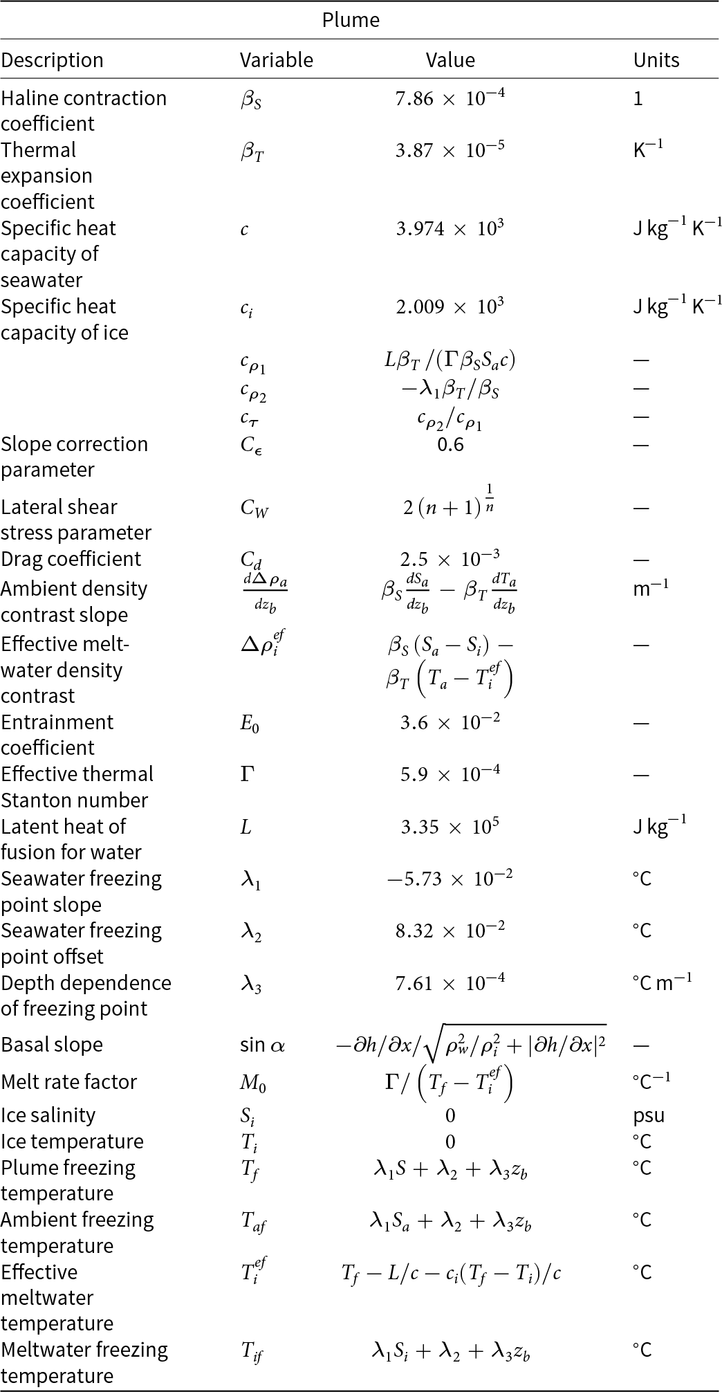
Parameters and variables of the plume models as described in the text. Following Jenkins (Reference Jenkins2011), we replace  $T_f$ with
 $T_{af}$ in the expressions of
 $M_0$ and
 $T_i^{ef}$ in our simulations, which simplifies the numerical integration and has no measurable impact on the results.

Table A2 Long description
Plume-model parameters and variables are listed with names, symbols, numerical values or definitions, and units. Physical constants include haline contraction and thermal expansion coefficients, seawater and ice heat capacities, and latent heat of fusion. Model tuning parameters include a slope correction value of 0.6, a drag coefficient of 0.0025, and an entrainment coefficient of 0.036, plus a lateral shear stress parameter defined from an exponent. Several entries define density-contrast terms: one for the ambient vertical gradient and another for effective meltwater density contrast, both described using salinity and temperature differences and their sensitivities. Freezing-related variables include plume freezing temperature, ambient freezing temperature, meltwater freezing temperature, and an effective meltwater temperature, each expressed as functions of salinity and depth with stated units in degrees Celsius. Ice properties are set to zero salinity and zero temperature. Some rows provide dimensionless derived coefficients and a melt-rate factor defined from a heat-transfer number and a temperature difference, so values may depend on other variables rather than being fixed numbers.
Appendix B
Steady-state ice profiles (top) and melt rates (bottom) calculated using Python (dashed lines) and PETSc (dots) for ambient ocean temperature  $T_a = -1.9^{\circ}\mathrm{C}$. Three different melt parameterizations are shown: no melt (black), the local plume model (green) and the full plume model (blue).

Influence of the initial plume thickness  $D^{gl}$ on the coupled system with the full plume model:
 $D^{gl} = 0.1$ m (red),
 $D^{gl} = 1$ m (black) and
 $D^{gl} = 10$ m (green). The ambient ocean temperature is
 $T_a = -1.9^{\circ}\mathrm{C}$. Note that the results are not sensitive to a change in
 $D^{gl}$ across three orders of magnitude.

Identical to Figure 5 but with the plume parameterization from Lazeroms and others (Reference Lazeroms, Jenkins, Gudmundsson and van de Wal2018) instead of that from Lazeroms and others (Reference Lazeroms, Jenkins, Rienstra and Van De Wal2019).

Figure B3 Long description
Six-panel figure arranged in two rows and three columns. All panels share the same axes: ocean temperature on the x-axis and initial ice thickness on the y-axis. The top row shows ice shelf length, and the bottom row shows mean basal melt rate. The left column presents results from the full plume model, the middle column presents results from the local plume model, and the right column shows the difference between the two models.
Appendix C
We selected 18 ice shelves to broadly represent the conditions at the base of Antarctic ice shelves. The selection was made to ensure a geographically representative distribution around Antarctica while focusing on the larger ice shelves. The two boxes shown in Fig. 5 were derived using QGIS (QGIS Development Team, 2025) as described below.
Ocean temperatures were obtained from the World Ocean Atlas 2023 dataset for both winter and summer (Reagan and others, Reference Reagan2024), with one exception for Pine Island, where we used the ocean temperature data from Burgard and others (Reference Burgard, Jourdain, Reese, Jenkins and Mathiot2022) since the World Ocean Atlas 2023 missed data. Each ice shelf was manually delineated, with the masking region extending a few grid cells in front of the shelves. The temperature was averaged both spatially across each shelf from the sea bed to 200 m below sea level, and temporally across summer and winter. The 200 m depth temperature was selected as a representative proxy for potential warm water intrusions into the ice shelf cavities. The separation of shelves into two groups was solely based on the temperature because it creates a clear distinction with a threshold at  $-1^{\circ}\mathrm{C}$. The ‘cold’ regime comprises the Ross, Mertz, Totten, Shackleton, Amery, Filchner, Ronne, Larsen and Dotson ice shelves (blue box,
 $T_a = [-1.9,$
 $-0.9]^{\circ}\mathrm{C}$). These shelves are located farther south and further from the continental shelf edge than other ice shelves, thereby remaining isolated from the Antarctic Circumpolar Current. In contrast, the ‘warm’ regime includes the Rennick, Cook, Baudouin, Stancomb-Brunt, Wilkins, Abbot, Getz, Pine Island and Fimbul ice shelves (red box,
 $T_a = [-1.1, 0.5]^{\circ}\mathrm{C}$), which are closer to the continental shelf break, more exposed to warmer water and subject to higher levels of basal melting.
The grounding line position and ice thickness were obtained from Bedmap3 (Pritchard and others, 2025). To account for uncertainties related to grounding zone migration, the entire grounding line was buffered by 2 km. For each ice shelf, the grounding line was segmented into distinct polygons. Ice thickness statistics were derived for each grounding zone polygon separately (grouped by ice shelf), excluding grid points with zero ice thickness. Finally, the boundaries of each box in Fig. 5 are defined as the extrema of the mean  $\pm$ one standard deviation for each ice shelf.
The ‘realistic’ temperature profile used in Fig. 2 is extracted from Burgard and others (Reference Burgard, Jourdain, Reese, Jenkins and Mathiot2022). It represents a simulated mean temperature profile averaged in front of Thwaites Ice Shelf. The simulation was performed with NEMO (Nucleus for European Modelling of the Ocean) under realistic conditions as defined in Burgard and others (Reference Burgard, Jourdain, Reese, Jenkins and Mathiot2022).














 Open access

