1. Introduction
The historical downward trend of real interest rates has imposed big challenges for monetary policy. As the possibility of binding zero lower bound (ZLB) constraint gets larger, the private sector has taken this likelihood into account in their decision-making. Accordingly, inflation expectations have been adjusted downward and stayed below the target for prolonged periods. This is the so-called deflationary bias, which was first documented by Adam and Billi (Reference Adam and Billi2007) and Nakov (Reference Nakov2008).Footnote 1
Makeup strategies, such as average inflation targeting (AIT), price level targeting (PLT), and nominal GDP targeting (NGDPT), have gained attention as tools to address these challenges. Each strategy aims to “make up” for past deviations from inflation targets, ensuring that long-term inflation expectations remain anchored. Among these, AIT has gained prominence due to its simplicity and compatibility with existing inflation-targeting (IT) frameworks.Footnote 2 Unlike PLT, which requires offsetting all past inflation deviations, AIT stabilizes inflation over a specified horizon. NGDPT, while theoretically appealing, faces practical hurdles, such as real-time measurement difficulties and challenges in communication. This paper focuses on AIT due to its growing adoption, as exemplified by the Federal Reserve, and its ability to balance flexibility and commitment in modern monetary policy.
The baseline approach is based on strict AIT, as studying this simpler framework provides a solid foundation for understanding more complex and nuanced approaches. By first establishing the basic principles of strict AIT, one can better appreciate the additional considerations and trade-offs involved in extended AIT, which includes an additional output gap component.Footnote 3
The existing literature has studied and demonstrated the superiority of AIT over IT, as well as the advantages of longer-window AIT over shorter-window AIT in terms of social welfare. These results are primarily derived from linear quadratic approaches in normative literature (see, for example, Nessén and Vestin (Reference Nessén and Vestin2005) and Budianto et al. (Reference Budianto, Nakata and Schmidt2023)) or linearized models in positive literature (see, for example, Amano et al. (Reference Amano, Gnocchi, Leduc and Wagner2020) and Coenen et al. (Reference Coenen, Montes-Galdon and Schmidt2021)). One important aspect of AIT is that different window lengths can influence the private sector’s expectations regarding the likelihood of a binding ZLB in the future, potentially altering macroeconomic dynamics. However, these approaches fail to capture this feature due to the certainty equivalence assumption.
We show that the expectation effects arising from the window length are not trivial. By solving the model nonlinearly, we enable the solution to capture the different expectation effects associated with varying AIT averaging windows. Since the number of state variables increases as the averaging window lengthens, solving the model nonlinearly becomes computationally infeasible for medium to longer-window AITs. To address this issue, we employ an exponential moving average (EMA) instead of a simple moving average (SMA), following Budianto et al. (Reference Budianto, Nakata and Schmidt2023).Footnote 4 We compare the stochastic steady state (SSS) under each monetary policy rule to analyze how agents adjust their expectations in response to different policy frameworks. To this end, we conduct a quantitative welfare-based analysis using a standard New Keynesian (NK) model featuring AIT as a form of simple monetary policy rule. We calibrate the model because the limited historical experience with AITs precludes the estimation of structural parameters, particularly the coefficients of inflation or output responses in the policy rule. Following the literature, in our baseline parameterization, we set the coefficient of inflation response equal to the length of the averaging window of AIT.Footnote 5
According to our baseline simulation, while social welfare increases with AITs that have relatively short averaging windows, it begins to decline when the window length exceeds six years. As the averaging window lengthens, agents anticipate a much looser policy stance when the ZLB is binding. This leads to higher inflation expectations and a reduced probability and frequency of the ZLB binding. These expectation effects initially lower real interest rates, resulting in higher output levels under longer-window AITs.
However, while these effects are insufficient to eliminate deflationary bias in shorter-window AITs, average inflation rises above the target under longer-window AITs. To meet the average inflation target, the monetary authority lowers nominal interest rates in shorter-window AIT regimes but raises them in longer-window AIT regimes. These opposing reactions lead to higher output as the window length extends to six years but result in lower output under longer-window AITs. Since social welfare is closely tied to output levels, it does not increase monotonically as the averaging window lengthens.
Crucially, this result only emerges when the model is solved nonlinearly. When the model is solved using the first-order perturbation method in a piecewise linear fashion, as conventional approaches often assume, social welfare appears to increase with longer-window AITs. This approach fails to capture the expectation effects associated with different window lengths. Therefore, solving the model globally is essential for accurately comparing various AIT frameworks.
We also find that the optimal averaging period for AIT depends heavily on the likelihood of the ZLB binding in the economy. When the probability of the ZLB binding increases, such as due to a larger standard deviation of exogenous shocks, the optimal window extends from 6 years to 10 years, as longer windows more effectively anchor inflation expectations and stabilize the economy. However, in scenarios with a lower ZLB probability, shorter windows suffice to achieve stabilization without inducing excessive inflation expectations or contractionary policies.
When adopting AIT, the fiscal multiplier associated with a given fiscal policy can differ from the fiscal multiplier under IT. This is because under AIT, the central bank commits to allowing inflation to temporarily overshoot or undershoot in order to hit the average inflation target over a specified window. This commitment affects inflation expectations and, consequently, the response of output and inflation to fiscal policy shocks. Thus, the multiplier under AIT is generally influenced by the window length and the central bank’s expected reaction to deviations from the target, which can cause fiscal multipliers to differ from those under IT.
However, it is important to note that the fiscal multiplier under AIT with a window length that maximizes social welfare in the SSS does not necessarily result in the highest fiscal multiplier. While the welfare-maximizing window length (such as 6 years in the baseline analysis) may provide optimal trade-offs in terms of inflation stabilization and output, it does not always correspond to the highest fiscal multiplier across all scenarios. For example, a shorter or longer window may sometimes produce a larger multiplier, depending on how expectations are shaped and how inflation and output react to fiscal policy shocks.
We perform several robustness checks. For the social welfare in SSS, we consider four variants: no habit, different coefficients of inflation and output responses in the policy rule and steep Phillips curve. For the fiscal multiplier, we analyze the following cases: steep Phillips curve, output responses in the policy rule and less persistent government spending shocks.
Our contribution to the literature is twofold. First, we provide an explanation for why longer-window AITs can perform worse than shorter-window AITs or IT. While Nessén and Vestin (Reference Nessén and Vestin2005) attribute this outcome to backward-looking components in the Phillips curve, our findings do not rely on such components. Instead, we demonstrate that the way the model is solved—specifically, the incorporation of AIT alongside an occasionally binding ZLB constraint—plays a critical role. Amano et al. (Reference Amano, Gnocchi, Leduc and Wagner2020) present a similar framework, using a New Keynesian model with an implementable AIT rule and finding a relatively low degree of history dependence. However, unlike their work, our results highlight the varying strength of expectation effects depending on the averaging window length, a feature that can only be uncovered through a nonlinear solution method. Second, we examine the effects of AIT on the fiscal multiplier during both normal times and ZLB episodes. This provides new insights into how AIT influences the transmission of fiscal policy under different economic conditions.
The remainder of the paper proceeds as follows. Section 2 reviews the related literature. Section 3 introduces the model and Section 4 studies the AIT features in the stochastic steady states. Section 5 compares AITs with different window lengths and the fiscal multiplier in AITs is studied in Section 6. Section 7 checks the sensitivity under various alternative assumptions, and Section 8 concludes.
2. Literature review
Our work is related to the literature on AIT. Nessén and Vestin (Reference Nessén and Vestin2005) show that AIT results in more efficient outcomes than IT, although it is dominated by PLT. However, when the Phillips curve has both forward- and backward-looking components, AIT can outperform IT and PLT. They also report that the optimal averaging window depends on the relative weight of output stabilization in the welfare loss function. Unlike their approach, we compare AITs in terms of social welfare in their SSS. We show that a 6-year window AIT maximizes social welfare, rather than longer window AITs. As mentioned earlier, our result does not require a backward-looking component in the Phillips curve. Svensson (Reference Svensson2020) argues that AIT represents a continuation of the current IT framework, with considerable improvements in cases of a potentially binding ZLB in the future and a flattening Phillips curve.
Budianto et al. (Reference Budianto, Nakata and Schmidt2023) show that, under rational expectations, the welfare-maximizing averaging window is very long and converges to PLT. When bounded rational expectations are assumed, the optimal averaging window becomes finite. They approach the problem from a normative perspective, analyzing the optimal monetary policy. In their framework, an infinite window emerges as optimal because it minimizes long-run macroeconomic biases in a stochastic model with rational expectations, demand shocks, and a ZLB constraint. In contrast, our paper adopts a positive perspective, focusing on how a central bank might operationalize AIT using a Taylor-type rule in practice. This approach reflects the practical constraints central banks face when implementing monetary policy. In particular, under a Taylor-type framework, central banks cannot indefinitely extend the averaging window without encountering practical implementation challenges. Our analysis explores the optimal averaging window within this positive framework, assuming the central bank adopts and operates AIT using a Taylor-type rule. This approach highlights the trade-offs central banks face in reality, where they balance stabilization objectives with the practical constraints of policy implementation. Therefore, the key difference lies in the framework: while Budianto et al. (Reference Budianto, Nakata and Schmidt2023) provide insights into the theoretical ideal for monetary policy, our paper contributes by examining the implications of adopting AIT within an operationally constrained framework.
While previous authors model AIT as a loss function with average inflation as an argument, others, such as Mertens and Williams (Reference Mertens and Williams2019b), Amano et al. (Reference Amano, Gnocchi, Leduc and Wagner2020), and Coenen et al. (Reference Coenen, Montes-Galdon and Schmidt2021), model AIT as an instrument rule. Mertens and Williams (Reference Mertens and Williams2019b) show that AIT can eliminate deflation bias caused by the possibility of the ZLB and stabilize the economy more effectively, as inflation expectations are already high when the ZLB binds. Amano et al. (Reference Amano, Gnocchi, Leduc and Wagner2020) examine the optimal averaging window for AIT and find it to be relatively short. Coenen et al. (Reference Coenen, Montes-Galdon and Schmidt2021) find that AIT can largely mitigate negative biases and stabilize the economy better if the private sector understands the policy framework well. While we also adopt the same approach, it differs from theirs in that none of them solve the model nonlinearly or examine how adopting AIT affects the fiscal multiplier.
Our work is also related to the literature on the fiscal multiplier in the NK model. Among these studies are Christiano et al. (Reference Christiano, Eichenbaum and Rebelo2011), Woodford (Reference Woodford2011), Eggertsson (Reference Eggertsson2011), and Leeper et al. (Reference Leeper, Traum and Walker2017). Christiano et al. (Reference Christiano, Eichenbaum and Rebelo2011) show that the fiscal multiplier is larger than one when the ZLB binds in a medium-scale DSGE model. Woodford (Reference Woodford2011) explains the factors that determine the fiscal multiplier analytically using a simple NK model. He demonstrates that sticky prices or wages allow for a larger multiplier than in a neoclassical model, and the binding ZLB leads to a multiplier greater than one. Eggertsson (Reference Eggertsson2011) explores which fiscal policies are effective at the ZLB, finding that increases in government spending are effective because they generate excess demand during recessions. However, policies that expand supply, such as certain tax cuts, are found to be undesirable. Leeper et al. (Reference Leeper, Traum and Walker2017) report that the monetary-fiscal regime is crucial for the size and persistence of multipliers. Specifically, multipliers are larger and more persistent when active fiscal policy is combined with passive monetary policy.
Recent related works include Galí (Reference Galí2020) and Billi and Walsh (Reference Billi and Walsh2024). Galí (Reference Galí2020) finds that money-financed fiscal stimulus yields significantly larger multipliers than debt-financed stimulus when the ZLB is not binding, though the difference narrows at the ZLB. Billi and Walsh (Reference Billi and Walsh2024) show that debt-financed stimulus at the ZLB, without future fiscal adjustments, enhances economic stability while reducing government debt. All of these studies analyze the fiscal multiplier under IT with the ZLB. Unlike these works, we explore fiscal multipliers under AIT both outside and at the ZLB. An exception is Liu et al. (Reference Liu, Miao and Su2023), who show that the effects of fiscal policy under AIT depend on the policy regime. They find that AIT amplifies short-run fiscal multipliers in normal times but reduces them at the ZLB under a monetary regime by shortening the ZLB duration. Under a fiscal regime, AIT has nonlinear effects due to the absence of inflation makeup and the nominal wealth effect.
Our work also builds on the literature comparing linear and nonlinear solution methods. Among these studies are Fernández-Villaverde et al. (Reference Fernández-Villaverde, Gordon, Guerrón-Quintana and Rubio-Ramirez2015), Nakata (Reference Nakata2017), Boneva et al. (Reference Boneva, Braun and Waki2016), Lindé and Trabandt (Reference Lindé and Trabandt2018), and Eggertsson and Singh (Reference Eggertsson and Singh2019). Importantly, none of the above papers consider the case of AIT as a monetary policy rule when calculating the fiscal multiplier. Fernández-Villaverde et al. (Reference Fernández-Villaverde, Gordon, Guerrón-Quintana and Rubio-Ramirez2015) and Nakata (Reference Nakata2017) show that future shocks affect the equilibrium dynamics of the model nontrivially, advocating for nonlinear solution methods. Boneva et al. (Reference Boneva, Braun and Waki2016) show that the fiscal multiplier is smaller when the model is solved nonlinearly compared to when solved linearly. Lindé and Trabandt (Reference Lindé and Trabandt2018) also show that the nonlinear solution is associated with much smaller multipliers than the linearized solution at the ZLB. Unlike others, they consider the case of a Kimball (Reference Kimball1995) aggregator to capture a flat Phillips curve and frequent price changes, which are evident from macro and micro data. In contrast, Eggertsson and Singh (Reference Eggertsson and Singh2019) report that multipliers are not significantly different under a first-specific labor market assumption, which makes price dispersion irrelevant to the dynamics. By contrast, we show that it is necessary to use nonlinear solution methods to compare various AITs with different window lengths to capture the differing effects on expectations. Additionally, we demonstrate that the fiscal multiplier is influenced by these effects, which cause the ZLB to bind.
3. Model
The model is based on a standard New Keynesian framework (see, for example, Bianchi et al. (Reference Bianchi, Melosi and Rottner2021)) with the zero lower bound and an AIT rule. There are three sectors in the economy: households, firms, and the government. Households consume final goods, save via government bonds, and supply labor to intermediate firms. The firm sector consists of final goods firms and a continuum of monopolistic intermediate goods firms. Final goods firms produce final goods by aggregating intermediate goods using a CES technology. Each intermediate goods firm hires labor to produce differentiated goods, which are sold to final goods firms in a monopolistically competitive market. Due to their monopolistic power, intermediate goods firms set their prices subject to price adjustment costs, following the framework of Rotemberg (Reference Rotemberg1982). In the government sector, the monetary authority sets the interest rate on government bonds based on a feedback rule, while the fiscal authority operates under a balanced budget constraint in every period.
3.1 Households
There is a representative household that consumes
 $c_t$
, supplies labor
 $H_t$
, and saves using one-period government bonds
 $B_t$
in zero net supply to maximize the expected lifetime utility in every period
 \begin{align} E_0\sum _{t=0}^{\infty }\beta ^t\xi _t\bigg [\frac {(c_t-hc_{t-1}^A)^{1-\sigma }}{1-\sigma }-\chi \frac {H_t^{1+\eta }}{1+\eta }\bigg ] \end{align}
subject to the budget constraint
 \begin{align} P_tc_t+B_t = P_tw_tH_t+R_{t-1}B_{t-1}+T_t+P_tdiv_t \end{align}
where
 $c_t^A$
is aggregate consumption,Footnote 6
 $P_t$
is the price level of final goods,
 $w_t$
is the real wage,
 $R_t$
is the gross nominal interest rate,
 $T_t$
is lump-sum tax and
 $div_t$
is real profits from the firm sectors. The parameter
 $h$
captures the degree of consumption habits.
 $\xi _t$
is the preference shock and follows an AR(1) process in logs
 $ln(\xi _t)=\rho _{\xi }ln(\xi _{t-1})+\sigma ^{\xi }\epsilon _t^{\xi }$
, where
 $\epsilon _t^{\xi }\sim N(0,1)$
.
 $\sigma ^{\xi }$
is the standard deviation of the preference shocks.
3.2 Firms
Final goods firms buy the intermediate goods from intermediate goods firms and produce the final goods using CES technology:
 \begin{align} y_t = \bigg (\int _{0}^{1}y_t(j)^{\frac {\epsilon -1}{\epsilon }}dj\bigg )^{\frac {\epsilon }{\epsilon -1}} \end{align}
where
 $y_t(j)$
is the amount of the good from firm
 $j$
and
 $y_t$
is the amount of the final goods produced. Since the final goods firm is in the competitive market, from the profit maximization problem, the demand for the differentiated good
 $j$
is derived as
 \begin{align} y_t(j)=\bigg (\frac {P_t(j)}{P_t}\bigg )^{-\epsilon }y_t \end{align}
where
 $P_t(j)$
is the price of firm
 $j$
’s goods and
 $P_t$
is the price of the final goods. The price for the final goods is expressed as
 \begin{align} P_t=\bigg [\int _{0}^{1}P_t(j)^{1-\epsilon }dj\bigg ]^{\frac {1}{1-\epsilon }} \end{align}
Given the demand for the intermediated good
 $j$
, the firm
 $j$
produces output with labor,
 $y_t(j) = H_t(j)$
. Because of its monopolistic power, the firm
 $j$
sets its own price
 $P_t(j)$
so as to maximize expected lifetime profits subject to the price adjustment costs in units of the final goods:
 \begin{align} \max _{P_{t}(j)} E_t\sum _{s=0}^{\infty }\beta ^{t+s}\frac {\lambda _{t+s}}{\lambda _t}\frac {\xi _{t+s}}{\xi _t}\bigg [&\frac {P_t(j)}{P_{t+s}}\bigg (\frac {P_t(j)}{P_{t+s}}\bigg )^{-\epsilon }y_{t+s}-mc_{t+s}\bigg (\frac {P_t(j)}{P_{t+s}}\bigg )^{-\epsilon }y_{t+s}\nonumber \\ &-\frac {\varphi }{2}\bigg (\frac {P_t(j)}{\Pi P_{t-1}(j)}-1\bigg )^{2}y_{t+s}\bigg ] \end{align}
3.3 Government
The monetary authority sets the nominal interest rate
 $R_t$
responding to the deviations of the average inflation rate and output from their own targets. The average inflation rate,
 $\hat {\Pi }_t$
, is defined as an exponential moving average inflation rate:Footnote 7
 \begin{align} \hat {\Pi _t} = \alpha \Pi _t+(1-\alpha )\hat {\Pi }_{t-1} \end{align}
where
 $\Pi _t$
is the one-period inflation rate. This specification reduces the endogenous state variables related to the average inflation rate to the unity regardless of the averaging window.Footnote 8 The parameter
 $\alpha$
is determined in a way that given the averaging window, for example, 4 years(16 quarters), the sum of weights accrued to recent 16 periods inflation rates is equal to 99.9%.Footnote 9 When
 $\alpha =1$
, the monetary policy is the standard inflating targeting that does not care about past inflation losses or gains. As
 $\alpha$
approaches 0, the aim of the central bank converges to stabilize the price level.Footnote 10 The monetary policy is constrained by a ZLB.
The monetary policy rule is implemented as follows
 \begin{align} R_t=\max (1,R_t^n) \end{align}
where
 $R_t^n$
denotes the notional rate that would be set without the ZLB constraint.
 \begin{align} R_t^n &= (R_{t-1}^n)^{\rho _R}\bigg [R\bigg (\frac {\hat {\Pi }_t}{\Pi }\bigg )^{\phi _{\pi }}\bigg (\frac {y_t}{y}\bigg )^{\phi _{y}}\bigg ]^{1-\rho _R}exp(\sigma ^{m}\epsilon _t^m) \end{align}
where
 $R$
is the nominal interest rate in the steady state.
 $\Pi$
is the monetary authority’s inflation target and
 $y$
is the level of output in the deterministic steady state. The inertial term is included and the parameter
 $\rho _R$
is associated with the persistence of the monetary policy.
 $\epsilon _t^m$
is a i.i.d monetary policy shock, where
 $\epsilon _t^{m} \sim N(0,1)$
.
 $\sigma ^{m}$
is the standard deviation of the shocks. The fiscal authority just runs balanced budget constraints in every period, which results in the resource constraint below:
 \begin{align} c_t&=y_t\bigg [1-\frac {\varphi }{2}\bigg (\frac {\Pi _t}{\Pi }-1\bigg )^2\bigg ] \end{align}
3.4 Model equilibrium
An aggregate production function of the model is
 $y_t=H_t$
. The equilibrium of the model is the sequence of
 $\{\lambda _t, c_t,\xi _t, R_t, \Pi _t, w_t, H_t, mc_t, y_t, R_t^n, \hat {\Pi }_t, W_t\}_{t=0}^{\infty }$
which satisfies the all first-order conditions derived from the agents’ maximization problems and the monetary policy related equations along with the aggregate production function given the states of the economy.
3.5 Model solution and calibration
Following Richter et al. (Reference Richter, Throckmorton and Walker2014), we solve the model globally with time iteration and linear interpolation. Expectations are evaluated with Rouwenhorst (Reference Rouwenhorst1995), which Kopecky and Suen (Reference Kopecky and Suen2010) show outperforms other methods for approximating autoregressive processes. A detailed description of the solution method is provided in Appendix C.
We set
 $\beta =0.994$
to match a real interest rate at the steady state of roughly 2.5 percent on an annual basis,
 $\eta =1$
to deliver a Frisch elasticity of 1, and
 $\chi =1.73$
, a normalization of the hours worked. The relative risk aversion parameter
 $\sigma$
is set to 1, and the Rotemberg parameter
 $\varphi$
is set to 667 so that the slope of the New Keynesian Phillips curve is 0.01. The elasticity of substitution among good varieties,
 $\epsilon =7.67$
, implies a steady-state markup of 15 percent. The habit parameter
 $h$
is set to 0.5. We set the inflation target to 2% annually.
Whereas the persistence of the monetary policy rule
 $\rho _R$
is set to 0.8, there are no clear guidelines on how to set
 $\phi _{\pi }$
and
 $\phi _y$
under AIT due to the limited experience of implementing AIT in the real world. Following the literature, for example, Coenen et al. (Reference Coenen, Montes-Galdon and Schmidt2021),
 $\phi _{\pi }$
is set equal to the length of the averaging window on an annual basis.Footnote 11 This specification keeps the volatilities of the policy rates comparable across all averaging windows. For the baseline case, we set
 $\phi _y=0$
and explore the effects of different values later. For the exogenous shock processes, we follow Bianchi et al. (Reference Bianchi, Melosi and Rottner2021) and set
 $\rho _{\xi }=0.7$
,
 $100\sigma _{\xi }=2.16$
, and
 $100\sigma _{m}=0.42$
.
4. Social welfare under AIT
In this section, we compare social welfare across various averaging window AITs in the SSS. The SSS is defined as the point where the economy eventually converges in the absence of shocks for substantially long periods, even though agents perceive the uncertainty arising from possible future shocks. Unlike the SSS, the deterministic steady state (DSS) is the state where the economy would remain in the absence of shocks for substantially long periods, assuming that future uncertainty is ignored. Naturally, the difference between the two states is considered to capture the effects of expectations.
4.1 Social welfare in stochastic steady state
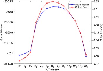
Figure 1 shows social welfare (blue line, left axis) in Equation (1) and the output gap (red line, right axis) as a function of the averaging windows of AIT. Social welfare increases as the window lengthens up to 6 years but begins to decline beyond that point. As is well known, the presence of the ZLB constraint causes welfare losses under IT because the possibility of the ZLB in the future hampers well-anchored inflation expectations. In an economy with AIT, the private sector expects a lower-for-longer policy at the ZLB, resulting in higher inflation and a positive output gap in the future. Since heightened inflation expectations reduce the likelihood of the ZLB binding in the future, welfare losses arising from the ZLB are somewhat alleviated. The window length determines the strength of these effects.
Social welfare/output gap in stochastic steady state.
Note: The blue line (left axis) shows the social welfare in AIT with various averaging windows in each SSS. The red line (right axis) shows corresponding output gaps relative to a flexible price economy.

The blue line shows that for up to 6 years, the expectation effects are favorable enough to reduce welfare losses, causing social welfare to increase. However, as the window length exceeds six years, the optimistic expectations become so strong that output and inflation tend to grow beyond the desired targets. The central bank needs to raise the policy rate to bring inflation back to the target. While this policy action drags inflation closer to the target, output falls below the target due to well-anchored inflation expectations, resulting in higher real interest rates. In other words, overly strong stimulative expectation effects from longer averaging windows hamper social welfare in the long run through reduced output. The red line illustrates this dynamic. As inflation is anchored around the target, what ultimately determines social welfare in the SSS is the output gap.
4.2 The importance of solution method
To evaluate the importance of the solution method in capturing the nonlinear relationship between social welfare and the AIT window, we compare the welfare outcomes obtained using the global method with those derived from a linear approximation. For the latter, given the occasional binding of the ZLB constraint, we employ the method developed by Guerrieri and Iacoviello (Reference Guerrieri and Iacoviello2015), which utilizes a first-order perturbation approach implemented in a piecewise linear framework.
One issue with this method is that the certainty equivalence property holds by the nature of first-order approximation, meaning that agents base their decisions on the expected values of future variables while ignoring higher-order moments such as variance or skewness. As a result, the model’s SSS coincides with its DSS, eliminating the influence of uncertainty on equilibrium dynamics. Consequently, the social welfare in the SSS across different AIT windows is identical.
To address this limitation, we perform a long-run simulation of the model using the linear solution method. Specifically, the model is simulated over 100,000 periods with a series of random shocks, and the first 10,000 periods are discarded as a burn-in to eliminate the influence of initial conditions. The average of the simulated social welfare over the remaining periods is then calculated to approximate the SSS. This approach enables the estimation of the SSS without relying on the flawed certainty equivalence assumption, thereby capturing the effects of future uncertainty on the model’s dynamics more accurately.
For comparison, we apply the same procedure to the model solved using the nonlinear solution method. While this approach does not yield exact welfare values from the fully nonlinear solution, it provides a close approximation of the SSS. Consequently, comparing the SSS derived from the linear solution with the SSS from the nonlinear solution based on these simulations is a reasonable and consistent approach.
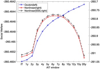
Figure 2 displays the results of the simulations. The red line represents the social welfare from the nonlinear solution method, while the blue line shows the social welfare from the linear solution method. The black dashed line represents the social welfare in the actual SSS shown in Figure 1. The red line and the black dashed line are very close to each other, which implies that social welfare based on simulations is a reasonable proxy for the values in the SSS.
Linear vs nonlinear solution method.
Note: While the blue line (Occbin) represents the results from the method of a first-order perturbation approach, the red line (Nonlinear) represents the results from the global method. The social welfare is calculated based on simulations. The black dashed line (Nonlinear, SSS) shows the SSS social welfare.

The blue line demonstrates that when we solve the model linearly, social welfare increases as the AIT window gets longer. However, if the model is solved nonlinearly, social welfare decreases once the window exceeds 6 years. This occurs because a first-order approximation fails to capture the mechanism through which agents respond to uncertainty in the model. Consequently, the linear solution does not account for the varying probabilities of binding constraints in the future, depending on the window length. This highlights the importance of solving the model nonlinearly when comparing AITs with different windows.
4.3 AIT vs. PLT
Next, we compare AIT with PLT in terms of welfare. Since PLT closely approximates the optimal monetary policy, we use it as a benchmark to evaluate how well AIT performs relative to PLT.Footnote 12 One challenge encountered is that solving the model with
 $\alpha = 0$
in this fully nonlinear framework rendered the model unsolvable. To address this issue, we employ a specific price-level targeting rule:
 \begin{align} R_t^n &= (R_{t-1}^n)^{\rho _R} \bigg [R \bigg (P_t \bigg )^{\phi _{\pi }} \bigg (\frac {y_t}{y}\bigg )^{\phi _{y}} \bigg ]^{1-\rho _R} \exp (\sigma ^{m} \epsilon _t^m), \end{align}
where
 $P_t = \Pi _{t} P_{t-1}$
represents the price level in the current period and the price level target is set to 1.Footnote 13
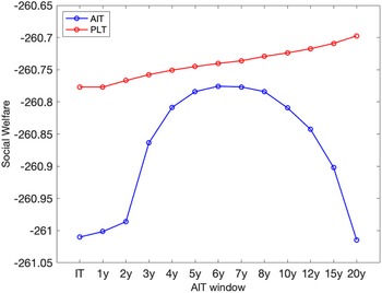
Figure 3 presents the results. Welfare under PLT is consistently higher than under AIT across all window lengths. However, the performance of the 6-year window AIT is notably close to the corresponding PLT outcomes. To provide a clearer interpretation, I translate the welfare losses into consumption-equivalent units.Footnote 14 A 6-year window AIT results in a welfare loss equivalent to a permanent reduction in consumption by 0.02 percent in the PLT economy.
Social welfare of AIT vs. PLT.
Note: The blue line represents social welfare under AIT with various averaging windows in each SSS. The red line represents social welfare under PLT with the same coefficients for inflation responses in the policy rule as in the corresponding AIT framework.

4.4 Macroeconomic biases
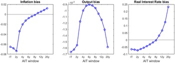
Next, Figure 4 shows how the macroeconomic biases due to the ZLB vary as a function of AIT window length. We examine the biases of inflation, output, and the real interest rate in the SSS, which are computed by taking the difference between their values in the SSS and their corresponding values in the DSS. We observe that medium-length averaging window AITs are effective in mitigating all macroeconomic distortions. In particular, the 8-year window AIT almost closes all three gaps.
Macroeconomic biases.
Note: The inflation bias (left plot), the output bias (middle plot), and the real interest rate bias (right plot) are computed by taking the difference between those values at the SSS and their value at DSS. The inflation and the real interest rate biases are expressed in annualized percentage points and the output gap in percentage points.

One noteworthy observation is that inflation bias and output bias move in opposite directions under longer-window AITs. In these regimes, the downside risk due to ZLB binding is low. However, when the ZLB binds, the private sector anticipates long periods of future inflation and output deviations in the positive direction. This expectation effect is so strong that it outweighs the downside risks. The point at which these two opposing effects balance occurs when the central bank raises the policy rate to mitigate the expectation effects, resulting in high real interest rates and a low output gap.
4.5 Determinants of the optimal 6-year averaging window
An important question in the design of AIT is: What determines the welfare-maximizing averaging period? Addressing this question is essential for understanding how AIT can be effectively implemented in practice. Given the baseline calibration, our numerical results suggest that the optimal averaging period is closely linked to the likelihood of the ZLB being binding.
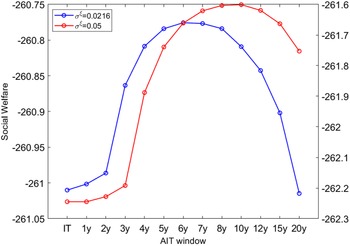
Figure 5 compares the baseline result (blue line) with an alternative scenario (red line) where the standard deviation of preference shocks (
 $\sigma ^{\xi }=0.05$
) is more than doubled. As the standard deviation increases, the economy encounters the ZLB more frequently. Specifically, under the baseline parameterization, the economy is constrained by the ZLB in 10.7% of the state space, whereas in the alternative case, this increases to 11.4%. The figure illustrates that when the probability of the ZLB binding rises, the optimal averaging window lengthens to 10 years.
Social welfare with different level of
 $\sigma ^{\xi }$
.
Note: The blue line (left axis) shows the social welfare in AIT with various averaging windows in each SSS with
 $\sigma ^{\chi }$
= 0.0216. The red line (right axis) shows the social welfare in AIT with various averaging windows in each SSS with
 $\sigma ^{\chi }$
= 0.05. to a flexible price economy.

This finding underscores the critical role of the ZLB in determining the welfare-maximizing length of the AIT window. In scenarios where the ZLB represents a significant constraint, longer averaging windows are advantageous because they more effectively anchor inflation expectations and stabilize the economy. By doing so, they mitigate the adverse effects of constrained monetary policy at the ZLB. Conversely, in environments with a lower likelihood of the ZLB binding, shorter averaging windows are sufficient to achieve similar stabilization benefits without the risk of excessive inflation expectations or overly contractionary future monetary policy.
These results highlight the necessity for policymakers to account for the ZLB probability within their specific economic context when calibrating the averaging window for AIT. A one-size-fits-all approach may fail to address the nuanced trade-offs inherent in different economic environments. This discussion underscores the importance of tailoring AIT design to reflect the unique economic conditions faced by each central bank.
5. Macroeconomic dynamics under AIT
In this section, we study the macroeconomic dynamic properties under various window lengths of AITs. Comparing AITs with different averaging windows is challenging because the information in the past average inflation rates,
 $\hat {\Pi }_{t-1}$
, is not consistent across different regimes. For instance, when the average inflation target is 2%, 1.2% of past average inflation under 4-year window AIT means much larger or longer past inflation losses relative to the value of 1.2% under 2-year window AIT.
To address this issue, we assume that the economies under the different windows of AIT initially remain at their respective SSS whenever we compare dynamics. This ensures that any initial differences among the various regimes do not arise due to differing information in
 $\hat {\Pi }_{t-1}$
. Following this setup, we investigate the primary source of social welfare improvement when AIT is adopted. Specifically, we compare the contributions of two factors: the response to the average inflation rate instead of the period inflation rate, and the higher coefficient of the inflation gap in the policy rule.
Given the same size of shocks across all regimes, the economy under a longer-window AIT stabilizes the dynamics from the shocks more effectively. Based on this, one might expect the marginal welfare gains to be higher in a longer-window AIT economy. According to our simulations, however, this is not the case.
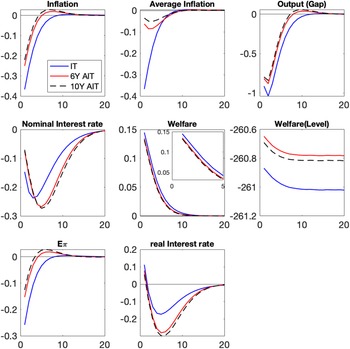
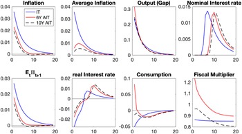
Figure 6 displays the generalized impulse response functions (GIRF)Footnote 15 to negative one-standard-deviation preference shocks under three different monetary policy rules: IT (blue line), 6-year AIT (red line), and 10-year AIT (black dashed line). As the negative shocks hit the economy, inflation falls, but it declines less under AITs. This is due to the well-known expectation channel. Since AITs promise future inflation and a positive output gap to mitigate today’s recession, inflation expectations rise. This can be observed in the left panel of the bottom row. While inflation expectations fall by 0.24% p under IT on impact, they drop by only 0.14% p and 0.11% p under 6-year and 10-year AITs, respectively. Unlike IT, we observe a temporary overshoot of inflation expectations under AIT.
GIRF to preference shocks.
Note: This figure shows GIRF to negative one standard preference shocks in 3 economies with different monetary policy rules. X-axis means horizon. Output is expressed in terms of percentage points, and welfare is the difference between the two figures. The remaining variables are expressed in terms of annualized percentage points.

The small drop in inflation and the longer windows for calculating average inflation result in smaller changes in the average inflation rate under AITs as well. This leads to a larger decrease in the nominal interest rate under IT on impact compared to AIT regimes. However, central banks implementing AITs lower nominal interest rates further to generate inflation expectations afterward. The left panel in the second row demonstrates this dynamic. Due to the low real interest rate under AITs resulting from high inflation expectations, output also falls less on impact and beyond under AITs.
The above dynamics are well-known features of AIT. Here, we additionally report on the dynamics of social welfare. The middle panel in the second row shows the welfare dynamics. It is important to note that this panel does not compare the level of social welfare across the three economies. Instead, it captures marginal changes in social welfare in response to the shocks. The panel illustrates that the marginal gains from each monetary policy are comparable. This finding suggests that the window length of AIT has little effect on the marginal changes in social welfare. This result is somewhat surprising given that a 10-year AIT stabilizes the economy more effectively in terms of average inflation and the output (gap).
The right panel in the second row shows the level of social welfare after the shocks hit the economy. Since each economy begins from its own SSS, a 6-year AIT economy starts at the highest level, followed by a 10-year AIT and IT. Due to the similar marginal effects across regimes, the order of social welfare does not change over the horizon. That is, the level effects dominate the marginal effects.
In the model, adopting AIT introduces two changes to the monetary policy rule. The central bank responds to the average inflation gap instead of the period inflation gap. Additionally, it can respond to the gap more aggressively than under IT. In this subsection, we investigate the effects arising from each component. We refer to the effects due to the former as the targeting effect and those due to the latter as the coefficient effect.
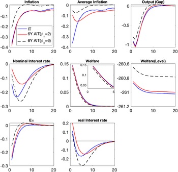
Figure 7 displays the results. The blue line corresponds to the case of IT, which serves as the benchmark. The red line represents a 6-year window AIT with
 $\phi _{\pi }=2$
, and the black dashed line represents a 6-year window AIT with
 $\phi _{\pi }=6$
. Therefore, the gap between the blue line and the red line is interpreted as the targeting effect, while the difference between the red line and the black dashed line is understood as the coefficient effect.
GIRF to preference shocks with different
 $\phi _{\pi }$
.
Note: This figure shows GIRF to negative one standard preference shocks in 3 economies with different monetary policy rules. X-axis means horizon. Output is expressed in percentage points, and welfare is the difference between the two figures. The remaining variables are expressed in terms of annualized percentage points.

Let us first examine the targeting effect. The targeting effect is reflected in the dynamics of nominal interest rates. Due to different targeting objectives, the nominal rates in the red line decline less compared to the IT case. Notably, with the same
 $\phi _{\pi }$
, AIT does not exhibit a lower-for-longer policy, leading to only a modest improvement in inflation expectations. The real interest rates increase further under AIT compared to IT due to the smaller decline in nominal interest rates. Consequently, output falls slightly more than in the blue line case in the short run.
When the central bank responds more aggressively to the average inflation gap, the lower-for-longer policy is implemented, and inflation expectations rise significantly compared to the red line. Both of these factors result in lower real interest rates, leading to a smaller decrease in output. This experiment indicates that it is not the targeting effect but rather the coefficient effect that boosts inflation expectations. Therefore, when the monetary authority transitions from IT to AIT, it is crucial to carefully determine not only the averaging window length but also the aggressiveness of the response to the average inflation gap.
6. The size of the fiscal multiplier
In this section, we study the effects of AIT on the government spending multiplier. As the adoption of AIT changes the behavior of nominal interest rates, inflation expectations, and output, it also affects the multiplier both at the ZLB and outside the ZLB. To analyze this effect, we introduce government spending shocks that follow AR(1) processes instead of monetary policy shocks:
 \begin{align} \ln \frac {g_t}{g} = \rho _{g}\ln \frac {g_{t-1}}{g}+\sigma ^{g}\epsilon _t^{g} \end{align}
where
 $g$
is the steady-state government spending and
 $\epsilon _t^{g} \sim N(0,1)$
. For the baseline parameterization, we set
 $\rho _{g}= 0.81$
and
 $100\sigma ^{g}=0.96$
. To facilitate straightforward computation and enable easy comparison to the literature, we assume no habit in the utility function and no inertia in the monetary policy rule. Following Eggertsson and Singh (Reference Eggertsson and Singh2019), we further assume that the price adjustment costs are not physical menu costs but are perceived only by firms when they maximize their profit.Footnote 16 Therefore, the price adjustment costs do not appear in the resource constraint.
Throughout this section, we report the cumulative fiscal multiplier for output, computed as:
 \begin{align} M(k)=\frac {\Sigma _{s=1}^{k}\frac {\Delta y_{t+s-1}}{\Pi _{j=1}^{s}r_{t+j-1}}}{\Sigma _{s=1}^{k}\frac {\Delta g_{t+s-1}}{\Pi _{j=1}^{s}r_{t+j-1}}} \end{align}
where
 $\Delta$
denotes the level changes between simulated paths with and without a government spending increase, and
 $r_t=E_t\big [\frac {R_t}{\Pi _{t+1}}\big ]$
is the real interest rate.
Since the model is solved nonlinearly, the multiplier depends on the initial state of the economy. We first quantify the multiplier outside the ZLB and then turn to the ZLB case.
6.1 Multiplier outside the ZLB
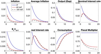
In this subsection, we report the multiplier outside the ZLB. To examine how different window lengths affect the fiscal multiplier, we compare 6-year and 10-year window AITs to IT. Each economy with a different monetary policy rule begins at its own SSS, and government spending increases by 1% following the process described in (12). The results are plotted in Figure 8. The far-right panel in the second row shows the fiscal multipliers. We highlight two key points.
GIRF to government spending shocks and fiscal multiplier outside the ZLB.
Note: Except for output, consumption and fiscal multiplier, the y-axis is the annualized percentage point difference between a path with and without government spending shocks. Output is the difference between two paths scaled by the SSS values. Fiscal multiplier is the cumulative multiplier computed by equation (13).

First, the multipliers under AIT are smaller than in the IT case. Increased demand due to higher government spending leads to a rise in inflation and output. Because of the well-known crowding-out effects, the multiplier remains below unity under IT. In the case of AIT, private agents anticipate a higher-for-longer policy stance from the central bank in response to the inflation gains from increased government spending. This expectation lowers inflation expectations and, consequently, inflation compared to IT. As a result, the nominal interest rate increases less on impact in response to the smaller rise in average inflation rates, but a higher-for-longer policy is implemented thereafter.
The real interest rate mimics the movement of the nominal interest rates. Even though the real rate under AIT is lower than IT on impact, it increases more after a few periods. This is why output under AIT increases less than in the IT case throughout the horizon. The smaller change in output, combined with a larger increase in real interest rates, results in a multiplier lower than in the IT case. In other words, the crowding-out effects become more pronounced under AIT. This is illustrated in the third panel of the second row, which displays the consumption responses.
Second, the multiplier declines as the window length increases. Since the expectation effects under longer-window AIT are stronger, the real interest rates rise more compared to shorter-window AIT. This leads to a greater decline in consumption, resulting in a smaller multiplier in the 10-year AIT case.
One notable point is that the fiscal multiplier outside the ZLB appears higher than reported in the literature. For example, Fernández-Villaverde et al. (Reference Fernández-Villaverde, Gordon, Guerrón-Quintana and Rubio-Ramirez2015) reported a fiscal multiplier of 0.54 on impact outside the ZLB when the model is solved nonlinearly. This discrepancy arises from the fact that the monetary policy rule in our model does not respond to the output gap. If we allowed the central bank to aim at stabilizing the output gap as well, the multiplier would be much lower.Footnote 17 Nevertheless, the points explained above remain robust to this adjustment.
6.2 Multiplier at the ZLB
Next, we investigate the government spending multiplier at the ZLB. Each economy begins at its own SSS in period 0. We inject a series of negative preference shocks in periods 1 and 2 into each economy, which sends the economy under IT to the ZLB, on average, for 5 consecutive quarters. Given the same series of shocks, the economies under AITs experience longer ZLB episodes due to their lower-for-longer policy feature. Government spending rises by approximately 1% in period 2, when the shock ends but the economy still remains at the ZLB. Figure 9 shows the results, and a couple of points are worth highlighting.
GIRF to government spending shocks and fiscal multiplier at the ZLB.
Note: Except for output, consumption and fiscal multiplier, the y-axis is the annualized percentage point difference between a path with and without government spending shocks. Output is the difference between two paths scaled by the SSS values. Fiscal multiplier is the cumulative multiplier computed by equation (13).

First, the multipliers under IT seldom change compared to the outside ZLB case. One reason for this is the flat Phillips curve. The primary channel for government spending to stimulate the economy at the ZLB is through the rise in expected inflation. However, the flat Phillips curve attenuates this channel, limiting the decrease in the real interest rate.Footnote 18 In this sense, the flat Phillips curve weakens the substitution effects of increased government spending.Footnote 19
Another reason is the dominance of the wealth effect over the substitution effect, as evidenced by the decrease in consumption at impact, despite a decline in real interest rates. Since government spending continues to rise even after the economy exits the ZLB due to its persistence, the negative wealth effect dominates the attenuated substitution effect arising from lower real interest rates.
An additional factor is the Rotemberg price adjustment costs. As highlighted by Boneva et al. (Reference Boneva, Braun and Waki2016), these adjustment costs increase firms’ marginal costs in response to government spending shocks, thereby limiting the extent of output expansion.
Second, unlike the IT case, the multipliers under AITs increase for both window lengths. Numerically, the multipliers at impact are approximately 1.23 and 0.96 for 6-year and 10-year AIT, respectively, compared to values below 0.8 outside the ZLB for both. Under AIT, agents anticipate longer ZLB episodes, leading to a greater rise in inflation expectations. This partially restores the weakened substitution effect.
The restored substitution effect under 6-year AIT is strong enough to dominate the wealth effect, resulting in increased consumption and a fiscal multiplier above one at impact. Conversely, under a 10-year AIT, inflation expectations rise less than under a 6-year AIT, meaning the restored substitution effect cannot overturn the dominance of the wealth effect. As a result, the multiplier at impact does not exceed one, although it remains significantly higher than outside the ZLB.
To summarize, as the recession becomes more severe, fiscal policy under AIT proves more effective compared to IT. This result assumes a very flat Phillips curve and persistent government spending, which is broadly supported by empirical evidence
7. Sensitivity analysis
In this section, we conduct several sensitivity analyses for social welfare in the SSS and the fiscal multiplier, respectively.
7.1 Social welfare in SSS
In Section 4, we show that social welfare increases non-monotonically with the AIT window length. In this subsection, we examine how robust this result is under different assumptions: no habit, the same value of
 $\phi _{\pi }(=2)$
, the response of the monetary policy rule to the output gap, and a steep Phillips curve.
Figure 10 shows the results. The first left panel in the first row corresponds to the case of no habit. The presence of habit does not affect the nonlinear property of social welfare, though it significantly changes the level of social welfare across all window lengths. One might speculate that the nonlinear property arises from the different responses to the inflation gap in the monetary policy rule. However, this turns out not to be the case.
Social welfare in SSS in various environments.
Note: No habit means
 $h=0$
in the model.
 $\phi _{\pi }=2$
is the case when the response to the inflation gap in the monetary policy rule remains unchanged across AIT windows.
 $\phi _{y}=0.1$
is the case when the central bank responds to the output gap in addition to the inflation gap with baseline parameterization of
 $\phi _{\pi }$
. Steep NKPC corresponds to the case of smaller
 $\varphi$
.

The right panel of the first row shows the results when the response to the inflation gap in the monetary policy rule remains fixed at
 $\phi _{\pi }=2$
across all AIT windows. While the welfare gains from short to medium windows are minimal, the welfare losses from medium to long windows appear substantial. This occurs because, with a fixed low value of
 $\phi _{\pi }$
, the stability of inflation and the output gap deteriorates as the averaging window lengthens. This observation raises the possibility that, with a fixed but higher value of
 $\phi _{\pi }$
, the welfare under IT could exceed the welfare achieved under AIT for any window length. We confirm this conjecture, and the results are presented in Appendix E.Footnote 20
Next, we investigate the case of
 $\phi _{y}=0.1$
, a form of extended AIT, and the steep Phillips curve. The second row of the figure corresponds to these scenarios. Neither of them alters the nonlinear properties. The lack of significant differences between the extended AIT and the baseline AIT could stem from the growing importance of addressing inflation gaps in both frameworks and the anchoring of expectations under credible policy.
7.2 Fiscal multiplier
In Section 6, we show how the fiscal multiplier changes with the AIT window length both outside the ZLB and at the ZLB. In this subsection, we examine how robust these results are under different assumptions: a steep NKPC, the response of the monetary policy rule to the output gap, and less persistent government spending shocks. Figure 11 displays the results. The first column shows the multipliers outside the ZLB, while the second column corresponds to the ZLB case.Footnote 21
Fiscal multipliers in various environments.
Note: Fiscal multiplier is the cumulative multiplier computed by equation (13). The first row shows the multipliers when the slope of the linearized Phillips curve is 0.03 instead of the baseline case of 0.01. The second row corresponds to the monetary policy rule responding to the output gap as well as the inflation gap. While the third row displays the case of less persistent government spending shocks, the last row shows the case of
 $\phi _{\pi }=2$
for AITs. The blue line, red line and black line represent IT, 6-year AIT, and 10-year AIT, respectively. The y-axis represents the size of the fiscal multiplier for all panels.

Steep Phillips curve The first row shows the multipliers when the slope of the linearized Phillips curve is 0.03, compared to the baseline value of 0.01. As mentioned earlier, the flat Phillips curve attenuates substitution effects. In contrast, with a steep NKPC, substitution effects are restored, causing the fiscal multiplier of IT at the ZLB to rise above two on impact, which is larger than the multipliers for 6-year or 10-year AIT.
Outside the ZLB, the multipliers are lower than in the baseline case. This is because inflation rises more sharply with the steep NKPC in response to the increase in government spending. The central bank reacts by raising nominal interest rates more than the increase in inflation, which drives real interest rates higher. As a result, the output increase is smaller compared to the baseline case for all three policy rules.
Response to output gap in the monetary policy rule The second row corresponds to the inclusion of a response to the output gap in the monetary policy rule. We assume
 $\phi _{y}=0.1$
, a value widely used in the literature.Footnote 22 Outside the ZLB, the multipliers are again lower than in the baseline case because the central bank raises nominal interest rates more aggressively, responding to both inflation and output gains. This reinforces crowding-out effects, causing the multipliers to decline.
At the ZLB, the inclusion of
 $\phi _{y}$
lengthens the ZLB episodes. As a result, the increase in government spending raises inflation expectations and lowers real interest rates further relative to the baseline case. This effect is substantial enough for the IT case to overturn the dominance of the wealth effect, causing the at-impact multiplier to exceed two. In contrast, under AIT, inflation expectations show little change compared to the baseline case, even with the inclusion of
 $\phi _{y}$
. This is reflected in the similar dynamics of multipliers in both cases. The reason is that the response to the output gap does not significantly lengthen the expected ZLB duration under AIT, where the duration is already extended by the adoption of AIT itself.
Less persistent government spending shocks The third row displays the multiplier with less persistent government spending processes, where we assume
 $\rho _{G}=0.5$
instead of 0.81. Less persistent processes imply a smaller wealth effect, regardless of whether the ZLB is binding. As shown in the left panel, the multipliers outside the ZLB are significantly higher and approach unity for the IT case due to the reduced wealth effect. While the multipliers under AIT also increase, they remain lower than those under IT.
At the ZLB, the multiplier also increases relative to the baseline case. Nevertheless, the multipliers are not significantly different from the baseline case, indicating that the attenuated substitution effect caused by the flat Phillips curve remains strong.
Smaller response to the inflation gap in the monetary policy rule The last row shows the case where
 $\phi _{\pi }=2$
for AITs in the monetary policy rule. The smaller response to the inflation gap arising from the increase in government spending results in a smaller rise in the policy rate and a greater increase in inflation expectations. This leads to a much lower real interest rate, mitigating the crowding-out effects. Consequently, unlike the baseline case, the fiscal multipliers under AIT at impact are higher than those under IT.
At the ZLB, the multipliers are not significantly different from those outside the ZLB, as shown in the baseline IT case. The smaller response to the inflation gap reduces the lower-for-longer policy effect, resulting in similar ZLB durations under IT and AIT. Therefore, the real interest rates fall less than in the baseline case, weakening the substitution effects. Given the flat Phillips curve and persistent government spending, the wealth effect dominates, and consumption under AIT decreases similarly to the IT case.
8. Conclusion
In this paper, we demonstrate that the length of the averaging window in AIT significantly influences equilibrium dynamics, as agents form their expectations differently depending on the window length. Social welfare increases with medium-length windows but declines once the window surpasses a certain threshold. This non-monotonic result emerges only when the model is solved nonlinearly, highlighting the importance of using global methods to comprehensively analyze AIT.
We also investigate the impact of AIT on the fiscal multiplier both outside and at the ZLB. Outside the ZLB, the fiscal multiplier under AIT is lower than under IT due to reduced inflation expectations and a higher-for-longer policy stance, which amplifies the crowding-out effect. These effects become more pronounced as the averaging window lengthens. At the ZLB, however, AIT enhances the effectiveness of government spending compared to IT. With a flat Phillips curve and persistent government spending processes, the fiscal multiplier under IT remains relatively unchanged from its value outside the ZLB. In contrast, under AIT, the lower-for-longer policy reinforces inflation expectations, resulting in fiscal multipliers exceeding one for certain window lengths.
Our study primarily focuses on how welfare evolves as the averaging window lengthens. However, we encountered a limitation: the model becomes unsolvable for windows longer than 20 years using current nonlinear solution methods. This technical constraint prevents us from fully analyzing the transition from medium- to long-term windows and understanding how AIT converges to PLT in terms of welfare. Consequently, our conclusions are based on comparisons between short- to medium-term windows, finding that a 6-year window achieves the highest welfare within the feasible range. While we observe an upward trend in welfare as the window length increases in this range, we cannot definitively determine whether this trend continues and fully converges to PLT. This acknowledged limitation underscores the need for further research to refine solution methods and analyze longer windows.
Despite these limitations, our analysis provides important insights into the practical implementation of AIT. Central banks are more likely to adopt AIT policies with finite averaging windows rather than infinite ones. Understanding how AIT performs within a realistic range of window lengths is, therefore, critical, and our finding that a 6-year window optimally balances welfare represents a valuable contribution.
Moreover, our results highlight the trade-offs inherent in selecting an averaging window length: welfare initially improves but diminishes with overly long windows due to agents’ expectations of excessive policy accommodation, particularly when the probability of ZLB binding is high. The likelihood of ZLB binding plays a key role in determining the optimal window length, as longer windows are more effective in stabilizing inflation expectations in economies frequently constrained by the ZLB. Conversely, in environments with a lower likelihood of ZLB episodes, shorter windows may suffice to achieve stabilization without the risks associated with excessive accommodation.
These findings emphasize that the optimal averaging window length should reflect the economic context, especially the probability of ZLB episodes. Policymakers must carefully balance short-term flexibility with long-term price stability, ensuring that AIT frameworks are tailored to the specific structural characteristics of their economies. By recognizing the influence of ZLB binding probabilities, this study provides a nuanced understanding of the trade-offs involved in designing AIT policies. In this sense, our analysis offers robust and actionable insights for shaping effective monetary policy within a feasible and practical framework.
Acknowledgements
I would like to particularly express my thanks to the anonymous two referees and the editor.
Supplementary material
The supplementary material for this article can be found at https://doi.org/10.1017/S1365100525100527.