1. Introduction
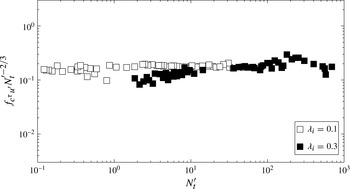
Magnetohydrodynamic (MHD) turbulence at low magnetic Reynolds number has a well-known tendency to become two-dimensional. In this paper, we experimentally characterise the mechanisms through which two-dimensionality breaks down in these flows and quantify the ensuing three-dimensionality. Besides the fundamental question of understanding this type of turbulence, liquid metal flows, in which MHD turbulence is usually found, are of central industrial interest. In the metallurgical and nuclear sectors, they are either processed or used to carry heat and mass. Typical examples include fourth-generation sodium nuclear fission reactors and the cooling blankets of nuclear fusion reactors (Vetcha et al.
Reference Vetcha, Smolentsev, Abdou and Moreau2013). Since two- and three-dimensional turbulence have radically different transport and dissipation properties, the question of the dimensionality of turbulence is key to the efficiency of these systems. In such engineering configurations, the flow is neither intense nor electrically conductive enough to advect the magnetic field over a short enough time to compete with magnetic diffusion. This justifies their description in the frame of the low-
 $\mathit{Rm}$
approximation, where the coupling between electrical and mechanical quantities reduces to that between velocity, pressure and local electric current density (Roberts Reference Roberts1967). Under this approximation, Sommeria & Moreau (Reference Sommeria and Moreau1982) showed in a seminal paper, to which the title of this work pays homage, that the main effect of the Lorentz force was to diffuse the momentum of a structure of size
 $l_{\bot }$
along the externally applied magnetic field
 $\boldsymbol{B}$
in time
 ${\it\tau}_{2D}=({\it\rho}/{\it\sigma}B^{2})(l_{z}/l_{\bot })^{2}$
over a distance
 $l_{z}$
(
 ${\it\rho}$
and
 ${\it\sigma}$
are the fluid density and electric conductivity). This effect explains the tendency of these flows to two-dimensionality when the field is homogeneous. When turbulence is present, diffusion is achieved over a distance
 $l_{z}^{(N)}\sim N^{1/2}$
, where the interaction parameter
 $N$
is the ratio of the eddy turnover time
 ${\it\tau}_{U}(l_{\bot })=l_{\bot }/U(l_{\bot })$
to the Joule dissipation time
 ${\it\tau}_{J}={\it\rho}/{\it\sigma}B^{2}$
. This remarkable property was exploited extensively to reproduce some of the fine properties of two-dimensional turbulence, such as the inverse energy cascade, in thin horizontal layers of liquid metal pervaded by a strong vertical magnetic field (Sommeria (Reference Sommeria1986, Reference Sommeria1988); see figure 3 for a generic representation of this geometry). It also places MHD flows in the much wider class of flows with a tendency to two-dimensionality: this class includes flows in a background rotation Greenspan (Reference Greenspan1969) or where stratification is present Paret et al. (Reference Paret, Marteau, Paireau and Tabeling1997). Geophysical flows (oceans and atmospheres) are famous examples. The question of the dimensionality of turbulence in plane fluid layers is key to understanding the dynamics of all such systems.
In low-
 $\mathit{Rm}$
MHD, the question of dimensionality emerged with numerical simulations in bounded domains: Schumann (Reference Schumann1976) showed the first evidence of MHD turbulence becoming strictly two-dimensional in a three-dimensional periodic domain when
 $N$
was significantly greater than unity, and this was later confirmed by Zikanov & Thess (Reference Zikanov and Thess1998). More recently, Boeck, Krasnov & Thess (Reference Boeck, Krasnov and Thess2008) found, still numerically, that at moderate values of
 $N$
, the flow could shift intermittently between two- and three-dimensional states. Thess & Zikanov (Reference Thess and Zikanov2007) found the same phenomenon in ellipsoidal structures confined by slip-free boundaries, while Pothérat & Dymkou (Reference Pothérat and Dymkou2010) showed that for a flow in a given magnetic field, three-dimensionality appeared at a bifurcation when the intensity of a two-dimensional flow with a velocity field orthogonal to the magnetic field (2D-2C flow), was increased. All of these studies with dissipation-free boundaries drew a picture where three-dimensionality developed as an instability on initially two-dimensional (and two-component) flows.
By contrast, strict two-dimensionality cannot be achieved when physical walls are present, as in experiments or in oceans and planetary atmospheres, because of the three-dimensionality of wall boundary layers. Furthermore, friction there drives mass or electric current (respectively in rotating and MHD flows), that recirculate in the core under the form of Ekman pumping or eddy currents. Owing to this effect, transversal components of velocity or electric current almost always subsist in thin layers of fluid, even when weak boundary friction is present. This was observed both in non-MHD (Akkermans et al.
Reference Akkermans, Kamp, Clercx and Van Heijst2008) and MHD flows. Not only does it affect the quasi-two-dimensional dynamics of the flow but it also induces three-dimensionality in the core (Alboussière, Uspenski & Moreau Reference Alboussière, Uspenski and Moreau1999; Pothérat, Sommeria & Moreau Reference Pothérat, Sommeria and Moreau2000, Reference Pothérat, Sommeria and Moreau2005). Asymptotic analyses indeed predict a quadratic variation of velocity across the bulk of the fluid layer, called the barrel effect (Pothérat et al.
Reference Pothérat, Sommeria and Moreau2000; Pothérat Reference Pothérat2012), which was observed in the numerical simulations of (Mück, Günter & Bühler Reference Mück, Günter and Bühler2000). An inhomogeneous forcing across the fluid layer was shown to drive three-dimensionality too, and the resulting three-dimensional structures were recently found to induce secondary flows that could override Ekman pumping (Pothérat et al.
Reference Pothérat, Rubiconi, Charles and Dousset2013). These results concur to show that whether induced by the boundaries or by the inhomogeneity of the forcing, (i) the appearance of three-dimensionality and the appearance of the third velocity component are interdependent, and (ii) three-dimensionality does not always result from instabilities, at least in wall-bounded flows. Our previous experiments in fact suggest that three-dimensionality due to recirculating flows or electric currents and instability-driven three-dimensionality could co-exist, but tended to take distinct forms: respectively a weak form, where only the flow intensity varies along
 $\boldsymbol{B}$
, and a strong form, where flow topology varies too (Klein & Pothérat Reference Klein and Pothérat2010). Recently, it was also shown that because three-dimensional flows are more dissipative, they carry less energy than their quasi-two-dimensional counterpart for the same level of external forcing and they also decay faster when not forced. This property was used to detect three-dimensionality in non-MHD flows (Duran-Matute, Trieling & van Heijst Reference Duran-Matute, Trieling and van Heijst2010; Shats, Byrne & Xia Reference Shats, Byrne and Xia2010).
Our purpose is to characterise three-dimensionality in low-
 $\mathit{Rm}$
MHD turbulence in wall-bounded fluid layers and to determine its driving mechanism. Our starting point shall be to quantify how flow intensity varies with dimensionality, somewhat in the spirit of Duran-Matute et al. (Reference Duran-Matute, Trieling and van Heijst2010). Our approach consists of forcing turbulence between two walls orthogonal to an externally imposed magnetic field in a thick enough layer of fluid to observe how three-dimensionality develops. We shall first describe how the experimental set-up can reproduce the generic properties of MHD turbulence in channels (§ 2). We shall then establish theoretical scalings linking near-wall velocities to the intensity of the electric current driving flows in MHD channels (§ 3). Occurrences of three-dimensionality will then be tracked in the light of these scalings (§ 4) and an experimental measure of the corresponding values of
 $l_{z}^{(N)}$
shall be obtained (§ 5). This picture shall finally be refined by means of frequency analysis and through a quantitative measure of weak and strong three-dimensionalities (§ 6).
2. The FLOWCUBE experimental facility
2.1. Mechanical description
The principle of the experiment follows that of Sommeria (Reference Sommeria1986) on quasi-two-dimensional turbulence in which a constant, almost homogeneous magnetic field
 $\boldsymbol{B}=B\boldsymbol{e}_{z}$
was applied across a square, shallow container of height
 $0.02\ \text{m}$
filled with liquid mercury (the frame origin is chosen at the centre of the bottom wall, with
 $\boldsymbol{e}_{x}$
and
 $\boldsymbol{e}_{y}$
pointing along its edges). References to top and bottom walls are used for convenience, since gravity plays no relevant role in this experiment. In this configuration, the time scale for two-dimensionalisation
 ${\it\tau}_{2D}(l_{\bot })$
for each flow structure of transverse size
 $l_{\bot }$
was less than
 $10^{-2}\ \text{s}$
and much smaller than its turnover time
 ${\it\tau}_{U}(l_{\bot })$
. The flow was assumed quasi-two-dimensional on these grounds. Unlike this earlier experiment though, the present container is not shallow, but cubic with inner edge
 $h=0.1\ \text{m}$
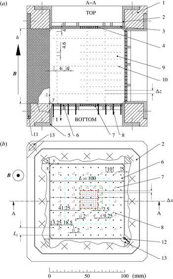
(figure 1). Walls are impermeable and electrically insulating, except where small electrodes are inserted, either to drive or diagnose the flow. Since Hartmann and Shercliff layers are expected to develop along walls perpendicular and parallel to
 $\boldsymbol{B}$
, we shall refer to them as Hartmann walls and Shercliff walls, respectively (figures 1 and 2). For the lower magnetic fields used,
 ${\it\tau}_{2D}(l_{\bot })$
is of the order of
 $1\ \text{s}$
. Such times are much longer than those of Sommeria (Reference Sommeria1986), and potentially comparable to, or longer than eddy turnover times, so three-dimensionality is expected to be present. The working liquid metal is Gallinstan (or MCP11), an eutectic alloy of gallium, indium and tin that is liquid at room temperature, with electric conductivity
 ${\it\sigma}=3.4\times 10^{6}\ \text{S}\ \text{m}^{-1}$
, density
 ${\it\rho}=6400\ \text{kg}\ \text{m}^{-3}$
and viscosity
 ${\it\nu}=4\times 10^{-7}\ \text{m}^{2}\ \text{s}^{-1}$
. The container is successively filled with argon and evacuated several times so as to ensure that as little gas as possible remains inside the vessel, and to prevent oxidation of the Gallinstan as much as possible. This way, the liquid metal is in the tightest mechanical contact with the walls and in electrical contact with all wall-embedded electrodes. Once filled with Gallinstan, the container is subjected to a magnetic field
 $B\boldsymbol{e}_{z}$
by being placed at the centre of the cylindrical bore of a superconducting solenoidal magnet. Magnetic fields
 $B\in [0.1,5]\ \text{T}$
of a maximum inhomogeneity of
 $3\,\%$
along
 $\boldsymbol{e}_{x}$
,
 $\boldsymbol{e}_{y}$
and
 $\boldsymbol{e}_{z}$
and with corresponding Hartmann numbers
 $\mathit{Ha}=\mathit{Bh}({\it\sigma}/({\it\rho}{\it\nu}))^{1/2}\in [364,18\,222]$
are achieved (
 $\mathit{Ha}^{2}$
measures the ratio of Lorentz to viscous forces, see § 3). This very low level of inhomogeneity is not expected to have any significant effect on the measurements. By contrast, a possible curvature of the magnetic field lines due to the bipolar structure of the magnetic field could have an influence on the diagnosis of three-dimensionality. By comparing the position of several vortex centres in a steady quasi-two-dimensional regime using interpolation between probes, we found that the lateral streamline displacement between top and bottom walls was approximately the size of an injection electrode (1 mm), which is below the spatial resolution of our measurements. The lack of influence of inhomogeneity was also confirmed by the very low level of three-dimensionality we measured in the asymptotic quasi-two-dimensional regime (§ 6).
Sketch of the cubic container. (a) Cross-section. (b) Top view onto the bottom plate: (1) cubic brazen frame; (2) top plate with (3) top electronic board (top Hartmann wall); (4) set of 196 potential probes from the top Hartmann wall; (5) bottom plate with (6) bottom electronic board (bottom Hartmann wall); (7) set of 196 potential probes from the bottom Hartmann wall (as on the top plate) and (8) additional 100 forcing electrodes; (9) electronic board at the Shercliff wall with (10) 195 potential probes; (11) side plate; (12) probe for electric potential reference; (13) inlet and outlet to evacuate the container and to fill it with liquid metal. All container walls are electrically insulating, except at the locations of potential probes and current injection electrodes. The central square region with high density of electric potential probes on the Hartmann walls is marked with a (red online) dashed line.

The flow entrainment relies on the same principle as in Sommeria’s (Reference Sommeria1986) and Klein, Pothérat & Alferjonok’s (Reference Klein, Pothérat and Alferjonok2009) experiments. A DC electric current in the range
 $I\in [0{-}300]\ \text{A}$
is injected at the bottom Hartmann wall located at
 $z=0$
(figure 1), through a lattice of either
 $n=100$
or
 $n=16$
electrodes, each of diameter
 $1\ \text{mm}$
. The basic forcing geometry consists of a square array of either
 $10\times 10$
or
 $4\times 4$
electrodes respectively spaced by distances of either
 $L_{i}=0.01\ \text{m}$
or
 $L_{i}=0.03\ \text{m}$
(non-dimensionally,
 ${\it\lambda}_{i}=L_{i}/h=0.1$
or
 ${\it\lambda}_{i}=0.3$
), both centred on the bottom Hartmann plate. For high enough injected current, this basic pattern turns into turbulence, with adjustable forcing scale
 ${\it\lambda}_{i}$
. The electrodes are made of copper and gold plated, which ensures provision of a good electrical contact with the Gallinstan. They are embedded into the bottom Hartmann wall located at
 $z=0$
, and mounted flush so that they do not protrude into the liquid metal and bring no mechanical disturbance into the flow. At their other end, they are connected to a regulated DC power supply through a dedicated switchboard system. This system makes it possible to connect each of the 100 available electrodes to either the positive or the negative pole of the DC power supply or to leave it open-ended. The
 $10\times 10$
and
 $4\times 4$
arrays are obtained by alternately connecting all of the electrodes to either pole (
 $10\times 10$
), or by leaving two unconnected electrodes between one connected to the positive pole and one connected to the negative pole (
 $4\times 4$
). For low injected electric current
 $I$
, the base flow consists of vortices of diameter
 $L_{i}$
spinning in alternate directions as in Sommeria’s (Reference Sommeria1986) experiment. This type of set-up and forcing allowed Sommeria (Reference Sommeria1986) to provide one of the first experimental evidences of the inverse energy cascade, a distinctive feature of two-dimensional turbulence. In that sense, the constant periodic forcing generates quasi-two-dimensional turbulence at high
 $N$
when the injected current sufficiently exceeds the critical value for the destabilisation of the array. It should also be noted that a constant forcing is necessary to study the dimensionality of MHD turbulence as we set out to do. Without it, three-dimensionality would be suppressed by the action of the Lorentz force and turbulence would decay over timescales of the order of
 ${\it\tau}_{2D}(L_{i})$
or of the Hartmann friction time, depending on whether it is three- or quasi-two-dimensional (Sommeria & Moreau Reference Sommeria and Moreau1982).
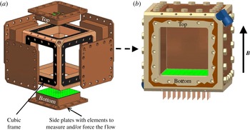
Modular design based on a cubic frame with interchangeable side plates. These plates can be easily swapped to exchange flow forcing and flow measurement systems. (a) Open container with side plates unmounted. (b) Closed container where the front plate is only partly represented to allow for a view into the container.

Since all electrodes are connected to a single power supply, particular attention was paid to ensure that the same, constant current intensity
 $I$
passed through all of them, despite random fluctuations in the contact resistance between the electrode surface and the liquid metal. These fluctuations of amplitude of the order of
 $10^{-2}\ {\rm\Omega}$
can lead to an irregular current distribution resulting into an ill-controlled forcing. By adding a constant ohmic resistance of
 $2\ {\rm\Omega}\pm 0.25\,\%$
to all 100 electric circuits, the impact of these fluctuations on the uniformity of the forcing becomes negligible. Each
 $2\ {\rm\Omega}$
resistance dissipates a maximal power of
 $100\ \text{W}$
, which limits the injected electric current per electrode to approximately
 $7\ \text{A}$
. To evacuate heat, they are mounted on water-cooled aluminium plates. The current injected in each electrode is monitored prior to each acquisition and discrepancies between the values measured at each electrode were found to remain on the order of
 $0.25\,\%$
.
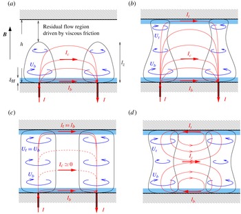
Schematic representation of generic flow configurations in a channel in an external magnetic field. Hartmann layers are represented as semi-transparent strips in light blue, paths of electric current in red (marked
 $I_{b}$
,
 $I_{t}$
and
 $I_{c}$
), and fluid flow as blue, circular arrows. (a)
 $l_{z}\ll h$
, the injected current spreads between the Hartmann layer and the core, where the Lorentz force it generates balances either viscous or inertial forces; (b)
 $l_{z}\gtrsim h$
, same as (a) but part of the injected current flows into the top Hartmann layer, the flow is three-dimensional and influenced by the top wall; (c)
 $l_{z}\gg h$
, the current spreads equally between top and bottom Hartmann layers, with practically no leak into the core; the flow is quasi-two-dimensional; (d) symmetrically three-dimensional structures, not attached to electrodes and where eddy currents in the core are equally sourced from both Hartmann layers.

2.2. Electric potential measurements
The flow is analysed by measuring the electric potential
 ${\it\phi}$
locally, at probes that are embedded in the container walls. Each electric potential is obtained with respect to a reference taken in the thin inlet pipe located in a corner of the vessel, where the liquid metal is always at rest (see figure 1). Each probe consists of a gold-plated copper wire 0.2 mm in diameter fitted flush to the container wall, in the same way as the current injection electrodes are. This way, they incur practically no mechanical nor electrical disturbance on the flow. 196 of these probes are embedded in the
 $x{-}y$
plane, in the bottom
 $(z=0)$
and top
 $(z=h)$
Hartmann walls, and 195 probes in the
 $y{-}z$
plane at the Shercliff wall at
 $x=0$
. The sets of potential probes embedded in the top and bottom Hartmann walls are mirror symmetric and precisely aligned opposite each other along magnetic field lines. Near the centre of the Hartmann walls, probes are positioned in a dense
 $10\times 10$
grid of spacing
 ${\rm\Delta}x={\rm\Delta}y={\rm\Delta}=2.5\ \text{mm}$
to map the smaller spatial variations of potential. We shall refer to this region of the
 $(x,y)$
plane as the ‘central square’ ((red online) dashed line in figure 1). Mid-size and box-size structures are captured by measurements on sets of three probes (distant by
 ${\rm\Delta}x={\rm\Delta}y=2$
mm from one another so as to record local variations of
 ${\it\phi}$
along
 $\boldsymbol{e}_{x}$
and
 $\boldsymbol{e}_{y}$
), around the centre array and further out close to the Shercliff walls (figure 1). On the Shercliff wall at
 $x=0$
, probes are respectively spaced by
 ${\rm\Delta}y=4\ \text{mm}$
and
 ${\rm\Delta}z=4.6\ \text{mm}$
along
 $\boldsymbol{e}_{y}$
and
 $\boldsymbol{e}_{z}$
. Signals recorded there give an insight on the structure of the flow along the magnetic field lines (see § 5).
The signals are collected via a printed circuit leading to 16-pin connectors built-in at the back of all walls. From there, the signal is conveyed to a high-precision single-ended 736-channel acquisition system, manufactured and tailored to this particular experiment by company NEUROCONN (http://www.neuroconn.de/profile/). Since the signals can be of the order of
 $10\ {\rm\mu}\text{V}$
, each channel features a low-noise amplifier with gain 111. All signals are then synchronously sampled to
 $24$
-bit precision at a frequency of
 $128\ \text{Hz}$
. Digital signals are optically transmitted to a PC where they are recorded through a dedicated MATLAB/SIMULINK module. Since frequencies relevant to the flow are typically expected in the range
 $[0,35]\ \text{Hz}$
, each channel is fitted with a low-pass filter of cut-off frequency of
 $45\ \text{Hz}$
. The peak-to-peak background noise that remains on the filtered signal is less than
 $2\ {\rm\mu}\text{V}$
, and this determines the precision of the measurement system. The high dynamic range dedicated analogue-to-digital (A/D) conversion on each channel combined with the absence of detectable drift in the signals guarantees that no loss in precision occurs when subtracting the signals from neighbouring probes to construct gradients of electric potential.
The measurement chain provides real-time simultaneous time series of electric potential in 587 locations spread between the top and bottom Hartmann walls and on one of the Shercliff walls (thereafter denoted
 ${\it\phi}_{b}$
and
 ${\it\phi}_{t}$
and
 ${\it\phi}_{S}$
). At the Hartmann walls, gradients of electric potential at
 $\boldsymbol{r}$
shall be determined from a second order approximation:
 $$\begin{eqnarray}\boldsymbol{{\rm\nabla}}_{\bot }{\it\phi}(\boldsymbol{r})=\frac{1}{{\rm\Delta}}\left[\begin{array}{@{}c@{}}\displaystyle {\it\phi}\left(\boldsymbol{r}+\frac{{\rm\Delta}}{2}\boldsymbol{e}_{x}\right)-{\it\phi}\left(\boldsymbol{r}-\frac{{\rm\Delta}}{2}\boldsymbol{e}_{x}\right)\\ \displaystyle {\it\phi}\left(\boldsymbol{r}+\frac{{\rm\Delta}}{2}\boldsymbol{e}_{y}\right)-{\it\phi}\left(\boldsymbol{r}-\frac{{\rm\Delta}}{2}\boldsymbol{e}_{y}\right)\end{array}\right]+\mathit{O}({\rm\Delta}^{3}).\end{eqnarray}$$
Electric potentials measured on Hartmann walls can also be related to the velocity fields
 $\boldsymbol{u}_{b}$
and
 $\boldsymbol{u}_{t}$
in the bulk of the flow just outside the Hartmann layers using Ohm’s law there, and neglecting variations of potential across the Hartmann layers, which are of the order of
 $\mathit{Ha}^{-2}$
. For the bottom wall,
 $$\begin{eqnarray}\boldsymbol{u}_{b}=B^{-1}\boldsymbol{e}_{z}\times \boldsymbol{{\rm\nabla}}_{\bot }{\it\phi}_{b}+({\it\sigma}B)^{-1}\boldsymbol{e}_{z}\times \boldsymbol{J}_{b},\end{eqnarray}$$
where
 $\boldsymbol{J}_{b}$
is the current density just outside the Hartmann layer. In quasi-two-dimensional flows,
 $\boldsymbol{J}_{b}\sim {\it\sigma}BUHa^{-1}$
can be neglected. Equation (2.2) then provides an indirect measurement of the velocity field, which has been widely used in MHD experiments featuring thin fluid layers (Alboussière et al.
Reference Alboussière, Uspenski and Moreau1999). Kljukin & Thess (Reference Kljukin and Thess1998) further noticed that in this case, the streamfunction in the bulk becomes proportional to
 ${\it\phi}_{b}$
and so isolines of
 ${\it\phi}_{b}$
provide a direct visualisation of flow patterns. When the flow becomes three-dimensional, however,
 $\boldsymbol{J}_{b}$
becomes larger but still depends on the mechanism which pulls current in the core. For instance, we shall see in § 3 that when inertial effects are present,
 $\boldsymbol{J}_{b}=\mathit{O}(N^{-1})$
, so even in this case, flow patterns can still be identified and velocities estimated from (2.2), albeit with a precision that decreases with
 $N^{-1}$
(see Sreenivasan & Alboussière (Reference Sreenivasan and Alboussière2002), where errors incurred by this measurement technique are estimated). We shall follow this strategy to test the scaling laws derived in § 3 against our measurements. We shall also obtain an alternative, more precise quantification of three-dimensionality, using potential measurements directly in § 6. For this, we shall rely on the property that in a quasi-two-dimensional flow, measurements of electric potentials and their gradient taken at the top and bottom Hartmann walls should be fully correlated, whereas any trace of three-dimensionality should translate into a loss of correlation between these quantities.
2.3. Experimental procedure and strategy
Experiments are performed at a constant magnetic field (constant
 $\mathit{Ha}$
). Starting from a flow at rest, the current per electrode, (measured non-dimensionally by parameter
 $\mathit{Re}^{0}$
defined in § 3), is increased in approximately 20 steps, spread logarithmically between 0 and 6 A. At each step, electric potentials were recorded in a statistically steady state, which was deemed reached after typically
 $5{\it\tau}_{H}$
, where the Hartmann friction time
 ${\it\tau}_{H}=h^{2}/(2{\it\nu}Ha)$
, which characterises quasi-dimensional dynamics (Sommeria & Moreau Reference Sommeria and Moreau1982), is much longer than
 ${\it\tau}_{J}$
which characterises three-dimensional effects. Records extended over a maximum of 7–10 min, imposed by limitations of the cooling system for the superconducting magnet. To ensure stability of the magnetic field, the magnet was operated in ‘persistent mode’, i.e. with the coil disconnected from its power supply. Variations of magnetic field remained unmeasurable over a much longer time than the few consecutive hours needed to record data at one given field.
Forcing the flow at one wall only imposes a particular topology to the forcing that allows us to derive crucial generic information on the properties of MHD turbulence in channels. First, the flow is forced near the bottom wall, where current is injected, but free near the top wall. Comparing flows in the vicinity of both walls therefore gives us a reliable way to quantify three-dimensionality. Second, the influence of the top wall depends only on the dimensionality of turbulence and should therefore reflect the generic properties of walls in MHD turbulence in channels (§ 4). Finally, by analysing electric potentials along
 $\boldsymbol{B}$
at the side wall, we shall be able to identify the trace of the forcing and distinguish the properties of turbulence that are linked to it from generic ones: forcing-dependent and forcing-independent properties shall indeed be segregated on the grounds that since current is injected at one wall only, the dimensional trace of the forcing is carried by the antisymmetric part of these profiles, while their symmetric part is relatively independent of the forcing (§ 5). Driving the flow in this manner offers a very general way to parametrise a wide range of forcing types: any force density
 $\boldsymbol{f}$
applied to the flow can indeed be characterised by its intensity and geometry. The former can be measured through the current
 ${\it\rho}f/B$
it induces, and the latter by the way in which this current distributes in the flow. These in turn determine the intensity of the average flow and turbulent fluctuations, which we shall analyse. In electrically driven flows, the total injected current therefore provides a measure of the total force applied on the flow. Since the dimensionality of the forcing is controlled by the intensity of the externally imposed magnetic field, the forcing geometry is precisely controlled along the direction of the magnetic field as well as in the plane across it.
3. Theory
We shall first establish generic scalings for the bulk velocity in MHD channel flows driven by injecting electric current at one of the walls (represented in figure 3).
3.1. Governing equations and governing parameters
In the low-
 $\mathit{Rm}$
approximation (Roberts Reference Roberts1967), the motion of an electrically conducting fluid (kinematic viscosity
 ${\it\nu}$
) in an ambient magnetic field
 $\boldsymbol{B}$
induces an electric current density
 $\boldsymbol{J}$
. In turn, their mutual interaction creates a Lorentz force density
 $\boldsymbol{J}\times \boldsymbol{B}$
on the flow, which drives the physical mechanisms analysed in this paper. The magnetic field associated to the induced current is of the order of
 ${\it\mu}{\it\sigma}\mathit{Uh}B=\mathit{Rm}B$
(
 ${\it\mu}$
is the magnetic permeability of the fluid). Since, in the experimental configuration considered here, the magnetic Reynolds number
 $\mathit{Rm}$
remains well below
 $10^{-1}$
, the flow-induced component of the magnetic field can be safely neglected in the expression of the magnetic field and
 $\boldsymbol{B}$
shall coincide with the externally imposed field
 $B\boldsymbol{e}_{z}$
. In these conditions, mechanical and electromagnetic quantities are only coupled through the mutual dependence of the velocity and pressure fields
 $\boldsymbol{u}$
and
 $p$
on one side, and the electric current density
 $\boldsymbol{J}$
on the other. The governing equations consist of the Navier–Stokes equations
 $$\begin{eqnarray}\partial _{t}\boldsymbol{u}+\boldsymbol{u}\boldsymbol{\cdot }\boldsymbol{{\rm\nabla}}\boldsymbol{u}+\frac{1}{{\it\rho}}\boldsymbol{{\rm\nabla}}p={\it\nu}{\rm\nabla}^{2}\boldsymbol{u}+\frac{B}{{\it\rho}}\boldsymbol{J}\times \boldsymbol{e}_{z},\end{eqnarray}$$
Ohm’s law
 $$\begin{eqnarray}\frac{1}{{\it\sigma}}\boldsymbol{J}=-\boldsymbol{{\rm\nabla}}{\it\phi}+B\boldsymbol{u}\times \boldsymbol{e}_{z},\end{eqnarray}$$
where
 ${\it\phi}$
is the electric potential, and the conservation of mass and charge, respectively:
 $$\begin{eqnarray}\displaystyle & \boldsymbol{{\rm\nabla}}\boldsymbol{\cdot }\boldsymbol{u}=0, & \displaystyle\end{eqnarray}$$
 $$\begin{eqnarray}\displaystyle & \boldsymbol{{\rm\nabla}}\boldsymbol{\cdot }\boldsymbol{J}=0. & \displaystyle\end{eqnarray}$$
A Poisson equation for the electric field can be obtained from (3.2) and (3.4). Replacing (3.4) with it and substituting (3.2) into (3.1) provides a
 $\boldsymbol{u}{-}p{-}{\it\phi}$
formulation of (3.1)–(3.4), which is convenient for numerical simulations (Dousset & Pothérat Reference Dousset and Pothérat2012). With a choice of reference velocity
 $U$
, reference lengths across and along the magnetic field
 $l_{\bot }$
and
 $h$
, time, pressure, electric current density and electric potential can respectively be normalised by
 $l_{\bot }/U$
,
 ${\it\rho}U^{2}$
,
 ${\it\sigma}BU$
and
 $BUh$
. It turns out that the system (3.1)–(3.4) is determined by three non-dimensional parameters:
 $$\begin{eqnarray}\mathit{Ha}=\mathit{Bh}\sqrt{\frac{{\it\sigma}}{{\it\rho}{\it\nu}}},\quad N=\frac{{\it\sigma}B^{2}l_{\bot }}{{\it\rho}U},\quad {\it\lambda}=\frac{l_{\bot }}{h}.\end{eqnarray}$$
The square of the Hartmann number
 $\mathit{Ha}^{2}$
expresses the ratio of Lorentz to viscous forces, while the interaction parameter
 $N$
is a coarse estimate of the ratio of Lorentz to inertial forces. The effect of the Lorentz force at low
 $\mathit{Rm}$
comes into light through the curl of Ohm’s law (3.2), and by virtue of (3.3):
 $$\begin{eqnarray}\boldsymbol{{\rm\nabla}}\times \boldsymbol{J}={\it\sigma}B\partial _{z}\boldsymbol{u}.\end{eqnarray}$$
Equation (3.6) expresses that gradients of horizontal velocity along
 $\boldsymbol{B}$
induce electric eddy currents with a vertical component. The associated Lorentz force density
 $\boldsymbol{F}_{L}=\boldsymbol{J}\times \boldsymbol{B}$
tends to dampen this velocity gradient. In the absence of a free surface, only its rotational part shall affect the flow, which, by virtue of (3.6) can be expressed through
 $$\begin{eqnarray}{\rm\nabla}^{2}\boldsymbol{F}_{L}=-{\it\sigma}B^{2}\partial _{zz}^{2}\boldsymbol{u}+\boldsymbol{{\rm\nabla}}({\it\sigma}B^{2}\partial _{z}u_{z}).\end{eqnarray}$$
In configurations where boundary conditions guarantee the existence of the inverse Laplacian, Sommeria & Moreau (Reference Sommeria and Moreau1982) deduced from this expression that at low
 $\mathit{Rm}$
, the Lorentz force diffuses momentum in the direction of the magnetic field over a distance
 $l_{z}$
, in characteristic time
 ${\it\tau}_{2D}(l_{z})={\it\tau}_{J}(l_{z}/l_{\bot })^{2}$
. Interestingly, this mechanism does not involve the momentum equation (3.1) and thus remains valid regardless of the incompressible fluid considered. Based on this more precise phenomenology, Sreenivasan & Alboussière (Reference Sreenivasan and Alboussière2002) defined a true interaction parameter
 $N_{t}=N{\it\lambda}^{2}$
, which represents the ratio of the diffusive effect of the Lorentz force to inertial effects more accurately than
 $N$
. In the limit
 $N_{t}\rightarrow \infty$
,
 $\mathit{Ha}\rightarrow \infty$
, the Lorentz force dominates and, boundary conditions permitting, the flow may then become strictly two-dimensional. Eddy currents then vanish and so does the Lorentz force. A through current
 $J_{z}$
can still exist, but does not interact with the flow.
Let us now turn to the canonical configuration of flows bounded by two electrically insulating walls orthogonal to
 $\boldsymbol{B}$
, located at
 $z=0$
and
 $z=h$
(figure 3). The flow is driven by injecting a DC electric current
 $I$
at point electrodes embedded in the otherwise electrically insulating bottom wall. In this case, the no-slip boundary condition at the wall imposes that viscous friction must oppose
 $\boldsymbol{F}_{L}$
in the Hartmann boundary layers near the wall. The balance between these forces determines the Hartmann layer thickness as
 ${\it\delta}_{H}=h/\mathit{Ha}$
. In the absence of inertia, their laminar profile is a simple exponential function of the distance to the wall (see for instance Moreau Reference Moreau1990 for the full theory of these layers). In the limit
 $\mathit{Ha}\rightarrow \infty$
,
 $N\rightarrow \infty$
, Sommeria (Reference Sommeria1986) showed that for a single point electrode, the azimuthal velocity in the core at
 $(r,z={\it\delta}_{H})$
was linearly dependent on the current
 $I$
injected through the electrode. With a free surface present at
 $z=h$
, this translated into
 $$\begin{eqnarray}U_{b}(r)=\frac{I_{b}}{2{\rm\pi}r\sqrt{{\it\rho}{\it\sigma}{\it\nu}}},\end{eqnarray}$$
where
 $(r,z)$
are the cylindrical coordinates associated with the electrode. In a channel, quasi-two-dimensionality in the core implies that a second boundary layer, exactly symmetric to the bottom one, is present near the top wall. An example of such a configuration, with two axisymmetric vortices, is represented in figure 3(c). The radial currents in the top and bottom Hartmann layers,
 $I_{t}$
and
 $I_{b}$
, satisfy
 $I_{t}=I_{b}=I/2$
, and so
 $U_{b}$
is half of the value found when a free surface is present.
3.2. Three-dimensional, inertialess flow
Since we are interested in three-dimensional flows, which were not considered in these earlier studies, we now turn our attention to cases where either
 $\mathit{Ha}$
or
 $N$
is finite. From the curl of (3.1), finite viscous or inertial effects drive a divergent current in the core:
 $$\begin{eqnarray}\partial _{z}J_{z}=-\boldsymbol{{\rm\nabla}}_{\bot }\boldsymbol{\cdot }\boldsymbol{J}_{\bot }=\frac{{\it\rho}}{B}(\boldsymbol{u}\boldsymbol{\cdot }\boldsymbol{{\rm\nabla}}{\bf\omega}_{z}+{\bf\omega}\boldsymbol{\cdot }\boldsymbol{{\rm\nabla}}u_{z})-\frac{{\it\rho}{\it\nu}}{B}{\rm\nabla}^{2}{\bf\omega}_{z}.\end{eqnarray}$$
Let us first consider the case where
 $\mathit{Ha}$
is finite but inertia can be neglected (
 $N\rightarrow \infty$
), equation (3.9) then expresses that viscous forces in the core are balanced by a purely rotational Lorentz force driven by horizontally divergent eddy currents ‘leaking’ into the core (from the centre of the vortex, in case of an axisymmetric vortex). This is represented schematically in figure 3(a). From (3.6), the intensity of these currents is proportional to the gradient of velocity in the core, which decreases away from the bottom wall. At a distance
 $l_{z}^{{\it\nu}}$
from the electrode along
 $\boldsymbol{e}_{z}$
, the total vertical current injected in the core at
 $z=0$
is exhausted and the vortex dies out. Here
 $l_{z}^{{\it\nu}}$
is found from the third curl of (3.1), using (3.7):
 $$\begin{eqnarray}{\it\sigma}B^{2}\partial _{zz}^{2}{\bf\omega}_{z}={\it\rho}{\it\nu}{\rm\nabla}^{4}{\bf\omega}_{z}.\end{eqnarray}$$
Assuming that in the core, derivatives along
 $\boldsymbol{e}_{z}$
are of the same order or smaller than radial ones, it follows that
 $$\begin{eqnarray}\frac{l_{z}^{{\it\nu}}}{l_{\bot }}\sim \frac{l_{\bot }}{h}\mathit{Ha}=\frac{l_{\bot }}{{\it\delta}_{H}}.\end{eqnarray}$$
If
 $l_{z}^{{\it\nu}}<h$
, the current
 $I$
injected through the electrode does not reach the upper wall but spreads between the core and the bottom boundary layer:
 $$\begin{eqnarray}I=I_{c}+I_{b}.\end{eqnarray}$$
The total current that feeds horizontally divergent currents is
 $I_{c}\sim 2{\rm\pi}l_{\bot }l_{z}^{{\it\nu}}J_{\bot }$
. Here
 $J_{\bot }$
is estimated from (3.9) as follows: since
 ${\rm\nabla}^{2}\sim l_{\bot }^{-2}(1+{\it\delta}_{H}^{2}/l_{\bot }^{2})\sim l_{\bot }^{-2}$
, it comes that
 $J_{\bot }\sim {\it\rho}{\it\nu}U_{b}/(Bl_{\bot }^{2})$
and
 $I_{c}\sim 2{\rm\pi}l_{\bot }U_{b}({\it\rho}{\it\sigma}{\it\nu})^{1/2}$
. Also, by virtue of (3.8), the current density and the total current in the Hartmann layer express respectively as
 $\boldsymbol{J}_{b}\sim {\it\sigma}BU_{b}$
and
 $I_{b}\sim 2{\rm\pi}l_{\bot }{\it\delta}_{H}\boldsymbol{J}_{b}\sim 2{\rm\pi}l_{\bot }U_{b}({\it\rho}{\it\sigma}{\it\nu})^{1/2}$
. It turns out that
 $I_{b}\sim I_{c}\sim I/2$
, so the injected current spreads equally between the core and the boundary layer, and from (3.12), the corresponding velocity outside the bottom Hartmann layer is
 $$\begin{eqnarray}U_{b}\sim \frac{1}{2}\frac{I}{2{\rm\pi}l_{\bot }\sqrt{{\it\sigma}{\it\rho}{\it\nu}}}.\end{eqnarray}$$
This new result expresses that the scaling (3.8), which was derived for quasi-two-dimensional flows extends to three-dimensional flows where the three-dimensionality originates from viscous effects in the core. Based on this, we shall define two distinct Reynolds numbers to characterise respectively the forcing and the measured flow intensity:
 $$\begin{eqnarray}\displaystyle & \displaystyle \mathit{Re}^{0}=\frac{K{\rm\Gamma}}{2{\it\nu}}\quad \text{with}\ {\rm\Gamma}=\frac{I}{2{\rm\pi}\sqrt{{\it\sigma}{\it\rho}{\it\nu}}}, & \displaystyle\end{eqnarray}$$
 $$\begin{eqnarray}\displaystyle & \displaystyle \mathit{Re}^{b}=\frac{U_{b}l_{\bot }}{{\it\nu}}, & \displaystyle\end{eqnarray}$$
 $K$
accounts for the geometry of the current injection pattern. For a single vortex,
 $K=1$
; in a square vortex array of alternate spin and step
 $L_{i}$
, the velocity induced between two electrodes is
 $2{\rm\Gamma}/(L_{i}/2)$
and so
 $K=4$
, as in Klein & Pothérat (Reference Klein and Pothérat2010). In regimes where three-dimensionality is driven by viscous effects, equation (3.13) translates into
 $$\begin{eqnarray}\mathit{Re}^{b}\simeq C_{0}\mathit{Re}^{0},\end{eqnarray}$$
which is of the same form as the scaling for quasi-two-dimensional flows. Both scalings were obtained under the assumption that inertia was negligible. Viscous forces were neglected in the bulk to obtain the quasi-two-dimensional scaling, but were not neglected in (3.16). In this sense, the latter generalises the former, and they are both part of an inertialess regime. In (3.16) and the remainder of this section, all constants
 $C$
and
 $D$
with various indices are real scalars of the order of unity. The physical mechanism underlying (3.11) and (3.16) is the same as that discovered by Ludford (Reference Ludford1961) and Hunt, Ludford & Hunt (Reference Hunt, Ludford and Hunt1968). It explains the presence of a zone of stagnant fluid in regions attached to solid obstacles and extending over a distance of the order of
 $\mathit{Ha}$
along
 $\boldsymbol{B}$
. Hunt’s wake, as it was later called, was found in the numerical simulations of Dousset & Pothérat (Reference Dousset and Pothérat2012) and in the recent experiments of Andreev, Kolesnikov & Thess (Reference Andreev, Kolesnikov and Thess2013). Alpher et al. (Reference Alpher, Hurwitz, Johnson and White1960), also reported the existence of a similar wake attached to a conducting strip placed in a free surface channel flow.
3.3. Inertial electrically driven flow
In turbulent regimes,
 $N$
is finite and inertia may act in the core with
 $u_{r}\sim u_{{\it\theta}}\sim U_{b}$
for any given vortex, so that
 $\boldsymbol{u}\boldsymbol{\cdot }\boldsymbol{{\rm\nabla}}{\bf\omega}\sim U_{b}^{2}/l_{\bot }$
. By virtue of (3.9), it must be balanced by the Lorentz force and this pulls some of the current injected at the electrode into the bulk of the flow. Then, neglecting viscous effects in (3.9), and using (3.6), as in § 3.2, it comes that the fluid is set in motion up to a distance
 $l_{z}^{(N)}$
from the wall. Here
 $l_{z}^{(N)}$
corresponds to the diffusion length by the Lorentz force in the presence of inertia first introduced by Sommeria & Moreau (Reference Sommeria and Moreau1982):
 $$\begin{eqnarray}\frac{l_{z}^{(N)}}{l_{\bot }}\sim N^{1/2}.\end{eqnarray}$$
Using the same approach as in § 3.2, and still considering that
 $l_{z}<h$
, we note that in the limit
 $\mathit{Ha}\rightarrow \infty$
and for finite
 $N$
, equation (3.9) implies that the horizontally divergent core current scales as
 $J_{\bot }\sim {\it\rho}U_{b}^{2}l_{\bot }^{-1}B^{-1}$
. Furthermore, the scaling for the current in the Hartmann layer
 $I_{b}\sim 2{\rm\pi}l_{\bot }U_{b}({\it\sigma}{\it\rho}{\it\nu})^{1/2}$
remains valid and so from the conservation of current
 $I=I_{c}+I_{b}$
, we arrive at a new scaling for the velocity outside the bottom boundary layer:
 $$\begin{eqnarray}U_{b}\sim \frac{1}{1+(\mathit{Re}^{b})^{1/2}}\frac{{\rm\Gamma}}{l_{\bot }}.\end{eqnarray}$$
For
 $\mathit{Re}^{b}\gg 1$
, expressing
 ${\rm\Gamma}$
with (3.14), the inertial regime is thus characterised by a scaling of the form:
 $$\begin{eqnarray}\mathit{Re}^{b}\simeq C_{b}^{(N)}(\mathit{Re}^{0})^{2/3}.\end{eqnarray}$$
For a pair of vortices, velocity and current distributions are qualitatively similar to those represented in figure 3, but differ from the viscous case of § 3.2 in how they scale with
 $\mathit{Re}^{0}$
.
A somewhat similar distinction between viscous and inertial regimes in electrolytes flows driven by passing an imposed current through an inhomogeneous magnetic field was observed experimentally by Duran-Matute et al. (Reference Duran-Matute, Trieling and van Heijst2010). In this case, however, the current was not influenced by the flow so the Lorentz force acted as an externally imposed force, and this led to different scalings to those we find here.
In the viscous regime, they found a scaling consistent with (3.8), whereas in our notation, the Reynolds number in their inertial regime scaled as
 $$\begin{eqnarray}\mathit{Re}^{b}\sim (\mathit{Re}^{0})^{1/2}.\end{eqnarray}$$
This scaling reflects a different forcing mechanism whereby the electric current, and therefore the Lorentz force, spread across the whole fluid layer instead of being largely confined to the boundary layers, as here at high Hartmann numbers. The Lorentz force was then directly balanced by inertial terms.
3.4. Measure of three-dimensionality at the Hartmann wall where no current is injected
Let us now consider the influence of the top Hartmann wall present at
 $z=h$
. If, as in the previous section,
 $h>l_{z}$
, then only weak residual flows and currents exist in its vicinity and the influence of the top wall on the flow can be expected to be minimal. In this sense, the top wall is passive.
If, on the other hand,
 $h<l_{z}$
, the current injected through an electrode mounted at the bottom wall separates in three components instead of two when
 $h>l_{z}$
. The first,
 $I_{b}$
, flows from the electrode directly into the bottom Hartman layer and satisfies
 $U_{b}\sim I_{b}/(2{\rm\pi}l_{\bot }\sqrt{{\it\sigma}{\it\rho}{\it\nu}})$
as previously. The second is pulled into the core either by viscous or inertial forces, depending on the values of
 $\mathit{Ha}$
and
 $N$
. The third is made of the residual current
 $I_{t}$
at
 $z\sim h-{\it\delta}_{H}$
. Here
 $I_{t}$
flows in the top Hartmann layer and in this sense, the top wall ‘cuts’ the vortical structure at
 $z=h$
, where a significant flow
 $U_{t}$
still exists and satisfies
 $U_{t}\sim I_{t}/(2{\rm\pi}l_{\bot }\sqrt{{\it\sigma}{\it\rho}{\it\nu}})$
by virtue of (3.6). In this sense, the top wall is active.
In the inertialess regime,
 $N\rightarrow \infty$
and (3.1) expresses that the current pulled into the core for the Lorentz force to balance viscous forces there is
 $I_{c}\sim 2{\rm\pi}l_{\bot }{\it\rho}{\it\nu}hU_{b}/(Bl_{\bot }^{2})$
. Then, since
 $I=I_{b}+I_{c}+I_{t}$
, it comes that the inertialess scaling (3.16) found for
 $\mathit{Re}^{b}$
in the absence of the top wall remains valid and we arrive at a new scaling for the velocity near to the top wall:
 $$\begin{eqnarray}U_{t}\sim U_{b}\left(1-\frac{h}{l_{z}^{{\it\nu}}}\right).\end{eqnarray}$$
Alternately, this scaling can also be obtained by noting that
 $U_{t}\simeq U_{b}+h\partial u/\partial z\simeq U_{b}-h(U_{b}/l_{z}^{{\it\nu}})$
. Using
 $\mathit{Re}^{t}$
, a Reynolds number based on the top velocity
 $U_{t}$
, this yields a non-dimensional scaling of the form:
 $$\begin{eqnarray}\mathit{Re}^{t}\simeq C_{t}^{0}\mathit{Re}^{0}\left(1-D_{t}^{0}\frac{h^{2}}{l_{\bot }^{2}}\mathit{Ha}^{-1}\right).\end{eqnarray}$$
The top wall thus affects the distribution of current in the core, mostly in its vicinity but not near the bottom wall.
The same reasoning applies to the inertial regime (
 $N$
finite,
 $\mathit{Ha}\rightarrow \infty$
). This time, the scaling for the velocity outside the top Hartmann layer becomes
 $$\begin{eqnarray}U_{t}\sim U_{b}\left(1-\frac{h}{l_{z}^{(N)}}\right).\end{eqnarray}$$
Three cases can be distinguished for the expression of
 $I_{c}$
, depending on
 $l_{z}^{(N)}/h$
.
-
(i) For
 $N_{t}<1$
(
$l_{z}^{(N)}<h$
), the top wall is passive: the scaling of § 3.3 holds and
$I_{c}\sim 2{\rm\pi}l_{\bot }{\it\rho}U_{b}^{2}/(Bl_{\bot })l_{z}^{(N)}$
.
-
(ii) For
$N_{t}\gtrsim 1$
(
$l_{z}^{(N)}\gtrsim h$
), noticeable three-dimensionality is present in the core. Most of the eddy currents recirculate in the core. Only a small portion of these currents passes through the top Hartmann layer, without significantly affecting the core current. Then
$I_{c}$
can be expected to still scale as
$I_{c}\sim 2{\rm\pi}l_{\bot }{\it\rho}U_{b}^{2}/(Bl_{\bot })l_{z}^{(N)}$
. -
(iii) In the limit
$N_{t}\gg 1$
(
$l_{z}^{(N)}\gg h$
), the flow is close to quasi-two-dimensionality and most eddy currents recirculate through both Hartmann layers. The current in the core scales as
$I_{c}\sim 2{\rm\pi}l_{\bot }{\it\rho}U_{b}^{2}/(Bl_{\bot })h$
, which is typically
$\mathit{Ha}$
times smaller than the currents in the Hartmann layers
$I_{b}$
and
$I_{t}$
.











All three cases can be reconciled into one in writing
 $I_{c}\sim 2{\rm\pi}l_{\bot }{\it\rho}U_{b}^{2}/(Bl_{\bot })l_{z}^{(N)}f(h/l_{z}^{(N)})$
. The correction
 $f(h/l_{z}^{(N)})$
then varies from a constant value for
 $l_{z}^{(N)}<h$
(case (i)), then exhibits dependence on
 $N_{t}$
for
 $N_{t}\gtrsim 1$
(case (ii)), and tends to a function of order
 $N_{t}^{-1/2}$
in the limit
 $l_{z}/h\rightarrow \infty$
(case (iii)). The scaling for
 $\mathit{Re}^{b}$
follows from the global current conservation,
 $I=I_{b}+I_{t}+I_{c}$
:
 $$\begin{eqnarray}(2(\mathit{Re}^{b})^{-1/2}-(\mathit{Re}^{b})^{-1/2}N_{t}^{-1/2}+f(N_{t}))(\mathit{Re}^{b})^{3/2}\simeq (C_{b}^{(N)})^{3/2}\mathit{Re}^{0}.\end{eqnarray}$$
In the limit of large
 $N_{t}$
(
 $l_{z}^{(N)}\gg h$
), the first term in the bracket dominates and the law for quasi-two-dimensional flows is recovered. The middle term represents a correction to the current in the top layer accounting for the current lost to the core. The last term comes from the current pulled by inertial effects into the core. For
 $N_{t}\gtrsim 1$
(
 $l_{z}^{(N)}\gtrsim h$
), it approaches a constant and becomes larger than the other two. This case shall be the most interesting one, since it combines inertia-induced three-dimensionality with an active influence of the top wall. In this limit using (3.23) for
 $U_{t}$
,
 $\mathit{Re}^{b}$
and
 $\mathit{Re}^{t}$
can be expressed as
 $$\begin{eqnarray}\displaystyle & \mathit{Re}^{b}\simeq C_{b}^{(N)}(\mathit{Re}^{0})^{2/3}f(N_{t})^{-2/3}, & \displaystyle\end{eqnarray}$$
 $$\begin{eqnarray}\displaystyle & \mathit{Re}^{t}\simeq C_{t}^{(N)}(\mathit{Re}^{0})^{2/3}f(N_{t})^{-2/3}(1-D_{t}^{(N)}N_{t}^{-1/2}). & \displaystyle\end{eqnarray}$$
Note that both (3.22) and (3.26) have the same form as their counterparts in the vicinity of the wall where current is injected but for a coefficient smaller than unity. This coefficient therefore gives a global measure of the amount of three-dimensionality across the fluid layer.
3.5. Symmetric versus antisymmetric three-dimensionality
Equation (3.9) imposes that inertial or viscous effects in the core pull a horizontally divergent current there and induce a variation of vertical current. It imposes, however, no constraint on the direction in which this current travels along
 $\boldsymbol{B}$
. This shall be decided by the boundary conditions of the problem. In the examples of figure 3(a–c), the current enters and leaves the domain at two electrodes located at the bottom wall. The topology of the electric current lines must ensure that the circuit is closed whilst satisfying this topological constraint and this forces the current to flow as sketched. A structure not attached to an injection electrode may, by contrast, not necessarily exhibit the asymmetry imposed by the location of the electrodes and the current that loops in the core may be sourced from either Hartmann layers. In this case, Pothérat et al.’s (Reference Pothérat, Sommeria and Moreau2000) asymptotic analysis of a symmetric channel (with no injection electrode) shows that when
 $N$
decreases from infinity, the first form of three-dimensionality encountered is symmetric, with a velocity profile that is quadratic in
 $z$
. The underlying mechanism was indeed the same as in §§ 3.3 and 3.4, except that eddy currents feeding the core current took source equally in the top and bottom Hartmann layers, as sketched in figure 3(d).
Such symmetric three-dimensionality may still occur in a channel where the flow is driven by injecting current at one wall only. In turbulent regimes indeed, energy is transferred from the mean flow, made of vortices attached to the injection electrodes (characterised by
 $l_{\bot }^{\mathit{mean}}$
and
 $U_{b}^{\mathit{mean}}$
), to transient structures, not attached to electrodes. The transfer takes place over a structure turnover time
 ${\it\tau}_{u}=l_{\bot }^{\mathit{mean}}/U_{b}^{\mathit{mean}}$
. After typically
 ${\it\tau}_{2D}(l_{\bot }^{\mathit{mean}})=(h/l_{\bot }^{\mathit{mean}})^{2}{\it\rho}/({\it\sigma}B^{2})$
, momentum diffusion by the Lorentz force has erased the asymmetry inherited from the influence of the electrodes on the the mean flow and Pothérat et al.’s (Reference Pothérat, Sommeria and Moreau2000) theory becomes relevant. Depending on their sizes, such structures can be either two- or three-dimensional. The possible existence of symmetrically three-dimensional structures can be seen by noting that for a structure of size
 $l_{\bot }$
to be three-dimensional, its turnover time must satisfy
 ${\it\tau}_{2D}(l_{\bot })>l_{\bot }/U(l_{\bot })$
(or equivalently
 $N_{t}(l_{\bot })<1$
). For it to be symmetric, on the other hand, the energy transfer time from the mean flow to it, which is at least
 $l_{\bot }^{\mathit{mean}}/U_{b}^{\mathit{mean}}$
, must be larger than
 ${\it\tau}_{2D}(l_{\bot }^{\mathit{mean}})$
(or
 $N_{t}(l_{\bot }^{\mathit{mean}})>1$
). For
 $l_{\bot }<l_{\bot }^{\mathit{mean}}$
,
 ${\it\tau}_{2D}(l_{\bot }^{\mathit{mean}})<{\it\tau}_{2D}(l_{\bot })$
, and so depending on the variations of
 $U(l_{\bot })$
, both conditions may be satisfied (for instance if
 $U(l_{\bot })\sim U_{b}^{\mathit{mean}}$
), and symmetric three-dimensionality may be present in turbulent fluctuations, even though the mean flow may be asymmetric if
 $N_{t}(l_{\bot })<1<N_{t}(l_{\bot }^{\mathit{mean}})$
. A consequence is that forcing the flow through electrodes embedded in one wall can still lead to turbulence that is either quasi-two-dimensional or three-dimensional and not influenced by the dimensionality of the forcing.
4. Measure of flow dimensionality through scaling laws for the velocity
4.1. Experimental measurements of
$U_{b}$
and
$U_{t}$


We shall now experimentally characterise the origin of three-dimensionality, using the scalings from § 3. These involved bulk velocities near top and bottom Hartmann walls, and the injected current per electrode
 $I$
. Velocities cannot be directly measured in the experiment, but can be estimated using (2.2), from measurements of
 $\boldsymbol{{\rm\nabla}}_{\bot }{\it\phi}$
at the Hartmann walls (see § 2.2). Hence, velocities
 $U_{b}$
and
 $U_{t}$
, which appeared in the scalings of § 3 shall be estimated as
 $$\begin{eqnarray}\displaystyle & U_{b}=B^{-1}\overline{\langle |\boldsymbol{{\rm\nabla}}{\it\phi}_{b}|\rangle }, & \displaystyle\end{eqnarray}$$
 $$\begin{eqnarray}\displaystyle & U_{t}=B^{-1}\overline{\langle |\boldsymbol{{\rm\nabla}}{\it\phi}_{t}|\rangle }, & \displaystyle\end{eqnarray}$$
 $\langle \cdot \rangle$
stands for time-averaging,
 ${\it\phi}_{b}$
and
 ${\it\phi}_{t}$
are electric potentials measured at the bottom and top wall respectively. Reynolds numbers
 $\mathit{Re}^{b}$
and
 $\mathit{Re}^{t}$
were built using
 $l_{\bot }=L_{i}$
as reference length. We shall also extract scalings for their counterparts
 $\mathit{Re}^{b\prime }$
and
 $\mathit{Re}^{t\prime }$
, built on the RMS of velocity fluctuations near the bottom and top walls, estimated as
 $$\begin{eqnarray}\displaystyle & U_{b}^{\prime }=B^{-1}\overline{\langle |\boldsymbol{{\rm\nabla}}{\it\phi}_{b}-\langle \boldsymbol{{\rm\nabla}}{\it\phi}_{b}\rangle |^{2}\rangle ^{1/2}}, & \displaystyle\end{eqnarray}$$
 $$\begin{eqnarray}\displaystyle & U_{t}^{\prime }=B^{-1}\overline{\langle |\boldsymbol{{\rm\nabla}}{\it\phi}_{t}-\langle \boldsymbol{{\rm\nabla}}{\it\phi}_{t}\rangle |^{2}\rangle ^{1/2}}. & \displaystyle\end{eqnarray}$$
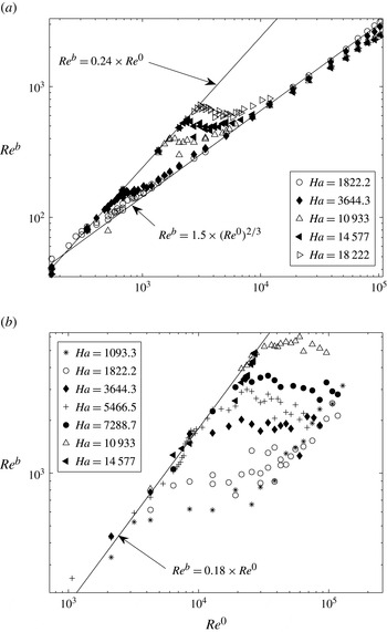
Graphs of
 $\mathit{Re}^{b}$
versus
 $\mathit{Re}^{0}$
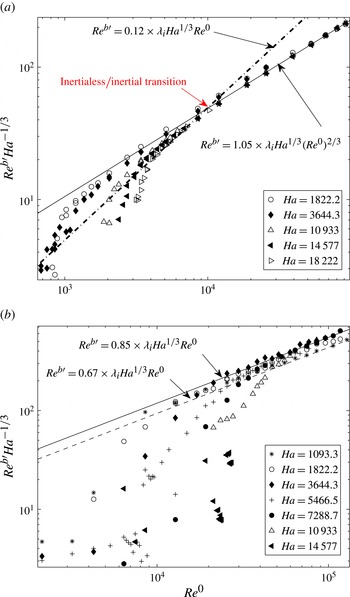
representing the average flow near the bottom wall for measurements spanning the whole range of parameters accessible in the experiment: (a)
 ${\it\lambda}_{i}=0.1$
; (b)
 ${\it\lambda}_{i}=0.3$
. Solid lines represent scaling laws for the inertialess regime of the form (3.16) and purely inertial regime (3.19).

For a spacing between probes of 2.5 mm in (2.1), instantaneous velocities can be measured locally to a precision of
 $1.6\ \text{mm}\ \text{s}^{-1}$
(at
 $B=0.5\ \text{T}/\mathit{Ha}=1822.2$
) down to
 $0.16\ \text{mm}\ \text{s}^{-1}$
(at
 $B=5\ \text{T}/\mathit{Ha}=18\,222$
). In the turbulent regimes considered in this paper, this provides a relative precision of at worse 5–0.5 %. These figures are considerably improved for averaged and RMS quantities, which are calculated over time series of typically
 $10^{5}$
samples.
4.2. Inertialess versus inertial three-dimensionality
4.2.1. Average flow
Figure 4 shows graphs of
 $\mathit{Re}^{b}$
against
 $\mathit{Re}^{0}$
over the full range of parameters spanned in our measurements for
 ${\it\lambda}_{i}=0.1$
and
 ${\it\lambda}_{i}=0.3$
. For any fixed value of
 $\mathit{Ha}$
, two regimes clearly stand out and data obtained at different values of
 $\mathit{Ha}$
all closely collapse into two single curves respectively for lower and higher values of
 $\mathit{Re}^{0}$
. For
 ${\it\lambda}_{i}=0.1$
, these curves follow the scalings
 $$\begin{eqnarray}\displaystyle & \mathit{Re}^{b}\simeq 0.24\mathit{Re}^{0}\quad \text{at small }\mathit{Re}^{0}, & \displaystyle\end{eqnarray}$$
 $$\begin{eqnarray}\displaystyle & \mathit{Re}^{b}\simeq 1.5(\mathit{Re}^{0})^{2/3}\quad \text{at large }\mathit{Re}^{0}. & \displaystyle\end{eqnarray}$$
The scaling at low
 $\mathit{Re}^{0}$
is found exclusively in the steady state, where vortices are mostly axisymmetric, and therefore subject to little inertia. It matches the scaling which characterises the inertialess regime (3.16) with
 $C_{0}\simeq 0.24$
, which suggests that no three-dimensionality driven by inertia is present there. Furthermore, from previous observations of flow patterns (Klein & Pothérat Reference Klein and Pothérat2010), the reason why this scaling holds at high
 $\mathit{Ha}$
is rather that the flow is indeed close to quasi two-dimensionality (typically
 $\mathit{Ha}>7500$
for
 ${\it\lambda}_{i}=0.1$
and
 $\mathit{Ha}>4000$
for
 ${\it\lambda}_{i}=0.3$
). At low
 $\mathit{Ha}$
, on the other hand, three-dimensionality was visible in the base flow, under the form of differential rotation affecting the base vortices. In this case, the validity of (4.5) indicates that this effect is driven by viscous friction.
When the flow becomes unsteady, inertia triggers a transition away from the inertialess regime (the conditions of this transition where analysed by Klein & Pothérat (Reference Klein and Pothérat2010) and earlier by Sommeria (Reference Sommeria1988) in the quasi-two-dimensional regime). Viscous effects are however still present and a purely inertial regime, in the sense that inertia-driven three-dimensionality dominates, is only reached asymptotically at high
 $\mathit{Re}^{0}$
, when the flow is turbulent. Then
 $\mathit{Re}^{b}$
tends to (4.6), which matches (3.19) with
 $C_{b}^{(N)}=1.5$
. For higher
 $\mathit{Ha}$
, the asymptotic value of
 $\mathit{Re}^{b}$
consistently stands slightly under that of (4.6), as predicted theoretically in (3.25). The correction factor due to the influence of the top wall is however weak, of the order of
 $f(N_{t})^{-2/3}\sim N_{t}^{0.08\pm 0.01}$
. Overall, the validity of generic scaling (3.19) for the average flow is verified over a wide range both of
 $\mathit{Re}^{0}$
and
 $\mathit{Ha}$
.
We were also able to verify that (3.16) still holds when the forcing scale
 ${\it\lambda}_{i}$
is varied, even though
 $C_{0}$
is slightly smaller for
 ${\it\lambda}_{i}=0.3$
than for
 ${\it\lambda}_{i}=0.1$
(
 $C_{0}\simeq 0.18$
versus
 $C_{0}\simeq 0.24$
). This point is mostly experiment-specific, as larger vortices are indeed more sensitive to friction from the side walls because a larger proportion of the lattice is in direct contact with them. Note that the values of
 $\mathit{Re}^{0}$
reached in the experiment for
 ${\it\lambda}_{i}=0.3$
are not large enough for the average flow to reach a fully developed inertial regime so we could not verify whether (3.19) was independent of
 ${\it\lambda}_{i}$
for the average flow.
4.2.2. Turbulent fluctuations
For
 ${\it\lambda}_{i}=0.1$
, fluctuations
 $U_{b}^{\prime }$
also exhibit two distinct regimes at low and high
 $\mathit{Re}$
. In the limit
 $\mathit{Re}^{0}\rightarrow \infty$
, they follow a unique law of the form
 $\mathit{Re}^{b\prime }\simeq C_{b}^{\prime }{\it\lambda}_{i}(\mathit{Re}^{0})^{2/3}\mathit{Ha}^{1/3}$
, with
 $C_{b}^{\prime }\simeq 1.05$
. This law is satisfied to a remarkable precision as soon as the flow is sufficiently turbulent (see figure 5
a). Experimental data shows the scaling
 ${\it\lambda}_{i}\mathit{Ha}^{1/3}$
to represent the ratio of velocity fluctuations relative to the mean flow in the limit of large Reynolds numbers (see Appendix(a)). Beyond the prefactor in
 ${\it\lambda}_{i}\mathit{Ha}^{1/3}$
, it remains that
 $\mathit{Re}^{b\prime }\sim (\mathit{Re}^{0})^{2/3}$
, which is of the form of (3.19), and therefore indicates that fluctuating structures are three-dimensional as a result of the inertial mechanism identified in § 3.3. As for the average flow, the validity of (3.19) is verified over a wide range of
 $\mathit{Re}^{0}$
and
 $\mathit{Ha}$
for turbulent fluctuations too.
Graphs of
 $\mathit{Re}^{b\prime }\mathit{Ha}^{-1/3}$
versus
 $\mathit{Re}^{0}$
, representing the RMS of velocity fluctuations near the bottom wall, for (a)
 ${\it\lambda}_{i}=0.1$
and (b)
 ${\it\lambda}_{i}=0.3$
. Solid and dashed lines represent scaling laws for the purely inertial regime (3.19).

At lower
 $\mathit{Re}$
, and for
 $\mathit{Ha}=18\,222$
only,
 $\mathit{Re}^{b\prime }$
scales as
 $\mathit{Re}^{b\prime }\simeq 0.12{\it\lambda}_{i}\mathit{Ha}^{1/3}\mathit{Re}^{0}$
, which is of the form (3.16) expected in the inertialess limit. Equations (3.16) and (3.19) intersect at
 $\mathit{Re}^{b\prime }\simeq 1.27\times 10^{3}$
. This point marks a form of transition between the inertialess regime and the regime of inertia-driven three-dimensionality. This transition occurs at a rather high value of the true interaction parameter
 $N_{t}^{\prime }$
based on
 $U_{b}^{\prime }$
, of the order of 26. Nevertheless a more precise estimate of this value, and a confirmation of its validity in the limit
 $\mathit{Ha}\rightarrow \infty$
would require further experiments at significantly higher magnetic fields. For
 $\mathit{Ha}<18\,222$
, the inertialess limit is not well achieved and this transition is therefore not as clear. Remarkably, since the inertialess regime for the average flow is only reached in the steady state, the inertialess regime for turbulent fluctuations corresponds to a state where inertia-driven three-dimensionality is present in the base flow but not in the turbulent fluctuations.
Equation (3.19) further remains valid for fluctuations when the injection scale varies albeit with a slightly lower value of constant
 $C_{b}^{\prime }$
(0.85 versus 1.05, see figure 5) due to the greater influence of the side walls at higher
 ${\it\lambda}_{i}$
. Fluctuations at
 ${\it\lambda}_{i}=0.3$
further reveal how these scalings degenerate at low
 $\mathit{Ha}$
: the asymptotic law (in the limit
 $\mathit{Re}^{0}\rightarrow \infty$
) stands a little lower than for higher
 $\mathit{Ha}$
(
 $C_{b}^{\prime }=0.67$
). This value of
 $C_{b}^{\prime }$
reflects a non-asymptotic dependence on
 $\mathit{Ha}$
: the scaling
 $U_{b}^{\prime }/U_{b}\sim {\it\lambda}_{i}\mathit{Ha}^{1/3}$
is indeed only valid in the limit
 $\mathit{Ha}\rightarrow \infty$
but not in the limit
 $\mathit{Ha}\rightarrow 0$
, where non-MHD turbulence still sustains strong fluctuations.
4.3. Measure of three-dimensionality at the wall where no forcing is applied
Now that regimes of quasi-two dimensionality, inertialess and purely inertial three dimensionality are identified, we shall examine the flow in the vicinity of the upper Hartmann wall to obtain a first quantification of three-dimensionality within these regimes. This shall be achieved by seeking the conditions in which the current injected at the bottom Hartmann wall feeds into the Hartmann layers near the top walls (when
 $l_{z}\gtrsim h$
and
 $l_{z}\gg h$
according to the theory from § 3.4), and by quantifying
 $l_{z}$
(§ 5).
4.3.1. Average flow
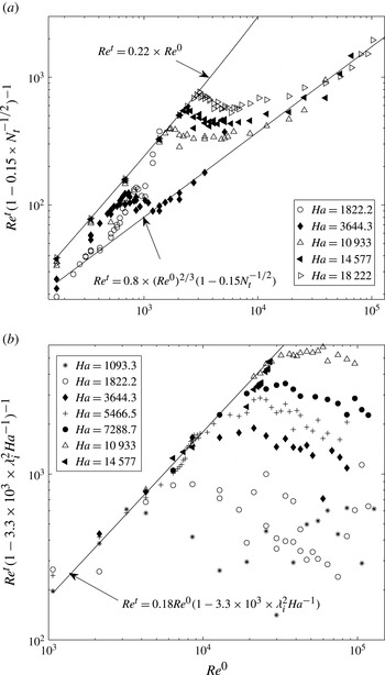
The variations of
 $\mathit{Re}^{t}$
with
 $\mathit{Re}^{0}$
are shown in figure 6 for
 ${\it\lambda}_{i}=0.1$
and
 ${\it\lambda}_{i}=0.3$
. Their general aspect is somewhat similar to those of
 $\mathit{Re}^{b}$
with
 $\mathit{Re}^{0}$
(figure 4), with a linear law in the inertialess regime (for
 $\mathit{Re}^{0}<Re_{I}^{0}$
), and a scaling of the form
 $\mathit{Re}^{t}\sim (\mathit{Re}^{0})^{2/3}$
in the purely inertial regime (for
 $\mathit{Re}^{0}$
sufficiently large). There are, however, two major differences. Firstly, in the inertialess regime, a dependence on
 $\mathit{Ha}$
of the form (3.22) is present (with
 $C_{t}^{0}=0.22$
versus
 $C_{b}^{0}=0.24$
for
 ${\it\lambda}_{i}=0.1$
, and
 $C_{t}^{0}=0.18\simeq C_{b}^{0}$
for
 ${\it\lambda}_{i}=0.3$
). The graph for
 ${\it\lambda}_{i}=0.3$
was scaled to find an estimate for the second constant in (3.22),
 $D_{t}^{(\mathit{Ha})}\simeq 3.10^{3}$
. The fact that flow intensities near top and bottom walls are close at high
 $\mathit{Ha}$
reflects that the average flow becomes quasi-two dimensional in the limit
 $\mathit{Ha}\rightarrow \infty$
. At lower
 $\mathit{Ha}$
, the validity of (3.22) indicates that the average flow looses intensity away from the bottom wall under the effect of viscous friction. The second important difference between the variations of
 $\mathit{Re}^{t}$
and
 $\mathit{Re}^{b}$
is visible on the graph for
 ${\it\lambda}_{i}=0.1$
: in the inertial regime too,
 $\mathit{Re}^{t}$
depends on
 $\mathit{Ha}$
, but this time according to scaling (3.26), which incorporates a correction for inertial effects in the presence of the top wall. Together with the validity of (3.22) in the range of lower
 $\mathit{Re}^{0}$
, This suggests that the upper wall actively influences the flow according to the mechanism outlined in § 3.4, where part of the current injected near the bottom wall was concentrated in the top Hartmann layer.
Graphs of
 $\mathit{Re}^{t}$
versus
 $\mathit{Re}^{0}$
, for (a)
 ${\it\lambda}_{i}=0.1$
and (b)
 ${\it\lambda}_{i}=0.3$
. (a) Curves are scaled by
 $(1-0.15\times N_{t}^{-1/2})^{-1}$
to show that all curves collapse into a scaling of the form (3.26) in the high
 $\mathit{Re}^{0}$
range. A similar collapse happens at low
 $\mathit{Re}^{0}$
for scaling (3.22) (not represented here for concision). (b) Curves are scaled by
 $(1-3.3\times 10^{3}\times {\it\lambda}_{i}^{2}\mathit{Ha}^{-1})^{-1}$
to show that all curves collapse into a scaling of the form (3.22). Values of
 $\mathit{Re}^{0}$
accessible in the experiment were not large enough to verify inertial scaling (3.26) at
 ${\it\lambda}_{i}=0.3$
.

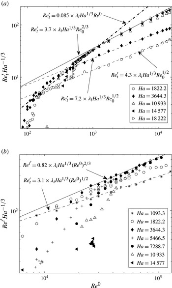
Graphs of
 $\mathit{Re}^{t\prime }\mathit{Ha}^{-1/3}$
versus
 $\mathit{Re}^{0}$
, for (a)
 ${\it\lambda}_{i}=0.1$
and (b)
 ${\it\lambda}_{i}=0.3$
. Scalings laws corresponding to the purely inertial regime are represented by solid and dashed-dotted lines when the top wall influences the flow (
 $l_{z}^{\prime (N)}\gtrsim h$
or
 $l_{z}^{\prime (N)}\gg h$
, scalings (3.22) and (3.26)) and by dashed lines when it does not
 $l_{z}^{\prime (N)}<h$
, scaling of the form (3.20).

4.3.2. Turbulent fluctuations
As for the average flow, the variations of the intensity of flow fluctuations near the top wall with
 $\mathit{Re}^{0}$
, reported in figure 7, resemble their counterpart near the bottom wall but exhibit a non-asymptotic behaviour at low
 $\mathit{Ha}$
. In the limit of large
 $\mathit{Ha}$
,
 $\mathit{Re}^{t\prime }$
clearly follows: (i) an inertialess regime at intermediate
 $\mathit{Re}^{0}$
and (ii) an inertia-driven three-dimensional one in the limit
 $\mathit{Re}^{0}\rightarrow \infty$
. These regimes are respectively characterised by scalings of the form
 $\mathit{Re}^{t\prime }\simeq C_{t}^{0\prime }{\it\lambda}_{i}\mathit{Re}^{0}\mathit{Ha}^{1/3}$
and
 $\mathit{Re}^{t\prime }\simeq C_{t}^{\prime }{\it\lambda}_{i}(\mathit{Re}^{0})^{2/3}\mathit{Ha}^{1/3}$
, which only differ from the scalings for
 $\mathit{Re}^{b\prime }$
through slightly lower values of
 $C_{t}^{0\prime }$
(0.085 versus
 $C_{b}^{0\prime }=0.12$
) and
 $C_{t}^{\prime }$
(0.88 versus
 $C_{b}^{\prime }=1.05$
). The slight differences in the first set of constants confirm that three-dimensionality driven by viscous effects is present in the inertialess regime. The most remarkable property of fluctuations near the top plate is that unlike for the base flow, the scaling exponent of
 $\mathit{Re}^{0}$
in the law
 $\mathit{Re}^{t\prime }(\mathit{Re}^{0})$
is different at low
 $\mathit{Ha}$
than in the limit of high
 $\mathit{Ha}$
. At low
 $\mathit{Ha}$
, it is indeed of the form
 $\mathit{Re}^{t}\simeq C_{t}^{\prime }(\mathit{Ha}){\it\lambda}_{i}\mathit{Ha}^{1/3}(\mathit{Re}^{0})^{1/2}$
. This phenomenon is clearly identifiable over one to two decades of
 $\mathit{Re}^{0}$
at
 ${\it\lambda}_{i}=0.1$
for
 $\mathit{Ha}\leqslant 3644.3$
, and at
 ${\it\lambda}_{i}=0.3$
for
 $\mathit{Ha}<1822.2$
. The corresponding flow fluctuations are of much lower intensity than predicted by any of the scenarii of § 3.4 involving an active influence of the top wall on the flow, so one can infer that the electrically driven flow does not reach the upper wall (i.e.
 $l_{z}^{\prime (N)}<h$
, where
 $l_{z}^{\prime (N)}$
is built on
 $U_{b}^{\prime }$
instead of
 $U_{b}$
). Instead, the exponent
 ${\textstyle \frac{1}{2}}$
of
 $\mathit{Re}^{b\prime }$
is the same as in scaling (3.20), found by Duran-Matute et al. (Reference Duran-Matute, Trieling and van Heijst2010) in a non-MHD inertial regime. It can be understood as follows: for the lowest values of
 $\mathit{Ha}$
, the flow near the bottom wall is entrained over a height
 $l_{z}^{(N)}<h$
(given by (3.17)) and so the scaling law (3.16) for
 $\mathit{Re}^{b}$
still holds. Fluctuations, by contrast, are not directly driven by current injection but receive energy from the average flow by inertial transfer. Furthermore, the non-asymptotic behaviour of
 $\mathit{Re}^{b\prime }$
, visible at low
 $\mathit{Ha}$
in figure 5(b), suggests that for such structures, the core current density becomes comparable to that through the bottom Hartmann layer. (This electric ‘leak’ from the bottom Hartmann layer explains the lower intensity of the fluctuations.) Consequently, fluctuations are powered by inertial transfer over the whole height
 $l_{z}^{\prime (N)}$
of the fluid layer where current passes. The Lorentz force balances inertia there, and is of order
 ${\it\sigma}B^{2}U_{c}^{\prime }$
. This phenomenology was noted in § 4.2 to translate into a fluctuating velocity in the core
 $U_{c}^{\prime }$
scaling as
 $(\mathit{Re}^{0})^{1/2}$
. The flow in the top region
 $l_{z}^{\prime (N)}\leqslant z\leqslant h$
, is thus not connected to the flow in the region
 $0\leqslant z\leqslant l_{z}^{\prime (N)}$
by eddy currents. Instead, it is entrained by viscous friction acting though a fluid thickness of
 $h-l_{z}^{\prime (N)}$
(figure 3
a). Therefore,
 $U_{t}^{\prime }$
is proportional to
 $U_{c}^{\prime }$
and decreases with
 $h-l_{z}^{\prime (N)}$
. This explains that
 $\mathit{Re}^{t\prime }\sim (\mathit{Re}^{0})^{1/2}$
. Since the thickness of the top region
 $h-l_{z}^{\prime (N)}$
decreases with
 $\mathit{Ha}$
, it also explains that at low
 $\mathit{Ha}$
, velocity fluctuations decrease faster when
 $\mathit{Ha}$
decreases, than at high
 $\mathit{Ha}$
, where they scale as
 $\mathit{Ha}^{1/3}$
(see Appendix(b)).
5. Symmetric, asymmetric three-dimensionalities and experimental measure of the Lorentz force diffusion length
From the characterisation of the flow near the wall where no forcing was applied, three-dimensionality was measured and its driving mechanisms identified. We shall now inspect electric potentials along the side walls to determine
 $l_{z}^{(N)}$
and
 $l_{z}^{\prime (N)}$
, where
 $l_{z}^{(N)}$
and
 $l_{z}^{\prime (N)}$
are respectively built on average and fluctuating quantities. This shall lead us to examine the trace of the forcing in the bulk of the flow, by tracking symmetric and antisymmetric three-dimensionality.
5.1. Interpretation of electric potential profiles along Shercliff walls
Unlike Hartmann layers, Shercliff layers, which develop along walls parallel to the magnetic field, do not possess a property providing a simple relation between electric potential at the side wall
 ${\it\phi}_{S}$
and velocities in the core (such as (2.2)) and so there is no simple way to deduct velocity variations along
 $\boldsymbol{B}$
from time series of non-intrusive measurements of electric potential at the wall. Furthermore, Shercliff layers are intrinsically three-dimensional because they result from a balance between the Lorentz force and horizontal viscous friction, which, as in the mechanisms responsible for three-dimensionality in the core, draws a horizontal current from the core into them. Nevertheless, if three-dimensionality is present in the core, then the current drawn from it into the Shercliff layers depends on
 $z$
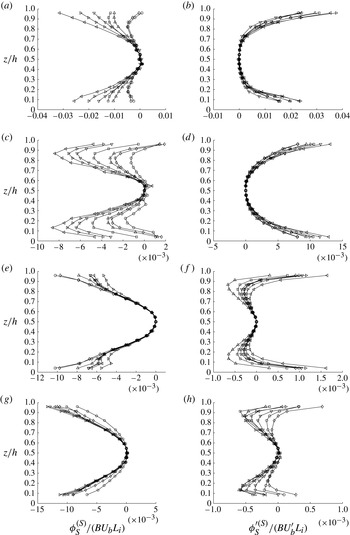
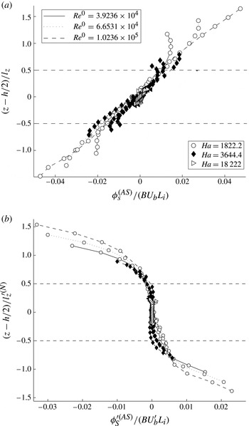
. More specifically, the asymmetric three-dimensionality in the core described in § 3.5 translates into an antisymmetric component of the profile of
 ${\it\phi}_{S}(z)$
of order at least
 $z^{3}$
(see Appendix(c)). Similarly, symmetric three-dimensionality in the core leads to a symmetric deformation of
 ${\it\phi}_{S}(z)$
. The reverse, however is not true, since even in quasi-two-dimensional flows, intrinsic three-dimensionality within the Shercliff layers induces a symmetric three-dimensional component in
 ${\it\phi}_{S}(z)$
(see, for example, Moreau Reference Moreau1990). Nevertheless, since this deformation is driven by linear viscous friction, it must depend linearly on the flow intensity, as measured by
 $U_{b}$
. Consequently, symmetric three-dimensionality in the core can still be detected by tracking nonlinear deformations of the symmetric part of the average of
 ${\it\phi}_{S}(z)/(BU_{b}L_{i})$
, and of the RMS of
 ${\it\phi}_{S}^{\prime }(z)/(BU_{b}^{\prime }L_{i})$
with
 $\mathit{Re}^{0}$
. The distinction between symmetric and asymmetric three-dimensionality is particularly important in our experiment where current is injected at one wall only: because of this particularity, asymmetric three-dimensionality gives a measure of the influence of the forcing on the flow dynamics.
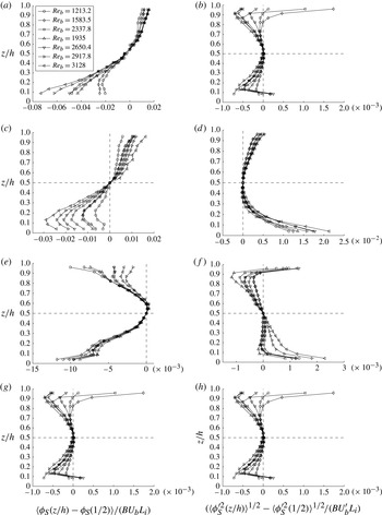
Profiles of
 $\langle {\it\phi}_{S}(z/h)-{\it\phi}_{S}(z/h={\textstyle \frac{1}{2}})\rangle$
(a,c,e,g), and
 $\langle {\it\phi}_{S}^{\prime }(z/h)^{2}\rangle ^{1/2}-\langle {\it\phi}_{S}^{\prime }(z/h={\textstyle \frac{1}{2}})^{2}\rangle ^{1/2}$
(b,d,f,h) measured at
 $(x,y)/L=(-0.5,0.24)$
: (a,b)
 $\mathit{Ha}=1822.2$
, (c,d)
 $\mathit{Ha}=3644.3$
, (e,f)
 $\mathit{Ha}=10\,933$
, (g,h)
 $\mathit{Ha}=18\,222$
.

Symmetric parts (superscript
 $S$
)
 ${\it\phi}_{S}^{(S)}$
and
 ${\it\phi}_{S}^{\prime (S)}$
respectively of
 $\langle {\it\phi}_{S}(z/h)-{\it\phi}_{S}(z/h={\textstyle \frac{1}{2}})\rangle$
(a,c,e,g), and of
 $\langle {\it\phi}_{S}^{\prime }(z/h)^{2}\rangle ^{1/2}-\langle {\it\phi}_{S}^{\prime }(z/h={\textstyle \frac{1}{2}})\rangle ^{1/2}$
(b,d,f,h), measured at
 $(x/L,y/L)=(-0.5,0.24)$
: (a,b)
 $\mathit{Ha}=1822.2$
, (c,d)
 $\mathit{Ha}=3644.3$
, (e,f)
 $\mathit{Ha}=10\,933$
, (g,h)
 $\mathit{Ha}=18\,222$
, legend is in figure 8.

Our analysis will be restricted to the turbulent regimes, where the flow and the signals are more intense and the corresponding measurements more precise. Since we consider variations of voltage with respect to the centrepoint of the vertical profile, the loss in precision on
 $\boldsymbol{{\rm\nabla}}{\it\phi}$
incurred by the lower flow intensity is compensated by the larger distance between electrodes, which is proportional to the amplitude of the signal (4–46 mm versus 2.5 mm for gradients of potentials measured in the central square of the Hartmann walls). For sufficiently turbulent flows, the precision on
 $\boldsymbol{{\rm\nabla}}{\it\phi}$
therefore remains similar to that of measurements along Hartmann walls. Profiles are chosen at
 $(x/h,y/h)=(-0.5,0.24)$
and for
 ${\it\lambda}_{i}=0.1$
only, but are representative of the phenomenology observed in other cases.
5.2. Symmetric versus antisymmetric three-dimensionality: influence of the forcing
Figure 8 shows the profiles of
 $\langle {\it\phi}_{S}(z/h)-{\it\phi}_{S}({\textstyle \frac{1}{2}})\rangle$
and
 $\langle {\it\phi}_{S}(z/h)^{\prime 2}\rangle ^{1/2}-\langle {\it\phi}_{S}({\textstyle \frac{1}{2}})^{\prime 2}\rangle ^{1/2}$
for the same set of values of
 $\mathit{Re}^{0}$
, at different
 $\mathit{Ha}$
. They are respectively normalised by
 $BU_{b}L_{i}$
and
 $BU_{b}^{\prime }L_{i}$
. First, the amplitude of the variations of both these quantities decreases by about an order of magnitude between
 $\mathit{Ha}=1822.2$
and
 $\mathit{Ha}=18\,222$
: the flow becomes closer to quasi-two dimensionality as
 $\mathit{Ha}$
increases and the proportion of current that transits from the core to the Shercliff layers reduces correspondingly. Second, all graphs show that the vertical gradient of these quantities increases with
 $\mathit{Re}^{0}$
. This is due to the increasing amount of current drawn into the core by inertial effects, which loops back through the Shercliff layers. This effect being nonlinear, it can be measured on the graphs through the discrepancy between curves at different values of
 $\mathit{Re}^{0}$
for the same
 $\mathit{Ha}$
. At
 $\mathit{Ha}=1822.2$
, the eddy currents originating from the core are strongly concentrated near the bottom wall and practically zero near the top wall (this is even more spectacular on the profiles of fluctuations). Together with the scaling
 $\mathit{Re}_{t}^{\prime }\sim (\mathit{Re}^{0})^{1/2}$
observed in this regime (§ 4.3), this concurs to show that the top wall is not active and that
 $l_{z}^{\prime (N)}<h$
. The phenomenology is similar at
 $\mathit{Ha}=3644.3$
, except for a slight gradient in the vicinity of the top wall, suggesting that
 $l_{z}^{\prime (N)}$
is closer to
 $h$
and that eddy currents already appear between the core and the top Hartmann layer. At the two highest values of
 $\mathit{Ha}$
, the profiles of both averages and fluctuations become more symmetric, to be almost symmetric at
 $\mathit{Ha}=18\,222$
, but with an important difference between them. All average profiles converge towards a single curve at high
 $\mathit{Re}^{0}$
: this indicates linearity with the flow intensity and therefore suggests that the corresponding three-dimensionality is due to the viscous effects in the Shercliff layers. By contrast, the profiles of fluctuations are more scattered: although the amplitude of the corresponding currents is quite weak, this nonlinearity suggests the presence of symmetric three-dimensionality in turbulent fluctuations, as theorised in § 3.5.
Symmetric three-dimensionality can be more precisely traced by inspecting the symmetric parts
 ${\it\phi}_{S}^{(S)}$
and
 ${\it\phi}_{S}^{\prime (S)}$
of the profiles of
 $\langle {\it\phi}_{S}(z/h)-{\it\phi}_{S}({\textstyle \frac{1}{2}})\rangle$
and
 $\langle {\it\phi}_{S}(z/h)^{\prime 2}\rangle ^{1/2}-\langle {\it\phi}_{S}({\textstyle \frac{1}{2}})^{\prime 2}\rangle ^{1/2}$
, in figure 9. While inertia-driven, symmetric three-dimensionality is practically absent from fluctuations at low
 $\mathit{Ha}$
, it becomes dominant a large
 $\mathit{Ha}$
. The average flow, by contrast, exhibits the opposite behaviour, with inertia-driven symmetric three-dimensionality absent at high Hartmann number. Since the profiles of fluctuations are highly symmetric in this regime, this important difference shows that at
 $\mathit{Ha}>10\,933$
, where
 ${\it\tau}_{2D}$
becomes shorter than the turnover time for the large scales
 ${\it\tau}_{u^{\prime }}$
(or, equivalently, when
 $N_{t}$
becomes greater than unity), the asymmetry induced by the forcing is mostly confined to the base flow and the Lorentz force damps it out before it is transferred to turbulent fluctuations. The dimensionality of turbulent fluctuations generated in this regime is therefore subject to little influence from the inhomogeneity of the forcing.
Antisymmetric part (superscript (
 $AS$
))
 ${\it\phi}_{S}^{(AS)}$
and
 ${\it\phi}_{S}^{\prime (AS)}$
respectively of the profiles of (a)
 $\langle {\it\phi}_{S}(z/h)-{\it\phi}_{S}({\textstyle \frac{1}{2}})\rangle$
and (b)
 $\langle {\it\phi}_{S}^{\prime }(z/h)^{2}\rangle ^{1/2}-\langle {\it\phi}_{S}^{\prime }(z/h={\textstyle \frac{1}{2}})^{2}\rangle ^{1/2}$
, measured at
 $(x/L,y/L)=(-0.5,0.24)$
, with
 $(z-h/2)$
respectively normalised by
 $l_{z}^{(N)}$
and
 $l_{z}^{\prime (N)}$
(built on
 $U_{b}$
and
 $U_{b}^{\prime }$
). Profiles are plotted for
 ${\it\lambda}_{i}=0.1$
, for five values of
 $\mathit{Ha}$
and three values of
 $\mathit{Re}^{0}$
for each value of
 $\mathit{Ha}$
.

5.3. Experimental measure of the length of diffusion by the Lorentz force
We shall now extract the lengthscale of momentum diffusion by the Lorentz force
 $l_{z}^{(N)}(B,U_{b})$
, defined by (3.17) from the antisymmetric parts
 ${\it\phi}_{S}^{(AS)}$
and
 ${\it\phi}_{S}^{\prime (AS)}$
of the profiles of
 $\langle {\it\phi}_{S}(z/h)-{\it\phi}_{S}({\textstyle \frac{1}{2}})\rangle$
and
 $\langle {\it\phi}_{S}(z/h)^{\prime 2}\rangle ^{1/2}-\langle {\it\phi}_{S}({\textstyle \frac{1}{2}})^{\prime 2}\rangle ^{1/2}$
. Profiles of these quantities are plotted on figure 10 respectively against
 $(z-h/2)/l_{z}^{(N)}$
and
 $(z-h/2)/l_{z}^{\prime (N)}$
. With this choice of variables, since
 $l_{z}^{(N)}$
and
 $l_{z}^{\prime (N)}$
increase with
 $\mathit{Ha}$
, curves obtained at higher
 $\mathit{Ha}$
are shorter than those at low
 $\mathit{Ha}$
, and all curves are centred on zero. The first important result is that profiles of average and fluctuations collapse well into a single curve each: this indicates that the momentum forced near the bottom wall reaches into the flow over
 $l_{z}^{(N)}$
. This establishes the validity of scaling (3.17) for
 $l_{z}^{(N)}$
and
 $l_{z}^{\prime (N)}$
, for the average flow and the fluctuations, respectively.
The average potentials follow a linear profile, with strong discrepancies to it in regions where
 $|(z-h/2)/l_{z}^{(N)}|>0.5$
(marked by horizontal dashed lines). Only at
 $\mathit{Ha}=1822.2$
are these regions clearly reached, as
 $l_{z}^{(N)}$
is notably smaller than
 $h$
whereas at
 $\mathit{Ha}=3644.3$
,
 $l_{z}\simeq h$
, depending on
 $\mathit{Re}^{0}$
. Strong current exists in the corresponding regions of the core and so diffusion by the Lorentz force is not effective there. Since the inhomogeneity is asymmetric, it can be attributed to the forcing. In that sense, it carries the signature of the forcing dimensionality. In the region
 $|(z-h/2)/l_{z}^{(N)}|<0.5$
, by contrast, momentum diffusion by the Lorentz force dominates inertia: the (asymmetric) horizontally divergent current collapses in the core and therefore in the Shercliff layers, where it would normally return. For
 $\mathit{Ha}>3644.3$
,
 $l_{z}^{(N)}>h$
: discrepancies to linearity are less pronounced and reflect eddy currents more homogeneously spread along the height of the vessel. This phenomenology holds for both the average flow and the fluctuations but the collapse to a single curve is significantly better on the profiles of fluctuations. It is remarkable that the antisymmetric part of turbulent fluctuations in the region
 $|(z-h/2)/l_{z}^{\prime (N)}|<0.5$
is dominated by momentum diffusion by the Lorentz force, when at the same time, three-dimensionality can still be observed in the symmetric part of the profiles. Since for
 $\mathit{Ha}>10\,933$
, this region extends along the full height of the vessel, this implies that the three-dimensionality of turbulent fluctuations observed in this range of parameters (visible in particular on the symmetric profiles of figure 9) is not induced by the forcing, even though the forcing still induces some three-dimensionality in the average flow. This is the second important result of this section.
6. Weak versus strong three-dimensionality in unsteady regimes
6.1. Global quantification of weak and strong three-dimensionality
In §§ 3–5, the vertical profiles of electric potential and the scalings for
 $U_{b},U_{t},U_{b}^{\prime }$
and
 $U_{t}^{\prime }$
were shown to be efficient tools to detect three-dimensionality, and to contain the viscous or inertial signature of its origin. We shall now more precisely measure three-dimensionality and determine its nature by quantifying weak and strong three-dimensionalities, which we previously introduced in Klein & Pothérat (Reference Klein and Pothérat2010). In particular, we shall estimate the extent to which either form of three-dimensionality is eradicated in the quasi-two-dimensional limit.
Let us start by recalling that weak three-dimensionality is characterised by a variation in flow intensity between two-dimensional ‘slices’ of topologically equivalent flows in the
 $(x,y)$
plane. Strong three-dimensionality, by contrast, involves different profiles of physical quantities along
 $z$
at different locations
 $(x,y)$
. Following Klein & Pothérat (Reference Klein and Pothérat2010), their respective occurrence shall be quantified by comparing measurements at bottom and top Hartmann walls at
 $z=0$
and
 $z=h$
, by means of two types of correlations:
 $$\begin{eqnarray}\displaystyle & \displaystyle C_{1}^{\prime }(x,y)=\frac{\displaystyle \mathop{\sum }_{t=0}^{T}\partial _{y}{\it\phi}_{b}^{\prime }(x,y,t)\partial _{y}{\it\phi}_{t}^{\prime }(x,y,t)}{\displaystyle \sqrt{\mathop{\sum }_{t=0}^{T}\partial _{y}{{\it\phi}^{\prime }}_{b}^{2}(x,y,t)\mathop{\sum }_{t=0}^{T}\partial _{y}{{\it\phi}^{\prime }}_{t}^{2}(x,y,t)}}, & \displaystyle\end{eqnarray}$$
 $$\begin{eqnarray}\displaystyle & \displaystyle C_{2}^{\prime }(x,y)=\frac{\displaystyle \mathop{\sum }_{t=0}^{T}\partial _{y}{\it\phi}_{b}^{\prime }(x,y,t)\partial _{y}{\it\phi}_{t}^{\prime }(x,y,t)}{\displaystyle \mathop{\sum }_{t=0}^{T}\partial _{y}{{\it\phi}^{\prime }}_{b}^{2}(x,y,t)}, & \displaystyle\end{eqnarray}$$
 $T$
is the duration of the recorded signals. Values of
 $C_{1}^{\prime }$
depart from unity whenever strong three-dimensionality is present, but are unaffected by weak three-dimensionality.
 $C_{2}^{\prime }$
, on the other hand, differs from unity whenever either weak or strong three-dimensionality is present. In order to minimise the influence of the side walls, we shall reason on the spatial averages
 $\overline{C_{i}^{\prime }}$
and
 $1-\overline{C_{i}^{\prime }}$
of
 $C_{i}^{\prime }$
and
 $1-C_{i}^{\prime }$
over the central square region (see § 2). Whilst
 $1-C_{1}^{\prime }$
and
 $1-C_{2}^{\prime }$
give a measure of three-dimensionalities,
 $C_{1}^{\prime }$
and
 $C_{2}^{\prime }$
reflect the emergence of two-dimensionality, respectively in the strong sense, and in both the weak and the strong sense. A minor limitation of this method, however, is that fluctuations that remain at all time symmetric with respect to the vessel mid-plane (
 $z/h={\textstyle \frac{1}{2}}$
) cannot be detected as they do not affect the values of
 $C_{1}^{\prime }$
nor
 $C_{2}^{\prime }$
. Fluctuations that are symmetric on average but not at all time, such as those detected in the symmetric part of
 ${\it\phi}_{S}^{\prime }$
(§ 5), may, by contrast, alter the values of the correlations. While the former type of fluctuation is unlikely to generate strong three-dimensionality, the latter is the most likely form of strong symmetric three-dimensionality, since it results from randomly localised three-dimensional disturbances, which are unaffected by the asymmetry of the forcing and therefore distributed symmetrically along the vessel height. The experimental precision on
 $\overline{C_{i}^{\prime }}$
can be estimated from the ratio of signal amplitude to uncorrelated noise. Using definitions (6.1) and (6.2), we find that the relative theoretical precision is never worse than 2 %. It concerns regimes of low
 $\mathit{Ha}$
were the signal is lower and the values of
 $\overline{C_{i}^{\prime }}$
are close to zero. For the highest values of
 $\mathit{Ha}$
, where
 $\overline{C_{i}^{\prime }}$
becomes very close to one, the uncertainty falls around that incurred by the mechanical tolerances of the vessel (approximately 0.1 %). In practise, we found it to be around 0.5 %.
(a) Correlations and (b) co-correlations of electric potential gradient between bottom and top Hartmann walls, averaged over the central square. Data were obtained from measurements both with
 ${\it\lambda}_{i}=0.1$
and
 ${\it\lambda}_{i}=0.3$
. (c) Snapshots of contours of electric potential taken for four values of
 $N_{t}^{\prime }$
and examples of spectra taken pairs of probes within the central square respectively from top (green, lower curve) and bottom plate (red, upper curve), at the same point
 $(x,y)$
.

We plot
 $\overline{C_{i}^{\prime }}$
and
 $1-\overline{C_{i}^{\prime }}$
in figure 11 against the true interaction parameter based on the velocity fluctuations and the injection scale
 $N_{t}^{\prime }(L_{i})=({\it\sigma}B^{2}L_{i}/{\it\rho}U_{b}^{\prime }){\it\lambda}_{i}^{-2}$
. All our measurement points collapse into two single curves
 $\overline{C_{1}^{\prime }}(N_{t})$
and
 $\overline{C_{2}^{\prime }}(N_{t})$
, indicating that three-dimensionality in the fluctuations is exclusively of inertial nature. This is consistent with the scalings found for fluctuations
 $U_{b}^{\prime }$
and
 $U_{t}^{\prime }$
in § 4, which reflected the presence of inertia in the core too. In the limit
 $N_{t}^{\prime }\rightarrow \infty$
, both types of correlations become close to one within a precision of approximately 1 %, indicating that in these regimes, the flow is very close to quasi-two-dimensionality. Furthermore, in the limit
 $N_{t}^{\prime }\rightarrow \infty$
,
 $1-\overline{C_{1}^{\prime }}(N_{t})\sim N_{t}^{\prime -0.9}$
and
 $1-\overline{C_{2}^{\prime }}(N_{t})\sim N_{t}^{\prime -0.9}$
, up to the point where these quantities reach a plateau reflecting the level of signal noise. In fact two such plateaux shoot off from the main
 $N_{t}^{\prime -0.9}$
law, that correspond to the two different levels of signal to noise ratio for
 ${\it\lambda}_{i}=0.1$
and
 ${\it\lambda}_{i}=0.3$
. Despite their purely empirical nature, these scalings give a strong experimental evidence that the flow becomes asymptotically quasi-two-dimensional and that a vanishingly small amount of three-dimensionality always remains present. By contrast, the transition between two- and three-dimensional states in MHD flows with non-dissipative boundaries (such as free-slip conditions studied by Thess & Zikanov (Reference Thess and Zikanov2007) or periodic boundary conditions by Zikanov & Thess (Reference Zikanov and Thess1998), Pothérat & Dymkou (Reference Pothérat and Dymkou2010)) occurred through bifurcations at a critical value of the parameter representing the flow intensity. This fundamental difference in behaviour must be attributed to the role of walls, in line with our recent theory (Pothérat Reference Pothérat2012) showing that walls incur weak three-dimensionality as soon as
 $N$
(or
 $N_{t}$
) is finite.
In the limit
 $N_{t}^{\prime }\rightarrow 0$
,
 $\overline{C_{1}^{\prime }}$
and
 $\overline{C_{2}^{\prime }}$
exhibit several noticeable differences. Firstly, measurements empirically obey two different scalings:
 $\overline{C_{1}^{\prime }}\sim N_{t}^{\prime 1/2}$
and
 $\overline{C_{2}^{\prime }}\sim N_{t}^{\prime }$
. This indicates that weak three-dimensionality is more significant than strong three-dimensionality. This effect is in part due to the nature of the forcing: for low magnetic fields and strong currents, electric currents remain in the vicinity of the bottom wall, where the flow is intensely stirred. By contrast, very little current flows near the top wall. Whatever weak flow remains there is mostly entrained by viscous momentum diffusion from the intense flow near the bottom wall. Both share the same large patterns, as on the snapshots of streamlines (a) and (b) from figure 11, and are therefore somewhat correlated in the weak sense. By contrast, the very small intensity of the flow near the top wall extinguishes correlation in the strong sense.
The power laws found in the limits
 $N_{t}^{\prime }\rightarrow 0$
and
 $N_{t}^{\prime }\rightarrow \infty$
intersect at
 $N_{t}^{\prime }=N_{t}^{\prime 2D}\simeq 4.5$
, and remain remarkably valid in their respective ranges
 $N_{t}^{\prime }<4.5$
and
 $N_{t}^{\prime }>4.5$
, In this sense, the value
 $N_{t}^{\prime 2D}$
marks a form of transition between quasi-two-dimensional and three-dimensional states. We insist, however, that this is not a critical value of
 $N_{t}^{\prime }$
since no bifurcation occurs in the flow states at this point. Also, it provides a rather global appraisal of the flow state but it is certainly not the case that for
 $N_{t}^{\prime }>4.5$
, every structure in the flow is quasi-two-dimensional.
6.2. Frequency dependence of strong three-dimensionality
We shall now seek to characterise three-dimensionality locally by analysing the frequency spectra from the fluctuations of
 $\boldsymbol{{\rm\nabla}}{\it\phi}$
near each of the Hartmann walls. In figure 11, pairs of such spectra are shown that were obtained from signals acquired at locations of either Hartmann walls exactly aligned with the magnetic field lines (i.e. respectively at
 $z=0$
and
 $z=h$
, but at the same coordinates
 $(x,y)$
). These were taken in the central square region, so as to minimise the influence of the side walls. At a sampling frequency of 128 Hz, signals would theoretically render fluctuations of up 64 Hz. To increase signal quality, however, we apply a low-pass filter at 45 Hz so as to avoid electromagnetic interferences from the mains. The physically relevant part of the spectra correspondingly extends approximately over 2–3 decades. For values of
 $N_{t}^{\prime }$
noticeably higher than 4.5, top and bottom spectra are practically identical, as would be expected of a flow that would be quasi-two-dimensional at all scales. Since spectra do not carry any phase information, however, identical spectra do not provide a proof that all scales are indeed quasi-two-dimensional, but merely that no obvious three-dimensionality is present at any scale. Pairs of spectra at lower values of
 $N_{t}^{\prime }$
, on the other hand, show a clear manifestation of three-dimensionality as fluctuations of higher frequency carry significantly less energy in the vicinity of the top wall than near the bottom wall. Fluctuations of lower frequency, by contrast, carry the same amount of energy. When
 $N_{t}^{\prime }$
is reduced, the range of frequencies affected by three-dimensionality widens to the low-frequency range and ends up contaminating the whole spectrum at the lowest values of
 $N_{t}^{\prime }$
. This qualitative comparison of spectra indicates that fluctuations of higher frequencies, and smaller scales by extension, are more sensitive to three-dimensionality than those of lower frequencies and larger scales, in accordance with Sommeria & Moreau (Reference Sommeria and Moreau1982)’s prediction. A closer inspection of superimposed spectra further suggests the existence of a cutoff frequency
 $f_{c}$
separating three-dimensional high-frequency fluctuations from lower-frequency fluctuations with the same amount of energy near both walls. It also appears that
 $f_{c}$
increases with
 $N_{t}^{\prime }$
. To quantify the behaviour of
 $f_{c}(N_{t}^{\prime })$
, we define a partial correlation function between signals on the bottom and top Hartmann walls in the strong sense:
 $$\begin{eqnarray}\displaystyle c_{1}^{\prime }(\,f)=\frac{\displaystyle \mathop{\sum }_{t=0}^{T}\mathscr{B}_{f}\partial _{y}{\it\phi}_{\text{b}}^{\prime }(t)\partial _{y}{\it\phi}_{\text{t}}^{\prime }(t)}{\displaystyle \sqrt{\mathop{\sum }_{t=0}^{T}\mathscr{B}_{f}\partial _{y}{{\it\phi}^{\prime }}_{\text{b}}^{2}(t)\displaystyle \mathop{\sum }_{t=0}^{T}\partial _{y}{{\it\phi}^{\prime }}_{\text{t}}^{2}(t)}}. & & \displaystyle\end{eqnarray}$$
The definition of
 $c_{1}^{\prime }(\,f)$
hardly differs from that of
 $C_{1}^{\prime }(\,f)$
, but for the fact that the full signal recorded from the bottom wall is replaced with a filtered counterpart, processed through an eighth-order low-pass filter of cutoff frequency
 $f$
, incurring neither phase nor amplitude distortion (denoted
 $\mathscr{B}_{f}$
). Figure 12 shows the typical variations of
 $c_{1}^{\prime }(\,f)$
when
 $f$
spans the whole part of the spectrum resolved in our measurements. Their most important feature is the presence of a maximum, which can be understood by considering two spectra obtained from top and bottom walls overlapping up to a frequency
 $f_{c}$
. Increasing
 $f$
from 0 for
 $f<f_{c}$
adds fluctuations to the bottom signal that are correlated with existing frequencies in the signal from the top wall, so
 $c_{1}^{\prime }(\,f)$
increases. When
 $f$
is increased beyond
 $f_{c}$
, the fluctuations added to the bottom signal are decorrelated from existing frequencies in the top one, so
 $c_{1}^{\prime }(\,f)$
decreases. The position of the maximum thus gives a good measure of
 $f_{c}$
. Note that the same approach cannot be applied to
 $C_{2}^{\prime }$
, as a partial correlation
 $c_{2}(\,f)^{\prime }$
obtained from
 $C_{2}^{\prime }$
by replacing the bottom signal by a filtered counterpart would diverge in the limit
 $f\rightarrow 0$
. This is because the filtered bottom signal vanishes in this limit (This feature is absent from the behaviour of
 $c_{1}(\,f)^{\prime }$
as signals are normalised by their intensity by construction). Nevertheless, from Sommeria & Moreau’s (Reference Sommeria and Moreau1982) theory, the existence of a cutoff lengthscale
 $k_{c}$
separating quasi-two-dimensional from three-dimensional structures stems from no assumption on the nature of inertial effects so it can be expected to exist both for weak and strong three-dimensionality. Yet, if instabilities occurred at the scale of individual structures, they would incur strong rather than weak three-dimensionality so in any case,
 $f_{c}$
is linked to the minimum size of structures that are stable to three-dimensional perturbations. The question of the nature of the possible instabilities that occur below this size remains to be clarified with dedicated analysis.
The variations of
 $f_{c}(N_{t}^{\prime })$
are represented on figure 13. Measurements points across the whole range of unsteady flows reachable in the experiment once again collapse into a single curve, so
 $f_{c}$
is determined by
 $N_{t}^{\prime }$
, as
 $\overline{C_{1}^{\prime }(\,f)}$
and
 $\overline{C_{2}^{\prime }(\,f)}$
were, with a scaling law
 $$\begin{eqnarray}f_{c}\backsimeq 1.7{\it\tau}_{u^{\prime }}^{-1}N_{t}^{0.67},\end{eqnarray}$$
where
 ${\it\tau}_{u^{\prime }}=L_{i}/U_{b}^{\prime }$
is the turnover time at the forcing scale. While this law is verified to a great precision for
 ${\it\lambda}_{i}=0.1$
(the exponent 0.67 is obtained to a precision of
 $\pm 0.03$
), a small departure to it is visible at low
 $N_{t}^{\prime }$
for
 ${\it\lambda}_{i}=0.3$
, that must be attributed to the greater influence of the walls. Indeed the large vortices forced in such regimes can be expected to induce local separations of the parallel boundary layers, acting as a source of instability that could lower
 $f_{c}$
. Unfortunately, our measurements do not allow us to test this hypothesis further. It is however consistent with the fact that boundary-layer separation is suppressed at higher
 $N_{t}^{\prime }$
(Pothérat et al.
Reference Pothérat, Sommeria and Moreau2005). The fact that this empirical scaling is reasonably independent of the forcing scale gives good evidence of its universality. This important result brings a phenomenological confirmation of Sommeria & Moreau’s (Reference Sommeria and Moreau1982) theory, even though (6.4) is not strictly equivalent to these authors’ scaling for a cutoff wavelength
 $k_{c}$
, of the form
 $k_{c}\sim N^{\prime 1/3}$
.
Variations of partial correlation
 $c_{1}^{\prime }(\,f)$
with the cutoff frequency of filter
 $\mathscr{B}_{f}$
applied to the signal measured at the bottom wall. Curves are obtained for
 ${\it\lambda}_{i}=0.1$
and
 $N_{t}^{\prime }=0.12$
for a pair of probes within the central square. Curves obtained for different parameters exhibit the same features. (a–d) Spectra of the filtered signals and top signals plotted in terms of the frequency normalised by the turnover frequency associated to RMS fluctuations
 ${\it\tau}_{u^{\prime }}^{-1}$
. Frequency
 $f_{c}$
is also represented.

Cut-off frequency
 $f_{c}$
, separating quasi-two-dimensional fluctuations from three-dimensional ones, normalised by
 ${\it\tau}_{u^{\prime }}^{-1}$
, the eddy turnover frequency built on
 $U_{b}^{\prime }$
, versus
 $N_{t}^{\prime }$
.

7. Conclusions
We have conducted a detailed analysis of the conditions of appearance of three-dimensionality in low-
 $\mathit{Rm}$
MHD turbulence in a channel bounded by two solid walls. We have clarified the mechanisms governing this phenomenon and were able to quantify it through the scaling of flow quantities. These results can be summarised as follows.
7.1. The force driving three-dimensionality determines the scalings for the Reynolds number near Hartmann walls
Three-dimensionality appears whenever viscous or inertial forces exist in the core of the flow, i.e. outside the Hartmann boundary layers. The nature of these forces was identified through scaling laws linking the total current injected to drive the flow and the velocities in the vicinity of the bottom wall (where the flow is forced by injecting electric current), and the top wall. Driving the flow in this way offers a convenient way of controlling the external force generating the flow. Scaling laws expressing the response of the flow to the forcing were written in terms of Reynolds numbers
 $\mathit{Re}^{b}$
,
 $\mathit{Re}^{t}$
, against the forcing intensity measured by
 $\mathit{Re}^{0}$
. These yield two conclusions regarding both the average flow and for turbulent fluctuations.
-
(i) Both quasi-two-dimensional flows and flows where three-dimensionality is driven by viscous friction in the core obey scaling laws of the form first put forward by Sommeria (Reference Sommeria1988):
$\mathit{Re}^{b}\sim \mathit{Re}^{0}$
. We gathered both in a regime which we called inertialess. -
(ii) For flows where three-dimensionality is purely driven by inertia, in particular turbulent ones,
$\mathit{Re}^{b}\sim (\mathit{Re}^{0})^{2/3}$
.


7.2. In a channel of height
$h$
, three-dimensionality is determined by the ratio of the length of diffusion of momentum by the Lorentz force
$l_{z}$
to
$h$


Momentum diffusion along
 $\boldsymbol{B}$
is opposed by either viscous or inertial forces and this determines the thickness
 $l_{z}$
of the fluid layer where momentum diffuses. If viscous effects oppose the Lorentz force, then
 $l_{z}\sim l_{\bot }Ha$
, whereas when inertia opposes it,
 $l_{z}\sim l_{\bot }N^{1/2}$
. For a channel of height
 $h$
, two regimes can be distinguished.
-
(i) If
$h<l_{z}$
, eddy currents flow in the top Hartmann layer and the upper wall is active in the sense that it strongly influences the flow.
$\mathit{Re}^{t}$
then scales as
$\mathit{Re}^{t}\sim \mathit{Re}^{0}(1-D^{(\mathit{Ha})}{\it\lambda}_{i}^{2}\mathit{Ha}^{-1})$
in the inertialess regime, and as
$\mathit{Re}^{t}\sim (\mathit{Re}^{0})^{2/3}(1-D^{(N)}N_{t}^{-1/2})$
in the inertial regime. The flow becomes quasi-two-dimensional in the limit
$l_{z}/h\rightarrow \infty$
. (When the top wall is active, but the flow is still three-dimensional, inertia also incurs a small correction to the law
$\mathit{Re}^{b}\sim (\mathit{Re}^{0})^{2/3}$
that further reduces
$\mathit{Re}^{b}$
slightly.) -
(ii) If
$h>l_{z}$
, momentum diffusion does not reach the top wall and only a weak residual flow exists there. In this sense the top wall is passive and the flow there satisfies the scaling found by Duran-Matute et al. (Reference Duran-Matute, Trieling and van Heijst2010) of
$\mathit{Re}^{t}\sim (\mathit{Re}^{0})^{1/2}$
.






These scalings were verified experimentally for two injection scales (
 ${\it\lambda}_{i}=0.1$
and 0.3),
 $1093.3\leqslant \mathit{Ha}\leqslant 18\,222$
and
 $\mathit{Re}^{0}$
up to
 $1.03\times 10^{5}$
, which corresponded to a Reynolds number based on turbulent fluctuations
 $\mathit{Re}^{b\prime }$
of up to approximately
 $6\times 10^{3}$
. Exponents in the scalings for Reynolds number near Hartmann walls are recovered both experimentally and from a generic theory so they may be deemed a universal feature of MHD turbulence in channels. The same may not hold true for the multiplicative constants, which can be expected to depend on the geometry of the forcing.
The average flow was found to be in the inertialess regime exclusively when the flow was steady and to exhibit inertia-driven three-dimensionality in the limit of
 $\mathit{Re}^{0}\rightarrow \infty$
. The fluctuating part of the unsteady flow, by contrast, exhibits a transition between the inertialess regime and the regime of inertial three-dimensionality. This difference between average and fluctuations singles out a range of forcing intensities where inertial three-dimensionality due to the forcing affects only the average flow but not turbulent fluctuations.
7.3. Three-dimensionality was observed independently of the dimensionality of the forcing
We were then able to track the three-dimensionality due to the electric forcing by separating symmetric and antisymmetric parts of profiles of electric potential measured along Shercliff walls. This led us to identify two basic features of low
 $\mathit{Rm}$
MHD turbulence.
-
(i) Diffusion of momentum by the Lorentz force is indeed effective over the length theorised by Sommeria & Moreau (Reference Sommeria and Moreau1982), which we showed to be rather precisely
$l_{z}\simeq N^{1/2}$
both for the average flow and for turbulent fluctuations. -
(ii) When
${\it\tau}_{2D}({\it\lambda}_{i})\lesssim {\it\tau}_{U}({\it\lambda}_{i})$
, the asymmetry between the top and bottom wall introduced by the forcing was dampened out during the energy transfer from the mean flow to the large turbulent scales. In this case, the trace of the forcing was mostly borne by the average flow. The features of the turbulence observed in the flow fluctuations are then reasonably independent of it. In this sense, the three-dimensionality observed in this regime is intrinsic and not induced by the forcing.


7.4. Three-dimensionality vanishes asymptotically in the quasi-two dimensional limit
Finally, in the turbulent regimes, we were able to quantify weak and strong three-dimensionalities, which we first introduced in Klein & Pothérat (Reference Klein and Pothérat2010), both globally and in a frequency analysis of the flow. This brought further clarification on the mechanisms driving three-dimensionality.
-
(i) The transition between the quasi-two-dimensional and three-dimensional states of wall-bounded MHD turbulence is a progressive phenomenon controlled by the true interaction parameter built on the large scales
$N_{t}^{\prime }$
. It does not occur at a bifurcation in the space of parameters, unlike in domains with slip-free boundaries only. Instabilities of individual structures are still most probably involved in strong three-dimensionality, but both weak and strong three-dimensionality only vanish in the limit
$N_{t}^{\prime }\rightarrow \infty$
, and not at a critical value of
$N_{t}^{\prime }$
. -
(ii) A cutoff scale exists in MHD turbulence, that separates quasi-two-dimensional scales from three-dimensional ones, as predicted by Sommeria & Moreau (Reference Sommeria and Moreau1982). Its existence could, however, only be confirmed experimentally for strong three-dimensionality, even though it is expected to be found for weak three-dimensionality too.


These results give a good idea of the conditions in which three-dimensionality is to be expected and how it arises. Since no direct measurements in the bulk were available, the question of how the appearance of three-dimensionality relates to that of the component of velocity along
 $\boldsymbol{B}$
was left aside in this particular paper. Its link to weak three-dimensionality was investigated elsewhere in MHD and non-MHD flows (Davidson & Pothérat Reference Davidson and Pothérat2002; Pothérat Reference Pothérat2012; Pothérat et al.
Reference Pothérat, Rubiconi, Charles and Dousset2013). Two complementary approaches are currently underway to obtain a precise diagnosis of the flow in the bulk: one based on numerical simulations of the experiment in its exact configuration, and the other using ultrasound velocimetry to measure velocity profiles directly. The question that now remains concerns how the different forms of three-dimensionality identified affect the flow dynamics, the finer properties of turbulence and in particular the direction of the energy cascade.
Acknowledgements
The authors gratefully acknowledge financial support from the Deutsche Forchungsge-meinschaft (grant PO1210/4-1). They would also like to thank an anonymous referee for the thoroughness and exemplary spirit of their report.
Appendix. Additional remarks
-
(a) Intensity of turbulent fluctuations. Physically, the increase of
$U_{b}^{\prime }/U_{b}$
with
${\it\lambda}_{i}$
and
$\mathit{Ha}$
for a given value of
$\mathit{Re}^{0}$
can be understood as follows: turbulent structures become increasingly two-dimensional when
$\mathit{Ha}$
is increased, and all the more so as they are large (hence, the positive exponent of
${\it\lambda}_{i}$
). Energy transfer from the main flow to them, and through them to smaller scales, is then progressively impeded by friction in the Hartmann layers (which incurs a dissipation of the order of
$-\mathit{Ha}{\it\rho}{\it\nu}U_{b}^{\prime 2}/l_{\bot }^{2}$
, on a structure of size
$l_{\bot }$
), rather than by Joule dissipation in the bulk of the flow (of the order of
$-\mathit{Ha}^{2}{\it\rho}{\it\nu}U_{b}^{\prime 2}/l_{\bot }^{2}$
). With less and less dissipation as the flow becomes closer to two-dimensionality, more energy is retained by turbulent fluctuations. This effect can also be noticed in high-precision simulations of the flow in a duct past a cylindrical obstacle by Kanaris et al. (Reference Kanaris, Albets, Grigoriadis and Kassinos2013). -
(b) Validity of electric potential velocimetry in strongly three-dimensional flows. A remark must be made here on the validity of the velocity measurements near the top wall in such a strongly three-dimensional flow. Since the current density in the core is comparable to that in the top Hartmann layer, equation (4.4) becomes inaccurate near the top wall. The quantity
$B^{-1}\overline{\langle |\boldsymbol{{\rm\nabla}}{\it\phi}_{t}|\rangle }$
may still be interpreted as a velocity but represents an average over the upper layer of thickness
$h-l_{z}^{(N)}$
, rather than the velocity in the vicinity of the top Hartmann layer. -
(c) The
$z$
-linear variations of electric potential in the Shercliff layers. A
$z$
-linear antisymmetric component of
${\it\phi}_{S}(z)$
, by contrast, corresponds to constant and therefore non-divergent vertical current. Such a current can only be fed by the Hartmann layers, which connect to the Shercliff layers at the top and bottom edges of the vessel, not from the core.