1 Bayesian over-dispersed Poisson model
1.1 Introduction
A number of papers have appeared in the recent literature looking at stochastic models related to the Bornhuetter & Ferguson (BF, 1972) method of claims reserving, see for example Alai et al. (Reference Alai, Merz and Wüthrich2009), Mack (Reference Mack2008), Saluz et al. (Reference Saluz, Gisler and Wüthrich2011), Verrall (Reference Verrall2004). The basic philosophy underlying these papers, and the BF method, is that there is external knowledge about the ultimate losses that is not contained in the runoff triangles of data. In statistical methodology, the usual way to incorporate such external knowledge is to use Bayesian methods. This paper examines the use of Bayesian methods for over-dispersed Poisson (ODP) models. The Bayesian ODP model treated in this paper was briefly covered in England & Verrall (Reference England and Verrall2002), the present paper provides a much more detailed analysis and examines the use of different prior distributions and posterior estimators. We provide analytical results, where possible, which allow for intuitive interpretations. Where it is not possible to derive analytical results, we use Markov chain Monte Carlo (MCMC) methods to obtain numerical results.
Although this paper is related to the BF method, in that the underlying philosophy is similar, the results are not the same as the results from applying the conventional BF method. The reason for this is that the BF method uses the same runoff pattern as the chain ladder (CL) technique, whereas the application of Bayesian prior distributions to the rows of the claims development triangle naturally affects the posterior distributions of the parameters for the columns (i.e. the runoff parameters) of the claims development triangle – even if non-informative prior distributions are used for the latter. It is possible to construct a Bayesian BF model where the runoff pattern is exactly the same as in the CL technique, see Verrall (Reference Verrall2004), but in that case it is not clear that this is a statistically optimal estimator. Thus, the purpose of this paper is to examine Bayesian models which incorporate prior knowledge about ultimate losses (as the BF method does), but it is not the purpose to reproduce the results from the BF method exactly, as in Alai et al. (Reference Alai, Merz and Wüthrich2009).
The model assumptions are set out in full in Sections 1.2, 2.1 and 3.1, but the basic idea is to use an ODP model for the incremental claims with cross-classified means μiγj, where μi is the row parameter in accident year i (related to the exposure of accident year i) and γj is the column parameter for development period j (related to the runoff pattern), and to apply prior distributions to these parameters. We will assume that there is no prior knowledge about the runoff parameters, and we use non-informative prior distributions for γj. By assuming informative prior distributions for the μi's we can incorporate external knowledge about the ultimate losses. We investigate a number of different formulations of these informative prior distributions, and examine the properties of the resulting posterior estimators. We also compare our results with the traditional BF method.
An important observation will be that although we choose non-informative prior distributions for the parameters, their shapes may have a significant influence on the resulting claims reserves.
Organization of the paper. In the remainder of this section we define the general Bayesian ODP Model and we discuss prediction in a Bayesian framework. In Sections 2 and 3 we then specify two different types of prior distributions (the uniform prior model with log link function and the gamma prior model). Parameter estimates, e.g. for γj, are always denoted by  in the uniform prior model with log link function and with
 in the gamma prior model. In Section 4 we discuss parameter estimation via simulation methods and in Section 5 a numerical example is provided. All the statements are proved in the appendix.
1.2 Model assumptions
The model assumptions are similar to those in the Bayesian claims reserving models presented in England & Verrall (Reference England and Verrall2002, Reference England and Verrall2006), Verrall (Reference Verrall2004) and Wüthrich & Merz (Reference Wüthrich and Merz2008), Section 4.4. We assume that the parameters are modelled through prior distributions and, conditional on these parameters, the incremental claims Xi,j have independent ODP distributions for accident years i ∈ {0,…,I} and development years j ∈ {0,…,I}. The final development year is given by I and the observations at time I are given in the (upper) runoff triangle

Our goal is to predict the future claims in the lower triangle  .
Model 1.1 (Bayesian ODP model)
• μ 0,…,μI ,γ 0,…,γI, ϕ are independent positive random variables with joint density u(·).
• Conditionally, given parameters
 are independent random variables with
 are independent random variables with
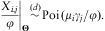
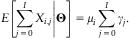
The parameter μi plays the role of the row parameter (related to the exposure of accident year i, see (1.2)), the γj's describe column parameters (related to an incremental claims development (runoff) pattern that is not necessarily normalized, see (1.2)) and ϕ describes the dispersion parameter. We obtain the following first two conditional moments

and the conditional total ultimate claim of accident year i is given by
We analyze the Bayesian ODP Model 1.1 for different types of prior distributions for Θ and different types of parameter estimates for Θ (see (1.3)–(1.4) below).
1.3 Bayesian predictors
Assume the Bayesian ODP Model 1.1 to hold. Using Bayes’ Theorem we find the posterior density of Θ, given the observations  , by
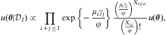
where the proportionality sign ∝ means up to normalization w.r.t. the random vector Θ. In Bayesian theory there are two commonly used predictors, the minimum mean square error (MMSE) predictor and the maximum a posteriori (MAP) predictor for Θ, given  . These are given by


The predictor  minimizes the conditional prediction variance (see also (2.7) below) and the predictor
 is the maximum likelihood estimator (MLE) for the posterior density u(θ|
 ). The MAP predictor
 has the advantage that it can often be calculated analytically. On the contrary, it has a bias term
 , relative to the posterior density u(θ|
 ), that can, in general, only be calculated numerically, for example, using the MCMC methodology. This is discussed in the rest of this paper.
2 Uniform prior distributions and the chain ladder method
In this section we start with uniform priors and log links for the parameters μi and γj. Such a model has already been studied in England & Verrall (Reference England and Verrall2006), Section 7.1. The crucial consequence of the uniform priors assumption is that if we make them non-informative we obtain the classical CL estimate from the MAP predictors. In this spirit, this model is another example that replicates the CL reserves (see also Subsection 2.3).
2.1 The (non-informative) uniform priors model with log link
We define the parameters on the log scale:  and
 .
Model 2.1In addition to Model 1.1 we assume that  are uniformly distributed on (−m, m) for m > 0, and
 are uniformly distributed on (−b, b) for b > 0 and ϕ > 0 is constant.
Remark. It might be more appropriate to use different uniform priors for each parameter, e.g. αi are uniformly distributed on (−mi,mi). However, if we choose non-informative priors for  and
 (i.e. we will let m→∞ and b→∞), then the specific prior differences between the αi's and between the βj's are not relevant.
With (1.1) we obtain

which illustrates the role of the log link function, see also England & Verrall (Reference England and Verrall2002), Section 2.3. That is, with the log link function we derive the generalized linear model form.
The posterior density under Model 2.1 is given by

If we assume that m and b are sufficiently large (we comment on this below) then the MAP predictors for αi and βj can be found by maximizing the posterior log-likelihood function log u(θ| ) analytically, see Section 2.3. This provides MAP estimators
 and
 for αi and βj, respectively, that correspond to the solution of the following system of equations, see also e.g. (2.16)–(2.17) in Wüthrich & Merz (Reference Wüthrich and Merz2008),


Remarks 2.2
•
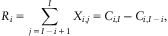
is called the cumulative claim of accident year i up to development year j. The (total) ultimate claim of accident year i is denoted by Ci,I and the outstanding loss liabilities at time I for accident year i are given by(2.3)under the assumption that Xi,j denotes claims payments. The final goal is to predict these outstanding loss liabilities Ri and to determine the prediction uncertainty.• The solution to (2.1)–(2.2) is not unique, i.e. whenever
and solve the system (2.1)–(2.2), then for any also and solve the system (2.1)–(2.2). The requirement m and b sufficiently large now means that there exists at least one such that the solution of (2.1)–(2.2) is within . We fix such a constant K and then denote the resulting MAP predictor by
 is called the cumulative claim of accident year i up to development year j. The (total) ultimate claim of accident year i is denoted by Ci,I and the outstanding loss liabilities at time I for accident year i are given by
 and
 solve the system (2.1)–(2.2), then for any
 also
 and
 solve the system (2.1)–(2.2). The requirement m and b sufficiently large now means that there exists at least one
 such that the solution
 of (2.1)–(2.2) is within
![\[--><$> {{[{\rm{ - }}m,m]}^{I\, + \,1}} \,\times \,{{[{\rm{ - }}b,b]}^{I\, + \,1}} <$><!--](https://static.cambridge.org/binary/version/id/urn:cambridge.org:id:binary:20160319083720764-0452:S1748499512000012_eqnU42.gif?pub-status=live) . We fix such a constant K and then denote the resulting MAP predictor by

The MAP predictor for the outstanding loss liabilities  in (2.3) is then defined by
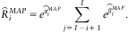
We see that K cancels in this product and hence the specific choice of K is not important as long as at least one such K exists.
• The MAP optimization problem (2.1)–(2.2) can be solved analytically. This is discussed in Section 2.3, below.
• For the priors of αi we can either use informative priors (i.e. m < ∞) or non-informative priors (i.e. m→∞). However, since we have only one parameter, namely m, we always have prior expected value E[αi] = 0 and variance
. Because we would like to have more flexibility in these parameter choices (if we have prior knowledge on αi), we consider different priors in Section 3, which then leads to a Bayesian BF model. For the BF method we refer to Bornhuetter & Ferguson (Reference Bornhuetter and Ferguson1972).• Note that the MAP predictors do not depend on the explicit choices of m, b and ϕ, once m and b are sufficiently large. On the other hand the MMSE predictors will depend on these parameter choices.
 . Because we would like to have more flexibility in these parameter choices (if we have prior knowledge on αi), we consider different priors in
The MMSE predictor for Ri in (2.3) is given by
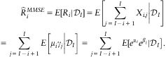
Due to the posterior dependence between αi and βj, given  , this cannot be further decoupled and calculated in closed form, see also Verrall (Reference Verrall2004). Therefore, the MMSE predictor can only be calculated numerically.
We analyze the right-hand side of (2.4) in more detail. We denote  ,
 ,
 ,
 . Doing the following change of variables
 and
 we obtain
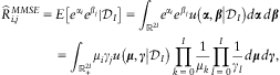
with posterior density
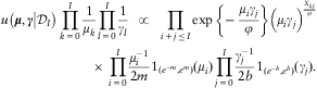
Maximizing the right-hand side of (2.6) provides the MAP estimators  and
 .
Remarks 2.3
• Basically the same remarks about the uniqueness of the MAP estimators
and apply as in Remarks 2.2: (i) they are only unique up to multiplication (and division, respectively) with a positive constant; (ii) we choose m > 0 and b > 0 so large that the mode of the density (2.6) lies within .• The MAP optimization problem (2.6) can be solved analytically. This is discussed in Section 3.2, below.
• The MAP predictor for the outstanding loss liabilities Ri in (2.3) is then defined by
 and
 apply as in Remarks 2.2: (i) they are only unique up to multiplication (and division, respectively) with a positive constant; (ii) we choose m > 0 and b > 0 so large that the mode of the density (2.6) lies within
![\[--><$> {{[{{e}^{{\rm{ - }}m}} \,,\,{{e}^m} ]}^{I\, + \,1}} \,\times \,{{[{{e}^{{\rm{ - }}b}} \,,\,{{e}^b} ]}^{I\, + \,1}} <$><!--](https://static.cambridge.org/binary/version/id/urn:cambridge.org:id:binary:20160319083720764-0452:S1748499512000012_eqnU61.gif?pub-status=live) .
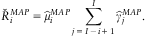
This now leads to a slightly unpleasant observation. Note that the MMSE predictor in (2.5) does not depend on the parametrization. This is not true for the MAP predictor! The MAP estimators  and
 solve the system of equations (2.1)–(2.2), whereas the MAP estimators
 and
 will solve the system of equations (3.11)–(3.12), below. Because these two systems of equations differ, we find

This property is well known in Bayesian statistics, see for example Smith (Reference Smith1998). It gives us a first indication that the MAP predictor is not always suitable in a Bayesian context.
2.2 Prediction uncertainty
We measure the prediction uncertainty in terms of the conditional mean square error of prediction (MSEP) which for a  -measurable predictor
 for Ri is given by, see also Section 3.1 in Wüthrich & Merz (Reference Wüthrich and Merz2008),

From (2.7) we see that the MMSE predictor ![\[--><$> \widehat{R}_{i}^{{MMSE}} \, = \,E\left[ {{{R}_i}|{{\cal D}_I}} \right] <$><!--](https://static.cambridge.org/binary/version/id/urn:cambridge.org:id:binary:20160319083720764-0452:S1748499512000012_eqnU71.gif?pub-status=live) minimizes the conditional MSEP. The conditional MSEP for the MAP predictor is given by

The MMSE predictor and the conditional MSEP can, in general, only be determined numerically, using e.g. the MCMC methodology.
First conclusions. In many situations the MAP predictor  has the advantage over the MMSE predictor
 that it can be calculated analytically. The MMSE predictor on the other hand has the advantage that it minimizes the prediction uncertainty if we use the conditional MSEP as uncertainty measure. The MAP predictor obtains a positive bias term
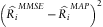 , see (2.8). This bias term however needs to be interpreted carefully: it is always measured w.r.t. the posterior density u(θ|
 .
2.3 Link to the chain ladder algorithm
The remarkable property of the MAP predictor  in Model 2.1 with non-informative priors and log link is that it is equal to the CL reserves
 . That is, the non-informative priors Bayesian Model 2.1 with MAP predictors is another stochastic model that leads to the CL reserves: since our system (2.1)–(2.2) of equations is exactly the same as the one for the ODP model, see (2.16)–(2.17) in Wüthrich & Merz (Reference Wüthrich and Merz2008), we have

In the literature this was, for example, proved by Mack (Reference Mack1991). Therefore, we define for j = 0,…,I – 1 the CL factor estimators

Corollary 2.18 and Remarks 2.19 in Wüthrich & Merz (Reference Wüthrich and Merz2008) then imply that (for the appropriate normalizing constant K)
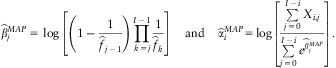
That is, we can explicitly calculate the MAP predictors. Moreover, this gives another stochastic model that allows for the calculation of the conditional MSEP given in (2.8). Unlike in Mack's (1993) distribution-free CL model and in the ODP model (see England & Verrall (Reference England and Verrall2002), Section 7.2) we do not need any approximations here for the estimation of the MSEP, but we calculate the exact conditional MSEP value (2.8) numerically in this Bayesian inference model (using the MCMC methodology).
In this spirit the parameter uncertainty of the estimate Θ is part of the model, see (2.8). Moreover, because we have all key figures in terms of the full posterior distributions, we can calculate any risk measure of interest (not only the conditional MSEP).
3 Gamma prior distributions
In Section 2 we have used uniform priors with log links in order to obtain the CL reserves. In this section gamma prior distributions (with the identity link) are used, especially for the modelling of the row parameters μi. This allows us to incorporate prior expert knowledge about the model parameters and we obtain claims reserves in a similar spirit to the BF method. However, in our model, we still have the freedom to determine how much credibility weight we give to the prior knowledge. A similar Bayesian ODP model with gamma priors has, for example, already been studied in Section 7.11 of England & Verrall (Reference England and Verrall2002) and Example 4.51 of Wüthrich & Merz (Reference Wüthrich and Merz2008).
3.1 Informative priors for the row parameters
Model 3.1In addition to Model 1.1 we assume that μi are Γ-distributed with mean mi > 0 and shape parameter ai > 0, γj are Γ-distributed with mean cj > 0 and shape parameter b > 0, and ϕ > 0 is constant.
In contrast to Model 2.1, we now extend the prior model for μi to a two-parameter distribution. Our aim is to keep the mean mi fixed and study the sensitivity in the shape parameter ai. The priors for γj will be chosen to be non-informative (i.e. b→0).
The posterior density (likelihood function) in Model 3.1 is given by

The MAP predictors using non-informative priors for γj (i.e. b→0) are then found by solving


with adjusted incremental claims

and adjusted cumulative claims  .
Therefore, the MAP predictors for non-informative claims development pattern γj will be a function of the parameters ϕ, m = (m 0,…,mI) and a = (a 0,…,aI).
Lemma 3.2 We assume Model 3.1 is fulfilled, and we assume that  for all i = 0,…,I and
 for all j = 0,…,I. The solution to (3.2)–(3.3)satisfies μi > 0 and γj > 0 for all ai ≥ 0 and i,j = 0,…,I.
We first state a CL type result. Note that in the following lemma we do a CL argument on the rows instead of on the columns; and for a = 0 we obtain the CL method on rows. Its proof is similar to the classical CL result, see e.g. Section 2.4 in Wüthrich & Merz (Reference Wüthrich and Merz2008).
Lemma 3.3 In Model 3.1 equations (3.2)–(3.3) imply for j = 0,…,I−1
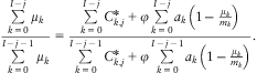
The statement of Lemma 3.3 can also be written in incremental form, i.e. for i = 1,…,I
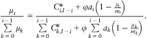
This implies the following theorem:
Theorem 3.4 In Model 3.1 equations (3.2)–(3.3) imply for i = 1,…,I

and

Theorem 3.4 is now the key to obtain the MLE which are the same as the solutions of equations (3.2)–(3.3). Note that the right-hand side of (3.5) only depends on μ 0,…,μi −1. Therefore, once we know the initial value  , the remaining estimators for μ 1,…,μI are calculated iteratively by (3.5). This is discussed in more detail below.
Solution to (3.2)–(3.3)fora∈(0,∞). We apply Theorem 3.4. Choose an initial value  , then using (3.5) we define iteratively for i = 1,…,I

where we have defined
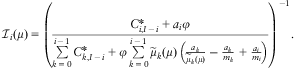
Note that the vector  is now a function of one single parameter μ > 0. The MAP predictors for (3.2)–(3.3) are then found by using the normalizing condition (3.6), that is, choose μ > 0 such that

We denote the resulting MAP predictors for 0 ≤ I, j ≤ I by

where  is obtained from (3.3).
• Predictors in the gamma priors Model 3.1 are denoted by a superscript “*”, e.g.
, whereas predictors in the uniform priors Model 2.1 are simply denoted by and , respectively, depending on the parametrization (2.5).• Note that the MAP predictors can now easily be found by a simple (one-dimensional) root searching algorithm (it only depends on one single parameter μ > 0, see (3.7)). This is slightly more involved than the closed form solution (2.10) in the uniform prior case, but it is a lot simpler than the multi-dimensional generalized linear model (GLM) claims reserving problems where one either uses the Newton-Raphson algorithm or Fisher's scoring method to find the roots for the multidimensional problems, see for example Chapter 6 in Wüthrich & Merz (Reference Wüthrich and Merz2008).
• For the special case of
and we obtain a closed form solution. Equation (3.5) implies for constant mi and ai
 , whereas predictors in the uniform priors Model 2.1 are simply denoted by
 and
 , respectively, depending on the parametrization
 and
 we obtain a closed form solution. Equation
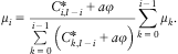
The normalization condition (3.6) then provides
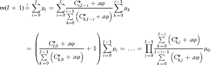
Hence, from this we can explicitly calculate the MAP predictor
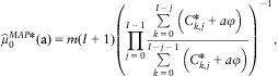
and the iteration then provides the remaining MAP predictors.
• We can now study the MAP predictors as a function of the degree of information a contained in the prior estimates mi, in particular, we obtain a smoothed claims development pattern
, where the degree of smoothing depends on a.
 , where the degree of smoothing depends on a.
The MAP predictor for the outstanding loss liabilities of accident year i > 0 is then given by

3.2 Non-informative prior case
For the non-informative prior case we let ai→0 for all i. The posterior density (likelihood function) in Model 3.1 for non-informative priors is then asymptotically given by

There are two important observations: (i) The non-informative prior case in Model 3.1 has exactly the same posterior density as the non-informative prior case in Model 2.1 “under the change of variables’’, see (3.10) and (2.6) for m,b→∞. Therefore, the predictive posterior distributions of the outstanding loss liabilities Ri in these two non-informative priors models will coincide as well as their MAP predictors. (ii) Note that in the case (3.10) the last terms on the left-hand side and the right-hand side of (3.2) disappear. Therefore, we are left with


Similar to the solution of (2.1)–(2.2) we find the following solutions to (3.11)–(3.12)

for any positive constant e K and CL factors  for the transformed observations


Therefore, we obtain a CL model for the incremental claims  . However, in this case we can find a “natural’’ normalizing constant e K. Theorem 3.4 implies
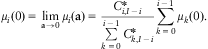
Proposition 3.6 In Model 3.1 equations (3.2)–(3.3)imply

Therefore, Proposition 3.6 provides a natural scaling constant  if we let the degree of information a converge to 0.
3.3 Strong prior case
For the strong prior case we let ai→∞ for all i and obtain from (3.2)–(3.3)


Therefore,  and

In this case we can explicitly calculate the posterior distributions of γj, given  . These posterior distributions are independent with

This immediately implies that
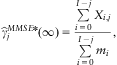
and the bias of the MAP predictor of γj is given by
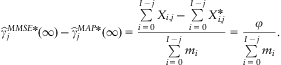
Therefore, in the strong prior case we obtain closed form posterior distributions which allow for an analytical analysis of the model, both for the MAP predictor

and the MMSE predictor

3.4 Link to the Bornhuetter & Ferguson (Reference Bornhuetter and Ferguson1972) method
The BF method, as applied in practice, uses as claims development pattern γj the one implied by the CL factor estimates given in (2.10). Therefore, the classical BF predictor for the outstanding loss liabilities is given by
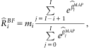
where the  's solve (2.1)–(2.2).
 exactly corresponds to the BF predictor studied in Alai et al. (Reference Alai, Merz and Wüthrich2009).
Mack (Reference Mack2008) provides a different BF predictor where he uses a different method for the estimation of the claims development pattern γj. We include a comparison of the results with two versions of the Mack (Reference Mack2008) method. In the first case we define the raw pattern, see formula (3) in Mack (Reference Mack2008),
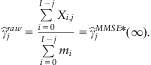
This pattern is not normalized, i.e. does not add up to 1. Therefore, we can also study a second development pattern defined by

We then define similar to Mack (Reference Mack2008)

These BF predictors  ,
 and
 can now be compared to the CL predictor
 as well as to the MAP predictors
 , for ai∈[0,∞] and the corresponding MMSE predictors. In this spirit, the Bayesian predictors can be viewed as BF predictors where ai determines the degree of information contained in the prior value mi. These predictions and estimators are compared in Section 5.
Moreover,  and
 can be viewed as smoothed claims development patterns where we account for the prior information mi according to its degree of information ai for smoothing.
4 Bias, prediction uncertainty and MCMC
4.1 Gibbs sampler
In general, Models 2.1 and 3.1 do not allow for analytical calculations of the posterior distributions. In most cases the posterior distribution of the parameters can only be determined up to the normalizing constant. This is then the ideal situation to apply MCMC simulation methods which provide empirical posterior distributions. These empirical posterior distributions then allow for the calculation of claims reserves, cash flows and any desirable risk measure. For an introduction to MCMC methods we refer to Gilks et al. (Reference Gilks, Richardson and Spiegelhalter1996), Asmussen & Glynn (Reference Asmussen and Glynn2007) and Spiegelhalter et al. (Reference Spiegelhalter, Thomas, Best and Gilks1995, Reference Spiegelhalter, Best, Carlin and van der Linde2002). We mention that in recent actuarial literature MCMC methods became rather popular, see e.g. Scollnik (Reference Scollnik2001) and the literature therein, England & Verrall (Reference England and Verrall2002, Reference England and Verrall2006) and Section 4.4 in Wüthrich & Merz (Reference Wüthrich and Merz2008).
Here, we use the Gibbs sampler, see Gilks et al. (Reference Gilks, Richardson and Spiegelhalter1996), page 12. The Gibbs sampler is a simplified version of the single-component Metropolis-Hastings algorithm (Metropolis et al., Reference Metropolis, Rosenbluth, Rosenbluth, Teller and Teller1953, Hastings, Reference Hastings1970). Our aim is to sample from the posterior density u(θ| ) with
 , see (3.1). This posterior density has the special property that


Thus, from these conditional posterior densities u (μ| ) and u (
 ,μ) we can directly sample from. The Gibbs sampler then goes as follows:
1. Initialize
.2. For t ≥ 1 do
(a) generate
(b) generate
(c) set
.
 .


 .
Then, this algorithm provides a Markov chain  whose stationary limit distribution is given by u(θ|

 ), see Gilks et al. (Reference Gilks, Richardson and Spiegelhalter1996) and Asmussen & Glynn (Reference Asmussen and Glynn2007).
4.2 Empirical distribution from Gibbs sampling
Using the Gibbs sampler we obtain (after burn-in T) an empirical distribution from the sample

which is an estimator for the posterior distribution u(·| ). Therefore, we estimate the MMSE predictor
 by the sample mean

To indicate that this is the sample mean we use two hats in the notation. The conditional MSEP of the MMSE predictor is estimated similarly. Note that
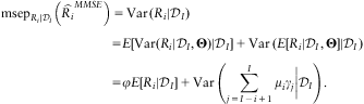
Therefore, we get the estimator

Remarks 4.1
• We would like to emphasize that using the Gibbs sampler we do not only estimate the conditional MSEP. The Gibbs sampler provides an approximation to the full posterior distribution u(·|
) and one can calculate any desirable risk measure.• The empirical sample
allows for the simulation of the payments Xi,j: for any t > T we may sample for i + j > I
 ) and one can calculate any desirable risk measure.
 allows for the simulation of the payments Xi,j: for any t > T we may sample for i + j > I

This provides the simulated cash flows. The sampled outstanding loss liabilities Ri are then obtained by
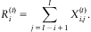
The sample  then provides the empirical posterior distribution of Ri, given
 , see also Figure 2. Moreover, it also allows for the direct estimation of (4.1), simply by calculating the sample variance of the simulated values.
5 Example
5.1 Univariate example
Before we start with a real data example (in the next subsection) we illustrate the behaviour of the MAP and the MMSE predictors in a univariate example. This example highlights the importance of the choice of the prior distribution, the link function and its implications.
Assume conditionally, given Λ, X 1,…,Xn, Xn +1 are i.i.d. Poisson distributed with parameter Λ. We assume that X 1,…,Xn are observed and we would like to make Bayesian inference for Λ and Xn +1.
We now make different choices for the distribution Λ:
Case 1. Γ = log(Λ) has a non-informative uniform prior distribution. In that case the posterior distribution of Γ, given X = (X 1,…,Xn), is given by
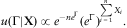
This implies

In this case the MAP and the MMSE predictors coincide.
Case 2. We make the same assumptions as in Case 1 but we do a change of variable in (5.1). We set Λ = e Γ this provides posterior density
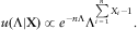
This implies

That is, we obtain  . This shows that the MAP predictors are not invariant under re-parametrization and therefore are often not appropriate. This is well-known in Bayesian theory, see for example Smith (Reference Smith1998).
Case 3. Λ has a non-informative gamma prior distribution. In that case the posterior distribution of Λ, given X, has exactly the same form as in Case 2 and therefore we obtain the same inference picture as in Case 2.
Case 4. Λ has the non-informative Jeffrey's prior distribution  . In that case the posterior distribution of Λ, given X = (X 1,…,Xn), is given by
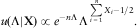
Jeffrey's non-informative priors are often used because they have invariance properties under parameter transformations. This implies

In this paper we do not further investigate Jeffrey's priors.
Conclusion. The MMSE predictor  has always minimal posterior variance and is invariant under re-parametrization. Therefore the optimal Bayesian predictor for Xn +1, given
 , is always given by

5.2 Real data example
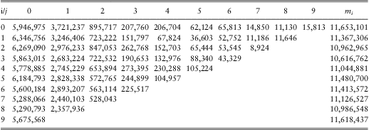
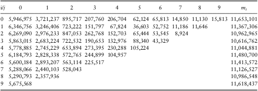
We revisit the BF example given in Tables 2.2–2.4 of Wüthrich & Merz (Reference Wüthrich and Merz2008) (this is the example also considered in the BF analysis in Alai et al., Reference Alai, Merz and Wüthrich2009)), see Table 1. We analyze this data set for non-informative uniform priors according to Model 2.1 and for gamma priors according to Model 3.1. In order to compare the results to the results in Wüthrich & Merz (Reference Wüthrich and Merz2008) and Alai et al. (Reference Alai, Merz and Wüthrich2009) we choose a fixed plug-in estimate ϕ = 14,714.
Observed incremental claims Xi,j, i + j ≤ I, and prior values mi.
5.2.1 Non-informative priors and the CL method
In this subsection we study Model 2.1 with non-informative uniform priors and log link as well as Model 3.1 with non-informative gamma priors. The Gibbs sampler allows us to numerically calculate the MMSE predictors

for Model 2.1 (with m,b→∞) and Model 3.1 (with  and b→0). In Model 2.1 the posterior density is then given by (2.5)–(2.6) with m,b→∞. In Model 3.1 the posterior density is then given by (3.10).
Note that for these two non-informative prior cases the posterior densities coincide, see (2.6) and (3.10). Therefore, we only need to run one Gibbs simulation to solve both of these two cases numerically.
We have used the Gibbs sampler and we have run 1,000,000 simulations after the subtraction of burn-in costs T = 100,000. This provided the empirical posterior distribution of the parameters  from which the MMSE predictors and their empirical uncertainty
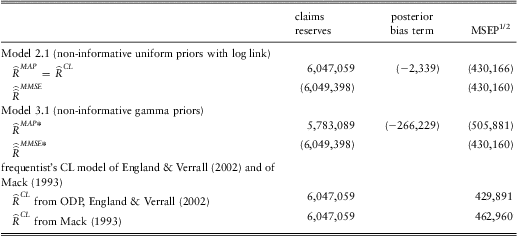
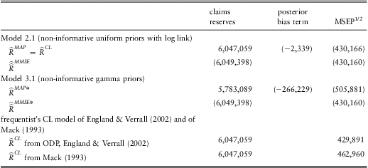
 were provided, see Section 4.2. For the estimation of the prediction uncertainty of the MAP predictor we have used formula (2.8). The results are presented in Table 2.
Claims reserves predictors with corresponding conditional MSEP1/2 in Model 2.1 (with non-informative uniform priors and log link) and in Model 3.1 (with non-informative gamma priors). The figures in brackets are obtained by Gibbs sampling, the others are exact. The results are compared to the frequentist's CL model of England & Verrall (Reference England and Verrall2002) and of Mack (Reference Mack1993). Note that Mack (Reference Mack1993) is a rather different model, so we include Mack's (Reference Mack1993) results only for comparison purposes.
Observations 5.1
• We observe that the predictors of the outstanding loss liabilities are all rather similar in these non-informative prior situations. The MAP predictor
coincides with the CL reserves and it is also in line with the MMSE predictors obtained by Gibbs sampling. Only the MAP predictor in the non-informative gamma priors Model 3.1 gives a prediction that deviates from the others. This prediction seems too low and moreover, as mentioned in Remarks 2.3, the MAP predictor is not invariant under re-parametrization. Therefore its use is questionable.• Note that although the MAP predictors for Models 2.1 and 3.1 (with non-informative priors) are different, the distributions of the reserves are identical since they are from the same Gibbs simulation. This highlights the danger of focusing solely on the MAP predictors, and not on the distribution.
• Prediction uncertainties in terms of the conditional MSEP: We compare our Bayesian calculations to the frequentist's estimates found in the literature: (i) ODP (constant scale) analytical approximation using asymptotic normality of MLEs, see Section 7.2 in England & Verrall (Reference England and Verrall2002), (ii) distribution-free CL method, see Mack (Reference Mack1993):
We observe that our Bayesian models provide a prediction uncertainty in the range of 430,000. This is very similar to the estimate of England & Verrall (Reference England and Verrall2002) in the asymptotic normality approximation. Mack (Reference Mack1993)'s model is a rather different model, therefore we include Mack's (Reference Mack1993) results only for comparison purposes.• The Bayesian models now have the advantage that they provide the full posterior parameter distributions. Therefore, we can calculate the predictive distribution of the outstanding loss liabilities (not only the claims reserves and the conditional MSEP). This is further outlined below.
 coincides with the CL reserves
 and it is also in line with the MMSE predictors
 obtained by Gibbs sampling. Only the MAP predictor in the non-informative gamma priors Model 3.1 gives a prediction
 that deviates from the others. This prediction seems too low and moreover, as mentioned in Remarks 2.3, the MAP predictor is not invariant under re-parametrization. Therefore its use is questionable.

5.2.2 Informative gamma priors
We turn to Model 3.1 (gamma priors) with informative priors, that is, we implement prior knowledge about the exposure parameters μi. We choose the degree of information a constant for all accident years, i.e. ![\[--><$> {{a}_i}\, \equiv \,a\, \in \,[0,\infty ] <$><!--](https://static.cambridge.org/binary/version/id/urn:cambridge.org:id:binary:20160319083720764-0452:S1748499512000012_eqnU188.gif?pub-status=live) . Then the MAP predictors in Model 3.1 are given by

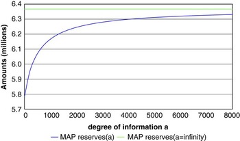
These are calculated by the root searching algorithm given in (3.7) for a∈(0,∞), the cases a = 0 and a = ∞ can be solved explicitly. Figure 1 gives the MAP predictors  for different degrees of information a∈[0,∞]. We see that in our case the claims reserves
 are an increasing function in the degree of information a. This comes from the fact that the prior estimates mi are rather conservative (this will be further highlighted below).
MAP predictors  for different degrees of information
![\[--><$> a \in [0,\infty ] <$><!--](https://static.cambridge.org/binary/version/id/urn:cambridge.org:id:binary:20160319083720764-0452:S1748499512000012_eqnU248.gif?pub-status=live) .

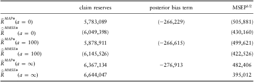
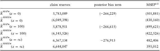
Next, we determine the MMSE predictors and the prediction uncertainties in the gamma priors model. Therefore we again apply the Gibbs sampler. After subtracting the burn-in costs T = 100,000 we again simulate 1,000,000 samples. The results are provided in Table 3.
Claims reserves predictors with corresponding conditional MSEP1/2 in the gamma Model 3.1 for different degrees of information a. The figures in brackets are obtained by Gibbs sampling.
Observations 5.2
• The first observation is that in the Gibbs sampler we obtain long-range dependencies for later development periods. This comes from the fact that we have large variances (for non-informative priors) and only a few observations. Therefore, we need many simulations (
large) for the convergence of the empirical mean.• Similar to the non-informative gamma prior case we see substantial posterior bias terms in the MAP predictors. This comes from the fact that the dispersion ϕ is fairly large compared to the incremental payments Xi,j in later development periods. For a = ∞, for example, this results in
which explains the posterior bias terms. This again indicates that the MAP predictors should not be used.• We see that the MMSE predictors are increasing in the degree of information a. This comes from the fact that the prior means mi were chosen rather conservative and the more weight we give to these conservative prior means the more the MMSE predictors increase.
• The conditional MSEPs are decreasing in the degree of information a. This is rather obvious because the less uncertainty we have in the prior distributions the less prediction uncertainty we obtain. We see that the conditional
decreases from 430,160 to 395,012.
 large) for the convergence of the empirical mean.
 which explains the posterior bias terms. This again indicates that the MAP predictors should not be used.
 decreases from 430,160 to 395,012.
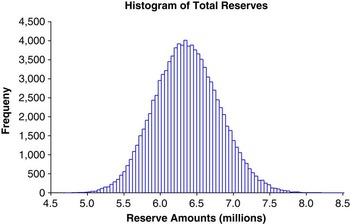
As mentioned above, we obtain the full posterior distribution from the Gibbs sampler for the outstanding loss liabilities  , conditional on
 , see (4.3). We consider in Model 3.1 the case a = 100. The histogram of the total reserves from 100,000 simulation of the outstanding loss liabilities R is given in Figure 2.
Histogram for  in Model 3.1 for a = 100 from 100,000 simulations.

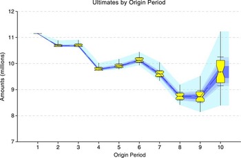
This empirical distribution now allows for the estimation of any risk measure, not only the conditional MSEP. Moreover, we can also plot confidence intervals, for example, in Figure 3 we show the confidence intervals per accident year i. As expected, we observe that the uncertainty in old accident years is rather low, because they are already well developed, whereas for younger accident years we obtain bigger ranges.
Confidence intervals of  , i = 1,…,10, in Model 3.1 for a = 100. The different quantiles correspond to: minimum, 5th percentile, 10th percentile, 25th percentile, 50th percentile, 75th percentile, 90th percentile, 95th percentile and maximum.

The Gibbs sampler not only provides the conditional distribution of the outstanding loss liabilities Ri, given  , but we also obtain the conditional distribution of the cash flows Xi,j, conditionally given
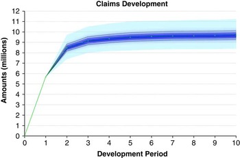
 . From these cash flows we can determine how the uncertainty evolves over time (over the development years). In Figure 4 we show the development of the uncertainty over time for the youngest accident year. We see that the payment for the first development year is given (contained in
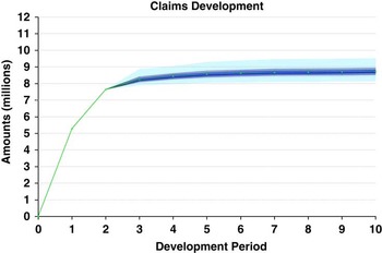
 ). This is why there is no uncertainty at time 1. After this first development year we obtain the corresponding confidence intervals. Figure 5 describes the same development uncertainty but for the second youngest accident year. Of course, we observe a smaller uncertainty, because we have more observations compared to the case in Figure 4.
Development of Ci,j, i = I and j ≥0, over time in Model 3.1 for a = 100. The different gray scales correspond to: 10th percentile, 25th percentile, 50th percentile, 75th percentile, 90th percentile.

Development of Ci,j, i = I–1 and j ≥0, over time in Model 3.1 for a = 100. The different gray scales correspond to: 10th percentile, 25th percentile, 50th percentile, 75th percentile, 90th percentile.

5.2.3 Strong gamma prior case and the BF method
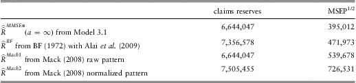
Finally, we compare the gamma priors Model 3.1 with strong priors for μi to the classical BF predictor. In the literature the classical BF predictor is given by (3.16). We also compare the classical BF predictor to the BF predictors obtained from Mack (Reference Mack2008):


For the calculation of the prediction uncertainty of the BF predictor there are different methods in the literature: The conditional MSEP  of the classical BF predictor is calculated with Alai et al. (Reference Alai, Merz and Wüthrich2009) and the conditional MSEPs
 and
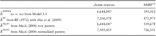
 of the BF-Mack predictors are calculated according to Mack (Reference Mack2008). The results are presented in Table 4.
Claims reserves predictors with corresponding conditional MSEP1/2 according to Model 3.1 with strong priors, Alai et al. (Reference Alai, Merz and Wüthrich2009) and Mack (2008).
Observations 5.3
• The different BF predictors are rather diverse. This comes from the fact that the prior values mi are too high, which has the rather unpleasant effect that we do not obtain reliable estimates for the claims development pattern γj. For the raw pattern we obtain
. If we normalize this raw pattern, we get predictors and that are too high. Also the non-normalized ones and seem to be too high because of the large values of mi.• The predictors
and coincide because they use the same parameter estimates. However, the underlying reasoning is slightly different which can be seen in the prediction uncertainty. For the MMSE predictor there is no uncertainty in mi (because we assume perfect information a = ∞), whereas in we also add uncertainty to mi.• The gamma priors Model 3.1 is consistent in the sense that it also uses the prior knowledge on μi to estimate the claims development pattern γj (whereas the other BF methods are not). In this spirit our Bayes model should be preferred. Moreover, we also have the flexibility to attach credibility weights in terms of a to this prior knowledge which then results in Table 3.
 . If we normalize this raw pattern, we get predictors
 and
 that are too high. Also the non-normalized ones
 and
 seem to be too high because of the large values of mi.
 and
 coincide because they use the same parameter estimates. However, the underlying reasoning is slightly different which can be seen in the prediction uncertainty. For the MMSE predictor
 there is no uncertainty in mi (because we assume perfect information a = ∞), whereas in
 we also add uncertainty to mi.
6 Conclusions
The Bayesian ODP claims reserving model with uniform priors and log link (Model 2.1) and with gamma priors (Model 3.1) give mathematically consistent ways to estimate claims reserves in the Bornhuetter & Ferguson (Reference Bornhuetter and Ferguson1972) spirit:
• they use prior knowledge mi for the expected ultimate claim;
• they combine the prior knowledge mi with an estimated claims development pattern
to obtain the reserves;• this claims development pattern is estimated using a credibility weighted average between the observations
and the prior knowledge mi according to the degree of information a contained in the prior knowledge. Complete prior knowledge (a = ∞) leads to a BF model similar to Mack (Reference Mack2008), no prior knowledge (a = 0) leads to the CL case, and for a∈(0,∞) we can model any intermediate case.
 to obtain the reserves;
 and the prior knowledge mi according to the degree of information a contained in the prior knowledge. Complete prior knowledge (a = ∞) leads to a BF model similar to Mack (
The advantage of such full Bayesian models is that they allow for a complete analysis and for the calculation of any risk measure, whereas the frequentist's approaches (Alai et al. (Reference Alai, Merz and Wüthrich2009) and Mack (Reference Mack2008)) need additional approximations for the determination of the conditional MSEP, and are unable to provide additional information such as predictive distributions of cash flows.
Limitations and outlook for further research. This paper only considers the ODP model with constant scale factor ϕ, and the BF model in the context of the CL model without a tail factor. In many cases the choice of a constant scale parameter ϕ should be checked. Often data suggests that ϕ j depends on the development period j. Furthermore, it should be checked whether the conditional independence assumption between the Xi,j's is appropriate and whether one should include tail factors beyond the latest development period.
A Proofs
Proof of Lemma 3.2. This is an immediate consequence of the assumptions and (3.2)–(3.3).□
Lemma A.1In Model 3.1 equations (3.2)–(3.3) imply for j = 0,…,I

Proof of Lemma A.1. We first prove the two statements (an empty sum is set equal to 0)


If we sum (3.2) over i = 0.…,I and (3.3) over j = 0.…,I we obtain

This immediately implies statement (A.2). We now turn to (A.1). The proof is similar to the proof of Lemma 2.17 in Wüthrich & Merz (Reference Wüthrich and Merz2008) and goes by induction.
We start with j = 0: using (3.3) in the second step we have
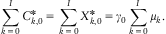
This proves the claim for j = 0.
Induction step j→j + 1. We assume that the claim holds true for j ≤ I−1, then we prove the claim for j + 1:

To the first term on the right-hand side we apply the induction assumption

and to the second and third term (3.2) and (3.3), respectively. This implies
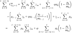
This proves (A.1). If we now combine (A.1) and (A.2) we obtain

This proves the claim.□
Proof of Lemma 3.3. Choose j ≤ I–1 then we have from Lemma A.1 and equation (3.2)
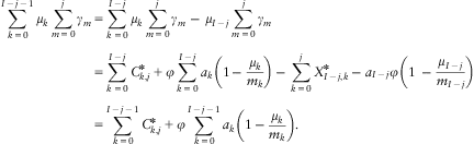
If we divide the equality in Lemma A.1 by (A.3) we obtain the claim.□
Proof of Theorem 3.4. We solve (3.4) for μi. In a first step we obtain for i = 1,…,I

Moreover, we have

Therefore, if we divide by the bracket on the left-hand side we obtain
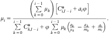
But then the first claim easily follows. The second claim was already proved in (A.2).□
Proof of Proposition 3.6. The proof follows from the normalization condition (3.6) and (3.13) similar to the derivation (3.8).□