Introduction
The full-field electroretinogram (ERG) is a measure of the mass electrical response of the retina to light stimulation. The human ERG is typically recorded in response to stimuli with various luminances, wavelengths, and temporal properties, and under different adaptation conditions, in order to evaluate the functional integrity of the retina (Marmor et al., Reference Marmor, Fulton, Holder, Miyake, Brigell and Bach2009). In particular, the ERG response to a stimulus flickering at approximately 30 Hz is recorded under light-adapted conditions in the clinical setting to assess the function of the cone system in patients with retinal diseases. The standard measures of the flicker ERG response are the peak-to-trough amplitude and the implicit time (time-to-peak). However, there are other features of the flicker ERG that are not routinely examined but that may provide useful information about retinal function.
One such feature of the human cone flicker ERG is the presence of additional responses that are observed at certain stimulus frequencies following the termination of a flicker train. The first of these additional responses is present at stimulus frequencies above 38 Hz, and its characteristics have been described previously (McAnany & Alexander, Reference McAnany and Alexander2009). Between stimulus frequencies of 38 and 63 Hz, this first additional response is characterized by a constant delay between its peak and the peak of the stimulus cycle that would have followed the last actual stimulus cycle if the flicker train had continued. That is, the first additional ERG response following the termination of a flicker train appears to be generated by a stimulus cycle that is not physically present.
This first additional poststimulus response is of particular interest due to the similarity in its timing properties to a phenomenon that has been reported to occur in retinal ganglion cell (RGC) recordings from salamander and mouse (Schwartz et al., Reference Schwartz, Harris, Shrom and Berry2007; Schwartz & Berry, Reference Schwartz and Berry2008). In these RGC recordings, the interruption or termination of a train of repetitive stimuli can elicit an additional response whose timing is constant with respect to the stimulus cycle that is omitted from the train. The additional RGC response has been termed an “omitted stimulus response” (OSR) because it appears to be generated by a stimulus that is not physically present, termed an “omitted stimulus” (OS) (Schwartz et al., Reference Schwartz, Harris, Shrom and Berry2007; Schwartz & Berry, Reference Schwartz and Berry2008).
In addition to the first additional OSR-like response reported previously in the human cone flicker ERG (McAnany & Alexander, Reference McAnany and Alexander2009), multiple additional ERG responses can also be observed following the termination of a flicker train. The origin of these multiple additional responses is uncertain. One possibility is that they represent a continuing response to the terminated flicker train. If that is the case, then the period of the additional poststimulus responses would correspond to the period of the flicker train. A second possibility is that the additional poststimulus responses are generated by a resonant mechanism. A resonant system, specifically an LRC electrical circuit involving inductance (L), resistance (R), and conductance (C), has been used to model resonances in ON bipolar cells of the salamander retina (Gao et al., Reference Gao, Schwartz, Berry and Holmes2009). If a similar type of resonant mechanism underlies the generation of the multiple poststimulus responses of the human cone flicker ERG, then the period of the additional responses would not necessarily correspond to the period of the stimulus flicker train.
The purpose of this study was to evaluate these two possibilities by examining the temporal properties and amplitude characteristics of the multiple poststimulus responses observed in the human cone flicker ERG. Additionally, we evaluated whether the properties of the multiple poststimulus responses are described adequately by a mathematical model of a resonant system.
Methods
Subjects
The ERG recordings that were analyzed in this study were obtained from 10 visually normal subjects (7 female and 3 male, ages 23 to 55 years). These waveforms were also the basis for a previous study of the flicker ERG (McAnany & Alexander, Reference McAnany and Alexander2009). All subjects had best-corrected visual acuity of 20/20 or better in the tested eye as measured with a Lighthouse Distance Visual Acuity Chart, normal letter contrast sensitivity as measured with a Pelli–Robson Contrast Sensitivity Chart, clear ocular media, and a normal-appearing fundus on ophthalmic examination. The study was approved by an institutional review board at the University of Illinois at Chicago, and informed consent was obtained from each subject prior to data collection in accordance with principles embodied in the Declaration of Helsinki.
Stimuli and recording system
The stimuli and recording system have been described in detail previously (McAnany & Alexander, Reference McAnany and Alexander2009). In brief, the test stimuli consisted of sinusoidally modulated full-field flicker that was composed of equal luminances of middle-wavelength (512-nm peak) and long-wavelength (632-nm peak) light, generated by arrays of light-emitting diodes (LEDs) housed within a Diagnosys ColorDome desktop Ganzfeld (Diagnosys LLC, Littleton, MA). The yellow-appearing flicker, which had a mean luminance of 200 cd/m2 (4.0 log td, assuming a dilated pupil diameter of 8 mm) and a nominal Michelson contrast of 100%, was presented against a steady, rod-saturating, short-wavelength adapting field (468-nm peak) that had a luminance of 12.3 cd/m2 (2.8 log td, equivalent to 3.3 log scot td). During the intervals between the flicker presentations, the ColorDome Ganzfeld was illuminated with a steady uniform field with the same spectral characteristics and mean luminance as during the flicker presentations. Stimulus luminances and spectral characteristics were measured with a PR-650 Spectra-Scan colorimeter (Photo Research, Inc., Chatsworth, CA). Photopic luminances were based on V10(λ).
ERG potentials were recorded using a Burian–Allen bipolar electrode wetted with methylcellulose. A ground electrode was attached to the ipsilateral earlobe. Signals were acquired with a Diagnosys Espion electrophysiology console, using amplifier band-pass settings of 0.3 to 500 Hz (without a 60-Hz notch filter) and a sampling frequency of 2 kHz.
Procedure
Prior to an ERG recording, the pupil of the tested eye was dilated using 2.5% phenylephrine and 1% tropicamide drops and the cornea was anesthetized with proparacaine drops while the subject was exposed to room illumination. The electrode insertion was done under room illumination, and then the subject adapted to the stimulus mean luminance for 5 min, which was sufficient to achieve a state of constant light adaptation. Only one eye of each subject was tested, and the nontested eye was occluded using an eye patch.
ERG responses were recorded to flicker trains ranging in frequency from 6.3 to 100 Hz, presented in order of increasing frequency, but only the responses at frequencies from 31.25 to 100 Hz were analyzed for this study. Each stimulus was presented for approximately 1 s. The exact duration of presentation depended on the stimulus period. Each recording was synchronized with the onset of the flicker presentation and the recording continued for an additional six stimulus periods following flicker train offset. At each frequency, ERG responses were recorded to at least three stimulus presentations, with the number of repetitions depending on ERG response quality. The analyses were based on the means of the three responses with the least noise and eye movement artifacts.
Results
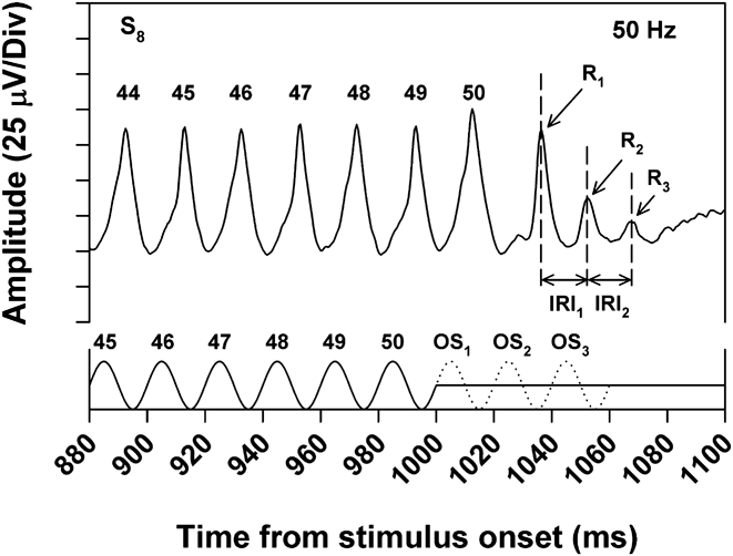
Fig. 1 illustrates the mean ERG response of a typical subject toward the end of a 50-Hz flicker train. The solid trace along the x-axis represents the stimulus waveform. There were 50 stimulus cycles in the flicker train, indicated by the numbers above the stimulus peaks. Following the final stimulus cycle, the luminance returned to the mean level. The dotted trace represents the first three “omitted stimuli” (OS1, OS2, and OS3, referring to the next three stimulus cycles that would have occurred if the flicker train had continued). The numbers above the ERG peaks indicate the responses to the correspondingly numbered stimulus peaks. Following the 50th ERG response cycle, there were three additional ERG responses, labeled R1, R2, and R3, that had decreasing amplitude over time. The interresponse intervals (IRIs) between the peaks of R1, R2, and R3 are indicated by the two horizontal arrows.
ERG responses to the last few cycles of a 50-Hz flicker train for a typical subject (S8), with the stimulus waveform indicated by the solid trace along the x-axis. The dotted trace represents 3 cycles of an OS (i.e., the stimulus cycles that would have occurred had the flicker train continued). The numbers above the response peaks correspond to the similarly numbered stimulus peaks. R1, R2, and R3 denote the first, second, and third poststimulus responses following the termination of the flicker train. IRI1 and IRI2 indicate the interresponse intervals between R1 and R2 and between R2 and R3, respectively.

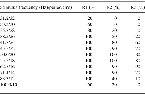
As noted in the Introduction, the amplitude and timing characteristics of R1 have been reported previously (McAnany & Alexander, Reference McAnany and Alexander2009). R1 is typically observed at stimulus frequencies above 38 Hz, and this response has latency characteristics similar to those of the OSR reported in RGC recordings (Schwartz et al., Reference Schwartz, Harris, Shrom and Berry2007; Schwartz & Berry, Reference Schwartz and Berry2008). Specifically, there is an approximately constant delay between R1 and OS1 across stimulus frequency. As is apparent in Table 1, R2 and R3 occurred over a somewhat narrower range of stimulus frequencies than R1. This table shows the percent of subjects who showed R1, R2, and R3 at the various stimulus frequencies. Whereas the ERGs of all subjects contained R1 over the frequency range from 38.5 through 83.3 Hz, not all subjects showed R2 and R3 components over this range. The present analysis of poststimulus responses was based on ERG recordings obtained at stimulus frequencies for which at least 50% of the subjects had all three response components (i.e., frequencies from 41.7 to 71.4 Hz). The mean values in the figures are based on the data of only those subjects who showed the response component under investigation.
Percent of subjects who had measurable R1, R2, and R3 responses at each of the stimulus frequencies indicated
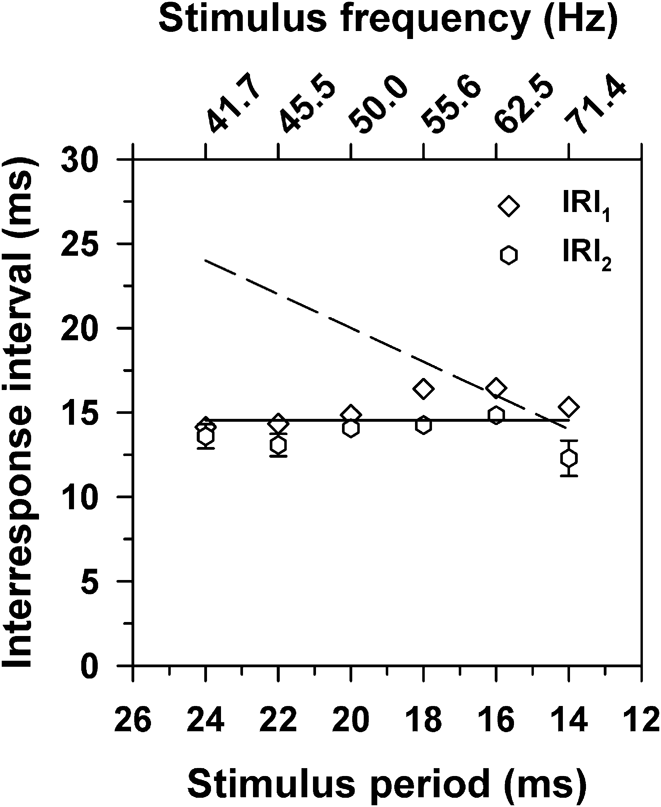
It is apparent from Fig. 1 that both IRI1 and IRI2 were slightly shorter than the stimulus period at this stimulus frequency of 50 Hz. To examine the relationship between IRI and stimulus period further, the mean values of IRI1 and IRI2 across subjects were obtained at each stimulus frequency, with the results plotted in Fig. 2. The dashed line in this figure represents the result to be expected if the IRIs were based on the stimulus period. That is, the dashed line is the result predicted if the poststimulus responses represent a continuing response to the terminated flicker train. The data clearly do not conform to that prediction. Instead, there was a nearly constant IRI across frequency for both intervals.
Mean values of IRI1 (diamonds) and IRI2 (hexagons) as a function of the stimulus period. Error bars in this and the following figures represent ±1 standard error of the mean (s.e.m.) and are omitted when smaller than the symbols. The solid line has a slope of zero and passes through the grand IRI mean. The dashed line represents the IRIs that correspond to the stimulus periods.
There was a tendency for IRI2 to be slightly shorter than IRI1, particularly at short stimulus periods (high frequencies). However, the differences between IRI1 and IRI2 were not statistically significant according to t-tests with a Bonferroni correction for multiple comparisons [t = 0.11 (41.7 Hz), 1.37 (45.5 Hz), 1.48 (50.0 Hz), 3.75 (55.5 Hz), 3.65 (62.5 Hz), 3.96 (71.4 Hz); all P ≥ 0.05]. In addition, the slopes of regression lines that were fit separately to IRI1 and IRI2 were not significantly different from zero (−0.20, P = 0.10; 0.01, P = 0.90; respectively). To characterize the overall tendency of the data, a line of zero slope passing through the grand mean of the IRIs was fit to the data, represented by the solid line in Fig. 2. The grand mean of the IRIs was 14.4 ms, corresponding to a frequency of 69.4 Hz.
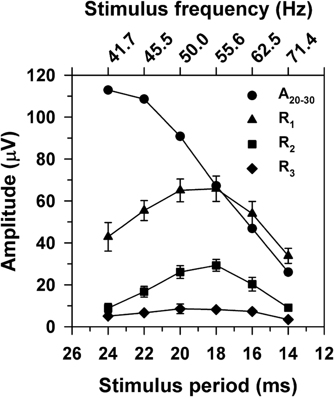
Fig. 3 plots the mean peak-to-trough amplitudes of R1, R2, and R3 as a function of the stimulus period. The amplitude function for R1 was band-pass with a peak near 50 Hz, as reported previously (McAnany & Alexander, Reference McAnany and Alexander2009). The amplitude functions for R2 and R3 were also band-pass, with peaks near 50 Hz, as for R1. Also shown in Fig. 3 are the mean peak-to-trough amplitudes of the flicker ERG (labeled A20–30), defined as the mean of the response amplitudes near the middle of the flicker trains (i.e., stimulus cycles 20 through 30). This cycle range was chosen in order to avoid onset and offset transients and also to provide averages with the same number of cycles across stimulus frequency. In comparison to the results for R1, R2, and R3, the function for A20–30 showed a decreasing amplitude with increasing stimulus frequency.
Mean peak-to-trough amplitudes of R1 (triangles), R2 (squares), R3 (diamonds), and A20–30 (circles) as a function of the stimulus period, where A20–30 represents the mean peak-to-trough ERG amplitude across response cycles 20 through 30.
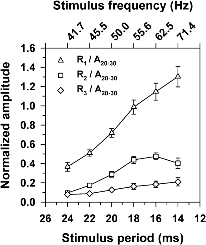
It is likely that the signals that govern the amplitudes of the poststimulus responses are proportional to the overall ERG amplitude, which declines across frequency, as shown in Fig. 3. Therefore, a more meaningful representation of the amplitude characteristics of R1, R2, and R3 is to plot their amplitudes with respect to the amplitude of A20–30 at the same stimulus frequency. Fig. 4 plots the amplitudes of the poststimulus responses normalized in this way. It is apparent from this figure that the relative amplitudes of R1, R2, and R3 actually increased with increasing temporal frequency. These normalized amplitudes were then used in the modeling described in the following section.
Mean amplitudes of R1 (triangles), R2 (squares), and R3 (diamonds) as a function of the stimulus period, with amplitudes normalized to A20–30.
Modeling the poststimulus responses using a resonant system
The approximately constant delay between the poststimulus responses at all stimulus frequencies (Fig. 2) together with the declining amplitude across R1, R2, and R3 (Fig. 3) suggest that a resonant mechanism may be responsible for the generation of the poststimulus responses. If that is the case, then the amplitude characteristics of the poststimulus responses should be well-described by a mathematical model of a resonant system, such as an LRC circuit that has been used previously to describe resonances in retinal ON bipolar cells (Gao et al., Reference Gao, Schwartz, Berry and Holmes2009). The response of such a resonant system can be described using the equation for a forced oscillator:
 $${{\rm{d}}^2}(x)/{\rm{d}}{t^2} + 2\zeta {\omega _0}{\rm{d}}(x)/{\rm{d}}t + {\omega _{\rm{0}}}^2(x) = a\sin ({\omega _1}t),$$$$
in which the sinusoidal waveform on the right side of eqn. (1) represents the driving stimulus, with angular frequency ω 1 and amplitude α. The response to the stimulus is a function of the natural resonant frequency (ω 0) and the damping factor (ζ) of the system. The natural resonant frequency is the frequency at which the system oscillates in the absence of any external stimulus following a disturbance from its equilibrium. The damping factor describes the rate at which the system oscillations decay.
To determine if eqn. (1) describes the amplitude characteristics of the poststimulus responses adequately, estimates for the parameters ω 0 and ζ were derived from the data obtained in response to the 50-Hz stimulus (i.e., near the peak of the amplitude functions for the poststimulus responses shown in Fig. 3). These parameter estimates were then used in eqn. (1) to derive the predicted responses to other stimulus frequencies between 38.5 and 100 Hz.
In order to derive ζ, the natural logs of the amplitude ratios of R2 to R1 and R3 to R2 were first obtained for each subject from the responses to the 50-Hz stimulus. The means across subjects (±1 standard deviation; s.d.) for the log amplitude ratios for R2/R1 and R3/R2 were −0.95 ± 0.39 and −1.05 ± 0.56, respectively. These values did not differ significantly (t = 1.14, P = 0.29), so they were averaged for each subject to give the mean ratio (δ) for that subject. The relationship between ζ and δ is given by:
 $$\zeta = \delta /\sqrt {({{(2\pi )}^2} + {\delta ^2})} .$$
The value of ζ was derived for each subject using eqn. (2). The overall mean value of ζ across subjects (±1 s.d.) was 0.15 ± 0.05.
The value of ω 0 was derived as follows. First, an estimate of the damped resonance frequency (ω d) for each subject was derived from the reciprocal (in Hz) of the mean IRI (in s) obtained from the ERG response to the 50-Hz stimulus. The mean value of ω d (±1 s.d.) across subjects was 69.4 ± 4.1 Hz. Then the value of ω 0 was derived from the estimates of ω d and ζ using the following relationship:
 $${\omega _{\rm{0}}}{\rm{ = }}{\omega _{\rm{d}}}{\rm{/}}\sqrt {{\rm{(1}} - 2{\zeta ^2})} .$$
Across subjects, the mean value of ω 0 (±1 s.d.) was 70.3 ± 4.2 Hz, which is not very different from ω d (69.4 ± 4.1), as would be expected for a resonant system with a low damping constant (ζ = 0.15).
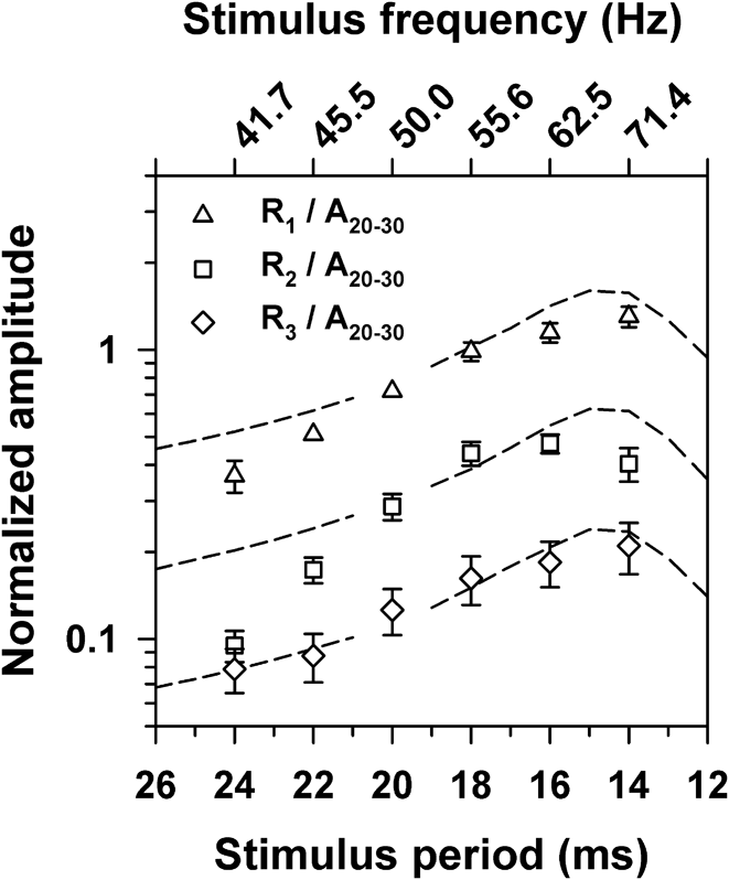
The means across subjects for the parameter estimates for ω 0 and ζ were then used in eqn. (1) to simulate responses to sine waves that had an amplitude of 1 and stimulus periods that ranged from 26 to 12 ms (38.4 to 83.3 Hz) in 1-ms steps, using Simulink (MathWorks, Inc., Natick, MA). The peak-to-trough amplitudes of the first, second, and third extra responses in the simulation output were then obtained. Fig. 5 presents the amplitudes of the simulation output across stimulus period versus the normalized amplitudes of R1, R2, and R3, replotted from Fig. 4. The simulation amplitudes were scaled vertically as a group to minimize the difference between their log amplitudes and the corresponding normalized log ERG amplitudes at 50 Hz. The normalized amplitudes were plotted on a log y-axis to emphasize the exponential decline in amplitude across R1, R2, and R3.
Mean normalized ERG amplitudes (symbols) as a function of the stimulus period, replotted from Fig. 4 on a log y-axis. Dashed lines represent amplitudes derived from the simulation, scaled vertically as a group to provide the least-squares best-fit to the mean log ERG amplitudes at 50 Hz.
The simulation predicted a maximum amplitude for R1, R2, and R3 near the damped resonant frequency ω d (69.4 Hz), which is close to the peaks of the actual ERG amplitudes. Moreover, the simulation predicted an exponential decline in amplitude from R1 to R2 to R3, as represented by the equal vertical spacing between the dashed curves on this log-linear plot. It is apparent that the ERG amplitudes also showed such an exponential decline.
Discussion
Multiple poststimulus responses can be observed in the human cone flicker ERG at stimulus frequencies between approximately 40 and 70 Hz (Fig. 1 and Table 1). The purpose of the present study was to determine whether these poststimulus responses represent a continuing response to the terminated flicker train or are due to a resonant mechanism. Our results support the latter possibility. The IRIs between R1, R2, and R3 were approximately constant across stimulus frequency (Fig. 2) rather than having the proportional relationship to stimulus period that would be expected if they were a continuing response to the flicker train.
Moreover, the amplitude characteristics of the poststimulus responses of the flicker ERG are well described by a mathematical model of a simple resonance system, as illustrated in Fig. 5. The resonance model employed in the present study predicts that the amplitudes of the poststimulus responses should be greatest near the resonance frequency, as shown by the dashed lines in Fig. 5. The model also predicts that the amplitudes of the poststimulus responses should decline exponentially over time following stimulus termination, as illustrated by the constant spacing between the predicted functions for R1, R2, and R3 on the log y-axis of this figure. The ERG data shown in Fig. 5 are consistent with these predictions. Therefore, the temporal sequence of R1, R2, and R3 appears to be a stereotyped response originating from a simple resonance mechanism regardless of stimulus frequency.
An LRC resonant circuit model similar to the one used in the present study was employed previously to describe the poststimulus response (i.e., OSR) recorded from RGCs of salamander and mouse (Gao et al., Reference Gao, Schwartz, Berry and Holmes2009). However, in contrast to our simplified resonance model [eqn. (1)], the model of Gao et al. (Reference Gao, Schwartz, Berry and Holmes2009) incorporated an adaptive mechanism by which the resonance is tuned to the stimulus frequency. This adaptive mechanism was included in order to account for the latency properties of the RGC OSR. As noted in the Introduction, the first poststimulus response of the human ERG (R1) has timing properties that are similar to those of the RGC OSR. Specifically, there is an approximately constant delay between R1 and OS1 over the stimulus frequency range of approximately 38 to 63 Hz. Our resonance model could be expanded to incorporate the OSR-like properties of this first poststimulus response, but this was beyond the scope of the present study. However, we note that our simplified model is able to describe adequately the amplitude and timing characteristics of the poststimulus responses R2 and R3 with respect to R1, which was the focus of our investigation.
Schwartz and Berry (Reference Schwartz and Berry2008) proposed that the RGC OSR is generated by an intrinsic resonance in retinal ON bipolar cells, noting that spontaneous oscillations have been observed previously in depolarizing (ON) bipolar cells of the goldfish retina (Burrone & Lagnado, Reference Burrone and Lagnado1997). In pharmacological manipulations, Schwartz and Berry (Reference Schwartz and Berry2008) found that blocking ON bipolar cell activity by the administration of the mGluR6 antagonist L-AP4 eliminated the OSR in RGC recordings, whereas GABA, glycine, and acetylcholine signaling from amacrine cells did not appear to play a role in its generation. Based in part on these observations, Gao et al. (Reference Gao, Schwartz, Berry and Holmes2009) proposed that the bipolar cell terminal contains an LRC oscillator that produces ringing for one or more periods following stimulus termination, whereas hyperpolarizing or OFF bipolar cells are silent during this period. The RGC OSR would then represent the summation of the responses of ON and OFF bipolar cells.
There is suggestive evidence that the ON bipolar cell pathway may also play an important role in generating the poststimulus responses in the human cone flicker ERG. Specifically, an individual who has the complete form of congenital stationary night blindness (CSNB) due to a NYX gene mutation completely lacked the normal poststimulus ERG responses (McAnany et al., Reference McAnany, Alexander, Kumar, Ying, Anastasakis and Fishman2013). In this form of CSNB, there is an apparent defect in signal transmission from photoreceptors to ON bipolar cells.
In summary, at high temporal frequencies, the human cone flicker ERG contains extra response cycles that occur following the termination of a flicker train. Our analysis of these poststimulus responses indicates that they are likely generated by an underlying resonant circuit with a resonance peak at approximately 70 Hz. Electrophysiological recordings from various species suggest that the poststimulus responses may depend in large part on a resonant mechanism involving retinal ON bipolar cells. If that is the case, then the measurement of these poststimulus responses in the human cone flicker ERG may provide a useful tool to investigate the integrity of resonance mechanisms within the retinal ON pathway. However, further investigation is required to identify the specific neural mechanisms that generate the poststimulus responses observed in the human cone flicker ERG.
Acknowledgment
This research was supported by NIH research grants R01EY008301 (KRA) and R00EY019510 (JJM), NIH ARRA grant 3R01EY008301-18S1 (KRA), NIH core grant P30EY001792, and an unrestricted departmental grant from Research to Prevent Blindness. The authors thank Santosh Balakrishnan for assistance in implementing the mathematical modeling.