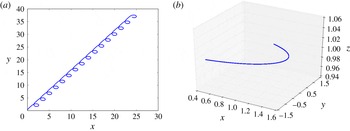
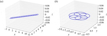
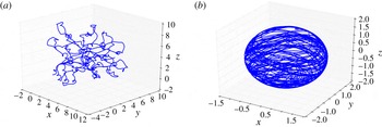
1 Introduction
Ever since the early work of Lighthill (Reference Lighthill1952) and others (Purcell Reference Purcell1952; Blake Reference Blake1971), the self-propulsion of micro-organisms has attracted a great deal of interest (for an early review, see Lighthill Reference Lighthill1976). Over the last 10 years or so, the activity has increased enormously, partially motivated by the successful design of artificial swimmers. Both biological and artificial micro-swimmers have now been studied extensively (Lauga & Powers Reference Lauga and Powers2009; Ebbens & Howse Reference Ebbens and Howse2010; Elgeti, Winkler & Gompper Reference Elgeti, Winkler and Gompper2015; Maass et al. Reference Maass, Krüger, Herminghaus and Bahr2016), both experimentally and with the help of analytical modelling and simulation.
In the world of living micro-organisms, there are many specific examples of self-propelled motion. One possibility is controlled shape changes of the organism as the cause of self-propulsion. These changes may either occur on the scale of the whole system, like in amoeboid or flagella-driven motion, or they may be confined to a thin boundary layer at the interface, like in ciliar motion of micro-organisms. On the other hand, many artificial systems have been fabricated, allowing for a high degree of control of the mechanisms of self-propulsion and the resulting dynamics of single swimmers as well as collective motion (Bechinger et al. Reference Bechinger, Leonardo, Löwen, Reichhardt, Volpe and Volpe2016). Common mechanisms are based on chemical reactions on the surface of the swimmer (Golestanian, Liverpool & Adjari Reference Golestanian, Liverpool and Adjari2005; Takabatake et al. Reference Takabatake, Magome, Ichikawa and Yoshikawa2011; Peddireddy et al. Reference Peddireddy, Kumar, Thutupalli, Herminghaus and Bahr2012; Herminghaus et al. Reference Herminghaus, Maas, Krüger, Thutupalli, Goering and Bahr2013) and, more generally, phoretic effects (Golestanian, Liverpool & Adjari Reference Golestanian, Liverpool and Adjari2007; Herminghaus et al. Reference Herminghaus, Maas, Krüger, Thutupalli, Goering and Bahr2013). In addition, biomimetic devices have been assembled and analysed, such as solutions of cytoskeletal filaments and motors (Köhler, Schaller & Bausch Reference Köhler, Schaller and Bausch2011; Sanchez et al. Reference Sanchez, Chen, DeCamp, Heymann and Dogic2012).
For an important class of micro-swimmers, including micro-organisms, active flow and self-propulsion are generated by energy conversion processes, which produce forces inside the swimmer or at its boundary. From the point of view of fluid mechanics at low Reynolds number, it is sufficient to know the actively generated flow field on the boundary to calculate the flow field in the ambient fluid, and from that extract the self-propulsion of the swimmer. However, for a complete understanding of the system, one should relate this active boundary flow to the energy conversion and force generating processes inside the swimmer. For some artificial micro-swimmers – for example those driven by the Marangoni effect – this is possible (Schmitt & Stark Reference Schmitt and Stark2013, Reference Schmitt and Stark2016). For micro-organisms, however, this is a demanding task due to the complex chemical and mechanical properties of a biological cell. Our work aims to establish a link between the trajectory of a swimmer and its force generating mechanism located inside the swimmer or at its boundary.
For organisms that possess specialised organelles for motility like flagella or cilia, much work has been carried out to link the motion of the organelles to both self-propulsion and cellular active processes. In the case of bacterial flagella, both such links have been established (Berg Reference Berg2003; Lauga Reference Lauga2016). For ciliated organisms, squirmer models constitute an important step towards a complete understanding. These models determine a boundary layer flow resulting from the synchronised motion of cilia, and use it as a boundary condition for internal and ambient creeping flow(Lighthill Reference Lighthill1952; Blake Reference Blake1971). It is known that the cilia are set into motion by molecular motors, but the synchronisation of the motion – giving rise to metachronal waves – is not well understood. Other micro-organisms, like, for example, the cyanobacterium Synechococcus or Myxobacteria, do not possess external organelles associated with motility, but are driven by motors, which produce helical mechanical waves at the internal side of the cell membrane (Nan et al. Reference Nan, Chen, Neu, Berry, Oster and Zusman2001; Ehlers & Oster Reference Ehlers and Oster2012).
Active molecular motors are found at many other places in biological cells, where they exert forces on the intracellular medium, causing changes in pressure and cytoplasmic streaming. The motion of molecular motors and attached cargos or fibres creates complex intra- and extracellular flow patterns as well as membrane bound flows at vesicular boundaries. For some systems, the biological functions of intracellular flow and pressure changes are obvious. In large cells, for example, they are necessary to carry nutrients and signals, which would be much too slow if transported by diffusion (Goldstein Reference Goldstein2016). An example of intracellular pressure differences related to biological function is the creation of blebs (Strychalski & Guy Reference Strychalski and Guy2016). However, very little is known about the effects of cytoplasmic streaming as a mechanism for self-propulsion.
Theoretical modelling is hampered by the fact that intracellular motion at the smallest scales poses highly non-trivial problems of cytosolic flow interacting with a heterogeneous structure exhibiting complex visco-elastic behaviour. On a mesoscopic hydrodynamic level, the internal mechanical properties of cells have been modelled as material continua (Dembo & Harlow Reference Dembo and Harlow1986; Ateshian & Humphrey Reference Ateshian and Humphrey2012) in many ways, with a distribution of active force densities or stress tensors (Joanny et al. Reference Joanny, Jülicher, Kruse and Prost2007), which are generated by molecular motors and (dis)-assembly of semi-flexible polymers (Loisel et al. Reference Loisel, Boujemaa, Pantaloni and Carlier1999). However, even these simplified homogenised models lead to complicated nonlinear field equations, which have to be studied numerically, except in some special simple situations.
To make further progress in understanding the links between active cell mechanics, self-propulsion of organisms and flow fields inside and outside of micro-organisms, one can turn to detailed computer models of molecular processes and structures. Alternatively, one can try to gain insights from simplified hydrodynamic models, which allow for an exact solution in closed analytic form, and yet capture some of the structural properties of micro-organisms and allow one to connect microscopic models of force generation to fluid dynamics. In the present work, we follow the second strategy. In a first part, we calculate the flow fields generated by given active body force densities, surface force densities (tractions) or active stress distributions of a spherical droplet at one instant of time in the limit of vanishing Reynolds number, using a mode expansion into vector spherical harmonics. In particular, we focus on the generated velocities of self-propulsion. The detailed forms of the forces or stresses have to be provided by models of force generating mechanisms, but as the motion of the droplet is entirely determined by only a few terms of the mode expansion, many details of the forces and stresses are not significant for self-propulsion. We demonstrate this reduction explicitly, by studying an example of a stress distribution that may arise in a polar active medium. In a second part, we construct the trajectories of the droplet in a quasisteady-state approximation. Time dependences of the velocities result from time-dependent force distributions in the laboratory frame. To set up an evolution equation of forces, one has to introduce the internal structure of the droplet, which carries the active forces or stresses. We study the case of a sparse rigid statistically isotropic structure (rigid active matter) immersed in a Newtonian fluid. This model possesses a simple and intuitive evolution of force densities in the laboratory frame. Such a structure may be interpreted as a first approximation of stable microtubules. Within this model, we relate time-dependent features of active force distributions to specific classes of trajectories.
The flow fields both outside and inside of micro-organisms have been observed (Mustacich & Ware Reference Mustacich and Ware1976; Drescher et al. Reference Drescher, Goldstein, Michel, Polin and Tuval2010). We therefore also compute these flow fields in the mode expansion, and present the complete solution in appendix A. These results complement and supplement the results of Ghose & Adhikari (Reference Ghose and Adhikari2014) for active particles, which were obtained in terms of a Cartesian multipole expansion.
The paper is organised as follows. In § 2, we introduce the model, specify the boundary conditions and set up the general solution strategy. In § 3, we discuss the flow fields of surface tractions, connect the force- and torque-free case to the squirmer, and show that forces that can be derived from a potential are equivalent to given surface tractions. In § 4, we discuss a general class of active force densities in the interior of the droplet, and in § 5, we consider the case of active stresses, which are generated by a polar medium. All calculations and results of §§ 3–5 refer to a single instant in time and therefore need no evolution equation of the active material. In § 6, we discuss the coupled dynamics of rigid active matter and internal flow, and discuss some illustrating cases of emerging trajectories, before ending with conclusions and an outlook in § 7. Details of the calculations are assigned to appendix A.
2 Model
Embedded within a Newtonian fluid, consider a droplet of another viscous fluid, which at time
 $t$
occupies a finite region
 $K(t)$
in three-dimensional space. The two fluids differ in viscosity and are assumed to be incompressible and completely immiscible. Inside the droplet or located at its geometric boundary
 $\unicode[STIX]{x2202}K(t)$
, we assume active force densities, and we want to study how they lead to self-propulsion of the droplet in a regime of negligible Reynolds number (Happel & Brenner Reference Happel and Brenner1983; Kim & Karrila Reference Kim and Karrila2005). In a first step, we consider the forces as given. In a second step, which will be discussed in detail in § 6, we study the coupled dynamics of flow and active forces carried by a rigid (cyto)-skeleton within the droplet. We restrict the class of systems under study to spherical droplets (of fixed radius
 $a$
), which do not change their shape during time evolution. The field of normal unit vectors on
 $\unicode[STIX]{x2202}K$
thus consists of radial unit vectors
 $\boldsymbol{e}_{r}$
pointing into the ambient fluid.
At every fixed instant of time, the flow velocity fields
 $\boldsymbol{v}^{\pm }$
inside (
 $-$
) and outside (
 $+$
) the droplet have to obey the Stokes equations in the laboratory frame,
 $$\begin{eqnarray}\unicode[STIX]{x1D702}^{\pm }\unicode[STIX]{x1D6FB}^{2}\boldsymbol{v}^{\pm }-\unicode[STIX]{x1D735}p^{\pm }=\unicode[STIX]{x1D735}\boldsymbol{\cdot }\unicode[STIX]{x1D748}^{\pm }=-\boldsymbol{f}^{\,act}-\boldsymbol{f}^{ext},\quad \unicode[STIX]{x1D735}\boldsymbol{\cdot }\boldsymbol{v}^{\pm }=0,\end{eqnarray}$$
with viscosity
 $\unicode[STIX]{x1D702}^{\pm }$
inside and outside of the droplet. The flow fields
 $\boldsymbol{v}^{\pm }$
create viscous stresses
 $\unicode[STIX]{x1D748}^{\pm }$
with Cartesian components
 $\unicode[STIX]{x1D70E}_{ij}^{\pm }=-p^{\pm }\unicode[STIX]{x1D6FF}_{ij}+\unicode[STIX]{x1D702}^{\pm }(\unicode[STIX]{x2202}_{j}v_{i}^{\pm }+\unicode[STIX]{x2202}_{i}v_{j}^{\pm })$
, where
 $\unicode[STIX]{x2202}_{i}v_{j}$
denotes the partial derivative
 $\unicode[STIX]{x2202}v_{j}/\unicode[STIX]{x2202}x_{i}$
. The pressure fields
 $p^{\pm }$
are fixed by the incompressibility condition up to a constant. The active force density,
 $\boldsymbol{f}^{\,act}$
, vanishes outside of the droplet. We can either prescribe the force density or an active stress, which uniquely determines
 $\boldsymbol{f}^{\,act}=-\unicode[STIX]{x1D735}\boldsymbol{\cdot }\unicode[STIX]{x1D748}^{act}$
. It should be noted, however, that the reverse is not true. Generally, it is not possible to calculate a unique stress from a body force density by solving
 $-\unicode[STIX]{x1D735}\boldsymbol{\cdot }\unicode[STIX]{x1D748}^{act}=\boldsymbol{f}^{\,act}$
without any further information about the underlying molecular interactions. For the purposes of our general framework, we therefore treat the problems of given
 $\boldsymbol{f}^{\,act}$
and given
 $\unicode[STIX]{x1D748}^{act}$
separately. We have also introduced an external body force density
 $\boldsymbol{f}^{ext}$
for later use.
To determine
 $\boldsymbol{v}^{\pm }$
uniquely, the Stokes equations have to be supplemented by boundary conditions at the interface and at infinity. There are two boundary conditions at
 $\unicode[STIX]{x2202}K(t)$
. First, we use the assumption that there is no velocity slip, i.e. the tangential velocity component is continuous across the interface. In combination with the condition of immiscibility, this leads to the continuity of
 $\boldsymbol{v}$
across
 $\unicode[STIX]{x2202}K(t)$
,
 $$\begin{eqnarray}\boldsymbol{v}^{+}(\boldsymbol{r})=\boldsymbol{v}^{-}(\boldsymbol{r})\quad \text{for}~\boldsymbol{r}\in \unicode[STIX]{x2202}K(t).\end{eqnarray}$$
The second boundary condition at
 $\unicode[STIX]{x2202}K(t)$
simply states that the interface is free, i.e. all forces acting on each area element must add up to zero. The viscous tractions
 $\boldsymbol{t}^{\pm }=\pm \boldsymbol{e}_{r}\boldsymbol{\cdot }\unicode[STIX]{x1D748}^{\pm }$
, which act on
 $\text{d}^{2}\boldsymbol{S}=\text{d}^{2}S\,\boldsymbol{e}_{r}$
at the interface, are balanced by a variety of forces, from which we separate a ubiquitous Laplace pressure term
 $\boldsymbol{t}_{L}=-\unicode[STIX]{x1D6FE}_{0}(\unicode[STIX]{x1D735}\boldsymbol{\cdot }\boldsymbol{e}_{r})\boldsymbol{e}_{r}=-(2\unicode[STIX]{x1D6FE}_{0}/a)\boldsymbol{e}_{r}$
resulting from a homogeneous surface tension
 $\unicode[STIX]{x1D6FE}_{0}$
, so that
 $\boldsymbol{t}^{+}+\boldsymbol{t}^{-}+\boldsymbol{t}_{L}+\boldsymbol{t}_{a}=0$
on
 $\unicode[STIX]{x2202}K(t)$
. If the active stress,
 $\unicode[STIX]{x1D748}^{act}$
is non-vanishing at the interface, it will also contribute to
 $\boldsymbol{t}_{a}$
. We separate this term explicitly and write
 $\boldsymbol{t}_{a}=-\boldsymbol{e}_{r}\boldsymbol{\cdot }\unicode[STIX]{x1D748}^{act}|_{\unicode[STIX]{x2202}K}+\boldsymbol{t}^{\,act}$
. The boundary condition then takes on the form
 $$\begin{eqnarray}\boldsymbol{e}_{r}\boldsymbol{\cdot }(\unicode[STIX]{x1D748}^{+}-\unicode[STIX]{x1D748}^{-})=\frac{2\unicode[STIX]{x1D6FE}_{0}}{a}\boldsymbol{e}_{r}+\boldsymbol{e}_{r}\boldsymbol{\cdot }\unicode[STIX]{x1D748}^{act}-\boldsymbol{t}^{\,act}\quad \text{on}~\unicode[STIX]{x2202}K(t).\end{eqnarray}$$
We do not consider any ambient background flow in the laboratory frame (LF); hence, the velocity should vanish for
 $|\boldsymbol{r}|\rightarrow \infty$
, and the total force acting on the surface of an infinitely large sphere should stay finite. This requires
 $\boldsymbol{v}^{+}(\boldsymbol{r})=O(1/|\boldsymbol{r}|)$
for
 $|\boldsymbol{r}|\rightarrow \infty$
. The pressure is only determined up to a constant reference, which we fix by
 $p^{+}(\boldsymbol{r})\rightarrow 0$
for
 $|\boldsymbol{r}|\rightarrow \infty$
. For an autonomous swimmer, one furthermore requires that it is force-free, so that momentum is conserved. Therefore, the momentum flux
 $\boldsymbol{J}^{+}(r)=\int _{r}\,\text{d}^{2}S\,\unicode[STIX]{x1D748}^{+}\boldsymbol{\cdot }\boldsymbol{e}_{r}$
through the surface of a sphere of radius
 $r$
vanishes for
 $r\rightarrow \infty$
. The viscous stresses thus have to vanish faster than
 $r^{-2}$
, so that the flow velocity has to vanish faster than
 $r^{-1}$
. This rules out the so-called Stokeslet solutions with
 $\boldsymbol{v}^{+}\propto r^{-1}$
for
 $r\rightarrow \infty$
. For active tractions and body forces, momentum conservation implies the requirement
 $$\begin{eqnarray}\boldsymbol{F}=\int _{\unicode[STIX]{x2202}V}\,\text{d}^{2}S\,\boldsymbol{t}^{\,act}+\int _{V}\,\text{d}V\,\boldsymbol{f}^{\,act}=0\end{eqnarray}$$
as an additional constraint. This constraint is fulfilled automatically if
 $\boldsymbol{f}^{\,act}$
and
 $\boldsymbol{t}^{\,act}$
result from active stresses, because
 $\int _{V}\,\text{d}V\unicode[STIX]{x1D735}\boldsymbol{\cdot }\unicode[STIX]{x1D748}^{act}=0$
due to Gauss’s theorem for any
 $V$
enclosing the droplet.
Similar arguments hold for the torques. For autonomous swimmers, the total torque has to vanish, and the requirement
 $$\begin{eqnarray}\boldsymbol{N}=\int _{\unicode[STIX]{x2202}V}\,\text{d}^{2}S\,\boldsymbol{r}\times \boldsymbol{t}^{\,act}+\int _{V}\,\text{d}V\,\boldsymbol{r}\times \boldsymbol{f}^{\,act}=0\end{eqnarray}$$
is an additional constraint on
 $\boldsymbol{t}^{\,act}$
and
 $\boldsymbol{f}^{\,act}$
. The torque generated by active stresses vanishes automatically if
 $\unicode[STIX]{x1D748}^{act}$
is symmetric.
If additional external fields such as buoyancy due to density mismatch, walls in a micro-fluidic device or optical traps are present, the total momentum is no longer conserved and the momentum sources or sinks resulting from external force densities
 $\boldsymbol{f}_{\!ext}(\boldsymbol{r},t)$
have to be added to the above relations. These force densities are usually specified as functions in the LF.
The translational motion of the droplet is characterised by the velocity
 $\boldsymbol{v}_{CM}$
of its centre of mass, which equals the centre of the sphere. For an incompressible flow,
 $v_{i}=\unicode[STIX]{x2202}(v_{i}x_{j})/\unicode[STIX]{x2202}x_{i}$
, and, consequently,
 $\boldsymbol{v}_{CM}$
can be expressed as an integral over the interface as follows:
 $$\begin{eqnarray}\boldsymbol{v}_{CM}(t)=\frac{3}{4\unicode[STIX]{x03C0}a^{3}}\int _{K}\boldsymbol{v}^{-}\,\text{d}V=\frac{3}{4\unicode[STIX]{x03C0}a^{2}}\int _{\unicode[STIX]{x2202}K(t)}(\boldsymbol{v}^{\pm }\boldsymbol{\cdot }\boldsymbol{e}_{r})\boldsymbol{e}_{r}\,\text{d}^{2}S.\end{eqnarray}$$
An angular velocity may be defined analogously as the total angular momentum divided by the moment of inertia
 $I=8\unicode[STIX]{x03C0}a^{5}/15$
of the homogeneous spherical droplet,
 $$\begin{eqnarray}\unicode[STIX]{x1D74E}=\frac{1}{I}\int _{K}\boldsymbol{r}\times \boldsymbol{v}^{-}\,\text{d}V.\end{eqnarray}$$
The significance of this
 $\unicode[STIX]{x1D74E}$
for the trajectories of the droplet will be discussed in § 6.
Our general strategy for studying self-propulsion consists of two steps. First, the boundary value problem posed by (2.1)–(2.3) is solved at a fixed instant of time in a spherical coordinate system with its origin at the centre of the sphere. We expand all quantities in terms of scalar or vector spherical harmonics, each characterised by a set of integer numbers
 $0\leqslant \ell <\infty$
and
 $-\ell \leqslant m\leqslant \ell$
. The definitions of the vector spherical harmonics and details of the solution procedure can be found in appendix A. The Stokes equations become a system of uncoupled ordinary differential equations for the mode amplitudes with fixed
 $\ell$
and
 $m$
. The rigid body motions of the droplet are exclusively contained in the
 $\ell =1$
modes, which, for self-propelling droplets, contribute a term
 $O(r^{-3})$
to
 $\boldsymbol{v}^{+}$
. The leading contributions
 $\boldsymbol{v}^{+}=O(r^{-2})$
for large
 $r$
emerge from
 $\ell =2$
modes, and some of the
 $\ell =3$
modes also decay as
 $O(r^{-3})$
. Thus, reduced descriptions of the force densities in terms of vector multipoles with
 $\ell =1,2$
and 3 are sufficient, if one is only interested in the trajectories of the droplets and the far field of the accompanying flow. In the present work, we will focus on the droplet motion. Therefore, in a second step, we determine the temporal evolution of active forces in a simple model of rigid active matter and construct the common translational motion of the droplet and the rigid skeleton, and the rotational motions of these two constituents.
3 Activity generated by traction forces
In this section, we consider a droplet with given active tractions,
 $\boldsymbol{t}^{\,act}$
, on its surface. It is our goal to compute the external,
 $\boldsymbol{v}^{+}$
, and internal,
 $\boldsymbol{v}^{-}$
, flow fields as well as the centre of mass velocity,
 $\boldsymbol{v}_{CM}$
, and the rotational velocity,
 $\unicode[STIX]{x1D74E}$
, of the droplet in terms of vector multipole moments of
 $\boldsymbol{t}^{\,act}$
. We first consider general tractions, exerting a non-zero force and torque on the droplet. Subsequently, we specialise to the force- and torque-free case, i.e. we discuss an autonomous swimmer that is propelled by surface tractions. We compare our results with the well-studied squirmer with an active flow prescribed on the surface. The linear velocity and the external flow can be mapped onto each other, whereas the rotational velocity of the droplet driven by tractions vanishes. The droplet furthermore develops a characteristic flow pattern in the interior, and energy is dissipated by both the interior and the exterior flow, with the ratio of the two determined by the corresponding ratio of viscosities. We also show that external forces that can be derived from a potential, such as gravity, can be mapped onto tractions. The motion of the droplet with active tractions and external force is worked out.
3.1 General tractions
To determine the droplet trajectories, we start from the
 $\ell =1$
modes of active tractions (see appendix A) at a fixed time
 $t$
, which we write as
 $$\begin{eqnarray}\boldsymbol{t}_{(\ell =1)}^{\,act}(\unicode[STIX]{x1D703},\unicode[STIX]{x1D711})=\mathop{\sum }_{m=-1}^{1}(\unicode[STIX]{x1D6FC}_{m}Y_{1m}(\unicode[STIX]{x1D703},\unicode[STIX]{x1D711})\boldsymbol{e}_{r}+\unicode[STIX]{x1D6FD}_{m}\unicode[STIX]{x1D735}_{s}Y_{1m}(\unicode[STIX]{x1D703},\unicode[STIX]{x1D711})+\unicode[STIX]{x1D6FE}_{m}\boldsymbol{e}_{r}\times \unicode[STIX]{x1D735}_{s}Y_{1m}(\unicode[STIX]{x1D703},\unicode[STIX]{x1D711})).\end{eqnarray}$$
Here,
 $\unicode[STIX]{x1D735}_{s}$
denotes the angular part of the gradient operator, i.e.
 $\unicode[STIX]{x1D735}_{s}g(\unicode[STIX]{x1D703},\unicode[STIX]{x1D711})=r\unicode[STIX]{x1D735}g(\unicode[STIX]{x1D703},\unicode[STIX]{x1D711})$
. The
 $\ell =1$
part of the active traction field is determined by nine multipole moments
 $\unicode[STIX]{x1D6FC}_{m}$
,
 $\unicode[STIX]{x1D6FD}_{m}$
,
 $\unicode[STIX]{x1D6FE}_{m}$
, which correspond to nine real parameters. For any given traction field, these moments are obtained by projection of
 $\boldsymbol{t}^{\,act}$
onto the corresponding vector spherical harmonics. Higher-
 $\ell$
moments do not contribute to self-propulsion.
We solve the Stokes equations in the interior and exterior regions of the droplet and find for the velocity fields in the LF
 $$\begin{eqnarray}\displaystyle \displaystyle \boldsymbol{v}^{+}(\boldsymbol{r}) & = & \displaystyle \mathop{\sum }_{m}\left(\left(a_{m}^{+}\frac{a}{r}+b_{m}^{+}\frac{a^{3}}{r^{3}}\right)Y_{1m}(\unicode[STIX]{x1D703},\unicode[STIX]{x1D711})\boldsymbol{e}_{r}\right.\nonumber\\ \displaystyle & & \displaystyle \left.+\left(a_{m}^{+}\frac{a}{r}-b_{m}^{+}\frac{a^{3}}{r^{3}}\right)\frac{1}{2}\unicode[STIX]{x1D735}_{s}Y_{1m}(\unicode[STIX]{x1D703},\unicode[STIX]{x1D711})+c_{m}^{+}\frac{a^{2}}{r^{2}}\boldsymbol{e}_{r}\times \unicode[STIX]{x1D735}_{s}Y_{1m}(\unicode[STIX]{x1D703},\unicode[STIX]{x1D711})\right),\end{eqnarray}$$
 $$\begin{eqnarray}\displaystyle \displaystyle \boldsymbol{v}^{-}(\boldsymbol{r}) & = & \displaystyle \mathop{\sum }_{m}\left(\left(a_{m}^{-}\frac{r^{2}}{a^{2}}+b_{m}^{-}\right)Y_{1m}(\unicode[STIX]{x1D703},\unicode[STIX]{x1D711})\boldsymbol{e}_{r}\right.\nonumber\\ \displaystyle & & \displaystyle \left.+\left(2a_{m}^{-}\frac{r^{2}}{a^{2}}+b_{m}^{-}\right)\unicode[STIX]{x1D735}_{s}Y_{1m}(\unicode[STIX]{x1D703},\unicode[STIX]{x1D711})+c_{m}^{-}\frac{r}{a}\boldsymbol{e}_{r}\times \unicode[STIX]{x1D735}_{s}Y_{1m}(\unicode[STIX]{x1D703},\unicode[STIX]{x1D711})\right).\end{eqnarray}$$
The expansion coefficients are determined by the boundary conditions of (2.2), (2.3), as shown in detail in appendix A.2.
The traction forces are of two kinds. The first one corresponds to tractions with
 $\unicode[STIX]{x1D6FE}_{m}=0$
that give rise to a linear velocity of the droplet but no rotational velocity. The centre of mass velocity is determined by the flow field according to (2.6). Straightforward computation yields
 $$\begin{eqnarray}\boldsymbol{v}_{CM}=\sqrt{\frac{3}{4\unicode[STIX]{x03C0}}}h_{0}\boldsymbol{e}_{z}-\sqrt{\frac{3}{2\unicode[STIX]{x03C0}}}\text{Re}(h_{1})\boldsymbol{e}_{x}+\sqrt{\frac{3}{2\unicode[STIX]{x03C0}}}\text{Im}(h_{1})\boldsymbol{e}_{y},\end{eqnarray}$$
with
 $$\begin{eqnarray}h_{m}=\frac{2a}{3\unicode[STIX]{x1D702}^{+}}\frac{\unicode[STIX]{x1D6FC}_{m}(1+\unicode[STIX]{x1D706})+\unicode[STIX]{x1D6FD}_{m}(1+2\unicode[STIX]{x1D706})}{2+3\unicode[STIX]{x1D706}}.\end{eqnarray}$$
Here, the ratio of interior to exterior viscosity has been denoted by
 $\unicode[STIX]{x1D706}=\unicode[STIX]{x1D702}^{-}/\unicode[STIX]{x1D702}^{+}$
. Such tractions can, for example, be generated by Marangoni flow, which is represented by an inhomogeneous surface tension
 $\unicode[STIX]{x1D6FE}(\unicode[STIX]{x1D703},\unicode[STIX]{x1D711})$
. For this example, the tractions are given by
 $$\begin{eqnarray}a\boldsymbol{t}^{\,act}(\unicode[STIX]{x1D703},\unicode[STIX]{x1D711})=2\unicode[STIX]{x1D6FE}(\unicode[STIX]{x1D703},\unicode[STIX]{x1D711})\boldsymbol{e}_{r}+\unicode[STIX]{x1D735}_{s}\unicode[STIX]{x1D6FE}(\unicode[STIX]{x1D703},\unicode[STIX]{x1D711}),\end{eqnarray}$$
and hence cannot give rise to a rotational velocity of the droplet.
The second class of tractions has only
 $\unicode[STIX]{x1D6FE}_{m}\neq 0$
. The internal flow, as given in (3.3), corresponds to rigid body rotation
 $\boldsymbol{v}^{-}(\boldsymbol{r})=\unicode[STIX]{x1D74E}\times \boldsymbol{r}$
, with the rotational velocity given by
 $$\begin{eqnarray}\unicode[STIX]{x1D74E}=\frac{1}{3\unicode[STIX]{x1D702}^{+}}\sqrt{\frac{3}{2\unicode[STIX]{x03C0}}}\left(\text{Re}(\unicode[STIX]{x1D6FE}_{1})\boldsymbol{e}_{x}-\text{Im}(\unicode[STIX]{x1D6FE}_{1})\boldsymbol{e}_{y}-\frac{\unicode[STIX]{x1D6FE}_{0}}{\sqrt{2}}\boldsymbol{e}_{z}\right).\end{eqnarray}$$
3.2 Force- and torque-free case
In this section, we discuss the special case where no external force and no external torque are present, as required for an autonomous swimmer. We first work out the consequences for self-propulsion by tractions and then compare our results with the squirmer model, in which an active velocity on the surface of a particle is described. The squirmer model has been discussed extensively in the literature, mainly for a solid particle.
Vanishing of the torque,
 $\boldsymbol{N}=\int _{\unicode[STIX]{x2202}K(t)}\,\text{d}^{2}S\boldsymbol{r}\times \boldsymbol{t}_{act}=8\unicode[STIX]{x03C0}a^{3}\unicode[STIX]{x1D702}^{+}\unicode[STIX]{x1D74E}=0$
, implies that all
 $\unicode[STIX]{x1D6FE}_{m}=0$
. In other words, tractions cannot generate rotational motion of an autonomous swimmer. Vanishing of the total force,
 $\boldsymbol{F}=\int _{\unicode[STIX]{x2202}K(t)}\,\text{d}^{2}S\boldsymbol{t}_{act}=0$
, implies a restriction on the multipole moments of the traction forces, namely
 $\unicode[STIX]{x1D6FC}_{m}=-2\unicode[STIX]{x1D6FD}_{m}$
. Consequently, the Stokeslet vanishes, i.e.
 $a_{m}^{+}=0$
, and the exterior flow field with
 $\ell =1$
decays as
 $1/r^{3}$
. The flow fields outside and inside the force-free droplet are explicitly given by
 $$\begin{eqnarray}\displaystyle \left.\begin{array}{@{}c@{}}\displaystyle \boldsymbol{v}^{+}(\boldsymbol{r})=\frac{a}{3\unicode[STIX]{x1D702}^{+}(2+3\unicode[STIX]{x1D706})}\mathop{\sum }_{m=-1}^{1}\unicode[STIX]{x1D6FC}_{m}\frac{a^{3}}{r^{3}}\left(Y_{1m}\boldsymbol{e}_{r}-\frac{1}{2}\unicode[STIX]{x1D735}_{s}Y_{1m}\right),\\ \displaystyle \boldsymbol{v}^{-}(\boldsymbol{r})=\frac{a}{2(3\unicode[STIX]{x1D702}^{+}(2+3\unicode[STIX]{x1D706}))}\mathop{\sum }_{m=-1}^{1}\unicode[STIX]{x1D6FC}_{m}\left(\left(5-3\frac{r^{2}}{a^{2}}\right)Y_{1m}\boldsymbol{e}_{r}+(5-6\frac{r^{2}}{a^{2}})\frac{1}{2}\unicode[STIX]{x1D735}_{s}Y_{1m}\right),\end{array}\right\} & & \displaystyle\end{eqnarray}$$
and the centre of mass velocity follows from equations (3.4) and (3.5) or directly from the constant part of the velocity field in the interior of the droplet,
 $$\begin{eqnarray}\boldsymbol{v}_{CM}=\frac{a}{\sqrt{12\unicode[STIX]{x03C0}}(2\unicode[STIX]{x1D702}^{+}+3\unicode[STIX]{x1D702}^{-})}(\unicode[STIX]{x1D6FC}_{0}\boldsymbol{e}_{z}-\sqrt{2}\text{Re}\,\unicode[STIX]{x1D6FC}_{1}\boldsymbol{e}_{x}+\sqrt{2}\text{Im}\,\unicode[STIX]{x1D6FC}_{1}\boldsymbol{e}_{y}).\end{eqnarray}$$
Instead of considering a force-free droplet, one can ask what force is needed to keep the active droplet at rest in the LF. We now set
 $\boldsymbol{v}_{CM}=0$
and compute the stall force,
 $$\begin{eqnarray}\boldsymbol{F}_{stall}=\int _{\unicode[STIX]{x2202}K(t)}(\unicode[STIX]{x1D748}^{+}\boldsymbol{\cdot }\boldsymbol{n})\,\text{d}^{2}S.\end{eqnarray}$$
As one would expect, the stall force is proportional to
 $\boldsymbol{v}_{CM}$
,
 $$\begin{eqnarray}\boldsymbol{F}_{stall}=-\unicode[STIX]{x1D707}\boldsymbol{v}_{CM},\quad \text{with}~\unicode[STIX]{x1D707}=\frac{(1+\unicode[STIX]{x1D706})}{2\unicode[STIX]{x03C0}a(2\unicode[STIX]{x1D702}^{+}+3\unicode[STIX]{x1D702}^{-})}.\end{eqnarray}$$
The mobility
 $\unicode[STIX]{x1D707}$
is seen to depend on both the interior and exterior viscosities. This reflects the fact that traction forces generate active surface velocities that depend on both viscosities. In the limit that the fluid in the interior becomes highly viscous or even solid-like (
 $\lim \unicode[STIX]{x1D702}^{-}\rightarrow \infty$
), the mobility reduces to the one for a solid particle,
 $\unicode[STIX]{x1D707}=1/(6\unicode[STIX]{x03C0}a\unicode[STIX]{x1D702}^{+})$
. In the opposite limit
 $\lim \unicode[STIX]{x1D702}^{-}\rightarrow 0$
, we recover the mobility of a gas bubble,
 $\unicode[STIX]{x1D707}=1/(4\unicode[STIX]{x03C0}a\unicode[STIX]{x1D702}^{+})$
. In between, the mobility increases monotonically.
We now compare our results with the squirmer model, which prescribes the active velocity field on the surface of the sphere (Blake Reference Blake1971),
 $$\begin{eqnarray}\boldsymbol{v}_{act}(\unicode[STIX]{x1D703},\unicode[STIX]{x1D711})=\mathop{\sum }_{m=-1}^{1}(\unicode[STIX]{x1D70C}_{m}\unicode[STIX]{x1D735}_{s}Y_{1m}(\unicode[STIX]{x1D703},\unicode[STIX]{x1D711})).\end{eqnarray}$$
There is no radial component to the active velocity, because we require the shape and size of the droplet to be preserved. The exterior and interior flow fields
 $\boldsymbol{v}^{\pm }(r,\unicode[STIX]{x1D703},\unicode[STIX]{x1D711})$
have to fulfil the following boundary condition in the LF:
 $$\begin{eqnarray}\boldsymbol{v}^{+}(\boldsymbol{r})=\boldsymbol{v}^{-}(\boldsymbol{r})=\boldsymbol{v}_{CM}+\boldsymbol{v}_{act}(\boldsymbol{r})\quad \text{for}~\boldsymbol{r}\in \unicode[STIX]{x2202}K(t).\end{eqnarray}$$
The centre of mass velocity is yet unknown and has to be determined from the vanishing of the total force. Solving the Stokes equation for
 $\boldsymbol{v}^{\pm }$
with the above boundary condition and the requirement of vanishing total force, we reproduce the result of (3.9) for the centre of mass velocity, if we identify the coefficients of the active tractions with those of the active velocity according to
 $$\begin{eqnarray}\unicode[STIX]{x1D70C}_{m}=-\frac{a\unicode[STIX]{x1D6FC}_{m}}{4\unicode[STIX]{x1D702}^{+}+6\unicode[STIX]{x1D702}^{-}}.\end{eqnarray}$$
The rotational motion of a squirmer has been discussed by Pak & Lauga (Reference Pak and Lauga2014) and more recently by Pedley, Brumley & Goldstein (Reference Pedley, Brumley and Goldstein2016). Only the
 $l=1$
component of the active velocity contributes to the rotational velocity of the squirmer and is equivalent to a rigid rotation of the surface with angular velocity
 $\unicode[STIX]{x1D74E}$
, i.e.
 $\boldsymbol{v}_{act}(\unicode[STIX]{x1D703},\unicode[STIX]{x1D711})=a\unicode[STIX]{x1D74E}\times \boldsymbol{e}_{r}$
. The active velocity gives rise to a rotation in the LF which exactly cancels the above rotational component of
 $\boldsymbol{v}_{act}(\unicode[STIX]{x1D703},\unicode[STIX]{x1D711})$
, so that the
 $l=1$
components of the external and internal flow fields are not affected. Rotational components with
 $l>1$
in
 $\boldsymbol{v}_{act}$
do modify the flow fields inside and outside of the droplet, but do not contribute to
 $\unicode[STIX]{x1D74E}$
.
3.3 Energy dissipation
Energy is dissipated by both the exterior and the interior flows,
 $$\begin{eqnarray}\unicode[STIX]{x2202}_{t}E^{\pm }=\int _{V^{\pm }}\,\text{d}^{3}x\,\unicode[STIX]{x1D70E}_{ik}^{\pm }\unicode[STIX]{x2202}_{k}v_{i}^{\pm }=\pm \int _{\unicode[STIX]{x2202}V}\,\text{d}^{2}x\,v_{i}^{\pm }\unicode[STIX]{x1D70E}_{ik}^{\pm }n_{k},\end{eqnarray}$$
where we have used that
 $\unicode[STIX]{x2202}_{k}\unicode[STIX]{x1D70E}_{ik}^{\pm }=0$
and the normal is always defined as pointing outward from the sphere. The second inequality in the above equation just says that the energy dissipated in the volumes
 $V^{\pm }$
is balanced by the energy inflow from the boundary. The latter is more easily computed, and we obtain for the force-free case
 $$\begin{eqnarray}\displaystyle & \displaystyle \unicode[STIX]{x2202}_{t}E^{+}=-\frac{\unicode[STIX]{x1D702}^{+}a^{2}}{(2\unicode[STIX]{x1D702}^{+}+3\unicode[STIX]{x1D702}^{-})^{2}}(\unicode[STIX]{x1D6FC}_{0}^{2}+2|\unicode[STIX]{x1D6FC}_{1}|^{2}), & \displaystyle\end{eqnarray}$$
 $$\begin{eqnarray}\displaystyle & \displaystyle \unicode[STIX]{x2202}_{t}E^{-}=-\frac{3\unicode[STIX]{x1D702}^{-}a^{2}}{(2\unicode[STIX]{x1D702}^{+}+3\unicode[STIX]{x1D702}^{-})^{2}}(\unicode[STIX]{x1D6FC}_{0}^{2}+2|\unicode[STIX]{x1D6FC}_{1}|^{2}), & \displaystyle\end{eqnarray}$$
so that the ratio is independent of the driving amplitudes
 $\{\unicode[STIX]{x1D6FD}_{m}\}$
,
 $$\begin{eqnarray}\unicode[STIX]{x2202}_{t}E^{+}/\unicode[STIX]{x2202}_{t}E^{-}=\frac{2\unicode[STIX]{x1D702}^{+}}{3\unicode[STIX]{x1D702}^{-}}.\end{eqnarray}$$
In the stationary state, the total dissipation is balanced by the energy input due to surface tractions,
 $\unicode[STIX]{x2202}_{t}E^{+}+\unicode[STIX]{x2202}_{t}E^{-}=\unicode[STIX]{x2202}_{t}E^{act}=\int _{\unicode[STIX]{x2202}V}\,\text{d}^{2}xt_{i}^{act}v_{i}$
.
3.4 Sedimenting active droplets
Consider the simple case of a passive droplet in an external potential, which is assumed to be continuous across the interface. For example, if the fluids are not density matched, then buoyancy forces act on the droplet. These can be represented by a potential
 $U=\unicode[STIX]{x0394}\unicode[STIX]{x1D70C}g(z-a)$
for
 $z\leqslant a$
, where
 $\unicode[STIX]{x0394}\unicode[STIX]{x1D70C}$
denotes the difference in density between the inside and outside fluids. We assume that the sedimentation velocity, which is controlled by
 $\unicode[STIX]{x0394}\unicode[STIX]{x1D70C}$
, is sufficiently small, so that it is justified to still work in the limit of vanishingly small Reynolds number.
In the general case, the potential is expanded in spherical harmonics
 $U=\text{const.}+\sum _{m}U_{m}(r)Y_{1m}$
, keeping only
 $l=1$
. In the interior of the droplet, we then have to solve the Stokes equation
 $$\begin{eqnarray}\unicode[STIX]{x1D702}^{-}\unicode[STIX]{x1D6FB}^{2}\boldsymbol{v}^{-}=\unicode[STIX]{x1D735}p^{-}-\boldsymbol{f}_{\!ext}\end{eqnarray}$$
in the presence of an external force
 $\boldsymbol{f}_{\!ext}=\unicode[STIX]{x1D735}U$
. The force derived from a potential can be absorbed by defining an effective pressure
 $p_{eff}=p^{-}-U$
. The effective pressure has to fulfil Laplace’s equation and determines the inhomogeneous solution of the Stokes equation in the same way as does
 $p^{-}$
without external force. The force balance equation for the interface (2.3) involves only the pressure
 $p^{-}$
, and hence the potential
 $U$
is equivalently represented as a traction force according to
 $$\begin{eqnarray}\boldsymbol{t}_{act}(\unicode[STIX]{x1D703},\unicode[STIX]{x1D711})=\mathop{\sum }_{m=-1}^{1}U_{m}(a)Y_{1m}(\unicode[STIX]{x1D703},\unicode[STIX]{x1D711})\boldsymbol{e}_{r}.\end{eqnarray}$$
If there are no active tractions or body forces, we recover the velocity of the sedimenting passive droplet,
 $\boldsymbol{v}_{CM}=\unicode[STIX]{x1D707}\boldsymbol{f}_{\!ext}$
, with the mobility
 $\unicode[STIX]{x1D707}=(1+\unicode[STIX]{x1D706})/(2\unicode[STIX]{x03C0}a\unicode[STIX]{x1D702}^{+}(2+3\unicode[STIX]{x1D706}))$
. In the general case of an active droplet in an external field, the motion is a linear superposition of the velocity generated by the activity and the velocity caused by the external field,
 $$\begin{eqnarray}\boldsymbol{v}_{CM}=\frac{a}{\sqrt{12\unicode[STIX]{x03C0}}(2\unicode[STIX]{x1D702}^{+}+3\unicode[STIX]{x1D702}^{-})}(\unicode[STIX]{x1D6FC}_{0}\boldsymbol{e}_{z}-\sqrt{2}\text{Re}\,\unicode[STIX]{x1D6FC}_{1}\boldsymbol{e}_{x}+\sqrt{2}\text{Im}\,\unicode[STIX]{x1D6FC}_{1}\boldsymbol{e}_{y})+\unicode[STIX]{x1D707}\boldsymbol{f}_{\!ext},\end{eqnarray}$$
so that sufficiently strong activity may turn a sedimenting droplet into a rising one.
3.5 Conclusion: active tractions
We have analysed general active tractions in the interface of the droplet, and related the linear and angular momentum of the droplet to the vector multipole moments of the traction. For an autonomous swimmer, such tractions can only generate translational motion, which is equivalently generated by an active velocity on the surface of the droplet. Energy is dissipated both inside and outside of the droplet, with the ratio being determined by the two viscosities. A sedimenting active droplet is discussed as a simple example for an active swimmer in an external force field.
4 Activity generated by body forces
So far, we have discussed activity that is generated in the interface of the droplet. We now turn to active mechanisms in the inside of the droplet. One can specify either active forces or active stresses in the inside. The latter will be discussed in § 5 in the context of a polar medium that is naturally described in terms of active stresses. Here, we focus on active forces, such as those generated by motors pulling on filaments and thereby generating flow and inhomogeneous pressure. Of course, active forces are related to active stresses by
 $\boldsymbol{f}^{\,act}(\boldsymbol{r})=-\unicode[STIX]{x1D735}\boldsymbol{\cdot }\unicode[STIX]{x1D748}^{act}$
. However, it is not possible to solve this equation uniquely for
 $\unicode[STIX]{x1D748}^{act}$
without using further properties of the stress tensor. The situation is analogous to the problem of determining the electric field
 $\boldsymbol{E}$
from a charge density
 $\unicode[STIX]{x1D70C}$
without using any further properties of
 $\boldsymbol{E}$
. Only after specifying that
 $\unicode[STIX]{x1D735}\times \boldsymbol{E}=0$
does the problem become well posed. Consequently, we treat the cases of given body force densities and active stresses separately.
4.1 A class of body forces
We start from the
 $\ell =1$
part (see appendix A) of a given force density
 $\boldsymbol{f}^{\,act}$
,
 $$\begin{eqnarray}\boldsymbol{f}_{\ell =1}^{act}(r,\unicode[STIX]{x1D703},\unicode[STIX]{x1D711})=\mathop{\sum }_{m=-1}^{1}(\unicode[STIX]{x1D6FC}_{m}(r)Y_{1m}(\unicode[STIX]{x1D703},\unicode[STIX]{x1D711})\boldsymbol{e}_{r}+\unicode[STIX]{x1D6FD}_{m}(r)\unicode[STIX]{x1D735}_{s}Y_{1m}(\unicode[STIX]{x1D703},\unicode[STIX]{x1D711})+\unicode[STIX]{x1D6FE}_{m}(r)\boldsymbol{e}_{r}\times \unicode[STIX]{x1D735}_{s}Y_{1m}(\unicode[STIX]{x1D703},\unicode[STIX]{x1D711})),\end{eqnarray}$$
which is the analogue of (3.1). In the droplet interior, the Stokes equation becomes inhomogeneous,
 $$\begin{eqnarray}\unicode[STIX]{x1D702}^{-}\unicode[STIX]{x1D6FB}^{2}\boldsymbol{v}^{-}=\unicode[STIX]{x1D735}p^{-}-\boldsymbol{f}^{\,act}.\end{eqnarray}$$
Incompressibility requires
 $\unicode[STIX]{x0394}p^{-}=\unicode[STIX]{x1D735}\boldsymbol{\cdot }\boldsymbol{f}^{\,act}$
. The general solution is given as
 $p^{-}=p_{hom}^{-}+p_{inh}^{-}$
as the sum of the general solution,
 $p_{hom}^{-}$
, of the homogeneous equation and a particular solution,
 $p_{inh}^{-}$
, of the inhomogeneous equation. The former has already been constructed in § 3. Similarly, the solution of (4.2) is decomposed into the previously found flow field for vanishing body force,
 $\boldsymbol{v}_{0}^{-}=\boldsymbol{v}^{-}(\,\boldsymbol{f}^{a}=0)$
, and a particular solution,
 $\boldsymbol{w}$
, of the inhomogeneous equation,
 $$\begin{eqnarray}\unicode[STIX]{x1D702}^{-}\unicode[STIX]{x1D6FB}^{2}\mathbf{w}=\unicode[STIX]{x1D735}p_{inh}^{-}-\boldsymbol{f}^{\,act}.\end{eqnarray}$$
To obtain explicit expressions for
 $p_{inh}$
and
 $\boldsymbol{w}$
, we treat a class of body forces,
 $\boldsymbol{f}^{\,act}$
, consisting of linear combinations of power laws
 $\boldsymbol{f}^{\,act}(r,\unicode[STIX]{x1D703},\unicode[STIX]{x1D719})=\sum _{\unicode[STIX]{x1D708}}(r/a)^{\unicode[STIX]{x1D708}}\boldsymbol{f}_{\unicode[STIX]{x1D708}}(\unicode[STIX]{x1D703},\unicode[STIX]{x1D711})$
, which may be adapted to specific situations. Due to the linearity of the problem, we can restrict the discussion to a single power, so that
 $\unicode[STIX]{x1D6FC}_{m}(r)=(r/a)^{\unicode[STIX]{x1D708}}\unicode[STIX]{x1D6FC}_{m}$
,
 $\unicode[STIX]{x1D6FD}_{m}(r)=(r/a)^{\unicode[STIX]{x1D708}}\unicode[STIX]{x1D6FD}_{m}$
and
 $\unicode[STIX]{x1D6FE}_{m}(r)=(r/a)^{\unicode[STIX]{x1D708}}\unicode[STIX]{x1D6FE}_{m}$
. More general solutions are then obtained by superposition.
For
 $\unicode[STIX]{x1D708}\neq 0$
, a special solution of the inhomogeneous equation for the pressure,
 $\unicode[STIX]{x0394}p_{inh}^{-}=\unicode[STIX]{x1D735}\boldsymbol{\cdot }\boldsymbol{f}^{\,act}$
, is given by
 $$\begin{eqnarray}p_{inh}(\boldsymbol{r})=\left(\frac{r}{a}\right)^{\unicode[STIX]{x1D708}+1}\mathop{\sum }_{m}p_{m}Y_{1m},\quad \text{with}~p_{m}=a\frac{(\unicode[STIX]{x1D708}+2)\unicode[STIX]{x1D6FC}_{m}-2\unicode[STIX]{x1D6FD}_{m}}{\unicode[STIX]{x1D708}(\unicode[STIX]{x1D708}+3)}.\end{eqnarray}$$
We substitute this solution into (4.3) and solve for
 $\boldsymbol{w}$
,
 $$\begin{eqnarray}\left(\frac{r}{a}\right)^{-\unicode[STIX]{x1D708}-2}\boldsymbol{w}=\mathop{\sum }_{m}w_{m}\left(Y_{1m}\boldsymbol{e}_{r}+\frac{\unicode[STIX]{x1D708}+4}{2}\unicode[STIX]{x1D735}_{s}Y_{1m}\right)+u_{m}\boldsymbol{e}_{r}\times \unicode[STIX]{x1D735}_{s}Y_{1m},\end{eqnarray}$$
where the coefficients are given by
 $$\begin{eqnarray}\displaystyle \left.\begin{array}{@{}c@{}}\displaystyle w_{m}=\frac{a^{2}}{\unicode[STIX]{x1D702}^{-}}\frac{(\unicode[STIX]{x1D708}+1)p_{m}/a-\unicode[STIX]{x1D6FC}_{m}}{(\unicode[STIX]{x1D708}+2)(\unicode[STIX]{x1D708}+5)},\\ \displaystyle u_{m}=-\frac{a^{2}}{\unicode[STIX]{x1D702}^{-}}\frac{\unicode[STIX]{x1D6FE}_{m}}{(\unicode[STIX]{x1D708}+1)(\unicode[STIX]{x1D708}+4)}.\end{array}\right\} & & \displaystyle\end{eqnarray}$$
After a special solution
 $\boldsymbol{w}$
has been found, the coefficients appearing in the homogeneous solution,
 $\boldsymbol{v}^{+}$
and
 $\boldsymbol{v}_{0}^{-}$
, equations (3.2) and (3.3), are obtained by matching the boundary conditions at
 $r=a$
, requiring continuity of the velocity equation (2.2),
 $\boldsymbol{v}^{+}=\boldsymbol{v}_{0}^{-}+\boldsymbol{w}$
and balance of tractions (2.3). The resulting system of linear equations is solved in appendix A.2 and discussed in the following sections for an autonomous swimmer.
4.2 Force-free translations and torque-free rotations
For an autonomous swimmer, we require that the total force and total torque of the force density given by (4.1) vanish,
 $\boldsymbol{F}=\int \boldsymbol{f}^{\,act}(\boldsymbol{r})\,\text{d}V=0$
and
 $\boldsymbol{N}=\int \boldsymbol{r}\times \boldsymbol{f}^{\,act}(\boldsymbol{r})\,\text{d}V=0$
. If
 $\unicode[STIX]{x1D6FC}_{m}(r)=-2\unicode[STIX]{x1D6FD}_{m}(r)$
, the forces within each radial shell
 $[r,r+\text{d}r]$
are balanced. Let us specialise to this simple case, with
 $\boldsymbol{f}^{\,act}=(r/a)^{\unicode[STIX]{x1D708}}\boldsymbol{f}_{\unicode[STIX]{x1D708}}$
and
 $\unicode[STIX]{x1D6FC}_{m}=-2\unicode[STIX]{x1D6FD}_{m}$
. Consequently, the amplitude of the Stokeslet vanishes. The centre of mass velocity can be calculated from (2.6), which yields
 $$\begin{eqnarray}\displaystyle & \displaystyle \boldsymbol{v}_{CM}=\sqrt{\frac{3}{2\unicode[STIX]{x03C0}}}(-\text{Re}(b_{1}^{+})\boldsymbol{e}_{x}+\text{Im}(b_{1}^{+})\boldsymbol{e}_{y}+b_{0}^{+}/\sqrt{2}\boldsymbol{e}_{z}), & \displaystyle\end{eqnarray}$$
 $$\begin{eqnarray}\displaystyle & \displaystyle b_{m}^{+}=\frac{a^{2}\unicode[STIX]{x1D6FC}_{m}}{3(\unicode[STIX]{x1D708}+5)(2\unicode[STIX]{x1D702}^{+}+3\unicode[STIX]{x1D702}^{-})}. & \displaystyle\end{eqnarray}$$
A balance in each radial shell is not possible for the torque. Therefore, within our class of models, a force density with vanishing total force and torque requires at least a sum of two different powers,
 $\boldsymbol{f}=r^{\unicode[STIX]{x1D708}}\boldsymbol{f}_{\unicode[STIX]{x1D708}}(\unicode[STIX]{x1D703},\unicode[STIX]{x1D711})+r^{\unicode[STIX]{x1D707}}\boldsymbol{f}_{\unicode[STIX]{x1D707}}(\unicode[STIX]{x1D703},\unicode[STIX]{x1D711})$
. As a simple example of a rotating torque-free droplet, let us consider an active body force density
 $\boldsymbol{f}^{\,act}(\boldsymbol{r})=\sum _{m}\unicode[STIX]{x1D6FE}_{m}(r)\boldsymbol{e}_{r}\times \unicode[STIX]{x1D735}_{s}Y_{1m}$
with
 $$\begin{eqnarray}\unicode[STIX]{x1D6FE}_{m}(r)=\unicode[STIX]{x1D6FE}_{m,1}(r/a)^{\unicode[STIX]{x1D708}_{1}}+\unicode[STIX]{x1D6FE}_{m,2}(r/a)^{\unicode[STIX]{x1D708}_{2}}.\end{eqnarray}$$
The total torque
 $\boldsymbol{N}$
vanishes, if we require
 $\unicode[STIX]{x1D6FE}_{m,1}/(\unicode[STIX]{x1D708}_{1}+4)=-\unicode[STIX]{x1D6FE}_{m,2}/(\unicode[STIX]{x1D708}_{2}+4)=\tilde{\unicode[STIX]{x1D6FE}}_{m}$
. The flow field
 $\boldsymbol{v}^{-}=\boldsymbol{v}_{0}^{-}+\boldsymbol{w}$
inside the droplet is given by
 $$\begin{eqnarray}\boldsymbol{v}^{-}=-\frac{a^{2}}{\unicode[STIX]{x1D702}^{-}}\mathop{\sum }_{i=1}^{2}\mathop{\sum }_{m=-1}^{1}(-1)^{i}\frac{\tilde{\unicode[STIX]{x1D6FE}}_{m}}{\unicode[STIX]{x1D708}_{i}+1}\left[\frac{r}{a}-\left(\frac{r}{a}\right)^{\unicode[STIX]{x1D708}_{i}+2}\right](\boldsymbol{e}_{r}\times \unicode[STIX]{x1D735}_{s}Y_{1m}).\end{eqnarray}$$
The flow field
 $\boldsymbol{v}^{+}$
in the ambient fluid vanishes exactly, as it does for the case of a squirmer particle (Pak & Lauga Reference Pak and Lauga2014), but the internal flow gives rise to a non-zero angular momentum of the droplet which can be computed using (2.7),
 $$\begin{eqnarray}\unicode[STIX]{x1D74E}=\frac{c_{\unicode[STIX]{x1D6FE}}a}{\unicode[STIX]{x1D702}^{-}}\sqrt{\frac{3}{2\unicode[STIX]{x03C0}}}[-\boldsymbol{e}_{x}\text{Re}(\tilde{\unicode[STIX]{x1D6FE}}_{1})+\boldsymbol{e}_{y}\text{Im}(\tilde{\unicode[STIX]{x1D6FE}}_{1})+\boldsymbol{e}_{z}\tilde{\unicode[STIX]{x1D6FE}}_{0}/\sqrt{2}],\end{eqnarray}$$
with
 $c_{\unicode[STIX]{x1D6FE}}=\sum _{i}(-1)^{i}/(\unicode[STIX]{x1D708}_{i}+6)$
.
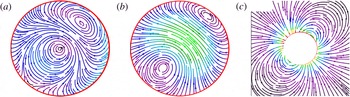
Figure 1 shows an illustrative example of a chiral self-propelling droplet with an
 $\ell =1$
component of body force density given by (here
 $a=1$
)
 $$\begin{eqnarray}\boldsymbol{f}^{\ell =1}=\mathop{\sum }_{m}\unicode[STIX]{x1D6FC}_{m}r(Y_{1m}\boldsymbol{e}_{r}-\unicode[STIX]{x1D6FB}_{s}Y_{1m}/2)+\unicode[STIX]{x1D6FE}_{m}(5r-6r^{2})\boldsymbol{e}_{r}\times \unicode[STIX]{x1D735}_{s}Y_{1m}.\end{eqnarray}$$
Coefficients are chosen such that both the total force and the total torque generated by this density vanish. In figure 1, the flow lines of the force density
 $\boldsymbol{f}$
and the flow fields
 $\boldsymbol{v}^{\pm }$
are shown in the
 $x{-}z$
plane. This simple example already shows that it is not straightforward to guess the internal flow field for a given force density field.
(a) Flow lines of the force density, and (b) internal and (c) external flow fields in the
 $xz$
plane with parameters
 $\unicode[STIX]{x1D6FC}_{0}=1$
,
 $\unicode[STIX]{x1D6FC}_{1}=-\unicode[STIX]{x1D6FC}_{-1}^{\ast }=1.7+0.5\,\text{i}$
,
 $\unicode[STIX]{x1D6FE}_{0}=1$
,
 $\unicode[STIX]{x1D6FE}_{1}=-\unicode[STIX]{x1D6FE}_{-1}^{\ast }=1.2+1.7\,\text{i}$
. It should be noted that it is not straightforward to guess the internal flow from the force field and the external flow. Magnitudes of vectors are coded in spectral sequence (black–violet–blue–green–yellow–red) online.

4.3 Conclusions: active body forces
In this section, we have related the linear and rotational motion of the droplet to the vector multipole moments of a given field of active body force densities and calculated the corresponding internal and external flow. Force-free translational motion can be achieved by a general power law dependence of the force density,
 $\boldsymbol{f}^{\,act}=(r/a)^{\unicode[STIX]{x1D708}}\boldsymbol{f}_{\unicode[STIX]{x1D708}}$
, such that forces are balanced in each radial shell inside the droplet. The translational velocity of the droplet is determined by the amplitude and power
 $\unicode[STIX]{x1D708}$
of the force as well as the two viscosities of the inside and outside fluid. Torque-free rotational motion requires at least two different power laws for the force density and cannot be fulfilled for each radial shell separately. The rotational flow inside the droplet depends in a non-trivial way on the assumed force density, whereas the rotational flow outside vanishes, as for a squirmer (Pak & Lauga Reference Pak and Lauga2014). Consequently, the rotational velocity of the droplet is a function of the interior viscosity only.
5 Active stresses
To make contact with continuum descriptions of active matter inside a droplet or cell, let us consider an active stress tensor with Cartesian components
 $$\begin{eqnarray}\unicode[STIX]{x1D70E}_{ij}^{act}=\left(p_{i}(\boldsymbol{r})p_{j}(\boldsymbol{r})-{\textstyle \frac{1}{3}}p^{2}(\boldsymbol{r})\unicode[STIX]{x1D6FF}_{ij}\right).\end{eqnarray}$$
This stress tensor originates from an active polar medium described by the polarisation field
 $\boldsymbol{p}(\boldsymbol{r})$
. Its origin is discussed in detail in Kruse et al. (Reference Kruse, Joanny, Jülicher, Prost and Sekimoto2004) and Joanny et al. (Reference Joanny, Jülicher, Kruse and Prost2007). Such active stresses generate a viscous flow inside the cell or droplet, which in turn gives rise to self-propulsion.
We restrict the discussion to the simple case of a director field, which only contains
 $\ell =0$
and
 $\ell =1$
,
 $m=0$
modes, i.e. it can be written in the form
 $$\begin{eqnarray}\boldsymbol{p}(r,\unicode[STIX]{x1D703},\unicode[STIX]{x1D711})=(p_{1}(r)\cos \unicode[STIX]{x1D703}+p_{0}(r))\boldsymbol{e}_{r}-p_{2}(r)\sin \unicode[STIX]{x1D703}\boldsymbol{e}_{\unicode[STIX]{x1D703}}.\end{eqnarray}$$
To determine the interior flow, we first compute the body force density
 $\boldsymbol{f}=-(\unicode[STIX]{x1D735}\boldsymbol{\cdot }\boldsymbol{p})\boldsymbol{p}-(\,\boldsymbol{p}\boldsymbol{\cdot }\unicode[STIX]{x1D735})\boldsymbol{p}+(1/3)\unicode[STIX]{x1D735}\boldsymbol{p}^{2}$
, with the explicit result given in appendix A.3. (If we start from an expansion of a general
 $\boldsymbol{p}(\boldsymbol{r})$
into vector spherical harmonics, the expansion of the terms quadratic in
 $\boldsymbol{p}$
, which determine
 $\boldsymbol{f}$
, can be performed straightforwardly by standard methods (Edmonds Reference Edmonds1957), but it is tedious and the result is not very illuminating. It has been worked out in detail in Moses (Reference Moses1974).) The polarisation of (5.2) gives rise to force components with
 $\ell =0,1,2$
. The
 $\ell =0$
component can be absorbed into the inhomogeneous pressure (see (4.4)) and contributes to the balance of uniform outside and inside pressure by the uniform surface tension. The
 $\ell =1$
modes from (A 41),
 $$\begin{eqnarray}\displaystyle \left.\begin{array}{@{}c@{}}\displaystyle f_{r}^{(1)}=-\frac{4}{3}(p_{0}p_{1})^{\prime }-\frac{4}{r}p_{0}p_{1}+\frac{2}{r}p_{0}p_{2},\\ \displaystyle f_{\unicode[STIX]{x1D703}}^{(1)}=(p_{0}p_{2})^{\prime }+\frac{3}{r}p_{0}p_{2}-\frac{2}{3r}p_{1}p_{0},\end{array}\right\} & & \displaystyle\end{eqnarray}$$
with
 $p_{i}^{\prime }=\text{d}p_{i}/\text{d}r$
, generate translational and rotational motion of the droplet. We will comment on the
 $\ell =2$
component below.
Without further assumptions on
 $\boldsymbol{p}(\boldsymbol{r})$
, the stress tensor is discontinuous across the interface and we have both active body forces and active tractions, so that the condition of vanishing total force reads
 $$\begin{eqnarray}\int _{V}\,\text{d}V\boldsymbol{f}^{\,act}(r)-\int _{\unicode[STIX]{x2202}V}\,\text{d}^{2}S\unicode[STIX]{x1D748}^{act}\boldsymbol{n}=0.\end{eqnarray}$$
With the ansatz of (5.2), force balance can be checked explicitly by computing the two terms separately,
 $$\begin{eqnarray}\int _{V}\,\text{d}V\boldsymbol{f}^{\,act}(r)=-\frac{8\unicode[STIX]{x03C0}}{3}a^{2}p_{0}(a)(\!2p_{1}(a)/3+p_{2}(a))\boldsymbol{e}_{z}=\int _{\unicode[STIX]{x2202}V}\,\text{d}^{2}S\,\unicode[STIX]{x1D748}^{act}\boldsymbol{n}.\end{eqnarray}$$
A simple example for the polarisation that vanishes on the surface of the droplet is
 $p_{i}(r)=p_{i}r/a(1-r/a)$
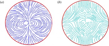
, implying the vanishing of the stress tensor on the surface of the droplet and hence the absence of tractions. The order parameter field and the corresponding force densities are shown for this example in figure 2.
Flow lines in the
 $xz$
plane of (a) the polar order parameter (according to (5.2)) and (b) the force density (according to (A 40)), with parameters
 $p_{0}=0.2$
,
 $p_{1}=p_{2}=1$
. The order parameter field is a simple dipole (
 $\ell =0$
and
 $\ell =1$
modes), but the force density field also contains
 $\ell =2$
modes and therefore looks qualitatively different.

The external flow field is easily computed from the general formalism in § 4.1. The details of the calculation are given in appendix A.3. The centre of mass velocity of the droplet is determined by the viscosities of the inside and outside fluid,
 $\unicode[STIX]{x1D702}^{\pm }$
, and by the coefficients of the polarisation,
 $p_{0}$
,
 $p_{1}$
,
 $p_{2}$
, according to
 $$\begin{eqnarray}\boldsymbol{v}_{CM}=\sqrt{\frac{3}{2\unicode[STIX]{x03C0}}}\frac{ap_{0}}{3(2\unicode[STIX]{x1D706}+3)}\left\{\frac{7p_{1}+p_{2}}{210\unicode[STIX]{x1D702}^{-}}-\frac{2p_{1}+11p_{2}}{60\unicode[STIX]{x1D702}^{+}}\right\}\boldsymbol{e}_{z}.\end{eqnarray}$$
Depending on the physical properties of the active matter and the interface, the director field has to fulfil boundary conditions. We mention two possibilities of strong anchoring. First, the director field may be aligned with the surface, implying
 $p_{0}(a)=p_{1}(a)=0$
. Second, the director field may be oriented perpendicular to the surface, implying
 $p_{2}(a)=0$
. In the first case, the tractions vanish, whereas in the second case, we have both active tractions and active body forces. The computation for the general case with both non-zero body forces and non-zero tractions is cumbersome but straightforward. Since we are dealing with linear equations, the flow fields due to tractions, as discussed in § 3, and the flow fields due to body forces only, as discussed in § 4, can be superimposed.
Before closing this section, two remarks are in order. First, it should be noted that the
 $\ell =1$
components of the force density are all proportional to
 $p_{0}$
; i.e. a director field, which only possesses
 $\ell =1$
,
 $m=0$
components, like for example
 $\boldsymbol{p}\propto \boldsymbol{e}_{z}$
, will not lead to self-propulsion. Finally, we note that even our simple ansatz for
 $\boldsymbol{p}(\boldsymbol{r})$
in general gives rise to a force density with
 $\ell =2$
. (For the explicit expression, see (A 41) in appendix A.3.) Although these higher modes can be neglected, if one calculates the droplet velocities at a fixed time, they will in general cause deformations of the droplet away from its spherical shape. Physically, these deformations are controlled by the surface tension, so that it is possible to describe weakly deformed droplets in a perturbation expansion in
 $1/\unicode[STIX]{x1D6FE}_{0}$
. It should be noted that only those higher-
 $\ell$
modes that produce a surface velocity
 $\propto \boldsymbol{e}_{r}$
will deform the droplet.
6 Droplet trajectories
6.1 Rigid active matter and droplet velocities
In the previous sections, we have calculated the flow fields of a droplet in the LF at a single fixed time. Now, we want to construct time-dependent flows of the fluids and trajectories of the droplet as a continuum of such single time snapshots. A necessary condition for the validity of this quasisteady-state approximation is that – in the limit of small Reynolds number
 $Re$
– the product of Reynolds and Strouhal numbers is also small, i.e.
 $Re\cdot S=\unicode[STIX]{x1D6FA}L^{2}/\unicode[STIX]{x1D702}^{-}\ll 1$
(Kim & Karrila Reference Kim and Karrila2005). Here,
 $\unicode[STIX]{x1D6FA}^{-1}$
is a characteristic time scale for changes of the force density and
 $L$
is a characteristic length scale, which, for internal flow, should be smaller than
 $a$
. A typical time scale for dissipative momentum transport over
 $a=1~\unicode[STIX]{x03BC}\text{m}$
in aqueous solution (
 $\unicode[STIX]{x1D702}=10^{-6}~\text{m}~\text{s}^{-2}$
) is
 $a^{2}/\unicode[STIX]{x1D702}=10^{-6}~\text{s}$
, so that the quasi-static approximation should be valid for
 $\unicode[STIX]{x1D6FA}\ll 10^{6}$
Hz if the viscosity contrast
 $\unicode[STIX]{x1D706}=\unicode[STIX]{x1D702}^{-}/\unicode[STIX]{x1D702}^{+}$
stays
 $O(1)$
. Even if this condition is met, the induced acceleration of the droplet may lead to additional forces, which may change the trajectories. These forces were first found by Stokes (Reference Stokes1851), Boussinesq (Reference Boussinesq1885) and Basset (Reference Basset1888). We will postpone a study of these effects to future work and neglect them in the following. A critical study of the validity of this assumption for passive particles can be found in Feng & Joseph (Reference Feng and Joseph1995).
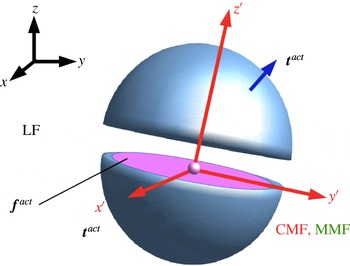
The time dependences of active force densities and tractions in the LF have not yet been specified. These densities are generated by active material, which shares the droplet interior with the Newtonian fluid, and which follows its own evolution equations. The material in the interior of micro-organisms has been modelled in many ways, for example as mixtures of simple (Dembo & Harlow Reference Dembo and Harlow1986) and complex (Kruse et al. Reference Kruse, Joanny, Jülicher, Prost and Sekimoto2005; Joanny et al. Reference Joanny, Jülicher, Kruse and Prost2007) active and passive fluids, or as a biphasic poro-elastic medium (Biot Reference Biot1955; deGennes Reference deGennes1976; Moeendarbary et al. Reference Moeendarbary, Valon, Fritzsche, Harris, Moulding, Thrasher, Stride, Mahadevan and Charras2013) with a distribution of active force densities or stress tensors, produced by molecular motors and (dis)-assembly of semi-flexible polymers (Loisel et al. Reference Loisel, Boujemaa, Pantaloni and Carlier1999). In all cases, the resulting evolution equations are quite complex. In the present subsection, we discuss a model of rigid active matter, which consists of a sparse rigid statistically isotropic structure, which carries the active forces and is immersed in a Newtonian fluid. This model, although highly simplified, is not unreasonable as an approximate continuum description on time scales that do not exceed the reorganisation time of the cytoskeleton. Its main advantage is that it allows for simple closed equations of motion of the droplet. A schematic view of our model is shown in figure 3.
Schematic view of our model and the frames of reference used in the main text. The droplet is cut open to show its interior. Inside and outside flow is created by active force densities
 $\boldsymbol{f}^{\,act}(\boldsymbol{r},t)$
in the interior and/or by active tractions
 $\boldsymbol{t}^{\,act}(\boldsymbol{r},t)$
in the interface. The droplet interior contains a sparse rigid statistically isotropic structure, with its centre fixed to the centre of the droplet. It carries the active elements, which produce
 $\boldsymbol{f}^{\,act}$
and
 $\boldsymbol{t}^{\,act}$
, and it still can rotate relative to the interior fluid. The motion of the droplet is observed from the LF. The co-moving frame (CMF) is fixed to the rigid structure and the momentary material frame (MMF) is an LF, which coincides with CMF at one instant of time. Calculations of flow fields and translational and rotational velocities of the droplet have been performed in the MMF, and thus the polar axis of the spherical coordinates is the
 $z^{\prime }$
axis.

As in every continuum description, let us label an element of the active material by
 $X$
. At an initial time
 $t=0$
, we assume that the element is at rest in the LF at position
 $\boldsymbol{X}_{0}$
in a quiet fluid, and in the course of time it follows a trajectory
 $\boldsymbol{X}(t)=\boldsymbol{X}(\boldsymbol{X}_{0},t)$
with velocity
 $\boldsymbol{v}_{m}(X,t)=\text{d}\boldsymbol{X}(t)/\text{d}t$
. If, for example, the material elements do not interact and move convectively in the Newtonian fluid, the material velocity equals the fluid velocity
 $\boldsymbol{v}_{m}(X,t)=\boldsymbol{v}^{-}(\boldsymbol{X}(t),t)$
. In the following we will restrict the discussion to a particularly simple case. We suppose that the active material is tied to parts of a polymeric (cyto)-skeleton, which can be modelled as a rigid structure. Thus, it can only undergo rigid body motions, composed of rotations
 $\hat{\boldsymbol{R}}(t)$
with respect to some material point and translations
 $\boldsymbol{b}(t)$
, i.e.
 $\boldsymbol{X}(t)=\hat{\boldsymbol{R}}(t)\boldsymbol{X}(0)+\boldsymbol{b}(t)$
, and thus the corresponding material velocities are given by
 $\boldsymbol{v}_{m}(\boldsymbol{X},t)=\boldsymbol{v}_{0}+\unicode[STIX]{x1D74E}_{m}(t)\times [\boldsymbol{X}(t)-\boldsymbol{b}(t)]$
, with
 $\boldsymbol{v}_{0}=\text{d}\boldsymbol{b}/\text{d}t$
.
As an additional constraint, we require that the translational motion of the skeleton and the translational motion of the droplet coincide, i.e.
 $\boldsymbol{v}_{0}=\boldsymbol{v}_{CM}$
. This constraint can be realised in various ways, for example by anchoring at least four material points of the skeleton (not all in the same plane) within the interface. This fixes the centre of the sphere rigidly to the skeleton, reminiscent of the anchoring at the microtubule-organising centre. The motion of the skeleton is thus restricted to rotations within the droplet. Without such a constraint, the skeleton could perform translational motions relative to the centre of the sphere – like, for example, an active particle propelling in the interior of the droplet – which we do not want to discuss here.
In the following, we will refer to
 $\unicode[STIX]{x1D74E}_{m}$
as the angular velocity of the skeleton. To compute this angular velocity from the flow field
 $\boldsymbol{v}^{-}$
, we consider the dissipative forces exerted by the flow on the skeleton in the MMF as proportional to the relative velocity between skeleton and fluid, i.e. proportional to
 $\int _{K}\unicode[STIX]{x1D70C}_{p}(\boldsymbol{v}_{m}-\boldsymbol{v}^{-})\,\text{d}V$
. A part of these forces is compensated by the rigid constraints; the other part is the only remaining force on the skeleton, which thus has to vanish. A convenient way to calculate the uncompensated generalised force on the rigid skeleton is to start from the dissipation function (Landau & Lifshitz Reference Landau and Lifshitz1976)
 $D(\unicode[STIX]{x1D74E}_{m})=(\unicode[STIX]{x1D705}/2)\int _{K}\unicode[STIX]{x1D70C}_{p}(\boldsymbol{r})(\boldsymbol{v}^{m}(\boldsymbol{r})-\boldsymbol{v}^{-}(\boldsymbol{r}))^{2}\,\text{d}V$
. The friction coefficient
 $\unicode[STIX]{x1D705}>0$
is unimportant in the following. The derivative of
 $D$
with respect to
 $\unicode[STIX]{x1D74E}_{m}$
is the generalised force, which has to vanish. The resulting relation
 $\int _{K}[\boldsymbol{r}\times (\boldsymbol{v}_{CM}+\unicode[STIX]{x1D74E}_{m}\times \boldsymbol{r}-\boldsymbol{v}^{-})]\unicode[STIX]{x1D70C}_{p}\,\text{d}V=0$
can be written in the form
 $$\begin{eqnarray}\mathop{\sum }_{j=1}^{3}\boldsymbol{I}_{ij}(\unicode[STIX]{x1D714}_{m})_{j}=\int _{K}[\unicode[STIX]{x1D70C}_{p}(\boldsymbol{r})\boldsymbol{r}\times (\boldsymbol{v}^{-}(\boldsymbol{r})-\boldsymbol{v}_{CM})]_{i}\,\text{d}V.\end{eqnarray}$$
Here,
 $\boldsymbol{I}_{ij}=\int \unicode[STIX]{x1D70C}_{p}(r^{2}\unicode[STIX]{x1D6FF}_{ij}-x_{i}x_{j})$
. It should be noted that
 $\unicode[STIX]{x1D74E}_{m}$
depends on the structure of the skeleton and in general differs from the angular velocity
 $\unicode[STIX]{x1D74E}$
defined in (2.7). If the skeleton density is spherically symmetric,
 $\boldsymbol{I}_{ij}=I\unicode[STIX]{x1D6FF}_{ij}$
, with
 $I=(8\unicode[STIX]{x03C0}/3)\int _{0}^{a}\unicode[STIX]{x1D70C}_{p}(r)r^{4}$
, we obtain
 $$\begin{eqnarray}\unicode[STIX]{x1D74E}_{m}=\frac{1}{I}\int _{K}\unicode[STIX]{x1D70C}_{p}(r)\boldsymbol{r}\times \boldsymbol{v}^{-}\,\text{d}V.\end{eqnarray}$$
For a homogeneous
 $\unicode[STIX]{x1D70C}_{p}(r)=\unicode[STIX]{x1D70C}_{p}$
, the constant
 $I$
becomes
 $I=(8\unicode[STIX]{x03C0}a^{5}/15)\unicode[STIX]{x1D70C}_{p}$
. In this case,
 $\unicode[STIX]{x1D74E}_{m}$
coincides with
 $\unicode[STIX]{x1D74E}$
from (2.7).
For other structures, there will be a relative rotational motion of the skeleton and the internal fluid. If, for example, the skeleton mass is essentially concentrated in a spherical nucleus with radius
 $a_{nuc}<a$
, the motion is reminiscent of the observed rotation of a cell nucleus in the interior of a cell (Kumar et al.
Reference Kumar, Maitra, Sumit, Ramaswamy and Shivashankar2014). On the other hand, if the skeleton were concentrated in a thin shell at the interface, i.e.
 $\unicode[STIX]{x1D70C}_{p}(r)=\unicode[STIX]{x1D70C}_{p}\unicode[STIX]{x1D6FF}(r-a)$
, then
 $I=(8\unicode[STIX]{x03C0}a^{4}/3)\unicode[STIX]{x1D70C}_{p}$
, and the rigid shell would rotate relative to the internal fluid.
Three frames of reference, which are used in the following, are defined with respect to the skeleton (see figure 3). At time
 $t=0$
, when each
 $X$
is placed at its corresponding
 $\boldsymbol{X}_{0}$
, we choose a Cartesian system, with its origin at the centre of the sphere,
 $\boldsymbol{r}_{CM}$
, and unit vectors
 $\boldsymbol{e}_{\unicode[STIX]{x1D6FC}}$
,
 $\unicode[STIX]{x1D6FC}=1,2,3$
. This is our LF. The frame at any other time, with its origin at
 $\boldsymbol{X}(\boldsymbol{X}_{0}=\mathbf{0},t)$
and rotated unit vectors
 $\hat{\boldsymbol{R}}(t)\boldsymbol{e}_{\unicode[STIX]{x1D6FC}}$
, is called the CMF. At
 $t=0$
, the CMF and the LF coincide, i.e.
 $\hat{\boldsymbol{R}}(0)=\hat{\mathbf{1}}$
and
 $\boldsymbol{b}(0)=\mathbf{0}$
. Per definition, the skeleton is at rest in the CMF. Its density
 $\unicode[STIX]{x1D70C}_{p}(X)$
carries the active force density
 $\boldsymbol{f}^{\,act}(X,t)$
, which may depend upon time. Another LF, with origin and axes coinciding with those of the CMF at a fixed instant
 $t$
will be called the MMF in the following. The calculations of §§ 3–5 have been performed in this frame.
The active matter in the droplet interior will in general also modify the internal flow field. For a droplet filled with a rigid gel and a viscous fluid, there is an additional permeation force (Milner Reference Milner1993; Callan & Jülicher Reference Callan and Jülicher2011), which enters the force balance. This leads to a modified Stokes equation of the form
 $\unicode[STIX]{x1D735}\boldsymbol{\cdot }\unicode[STIX]{x1D748}^{-}=\unicode[STIX]{x1D735}p-\unicode[STIX]{x1D701}(\unicode[STIX]{x1D70C}_{p})(\boldsymbol{v}-\boldsymbol{v}^{m})-\boldsymbol{f}^{\,act}-\boldsymbol{f}^{ext}$
. Here,
 $\unicode[STIX]{x1D701}(\unicode[STIX]{x1D70C}_{p})$
is a permeation coefficient, which depends upon the detailed structure of the gel. In the following, we will assume that the gel fraction is small, and
 $\unicode[STIX]{x1D701}$
, which vanishes with
 $\unicode[STIX]{x1D70C}_{P}$
, is so small that we can neglect the permeation force. Then,
 $\boldsymbol{v}^{-}$
is entirely due to the active and external force densities, and can be calculated using (2.1).
The time dependence of the force density
 $\boldsymbol{f}^{\,act}(\boldsymbol{r},t)$
and the skeleton density
 $\unicode[STIX]{x1D70C}_{p}(\boldsymbol{r},t)$
produced by active material at position
 $\boldsymbol{r}$
in the LF are now easily obtained. In the CMF, the position and orientation of each material element are time-independent, and only the explicit time dependence of the force density remains, i.e.
 $\unicode[STIX]{x1D70C}_{p}(\boldsymbol{r},t)=\unicode[STIX]{x1D70C}_{p}(\boldsymbol{X}_{0}=\boldsymbol{r})$
and
 $\boldsymbol{f}^{\,act}(\boldsymbol{r},t)=\boldsymbol{f}^{\,act}(\boldsymbol{X}_{0}=\boldsymbol{r},t)$
. In the LF, these quantities are co-translated and co-rotated along the trajectory of the active material element, so that
 $$\begin{eqnarray}\frac{\text{d}f_{i}^{act}(\boldsymbol{r},t)}{\text{d}t}=(\boldsymbol{v}_{CM}+\unicode[STIX]{x1D74E}_{m}\times \boldsymbol{r})\boldsymbol{\cdot }\unicode[STIX]{x1D735}\boldsymbol{f}_{i}^{\,act}(\boldsymbol{r},t)+\frac{\unicode[STIX]{x2202}f_{i}^{act}}{\unicode[STIX]{x2202}t},\end{eqnarray}$$
and correspondingly
 $\text{d}\unicode[STIX]{x1D70C}_{p}(\boldsymbol{r},t)/\text{d}t=(\boldsymbol{v}_{CM}+\unicode[STIX]{x1D74E}_{m}\times \boldsymbol{r})\boldsymbol{\cdot }\unicode[STIX]{x1D735}\unicode[STIX]{x1D70C}_{p}(t)$
.
6.2 Trajectories
To determine the trajectories of the droplet in the LF, we can use (2.6) and (6.1), (6.2). Due to our assumption that the active material is tied to the skeleton, the dynamics of this skeleton in the LF is fully characterised by the transformation of the MMF, spanned by coordinate unit vectors
 $\boldsymbol{e}_{i}$
,
 $i=1,2,3$
, and rooted at the centre of the sphere,
 $\boldsymbol{r}_{CM}(t)$
, into the Cartesian LF spanned by
 $\boldsymbol{a}_{i}$
,
 $i=1,2,3$
. The equations of motion for the droplet skeleton thus become those of a rigid body,
 $$\begin{eqnarray}\displaystyle & \displaystyle \frac{\text{d}\boldsymbol{r}_{CM}}{\text{d}t}=\mathop{\sum }_{i=1}^{3}v_{CM,i}(t)\boldsymbol{e}_{i}(t), & \displaystyle\end{eqnarray}$$
 $$\begin{eqnarray}\displaystyle & \displaystyle \frac{\text{d}\boldsymbol{e}_{i}}{\text{d}t}=\unicode[STIX]{x1D74E}_{m}(t)\times \boldsymbol{e}_{i}(t), & \displaystyle\end{eqnarray}$$
with translational and rotational velocities, which are linearly related to the multipole moments of the internal force distributions via the flow fields
 $\boldsymbol{v}^{\pm }$
. In the previous sections, we have calculated these relations explicitly. In this section, we discuss how features of the trajectories are linked to features of the body force distributions of self-propelled motion by considering a few illustrating cases. We restrict the examples to a droplet with a homogeneous skeleton, i.e.
 $\unicode[STIX]{x1D74E}_{m}=\unicode[STIX]{x1D74E}$
, and choose a radius
 $a=1~\unicode[STIX]{x03BC}\text{m}$
to produce representative numerical values, for which we measure lengths in
 $\unicode[STIX]{x03BC}\text{m}$
, time in s and forces in pN.
Force multipoles and velocities are related by (4.7), (4.11), which can be written in the form
 $$\begin{eqnarray}\sqrt{2}v_{CM,z}=v_{CM,0}=\unicode[STIX]{x1D6FC}_{0}/C,\quad -v_{CM,x}+\text{i}v_{CM,y}=v_{CM,1}=\unicode[STIX]{x1D6FC}_{1}/C\end{eqnarray}$$
and
 $$\begin{eqnarray}\sqrt{2}\unicode[STIX]{x1D714}_{z}=\unicode[STIX]{x1D714}_{0}=\tilde{\unicode[STIX]{x1D6FE}}_{0}/D,\quad -\unicode[STIX]{x1D714}_{x}+\text{i}\unicode[STIX]{x1D714}_{y}=\unicode[STIX]{x1D714}_{1}=\tilde{\unicode[STIX]{x1D6FE}_{1}}/D,\end{eqnarray}$$
with
 $C=\sqrt{(2\unicode[STIX]{x03C0}/3)}3(\unicode[STIX]{x1D708}+5)(2+3\unicode[STIX]{x1D706})(\unicode[STIX]{x1D702}^{+}/a^{2})$
and
 $D=\sqrt{(2\unicode[STIX]{x03C0}/3)}(\unicode[STIX]{x1D702}^{-}/ac_{\unicode[STIX]{x1D6FE}})$
. For our illustrations, we choose
 $\unicode[STIX]{x1D706}=5$
and
 $\unicode[STIX]{x1D708}=1$
in
 $C$
and
 $\unicode[STIX]{x1D708}_{1}=1$
and
 $\unicode[STIX]{x1D708}_{2}=2$
(see (4.11)) in
 $c_{\unicode[STIX]{x1D6FE}}$
. Then, the constant
 $C=c_{v}\times 10^{9}~\text{s}^{-1}\approx 0.44\times 10^{9}~\text{s}^{-1}$
and
 $D=c_{\unicode[STIX]{x1D714}}\times 10^{9}~\unicode[STIX]{x03BC}\text{m}~\text{s}^{-1}\approx 0.41\times 10^{9}~\unicode[STIX]{x03BC}\text{m}~\text{s}^{-1}$
.
The force
 $\boldsymbol{f}^{\,act}$
and the corresponding multipole moments
 $\unicode[STIX]{x1D6FC}_{m}$
,
 $\unicode[STIX]{x1D6FE}_{m}$
are force densities per mass density with units
 $\unicode[STIX]{x03BC}\text{m}~\text{s}^{-2}$
. We prefer to relate velocities to force densities
 $\unicode[STIX]{x1D746}_{f}$
per volume, with corresponding multipoles
 $\widehat{\unicode[STIX]{x1D6FC}}_{m}$
,
 $\widehat{\unicode[STIX]{x1D6FE}}_{m}$
given in
 $\text{pN}~\unicode[STIX]{x03BC}\text{m}^{-3}=10^{-12}~\text{N}~\unicode[STIX]{x03BC}\text{m}^{-3}$
, to facilitate the comparison with forces generated by molecular mechanisms. For aqueous solutions, the volume force density is related to
 $\boldsymbol{f}^{\,act}$
by
 $\boldsymbol{f}^{\,act}[\unicode[STIX]{x03BC}\text{m}~\text{s}^{-2}]=\unicode[STIX]{x1D746}_{f}/\unicode[STIX]{x1D70C}_{0}=10^{9}\unicode[STIX]{x1D746}_{f}[\text{pN}~\unicode[STIX]{x03BC}\text{m}^{-3}]$
, so that
 $$\begin{eqnarray}\displaystyle \left.\begin{array}{@{}c@{}}\displaystyle v_{a}[\unicode[STIX]{x03BC}\text{m}~\text{s}^{-1}]=\widehat{\unicode[STIX]{x1D6FC}}_{a}/c_{v}[\text{pN}~\unicode[STIX]{x03BC}\text{m}^{-3}]\approx 2.27\times \widehat{\unicode[STIX]{x1D6FC}}_{a}[\text{pN}~\unicode[STIX]{x03BC}\text{m}^{-3}],\quad a=0,1,\\ \displaystyle \unicode[STIX]{x1D714}_{a}[1~\text{s}^{-1}]=\widehat{\unicode[STIX]{x1D6FE}}_{a}/c_{\unicode[STIX]{x1D714}}[\text{pN}~\unicode[STIX]{x03BC}\text{m}^{-3}]\approx 2.44\times \widehat{\unicode[STIX]{x1D6FE}}_{a}[\text{pN}~\unicode[STIX]{x03BC}\text{m}^{-3}],\quad a=0,1.\end{array}\right\} & & \displaystyle\end{eqnarray}$$
When comparing with molecular mechanisms of force generation, one should remember that
 $\widehat{\unicode[STIX]{x1D6FC}}_{a}$
and
 $\widehat{\unicode[STIX]{x1D6FE}}_{a}$
only contain the
 $\ell =1$
part of the total force density.
Figures 4–7 depict trajectories of the centre of mass (scales in
 $\unicode[STIX]{x03BC}\text{m}$
) in (a) and illustrate the rotational motion in (b). For the latter, we follow a marked point on the interface in time. This point has position vector
 $\boldsymbol{y}(t)$
in the LF and develops in time according to
 $\boldsymbol{y}(t)=\hat{\boldsymbol{R}}(t)\boldsymbol{y}(0)+\boldsymbol{r}_{CM}(t)$
. We plot
 $\unicode[STIX]{x0394}\boldsymbol{y}(t)=\boldsymbol{y}(t)-\boldsymbol{r}_{CM}(t)=\hat{\boldsymbol{R}}(t)\boldsymbol{y}(0)=\sum _{i}b_{i}\boldsymbol{e}_{i}(t)$
and have chosen
 $b_{i}=1$
,
 $i=1,2,3$
.
Case 1. For the simple case of force densities, which are time-independent in the CMF, the resulting trajectories from (6.4), (6.5) are helices, as shown in figure 4. The axis of the helix is parallel to
 $\unicode[STIX]{x1D74E}$
, which we have chosen to be the
 $z$
-axis. If the chiral parts of the force densities vanish (i.e.
 $\unicode[STIX]{x1D6FE}_{m}=0$
), the trajectories become straight lines.
For time-independent force densities, the trajectories are helices (or straight lines, if
 $\unicode[STIX]{x1D74E}=0$
). The example shows a trajectory generated by force density multipoles
 $\widehat{\unicode[STIX]{x1D6FE}_{0}}=10\,\sqrt{2}c_{\unicode[STIX]{x1D714}}$
,
 $\tilde{\unicode[STIX]{x1D6FE}}_{1}=0$
and
 $\widehat{\unicode[STIX]{x1D6FC}}_{0}=10\,\sqrt{2}c_{v}$
,
 $\widehat{\unicode[STIX]{x1D6FC}}_{1}=c_{v}(-3+2\,\text{i})$
, given in
 $[\text{pN}~\unicode[STIX]{x03BC}\text{m}^{-3}]$
. Panel (a) depicts
 $\boldsymbol{r}_{CM}(t)$
and panel (b) shows the rotational motion of
 $\unicode[STIX]{x0394}\boldsymbol{y}(t)$
, as defined in the main text.

Case 2. Force densities, which oscillate with a single frequency and vanish when averaged over a period, can create unbounded translational motion, as shown in figure 5. The unbounded translation requires non-vanishing chiral components of the force densities.
Periodic force densities with vanishing averages over one period may nevertheless lead to unbounded translations. Panel (a) shows the trajectory of
 $\boldsymbol{r}_{CM}$
and panel (b) depicts the rotational motion of
 $\unicode[STIX]{x0394}\boldsymbol{y}(t)$
(see the main text) for force multipoles (in
 $[\text{pN}~\unicode[STIX]{x03BC}\text{m}^{-3}]$
)
 $\widehat{\unicode[STIX]{x1D6FE}}_{0}=0.1\,\sqrt{2}\,c_{\unicode[STIX]{x1D714}}\sin (t)$
and
 $\widehat{\unicode[STIX]{x1D6FE}}_{1}=0$
,
 $\widehat{\unicode[STIX]{x1D6FC}}_{0}=0$
,
 $\widehat{\unicode[STIX]{x1D6FC}}_{1}=0.1\,c_{v}(-\text{sin}(t)+\text{i}\cos (t))$
.

Case 3. On the other hand, it is also possible to get helical motion without any chiral components of the forces. In figure 6(a), the chiral components and thus the angular velocity
 $\unicode[STIX]{x1D74E}$
vanish. The force density oscillates with a single frequency but has a non-vanishing average over one period. If a constant chiral force density is added to the oscillating force, rosette-shaped trajectories appear, as shown in figure 6(b). These may also be superimposed with a translational motion.
(a) Helical motion arising from periodic non-chiral force densities, with multipoles (in
 $[\text{pN}~\unicode[STIX]{x03BC}\text{m}^{-3}]$
)
 $\widehat{\unicode[STIX]{x1D6FC}_{0}}=0$
and
 $\widehat{\unicode[STIX]{x1D6FC}_{1}}=c_{v}(-(0.1+0.6\cos (t))+\text{i}(0.1+0.6\sin (t)))$
. (b) A chiral force density with
 $\widehat{\unicode[STIX]{x1D6FE}}_{0}=0.2\,\sqrt{2}c_{\unicode[STIX]{x1D714}}$
,
 $\widehat{\unicode[STIX]{x1D6FE}}_{1}=0$
is added to the system of (a), resulting in rosette-shaped trajectories. The depicted rosette is simple and closed, because the ratio of the frequencies in
 $\boldsymbol{v}_{CM}$
(which is 1) and
 $\unicode[STIX]{x1D74E}$
is a rational number (
 $1/5$
).

Case 4. Finally, if the forces contain more than one frequency, the zoology of the trajectories gets more and more involved and will be discussed elsewhere. As an example, figure 7 shows the translational (figure 7 a) and rotational (figure 7 b) motion of a three-dimensional trajectory resulting from five different non-vanishing frequencies and a constant component of forces. Although this trajectory is smooth, it superficially resembles run-and-tumble type trajectories when observed from a fixed viewing angle.
This example shows a complex trajectory of
 $\boldsymbol{r}_{CM}$
and
 $\boldsymbol{b}$
(see the main text), resulting from a chiral force density
 $\widehat{\unicode[STIX]{x1D6FE}}_{0}=\sqrt{2}c_{\unicode[STIX]{x1D714}}[\text{pN}~\unicode[STIX]{x03BC}\text{m}^{-3}]$
,
 $\widehat{\unicode[STIX]{x1D6FE}}_{1}=c_{\unicode[STIX]{x1D714}}(-0.5\sin (t)+0.3\,\text{i}\,\sin (\sqrt{2}t))[\text{pN}~\unicode[STIX]{x03BC}\text{m}^{-3}]$
and
 $\widehat{\unicode[STIX]{x1D6FC}}_{0}=0.4\,\sqrt{2}c_{v}\sin (0.3t)[\text{pN}~\unicode[STIX]{x03BC}\text{m}^{-3}]$
,
 $\widehat{\unicode[STIX]{x1D6FE}}_{1}=c_{v}(-0.6\sin (1.9t)+0.8\,\text{i}\,\sin (1.1t))[\text{pN}~\unicode[STIX]{x03BC}\text{m}^{-3}]$
.

We have presented these few cases to illustrate that simple changes of the time dependences of active processes can lead to qualitatively different trajectories of self-propelled motion. Such changes in time dependences thus offer rich possibilities for steering self-propelled motion.
Simple models of self-propelled particles have been studied extensively over recent years, mainly to understand the collective behaviour of active matter. In these approaches, a swimmer is modelled as an anisotropic particle with constant linear and angular velocity, and is subject to noise due to the surrounding fluid. Here, we derive these velocities from the internal flow, generated by active structural elements within the swimmer. Constant velocities are shown to result from a time-independent forcing machinery, whereas oscillating forces give rise to time-dependent velocities and complex trajectories. The trajectories that we observe bear striking similarities with those of self-propelled particles (Bechinger et al. Reference Bechinger, Leonardo, Löwen, Reichhardt, Volpe and Volpe2016). In the latter case, complex behaviour results from the interplay of activity and (persistent) noise, whereas in our case, it is the result of the inherent machinery of a single swimmer. Important differences concern the small scales of the trajectories, which have features of a random walk for self-propelled particles, but are completely smooth in our case.
7 Conclusions and outlook
We have shown how spherical droplets of immiscible fluids can be propelled by activity mechanisms, which are based on active surface tractions
 $\boldsymbol{t}_{act}$
, active body force densities
 $\boldsymbol{f}_{act}$
, or both. In a first step, we have calculated the exact relations between vector multipole moments of active force densities or surface tractions, the flow fields, and the linear and angular momentum of the droplet.
In continuum models, active forces are described by active stress tensors inside the droplet. As an illustrating example, we considered an active polar medium, whose polarisation
 $\boldsymbol{p}$
generates active stresses of the form
 $\unicode[STIX]{x1D70E}_{ij}^{act}\sim p_{i}p_{j}-p^{2}\unicode[STIX]{x1D6FF}_{ij}/3$
. If stresses are discontinuous across the interface, they give rise to tractions localised at the interface, so that the general case comprises both tractions and body forces.
Energy is dissipated by the flow fields both inside and outside of the droplet, and we found that the ratio of dissipated energies in the outside and inside is universal, independent of the driving activity.
To compute the time-dependent flow fields and trajectories of the droplet, we need to specify the dynamics of the activity mechanism in a second step. We model this as being tied to a sparse rigid statistically isotropic skeleton, which is constrained to translate with the droplet.
We allow for an explicit time dependence of the activity mechanism in the co-moving frame, with a characteristic time scale
 $\unicode[STIX]{x1D6FA}^{-1}$
. In order to construct a droplet trajectory as a sequence of snapshots, which have been computed in the first step of our procedure, the inertial terms in the Navier–Stokes equation have to remain negligible. This is guaranteed if – besides the Reynolds number
 $Re$
– the product of the Reynolds number and the Strouhal number
 $S$
remains small. For micro-organisms, this criterion is fulfilled for
 $\unicode[STIX]{x1D6FA}\ll 10^{6}~\text{Hz}$
. For a droplet of radius
 $a=1~\unicode[STIX]{x03BC}\text{m}$
and typical values of material parameters, we find that velocities
 $\boldsymbol{v}_{CM}$
in
 $\unicode[STIX]{x03BC}\text{m}~\text{s}^{-1}$
and
 $\unicode[STIX]{x1D74E}$
in
 $1~\text{s}^{-1}$
are related to force densities in
 $\text{pN}~\unicode[STIX]{x03BC}\text{m}^{-3}$
by constants of order 1.
To exemplify the relations between the time dependence of body force densities and droplet trajectories, we considered four simple cases. (i) In the absence of an explicit time dependence of activity, the droplet trajectories are straight lines or helices, with in general non-collinear translational and rotational velocities. Specifically, the angular velocity vanishes for an autonomous swimmer, which is driven by active surface tractions and experiences no external torque. (ii) Force densities that oscillate with a single frequency and vanish when averaged over one period may create unbounded translational motion. (iii) Force densities that do not contain chiral components but oscillate with a single frequency may lead to helical trajectories. Additional chiral components may generate rosette-shaped trajectories. (iv) Forces oscillating with several incompatible frequencies may generate trajectories that resemble run-and-tumble type trajectories when observed from a constant viewing angle. These examples demonstrate that the time dependence of active forces is a very effective means to switch between qualitatively different types of motion.
Our approach can be extended in several ways. The simple droplet model can and should be improved in various ways to bring it closer to models of active micro-organisms. On the one hand, more details of force generating mechanisms can be included. For example, in Whitfield et al. (Reference Whitfield, Marenduzzo, Voituriez and Hawkins2014), the case of a two-dimensional droplet of active contractile fluid was studied. We are interested in three-dimensional biphasic droplets of active gels with a finite gel fraction and permeation force. Furthermore, the interface between the liquids should be replaced by a fluid or elastic membrane.
Another problem of interest is the motion of an active droplet in non-zero ambient flow, e.g. in channel flow or shear flow, which has been analysed in Tarama et al. (Reference Tarama, Menzel, ten Hagen, Wittkowski and Ohta2013) based on equations of motion derived from symmetry considerations. For ellipsoidal droplets and tangential stress boundary conditions, a numerical study was performed by Kanevsky, Shelley & Tornberg (Reference Kanevsky, Shelley and Tornberg2010). Zöttl & Stark (Reference Zöttl and Stark2013) studied an elongated active particle in Poiseuille flow. For droplets, the external flow might involve shape changes, which we have not considered so far, because we focused on the
 $l=1$
modes and the droplet motion. However, a perturbative analysis of shape changes for droplets with large surface tension should be possible following the method of Taylor (Reference Taylor1934) and Vlahoska, Blawzdziewicz & Loewenberg (Reference Vlahoska, Blawzdziewicz and Loewenberg2009).
The proposed formalism may also provide a starting point to discuss droplet motion in the presence of external forces, taxis or unsteady flow, including the changes in velocity. So far, we have only analysed the simplest case of a sedimenting active droplet, but it would be interesting to extend the analysis, taking into account the forces of Stokes (Reference Stokes1851), Boussinesq (Reference Boussinesq1885) and Basset (Reference Basset1888). For passive droplets, a corresponding equation of motion has been derived in Michaelidis & Feng (Reference Michaelidis and Feng1995), but for active droplets, we are not aware of any work in this direction.
Appendix A
A.1 General solution of the homogeneous Stokes equations in vector spherical harmonics
There are several ways to solve boundary value problems of the Stokes equations,
 $$\begin{eqnarray}\unicode[STIX]{x1D702}\unicode[STIX]{x1D6FB}^{2}\boldsymbol{v}=\unicode[STIX]{x1D735}p,\quad \unicode[STIX]{x1D735}\boldsymbol{\cdot }\boldsymbol{v}=0,\end{eqnarray}$$
with a spherical interface
 $\unicode[STIX]{x2202}K$
at
 $r=a$
. The general solution in spherical coordinates was first obtained by Lamb (Reference Lamb1879). Here, we use expansions in terms of scalar and vector spherical harmonics (VSHs), which we find particularly simple to match at spherical interfaces and convenient to reduce boundary value problems to linear equations. Alternatively, one may use Cartesian tensors (Ghose & Adhikari Reference Ghose and Adhikari2014; Einarsson & Mehlig Reference Einarsson and Mehlig2016) or spin-spherical harmonics (Newman & Penrose Reference Newman and Penrose1966).
Whereas scalar spherical harmonics
 $Y_{\ell m}$
are fairly standardised, there exist several versions of VSHs. We use
 $$\begin{eqnarray}\displaystyle & \displaystyle \boldsymbol{Y}_{\ell m0}=Y_{\ell m}\boldsymbol{e}_{r}, & \displaystyle\end{eqnarray}$$
 $$\begin{eqnarray}\displaystyle & \displaystyle \boldsymbol{Y}_{\ell m1}=\unicode[STIX]{x1D735}_{s}\boldsymbol{Y}_{\ell m}, & \displaystyle\end{eqnarray}$$
 $$\begin{eqnarray}\displaystyle & \displaystyle \boldsymbol{Y}_{\ell m2}=\boldsymbol{e}_{r}\times \unicode[STIX]{x1D735}_{s}\boldsymbol{Y}_{\ell m}. & \displaystyle\end{eqnarray}$$
These functions
 $\boldsymbol{Y}_{\ell ms}$
form a complete orthogonal set on the surface of a sphere with respect to the scalar product
 $(\,\boldsymbol{f},\boldsymbol{g})=\int _{-1}^{1}\,\text{d}(\cos \unicode[STIX]{x1D703})\int _{0}^{2\unicode[STIX]{x03C0}}\,\text{d}\unicode[STIX]{x1D711}\,\boldsymbol{f}^{\ast }(\unicode[STIX]{x1D703},\unicode[STIX]{x1D711})\boldsymbol{\cdot }\boldsymbol{g}(\unicode[STIX]{x1D703},\unicode[STIX]{x1D711})$
. The
 $s=0$
functions are normalised to 1, whereas the
 $s=1,2$
functions have norm
 $\sqrt{\ell (\ell +1)}$
.
Formulae for the elementary vector analytic operations (gradient, divergence and curl) acting on the
 $\boldsymbol{Y}_{\ell ms}$
can be found, for example, in Morse & Feshbach (Reference Morse and Feshbach1953). For the reader’s convenience, we include the representation of a gradient and a divergence, which will be used below. For
 $\unicode[STIX]{x1D735}p$
, one obtains
 $$\begin{eqnarray}\unicode[STIX]{x1D735}p(r,\unicode[STIX]{x1D703},\unicode[STIX]{x1D711})=\mathop{\sum }_{\ell ms}(\unicode[STIX]{x1D735}p)_{\ell ms}\boldsymbol{Y}_{\ell ms}=\mathop{\sum }_{\ell ,m}\frac{\text{d}p_{\ell m}}{\text{d}r}\boldsymbol{Y}_{\ell m0}+\frac{p_{\ell m}}{r}\boldsymbol{Y}_{\ell m1},\end{eqnarray}$$
where the sum runs over
 $\ell =0,1,2,\ldots$
and
 $m$
runs from
 $-\ell$
to
 $\ell$
in steps of width 1. The divergence takes on the form
 $$\begin{eqnarray}\unicode[STIX]{x1D735}\boldsymbol{\cdot }\boldsymbol{v}=\mathop{\sum }_{\ell m}(\unicode[STIX]{x1D735}\boldsymbol{\cdot }\boldsymbol{v})_{\ell m}Y_{\ell m}=\mathop{\sum }_{\ell ms}\left(\frac{\text{d}v_{\ell m0}}{\text{d}r}+\frac{2}{r}v_{\ell m0}-\frac{\ell (\ell +1)}{r}v_{\ell m1}\right)Y_{\ell m}.\end{eqnarray}$$
The incompressibility constraint implies two relations: first,
 $p$
obeys the Laplace equation
 $\unicode[STIX]{x1D6FB}^{2}p(r,\unicode[STIX]{x1D703},\unicode[STIX]{x1D711})=0$
, which is equivalent to
 $$\begin{eqnarray}\frac{\,\text{d}^{2}p_{\ell m}(r)}{\text{d}r^{2}}+\frac{2}{r}\frac{\text{d}p_{\ell m}}{\text{d}r}-\frac{\ell (\ell +1)}{r}p_{\ell m}=0\end{eqnarray}$$
for all possible
 $\ell$
and
 $m$
, and second, the expansion coefficients
 $v_{\ell m0}$
and
 $v_{\ell m1}$
are related by
 $$\begin{eqnarray}\frac{\text{d}v_{\ell m0}}{\text{d}r}+\frac{2}{r}v_{\ell m0}=\frac{\ell (\ell +1)}{r}v_{\ell m1}.\end{eqnarray}$$
The vector Laplace operator
 $\unicode[STIX]{x1D6FB}^{2}\boldsymbol{v}$
is diagonal in
 $\ell$
and
 $m$
, but for the VSH defined in (A 2) it is not diagonal in the index
 $s$
. It is easily checked by direct calculation that
 $\unicode[STIX]{x1D6FB}^{2}\boldsymbol{Y}_{\ell ms}=\sum _{s^{\prime }}h_{s^{\prime }s}^{t}\boldsymbol{Y}_{\ell \boldsymbol{m}\boldsymbol{s}^{\prime }}/r^{2}$
. The coefficients
 $h_{ss^{\prime }}^{t}=h_{s^{\prime }s}$
define a
 $3\times 3$
matrix
 $\hat{\unicode[STIX]{x1D65D}}$
, which is given by
 $$\begin{eqnarray}\hat{\unicode[STIX]{x1D65D}}=\left(\begin{array}{@{}ccc@{}}-[2+\ell (\ell +1)] & 2\ell (\ell +1) & 0\\ 2 & -\ell (\ell +1) & 0\\ 0 & 0 & -\ell (\ell +1)\end{array}\right),\end{eqnarray}$$
and which may be used to write the vector Laplace operator in the form
 $$\begin{eqnarray}\unicode[STIX]{x1D6FB}^{2}\boldsymbol{v}=\mathop{\sum }_{\ell ms}(\unicode[STIX]{x1D6FB}^{2}\boldsymbol{v})_{\ell ms}\boldsymbol{Y}_{\ell ms},\end{eqnarray}$$
with
 $$\begin{eqnarray}(\unicode[STIX]{x1D6FB}^{2}\boldsymbol{v})_{\ell ms}=\mathop{\sum }_{s^{\prime }}\left\{\left(\frac{\text{d}^{2}}{\text{d}r^{2}}+\frac{2}{r}\frac{\text{d}}{\text{d}r}\right)\unicode[STIX]{x1D6FF}_{ss^{\prime }}+\frac{h_{ss^{\prime }}}{r^{2}}\right\}v_{\ell ms^{\prime }}(r).\end{eqnarray}$$
The Stokes equations now take on the form of decoupled mode equations,
 $$\begin{eqnarray}\unicode[STIX]{x1D702}(\unicode[STIX]{x1D6FB}^{2}\boldsymbol{v})_{\ell ms}=(\unicode[STIX]{x1D735}p)_{\ell ms},\quad (\unicode[STIX]{x1D735}\boldsymbol{\cdot }\boldsymbol{v})_{lm}=0.\end{eqnarray}$$
Due to incompressibility, the pressure field
 $p$
has to obey the Laplace equation, and thus the
 $r$
dependence is determined by
 $\ell$
, leaving the possibilities
 $p^{-}\propto r^{\ell }$
for inner and
 $p^{+}\propto r^{-\ell -1}$
for outer solutions. Using (A 8),
 $v_{\ell m1}$
can be eliminated from (A 12), which is then easily solved. For the resulting inner and outer modes of the flow fields, we find
 $$\begin{eqnarray}\displaystyle \left.\begin{array}{@{}c@{}}v_{\ell m0}^{+}(r)=a_{\ell m}^{+}(r/a)^{-\ell }+b_{\ell m}^{+}(r/a)^{-\ell -2},\\ \displaystyle v_{\ell m1}^{+}(r)=\frac{2-\ell }{\ell (\ell +1)}a_{\ell m}^{+}(r/a)^{-\ell }-\frac{1}{\ell +1}b_{\ell m}^{+}(r/a)^{-\ell -2},\\ v_{\ell m2}^{+}(r)=c_{\ell m}^{+}(r/a)^{-\ell -1}\end{array}\right\} & & \displaystyle\end{eqnarray}$$
and
 $$\begin{eqnarray}\displaystyle \left.\begin{array}{@{}c@{}}v_{\ell m0}^{-}(r)=a_{\ell m}^{-}(r/a)^{\ell +1}+b_{\ell m}^{-}(r/a)^{\ell -1},\\ \displaystyle v_{\ell m1}^{-}(r)=\frac{\ell +3}{\ell (\ell +1)}a_{\ell m}^{-}(r/a)^{\ell +1}+\frac{1}{\ell }b_{\ell m}^{-}(r/a)^{\ell -1},\\ v_{\ell m2}^{-}(r)=c_{\ell m}^{-}(r/a)^{\ell },\end{array}\right\} & & \displaystyle\end{eqnarray}$$
with pressure modes
 $p_{\ell m}^{+}(r)=(\unicode[STIX]{x1D702}^{+}/a)[(4\ell -2)/(\ell +1)]a_{\ell m}^{+}(r/a)^{-\ell -1}$
and
 $p_{\ell m}^{-}(r)=(\unicode[STIX]{x1D702}^{-}/a)[(4\ell +6)/\ell ]a_{\ell m}^{-}(r/a)^{\ell }$
. The coefficients
 $a_{\ell ms}^{\pm },b_{\ell ms}^{\pm }$
and
 $c_{\ell ms}^{\pm }$
have to be determined from boundary conditions at
 $\unicode[STIX]{x2202}K$
and infinity.
To express the boundary conditions on
 $\unicode[STIX]{x2202}K$
, we also need the tractions
 $\boldsymbol{t}^{\pm }=\pm \boldsymbol{e}_{r}\boldsymbol{\cdot }\unicode[STIX]{x1D748}^{\pm }$
, which can be calculated from
 $\boldsymbol{v}^{\pm }$
and take on the form
 $$\begin{eqnarray}\displaystyle \left.\begin{array}{@{}c@{}}\displaystyle t_{\ell m0}^{\pm }(r)=\pm \left[-p_{\ell m}^{\pm }(r)+2\unicode[STIX]{x1D702}^{\pm }\frac{\text{d}v_{\ell m0}^{\pm }}{\text{d}r}\right],\\ \displaystyle t_{\ell m1}^{\pm }(r)=\pm \unicode[STIX]{x1D702}^{\pm }\left(\frac{\text{d}v_{\ell m1}^{\pm }}{\text{d}r}-\frac{v_{\ell m1}^{\pm }}{r}+\frac{v_{\ell m0}^{\pm }}{r}\right),\\ \displaystyle t_{\ell m2}^{\pm }(r)=\pm \unicode[STIX]{x1D702}^{\pm }\left(\frac{\text{d}v_{\ell m2}^{\pm }}{\text{d}r}-\frac{v_{\ell m2}^{\pm }}{r}\right).\end{array}\right\} & & \displaystyle\end{eqnarray}$$
With the help of (A 13)–(A 15), the boundary conditions (2.2) and (2.3) can now be cast into a system of linear equations. The continuity of flow velocities becomes
 $$\begin{eqnarray}\displaystyle \left.\begin{array}{@{}c@{}}a_{\ell m}^{+}+b_{\ell m}^{+}-a_{\ell m}^{-}-b_{\ell m}^{-}=0,\\ (2-\ell )a_{\ell m}^{+}+\ell b_{\ell m}^{+}-(\ell +3)a_{\ell m}^{-}-(\ell +1)b_{\ell m}^{-}=0,\\ c_{\ell m}^{+}-c_{\ell m}^{-}=0,\end{array}\right\} & & \displaystyle\end{eqnarray}$$
and the condition that
 $\unicode[STIX]{x2202}K$
is locally force-free takes on the form
 $$\begin{eqnarray}\displaystyle & \displaystyle \unicode[STIX]{x1D702}^{+}\!\left(\frac{\ell ^{2}+3\ell -1}{\ell +1}\right)a_{\ell m}^{+}+\unicode[STIX]{x1D702}^{+}(\ell +2)b_{\ell m}^{+}+\unicode[STIX]{x1D702}^{-}\!\left(\frac{\ell ^{2}-\ell -3}{\ell }\right)a_{\ell m}^{-}+\unicode[STIX]{x1D702}^{-}(\ell -1)b_{\ell m}^{-}=\frac{t_{\ell m0}^{\,act}a}{2},\hspace{-9.60004pt} & \displaystyle \nonumber\\ \displaystyle & & \displaystyle\end{eqnarray}$$
 $$\begin{eqnarray}\displaystyle & \displaystyle -\unicode[STIX]{x1D702}^{+}\!\left(\frac{\ell -1}{\ell }\right)a_{\ell m}^{+}-\unicode[STIX]{x1D702}^{+}\!\left(\frac{\ell +2}{\ell +1}\right)b_{\ell m}^{+}+\unicode[STIX]{x1D702}^{-}\!\left(\frac{\ell +2}{\ell +1}\right)a_{\ell m}^{-}+\unicode[STIX]{x1D702}^{-}\!\left(\frac{\ell -1}{\ell }\right)b_{\ell m}^{-}=\frac{t_{\ell m1}^{\,act}a}{2}, & \displaystyle \nonumber\\ \displaystyle & & \displaystyle\end{eqnarray}$$
 $$\begin{eqnarray}\displaystyle & \displaystyle \unicode[STIX]{x1D702}^{+}(\ell +2)c_{\ell m}^{+}+\unicode[STIX]{x1D702}^{-}(\ell -1)c_{\ell m}^{-}=\frac{t_{\ell m2}^{\,act}a}{2}. & \displaystyle\end{eqnarray}$$
From (A 16)–(A 19), we can now read off the system of linear equations corresponding to the boundary conditions of (2.2) and (2.3) for each system of
 $\ell$
modes.
A.2 Matching boundary conditions
In this appendix, we show how the expansion coefficients of the flow fields are determined from the boundary conditions, for both active tractions and active body forces.
A.2.1 Active tractions
The balance of tractions at the interface can be easily obtained by specialising (A 17)–(A 19) to
 $\ell =1$
. Constant terms in the pressure balance the Laplace pressure
 $p_{o}^{-}-p_{o}^{+}=2\unicode[STIX]{x1D6FE}_{0}/a$
, and the radial and tangential components of the viscous tractions are balanced by the corresponding components of the active tractions,
 $$\begin{eqnarray}\displaystyle & \displaystyle -a_{m}^{+}-2b_{m}^{+}+2\unicode[STIX]{x1D706}a_{m}^{-}=-\frac{a\unicode[STIX]{x1D6FC}_{m}}{3\unicode[STIX]{x1D702}^{+}}, & \displaystyle\end{eqnarray}$$
 $$\begin{eqnarray}\displaystyle & \displaystyle b_{m}^{+}-\unicode[STIX]{x1D706}a_{m}^{-}=-\frac{a\unicode[STIX]{x1D6FD}_{m}}{3\unicode[STIX]{x1D702}^{+}}, & \displaystyle\end{eqnarray}$$
 $$\begin{eqnarray}\displaystyle & \displaystyle c_{m}^{+}=\frac{a\unicode[STIX]{x1D6FE}_{m}}{3\unicode[STIX]{x1D702}^{+}}. & \displaystyle\end{eqnarray}$$
Here, the ratio of interior to exterior viscosity has been denoted by
 $\unicode[STIX]{x1D706}=\unicode[STIX]{x1D702}^{-}/\unicode[STIX]{x1D702}^{+}$
.
Together with the continuity of the velocity across the interface, the expansion coefficients of the flow fields can thereby be expressed in terms of the amplitudes of the tractions according to
 $$\begin{eqnarray}\displaystyle & \displaystyle a_{m}^{+}=\frac{a}{3\unicode[STIX]{x1D702}^{+}}(\unicode[STIX]{x1D6FC}_{m}+2\unicode[STIX]{x1D6FD}_{m}), & \displaystyle\end{eqnarray}$$
 $$\begin{eqnarray}\displaystyle & \displaystyle b_{m}^{+}=-\frac{a}{3\unicode[STIX]{x1D702}^{+}}\frac{\unicode[STIX]{x1D706}\unicode[STIX]{x1D6FC}_{m}+2(\unicode[STIX]{x1D706}+1)\unicode[STIX]{x1D6FD}_{m}}{2+3\unicode[STIX]{x1D706}}, & \displaystyle\end{eqnarray}$$
 $$\begin{eqnarray}\displaystyle & \displaystyle a_{m}^{-}=-\frac{a}{3\unicode[STIX]{x1D702}^{+}}\frac{\unicode[STIX]{x1D6FC}_{m}-\unicode[STIX]{x1D6FD}_{m}}{2+3\unicode[STIX]{x1D706}}, & \displaystyle\end{eqnarray}$$
 $$\begin{eqnarray}\displaystyle & \displaystyle b_{m}^{-}=-\frac{a}{3\unicode[STIX]{x1D702}^{+}}\frac{(3+2\unicode[STIX]{x1D706})\unicode[STIX]{x1D6FC}_{m}+(4\unicode[STIX]{x1D706}+1)\unicode[STIX]{x1D6FD}_{m}}{2+3\unicode[STIX]{x1D706}}, & \displaystyle\end{eqnarray}$$
 $$\begin{eqnarray}\displaystyle & \displaystyle c_{m}^{+}=c_{m}^{-}=\frac{a\unicode[STIX]{x1D6FE}_{m}}{3\unicode[STIX]{x1D702}^{+}}. & \displaystyle\end{eqnarray}$$
A.2.2 Active body forces
In order to balance tractions in the interface, we need to know the viscous tractions due to the flow fields inside and outside of the droplet. These have already been computed for the homogeneous solution of the Stokes equation (without body force) but have to be calculated for the inhomogeneous solutions inside, i.e. for
 $p^{inh}$
of (4.4) and for
 $w$
of (4.5) and (4.6),
 $$\begin{eqnarray}t_{i}^{inh}=p^{inh}n_{i}-\unicode[STIX]{x1D702}^{-}n_{j}(\unicode[STIX]{x2202}_{i}w_{j}+\unicode[STIX]{x2202}_{j}w_{i}),\end{eqnarray}$$
with
 $\boldsymbol{n}=\boldsymbol{e}_{r}$
. With the general ansatz for these tractions,
 $$\begin{eqnarray}\left(\frac{r}{a}\right)^{-\unicode[STIX]{x1D708}-1}\boldsymbol{t}^{inh}=\mathop{\sum }_{m}(\unicode[STIX]{x1D716}_{m}Y_{1m}\boldsymbol{e}_{r}+\unicode[STIX]{x1D6FF}_{m}\unicode[STIX]{x1D735}_{s}Y_{1m}+\unicode[STIX]{x1D701}_{m}\boldsymbol{e}_{r}\times \unicode[STIX]{x1D735}_{s}Y_{1m}),\end{eqnarray}$$
we can express the coefficients in terms of
 $p_{m},w_{m}$
according to
 $$\begin{eqnarray}\displaystyle \left.\begin{array}{@{}c@{}}\displaystyle \unicode[STIX]{x1D716}_{m}=+p_{m}-2\unicode[STIX]{x1D702}^{-}(\unicode[STIX]{x1D708}+2)(w_{m}/a),\\ \unicode[STIX]{x1D6FF}_{m}=-\unicode[STIX]{x1D702}^{-}(\unicode[STIX]{x1D708}+2)(\unicode[STIX]{x1D708}+3)(w_{m}/2a),\\ \unicode[STIX]{x1D701}_{m}=-\unicode[STIX]{x1D702}^{-}(\unicode[STIX]{x1D708}+1)(u_{m}/a).\end{array}\right\} & & \displaystyle\end{eqnarray}$$
With (3.3) and (A 30), the boundary conditions become a linear system of equations, which takes on the simple form
 $$\begin{eqnarray}\displaystyle \left.\begin{array}{@{}c@{}}a_{m}^{+}+b_{m}^{+}-a_{m}^{-}-b_{m}^{-}=w_{m},\\ a_{m}^{+}/2-b_{m}^{+}/2-2a_{m}^{-}-b_{m}^{-}=(\unicode[STIX]{x1D708}+4)w_{m}/2,\\ -3\unicode[STIX]{x1D702}^{+}(a_{m}^{+}+2b_{m}^{+})+6\unicode[STIX]{x1D702}^{-}a_{m}^{-}=-\unicode[STIX]{x1D716}_{m}a,\\ 3\unicode[STIX]{x1D702}^{+}b_{m}^{+}-3\unicode[STIX]{x1D702}^{-}a_{m}^{-}=-\unicode[STIX]{x1D6FF}_{m}a\end{array}\right\} & & \displaystyle\end{eqnarray}$$
and
 $$\begin{eqnarray}\displaystyle \left.\begin{array}{@{}c@{}}c_{m}^{+}-c_{m}^{-}=u_{m},\\ -3\unicode[STIX]{x1D702}^{+}c_{m}^{+}=-\unicode[STIX]{x1D701}_{m}a.\end{array}\right\} & & \displaystyle\end{eqnarray}$$
One can easily solve the system of linear equations for
 $\{a_{m}^{\pm },b_{m}^{\pm },c_{m}^{\pm }\}$
in terms of the prescribed force amplitudes,
 $\{\unicode[STIX]{x1D6FC}_{m},\unicode[STIX]{x1D6FD}_{m},\unicode[STIX]{x1D6FE}_{m}\}$
. We only give the explicit solution for the force-free case, i.e.
 $\unicode[STIX]{x1D6FC}_{m}=-2\unicode[STIX]{x1D6FD}_{m}$
,
 $$\begin{eqnarray}\displaystyle & \displaystyle a_{m}^{+}=0, & \displaystyle\end{eqnarray}$$
 $$\begin{eqnarray}\displaystyle & \displaystyle b_{m}^{+}=\frac{\unicode[STIX]{x1D708}/3}{g_{\unicode[STIX]{x1D708}}(2\unicode[STIX]{x1D702}^{+}+3\unicode[STIX]{x1D702}^{-})}a^{2}\unicode[STIX]{x1D6FC}_{m}, & \displaystyle\end{eqnarray}$$
 $$\begin{eqnarray}\displaystyle & \displaystyle a_{m}^{-}=-\frac{(\unicode[STIX]{x1D708}+3)/2+\unicode[STIX]{x1D702}^{+}/\unicode[STIX]{x1D702}^{-}}{g_{\unicode[STIX]{x1D708}}(2\unicode[STIX]{x1D702}^{+}+3\unicode[STIX]{x1D702}^{-})}a^{2}\unicode[STIX]{x1D6FC}_{m}, & \displaystyle\end{eqnarray}$$
 $$\begin{eqnarray}\displaystyle & \displaystyle b_{m}^{-}=\frac{5\unicode[STIX]{x1D708}+19+6\unicode[STIX]{x1D702}^{+}/\unicode[STIX]{x1D702}^{-}}{(\unicode[STIX]{x1D708}+2)(\unicode[STIX]{x1D708}+5)(2\unicode[STIX]{x1D702}^{+}+3\unicode[STIX]{x1D702}^{-})}\frac{a^{2}\unicode[STIX]{x1D6FC}_{m}}{6}, & \displaystyle\end{eqnarray}$$
 $$\begin{eqnarray}\displaystyle & \displaystyle c_{m}^{+}=\unicode[STIX]{x1D6FE}_{m}^{\unicode[STIX]{x1D708}}\frac{a^{2}}{3\unicode[STIX]{x1D702}^{+}(\unicode[STIX]{x1D708}+4)}, & \displaystyle\end{eqnarray}$$
 $$\begin{eqnarray}\displaystyle & \displaystyle c_{m}^{-}=c_{m}^{+}-\unicode[STIX]{x1D6FE}_{m}^{\unicode[STIX]{x1D708}}\frac{a^{2}}{\unicode[STIX]{x1D702}^{-}(\unicode[STIX]{x1D708}+1)(\unicode[STIX]{x1D708}+4)}, & \displaystyle\end{eqnarray}$$
with
 $g_{\unicode[STIX]{x1D708}}=\unicode[STIX]{x1D708}(\unicode[STIX]{x1D708}+5)$
. For the torque-free case, discussed in (4.9), we need to impose two power law force densities, giving rise to a corresponding superposition for the inside flow field
 $\boldsymbol{v}^{-}=\boldsymbol{v}_{0}^{-}+\boldsymbol{w}$
,
 $$\begin{eqnarray}\boldsymbol{v}^{-}=\mathop{\sum }_{i=1}^{2}\mathop{\sum }_{m}\left[c_{m,i}\left(\frac{r}{a}\right)+u_{m,i}\left(\frac{r}{a}\right)^{\unicode[STIX]{x1D708}_{i}+2}\right](\boldsymbol{e}_{r}\times \unicode[STIX]{x1D735}_{s}Y_{1m}),\end{eqnarray}$$
with coefficients
 $c_{m,i}$
and
 $u_{m,i}$
, which are easily obtained from (4.6), (A 30) and (A 32).
A.3 Active polar medium
The force density corresponding to the stress tensor of (5.1) is of the form
 $$\begin{eqnarray}\boldsymbol{f}=(f_{r}^{(0)}+f_{r}^{(1)}\cos \unicode[STIX]{x1D703}+f_{r}^{(2)}(3\cos ^{2}\unicode[STIX]{x1D703}-1))\boldsymbol{e}_{r}+(f_{\unicode[STIX]{x1D703}}^{(1)}\sin \unicode[STIX]{x1D703}+f_{\unicode[STIX]{x1D703}}^{(2)}\sin \unicode[STIX]{x1D703}\cos \unicode[STIX]{x1D703})\boldsymbol{e}_{\unicode[STIX]{x1D703}}.\end{eqnarray}$$
It thus contains angular momentum components
 $\ell =0,1,2$
, which are explicitly given by
 $$\begin{eqnarray}\displaystyle \left.\begin{array}{@{}c@{}}\displaystyle -f_{r}^{(0)}=\frac{4}{9}p_{1}p_{1}^{\prime }+\frac{4}{3}p_{0}p_{0}^{\prime }-\frac{4}{9}p_{2}p_{2}^{\prime }+\frac{2}{3r}p_{1}^{2}+\frac{2}{r}p_{0}^{2}-\frac{2}{3r}p_{2}^{2},\\ \displaystyle -f_{r}^{(1)}=\frac{4}{3}(p_{0}p_{1})^{\prime }+\frac{4}{r}p_{0}p_{1}-\frac{2}{r}p_{0}p_{2},\\ \displaystyle -f_{r}^{(2)}=\frac{4}{9}p_{1}p_{1}^{\prime }+\frac{2}{9}p_{2}p_{2}^{\prime }+\frac{2}{3r}p_{1}^{2}-\frac{1}{r}p_{1}p_{2}+\frac{1}{3r}p_{0}^{2},\\ \displaystyle -f_{\unicode[STIX]{x1D703}}^{(1)}=-(p_{0}p_{2})^{\prime }-\frac{3}{r}p_{0}p_{2}+\frac{2}{3r}p_{1}p_{0},\\ \displaystyle -f_{\unicode[STIX]{x1D703}}^{(2)}=p_{1}p_{2}^{\prime }-p_{2}p_{1}^{\prime }+\frac{3}{r}p_{1}p_{2}+\frac{2}{3r}p_{1}^{2}+\frac{7}{3r}p_{2}^{2}.\end{array}\right\} & & \displaystyle\end{eqnarray}$$
Let us consider a simple case, for which the polarisation vanishes completely at the interface. We take
 $p_{i}(r)=p_{i}r(1-r)=p_{i}g(r)$
and compute the
 $\ell =1$
components of the force, which are required for the droplet trajectories,
 $$\begin{eqnarray}\displaystyle & \displaystyle f_{r}^{(1)}\boldsymbol{e}_{r}=-\left(\frac{8}{3}p_{0}p_{1}gg^{\prime }+2p_{0}\frac{g^{2}}{r}(2p_{1}-p_{2})\right)\boldsymbol{e}_{r}=\mathop{\sum }_{\unicode[STIX]{x1D708}=1}^{3}\unicode[STIX]{x1D6FC}(\unicode[STIX]{x1D708})r^{\unicode[STIX]{x1D708}}\boldsymbol{Y}_{10}, & \displaystyle\end{eqnarray}$$
 $$\begin{eqnarray}\displaystyle & \displaystyle f_{\unicode[STIX]{x1D703}}^{(1)}\boldsymbol{e}_{\unicode[STIX]{x1D703}}=-\left(-2p_{0}p_{2}gg^{\prime }-p_{0}\frac{g^{2}}{r}(3p_{2}-\frac{2}{3}p_{1})\right)\boldsymbol{e}_{\unicode[STIX]{x1D703}}=\mathop{\sum }_{\unicode[STIX]{x1D708}=1}^{3}\unicode[STIX]{x1D6FD}(\unicode[STIX]{x1D708})r^{\unicode[STIX]{x1D708}}\unicode[STIX]{x1D735}_{s}Y_{10}(\unicode[STIX]{x1D703}). & \displaystyle\end{eqnarray}$$
For each
 $\unicode[STIX]{x1D708}=1,2,3$
, we solve (A 31) and find for the external flow field
 $$\begin{eqnarray}\displaystyle & \displaystyle \boldsymbol{v}^{+}(\boldsymbol{r})=\mathop{\sum }_{\unicode[STIX]{x1D708}=1}^{3}b_{0}^{+}(\unicode[STIX]{x1D708})\frac{a^{3}}{r^{3}}\left(Y_{10}(\unicode[STIX]{x1D703})\boldsymbol{e}_{r}-\frac{r}{2}\unicode[STIX]{x1D735}Y_{10}(\unicode[STIX]{x1D703})\right),\quad \text{with} & \displaystyle\end{eqnarray}$$
 $$\begin{eqnarray}\displaystyle & \displaystyle b_{0}^{+}(\unicode[STIX]{x1D708})=-\frac{1}{2(2\unicode[STIX]{x1D706}+3)}\left\{\frac{2}{\unicode[STIX]{x1D702}^{-}}\frac{\unicode[STIX]{x1D6FC}(\unicode[STIX]{x1D708})-(\unicode[STIX]{x1D708}+1)\unicode[STIX]{x1D6FD}(\unicode[STIX]{x1D708})}{(\unicode[STIX]{x1D708}+3)(\unicode[STIX]{x1D708}+5)}-\frac{1}{\unicode[STIX]{x1D702}^{+}}\frac{\unicode[STIX]{x1D6FC}(\unicode[STIX]{x1D708})+2\unicode[STIX]{x1D6FD}(\unicode[STIX]{x1D708})}{(\unicode[STIX]{x1D708}+3)}\right\}. & \displaystyle\end{eqnarray}$$
The summation over
 $\unicode[STIX]{x1D708}$
(carried out with algebraic computation) then yields according to (4.7) for the centre of mass velocity
 $$\begin{eqnarray}\boldsymbol{v}_{CM}=-\sqrt{\frac{3}{2\unicode[STIX]{x03C0}}}\frac{p_{0}}{3(2\unicode[STIX]{x1D706}+3)}\left\{\frac{7p_{1}+p_{2}}{210\unicode[STIX]{x1D702}^{-}}-\frac{2p_{1}+11p_{2}}{60\unicode[STIX]{x1D702}^{+}}\right\}\boldsymbol{e}_{z}.\end{eqnarray}$$